A Unified Replay-based Continuous Learning Framework for Spatio-Temporal Prediction
on Streaming Data

Abstract

The widespread deployment of wireless and mobile devices results in a proliferation of spatio-temporal data that is used in applications, e.g., traffic prediction, human mobility mining, and air quality prediction, where spatio-temporal prediction is often essential to enable safety, predictability, or reliability. Many recent proposals that target deep learning for spatio-temporal prediction suffer from so-called catastrophic forgetting, where previously learned knowledge is entirely forgotten when new data arrives. Such proposals may experience deteriorating prediction performance when applied in settings where data streams into the system. To enable spatio-temporal prediction on streaming data, we propose a unified replay-based continuous learning framework. The framework includes a replay buffer of previously learned samples that are fused with training data using a spatio-temporal mixup mechanism in order to preserve historical knowledge effectively, thus avoiding catastrophic forgetting. To enable holistic representation preservation, the framework also integrates a general spatio-temporal autoencoder with a carefully designed spatio-temporal simple siamese (STSimSiam) network that aims to ensure prediction accuracy and avoid holistic feature loss by means of mutual information maximization. The framework further encompasses five spatio-temporal data augmentation methods to enhance the performance of STSimSiam. Extensive experiments on real data offer insight into the effectiveness of the proposed framework.

I Introduction

The continued digitization of societal processes and the accompanying deployment of sensing technologies generate increasingly massive amounts of spatio-temporal data. For example, populations of in-road sensors provide data that captures traffic flow in multiple locations across time. Further, applications increasingly ingest large amounts of spatio-temporal data that is being generated continuously, which is called streaming spatio-temporal data. The data from in-road sensors is an example of such data.

In this study, we focus on the novel problem of prediction on streaming spatio-temporal data, where the general goal is to learn a model from streaming spatio-temporal data with spatial and temporal correlations while preserving learned historical knowledge and capturing spatio-temporal patterns to accurately predict future spatio-temporal observations.

Many spatio-temporal prediction applications, e.g., traffic flow prediction [1, 2, 3], traffic speed prediction [4, 5] and on-demand service prediction [6], exist along with accompanying, well-customized prediction models. These models use a variety of means to predict spatio-temporal data, including approaches based on traditional statistics [7, 8] and convolutional [9, 10, 11] and recurrent [4, 12] neural networks. However, existing models are trained statically and fail to handle streaming data. Static models are often trained once to fit a particular dataset and then make predictions that aim to fit another dataset with the underlying assumption that the two datasets follow the same distribution. However, concept drift, meaning that data distributions change over time, occurs often in streaming spatio-temporal data. Thus, direct application of static models to streaming data may cause remarkable performance degradation [13].

As a result, we need a new kind of continuous learning (CL) model that can adapt continually to the data it sees and can keep on learning spatio-temporal prediction tasks over time. However, it is non-trivial to develop this kind of model, due to the following challenges.

Challenge I: catastrophic forgetting. It is challenging to alleviate catastrophic forgetting in CL for spatio-temporal prediction. Catastrophic forgetting is the tendency to abruptly forget previously learned knowledge, which occurs when static models are simply retrained using newly arrived data [13]. When a model is retrained continuously based on incoming data, the distributions of which are different (due to concept drift), prediction performance on preceding tasks deteriorates [14]. This is because the model is always retrained on new data obtained during one period and is then used to predict for another period. When the data arrives continuously, the knowledge learned by the model keeps drifting. Although many efforts have been made to use CL techniques to address catastrophic forgetting in computer vision [15, 16] and natural language processing [17], these techniques cannot be applied to spatio-temporal prediction directly due to the unique characteristics of spatio-temporal data. Specifically, no CL model exists that can effectively capture spatial dependencies or temporal correlations in streaming spatio-temporal data.

Challenge II: diversity of spatio-temporal data and prediction applications. It remains a key problem to discover the commonalities of diverse spatio-temporal data and prediction applications. Although various well-customized static models exist, it is time-consuming and unrealistic to convert each such model to its continuous version since there are different specific settings (e.g., network architectures, datasets, and objective functions) to consider for each spatio-temporal prediction model. It is thus highly desirable but also non-trivial to achieve a model that is accurate and efficient across many streaming spatio-temporal prediction applications.

Challenge III: holistic feature preservation. It is challenging for existing models to learn holistic features for spatio-temporal prediction on streaming data. Specifically, holistic features preserve semantic similarities across multiple time periods. In continuous spatio-temporal prediction, preserving previously learned semantic features may facilitate future prediction. For example, traffic patterns learned during off-peak hours on previous weekdays may be helpful for prediction of subsequent weekdays. Most existing CL models focus on learning discriminative features for a current task, while ignoring previously learned features that may be useful for future tasks [18], which often lead to unsatisfactory results for future prediction and thus affect continuous spatio-temporal prediction adversely.

This study addresses the above challenges by providing a Unified Replay-based Continuous Learning (URCL) framework for spatio-temporal prediction on streaming data. URCL encompasses three main modules: data integration, spatio-temporal continuous representation learning (STCRL), and spatio-temporal prediction. To alleviate catastrophic forgetting (Challenge I), we propose a spatio-temporal mixup (STMixup) mechanism to fuse current sampled spatio-temporal observations with selected samples from a replay buffer that stores a subset of previously learned observations. We also propose a ranking-based maximally interfered retrieval sampling strategy to select representative samples from the buffer.

To support diverse spatio-temporal data and prediction applications (Challenge II), we discover the commonalities of existing methods that are typically based on an autoencoder architecture. We propose a novel spatio-temporal prediction network including a spatio-temporal encoder (STEncoder) and a spatio-temporal decoder (STDecoder) to capture complex spatio-temporal correlations to enable accuracy.

To address the issue of holistic-feature preservation (Challenge III), we propose a spatio-temporal simple siamese (STSimSiam) network to avoid holistic feature loss in the STCRL module. Specifically, the STSimSiam network contains two STEncoders and a projection multi-layer perceptron (MLP) head, where the STEncoders are shared with that of the spatio-temporal prediction network. We first use mutual information maximization to ensure holistic feature preservation in streaming spatio-temporal prediction. In addition, considering that data augmentation can help the model learn more effective representations [19, 20], we provide five spatio-temporal data augmentation methods based on an exploration of the exclusive characteristics of spatio-temporal data, thus achieving effective holistic spatio-temporal feature learning.

The major contributions are summarized as follows.

• To the best of our knowledge, this is the first study to systematically investigate continuous learning for spatio-temporal prediction on streaming data. We propose a unified replay-based continuous learning framework entitled URCL for spatio-temporal prediction on streaming data, where a replay buffer and a spatio-temporal mixup mechanism are designed to alleviate catastrophic forgetting.

• To contend with the diversity of spatio-temporal data and prediction applications, we design a spatio-temporal autoencoder including an STEncoder and an STDecoder for effective spatio-temporal feature learning and prediction.

• A novel STSimSiam network is designed to make learned features in latent spaces more holistic, by applying mutual information maximization to preserve features for continuous spatio-temporal prediction. We also provide five data augmentation methods by considering unique spatiotemporal properties.

• We report on experiments using real datasets, offering evidence of the effectiveness of the proposed URCL.

The remainder of this paper is organized as follows. Section II surveys the related work, and Section III introduces preliminary concepts and the streaming spatio-temporal prediction problem. We then present the URCL framework in Section IV, followed by the experimental results in Section V. Section VI concludes the paper.

II Related work

We briefly review prior studies on spatio-temporal data prediction and continuous learning.

II-A Spatio-Temporal Data Prediction

Spatio-temporal data prediction attracts increasing interest due to the increasing availability of spatio-temporal data and rich applications, such as traffic prediction [21, 1, 22, 23], precipitation prediction [24], and air quality prediction [25]. Traditional spatio-temporal prediction models are mostly based on statistical models [8, 26]. However, the statistical models cannot capture complex spatial and temporal correlations of spatio-temporal data effectively due to their limited learning capacity.

With the advance of deep learning techniques, various deep learning based methods address spatio-temporal data prediction [27, 4, 28, 29, 30, 31, 32, 33, 34, 35], and outperform traditional statistical models. One line of study [2, 1] treats the spatio-temporal data of an entire city as images and applies convolutional neural network (CNN) to extract spatial correlations. Another line of study [9, 36, 4, 12, 37, 38, 39] employs graph neural network to perform spatio-temporal prediction by modeling global spatial dependencies and local spatial correlations effectively. However, these methods cannot support stream setting and suffer from catastrophic forgetting, which makes continuous or lifelong learning difficult for spatio-temporal prediction.

II-B Continuous Learning

Continuous learning, which is also called lifelong or incremental learning, learns a sequence of tasks incrementally with knowledge transfer and without catastrophic forgetting [40]. The goal of continuous learning is to extend knowledge acquired gradually from an infinite data stream and use it for future learning.

In the early stage, continuous learning studies target the domain of object recognition [41, 42]. Thrun et al. [41] propose several lifelong learning algorithms encompassing memory-based and neural network-based approaches. Ruvolo et al. [42] design an Efficient Lifelong Learning Algorithm for online multi-task learning.

With the rapid development of deep learning techniques, focus is on deep learning based continuous learning methods [15, 16], which can be divided into replay-based, regularization-based, and architecture-based methods. Specifically, replay-based methods [16] usually adopt an explicit buffer to store a subset of training samples or learn a generator. Regularization-based methods include a regularization term in the loss function [15, 43]. In architecture-based methods [13], a different sub-network is dedicated to each incremental learning task. However, most of the above methods are designed for computer vision and natural language processing, and cannot be applied to spatio-temporal data prediction directly due to complex spatio-temporal patterns and unique spatio-temporal semantics.

Although previous studies [44, 45] predict streaming traffic flow, their problem settings differ substantially from ours that focusing on node incremental learning where the number of traffic sensors varies across time. In our work, the number of sensors does not vary, while the instances vary across time.

III Problem Statement

We proceed to present necessary preliminaries and then define the problem addressed.

Advances in hardware and wireless network technologies have resulted in multi-functional sensor devices [46]. This development enables systems, called sensor networks, consisting of tiny sensor nodes spread across large geographical areas, recording streaming spatio-temporal data.

Definition 1 (Sensor Network)

A sensor network is denoted by a graph $G=(V,E)$, where $V$ is a sensor node set, and $E$ is an edge set. Each node $v_{i}\in V$ represents a sensor, and each edge $e_{i,j}\in E$ indicates connectivity between sensors $v_{i}$ and $v_{j}$.

Definition 2 (Spatio-temporal Observation)

Given a sensor network $G$, a spatio-temporal observation collected by all sensors at time slot $t$ (e.g., 9:00 a.m.–9:15 a.m.) with a sampling interval $\Delta t$ (e.g., 15 minutes) is denoted by $X_{t}\in\mathcal{R}^{|V|\times C}$, where $|V|$ denotes the number of sensors and $C$ is the dimensionality of node features (e.g., traffic volume and speed).

In the rest of the paper, we will use observation place of spatio-temporal observation when meaning is clear from the context.

Definition 3 (Streaming Spatio-temporal Data Sequence)

Given a sensor network $G$ and a time period $\mathbb{T}_{i}$ containing $n$ consecutive time slots, i.e., $\mathbb{T}_{i}=\left\langle t_{i}^{1},t_{i}^{2},\cdots,t_{i}^{n}\right\rangle$, a streaming spatio-temporal data sequence is a sequence of matrices, each representing an observation at a specific time slot $t_{i}^{j}$ with one sampling interval, where $t_{i}^{j+1}-t_{i}^{j}=\Delta t(1\leq j\leq n-1$). In particular, a streaming spatio-temporal data sequence $D_{i}$ is a sequence of observations $D_{i}=\left\langle X_{t_{i}^{1}},X_{t_{i}^{2}},\cdots,X_{t_{i}^{n}}\right\rangle$, where $n$ is also the sequence length.

Based on the above definitions, we formally define the Streaming Spatio-Temporal Prediction (SSTP) problem as follows.

SSTP Problem. Consider a sensor network $G$ that emits a sequence $\mathbb{D}=\left\langle D_{1},D_{2},\cdots,D_{m}\right\rangle$ ($m\geq 1$) of streaming spatio-temporal data sequences, where $D_{i}$ denotes a sequence of observations during time period $\mathbb{T}_{i}$ and $|D_{i}|=n$ (e.g., $\mathbb{T}_{i}$ is a day, and $n$ is $96$ when having $15$min interval). Given a current observation $X_{t_{i}^{j}}$ that is contained in $D_{i}$ ($1\leq i\leq m$), the SSTP problem aims to learn a function $f_{i}(\cdot)$ to predict $N$ future observations based on the current observation and its previous $M-1$ ($M<n$) historical observations while maximally preserving the learned knowledge from previous streaming data sequences $\left\langle D_{1},\cdots,D_{i-1}\right\rangle$, i.e.,

$$\small[\overbrace{\cdots,X_{t_{i}^{j-1}},X_{t_{i}^{j}}}^{M\text{ observations}};G]\stackrel{{\scriptstyle f_{i}(\cdot)}}{{\longrightarrow}}[\overbrace{X_{t_{i}^{j+1}},X_{t_{i}^{j+2},\cdots}}^{N\text{ observations}}],$$ (1)

where the learned knowledge from $\left\langle D_{1},\cdots,D_{i-1}\right\rangle$ is preserved maximally.

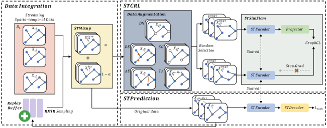
Figure 1: URCL Framework Overview

IV Methodology

We propose a framework, namely Unified Replay-based Continuous Learning (URCL), for spatio-temporal prediction on streaming data. We first give an overview of the framework and then provide specifics on each module in the framework.

IV-A Framework Overview

The framework consists of three major modules: data integration, spatio-temporal continuous representation learning (STCRL) and spatio-temporal prediction (STPrediction), as shown in Figure 1.

Data Integration. Considering that we feed data into the framework in a stream, we first sample data from the current dataset $D_{i}$ and sample historical data from a replay buffer, which stores a subset of previously learned observations, by a ranking-based maximally interfered retrieval (RMIR) sampling strategy. Then we integrate the two kinds of data with the help of the proposed spatio-temporal mixup (STMixup) mechanism, to goal being to better accumulate the spatio-temporal knowledge and alleviate catastrophic forgetting.

Spatio-Temporal Continuous Representation Learning (STCRL). In this module, a spatio-temporal SimSiam (STSimSiam) network, which is a variant of self-supervised Siamese networks [19], is adopted for holistic representation learning by means of mutual information maximization. For the assistance of self-supervised learning, we propose five different data augmentation methods, i.e., DropNodes (DN), DeleteEdges (DE), SubGraph (SG), AddEdge (AE), and TimeShifting (TS), based on the specific characteristics of spatio-temporal data. Then, the augmented data generated by two randomly selected augmentation methods are inserted into two spatio-temporal encoders (STEncoders) that share parameters with each other, followed by a projection MLP (projector).

Spatio-Temporal Prediction (STPredition). We use an STEncoder that shares the same parameters with that in STCRL to learn latent hidden features from the original data, where the learned data are then stored in the replay buffer. Finally, the learned features are input into a spatio-temporal decoder (STDecoder) for prediction.

IV-B Data Integration

To sample more representative samples from replay buffer $\mathcal{B}$, we design a novel ranking-based maximally interfered retrieval (RMIR) sampling method. Given the current data sequence $D_{i}$, we first sample M observations $\mathcal{X}_{M}=\left\langle X_{t_{i}^{k-M+1}},\cdots X_{t_{i}^{k}}\right\rangle$ starting at time slot $t_{i}^{k-M+1}$ from $D_{i}$ and select samples $\mathcal{X}_{\mathcal{B}}$ stored in the replay buffer $\mathcal{B}$, where $\mathcal{B}$ is designed to act as an explicit memory to maintain a subset of previously learned observations (i.e., the previously trained observations without STMixup). Then, the selected samples are combined with the current observations through a proposed spatio-temporal mixup (STMixup) mechanism to alleviate catastrophic forgetting by benefiting from historical observations. We can formulate the process of data integration as follows.

$$\small\centering\begin{split}\mathcal{X}_{\mathcal{B}}&=RMIR(\mathcal{B},size=|\mathcal{S}|)\\ \mathcal{X}_{mix}&=STMixup(\mathcal{X}_{M},\mathcal{X}_{\mathcal{B}}),\end{split}\@add@centering$$ (2)

where $|\mathcal{S}|$ is the sampling size.

We proceed to elaborate the RMIR sampling method and the STMixup mechanism.

IV-B1 RMIR Sampling Method

We design an RMIR sampling method to select $|\mathcal{S}|$ representative observations $\mathcal{X}_{\mathcal{B}}$ from the replay buffer. Typically, most methods in existing replay-based continuous learning methods randomly select observations from the replay memory, which leads to unsatisfied results about accuracy, due to the fact that they may ignore representative observations for replay. To select more representative samples, we first retrieve $|\mathcal{N}|$ observations $\mathcal{X}_{\mathcal{N}}$ which will be the most negatively impacted that suffer from an increase in loss by the update of foreseen parameters, where $|\mathcal{N}|\textgreater|\mathcal{S}|$. Specifically, given observation $X_{t_{i}^{\mathcal{B}}}$ in $\mathcal{B}$ and a standard objective function $\mathop{min}\limits_{\theta}\mathcal{L}_{RMIR}(f_{\theta}(X_{t_{i}^{\mathcal{B}}}),Y_{t_{i}^{\mathcal{B}}})$, where $f_{\theta}(\cdot)$ represents the URCL model, we update the parameters $\theta$ from $X_{t_{i}^{\mathcal{B}}}$ by gradient descent, as shown in Equation 3.

$$\centering\theta^{v}=\theta-\alpha\bigtriangledown\mathcal{L}_{RMIR}(f_{\theta}(X_{t_{i}^{\mathcal{B}}}),Y_{t_{i}^{\mathcal{B}}}),\@add@centering$$ (3)

where $\mathcal{L}_{RMIR}$ denotes sampling loss, $f_{\theta}(\cdot)$ represents the model, and $Y_{t_{i}^{\mathcal{B}}}$ is the ground truth. Note that Mean Absolute Error (MAE) is adopted as sampling loss. We select the top-$\mathcal{N}$ values.

Considering temporal correlations (e.g., trend and periodicity) of spatio-temporal data, data from a long time ago (periodic data) have a significant impact on the current prediction due to similarities. We then calculate the similarities between observations in $\mathcal{X}_{\mathcal{N}}$ and $\mathcal{X}_{M}$ by Pearson coefficient. Finally, we sample top-$\mathcal{S}$ observations of $\mathcal{X}_{\mathcal{N}}$ that are most similar to $\mathcal{X}_{M}$. In this way, we can not only select samples that can alleviate catastrophic forgetting, but also select samples to enhance temporal dependency capturing.

IV-B2 STMixup Mechanism

To benefit from historical observations, we introduce STMixup mechanism to fuse current observations $\mathcal{X}_{M}$ and observations $\mathcal{X}_{\mathcal{B}}$ sampled in $\mathcal{B}$. In particular, STMixup interpolates between $\mathcal{X}_{M}$ and $\mathcal{X}_{\mathcal{B}}$ to encourage the model to behave linearly across streaming spatio-temporal data sequences to minimize catastrophic forgetting.

Typically, assuming that $(x_{i},y_{i})$ and $(x_{j},y_{j})$ are two randomly selected feature-target pairs in the training data, STMixup generates virtual training examples by interpolation based on the principle of Vicinal Risk Minimization [47] to enlarge the support of the training distribution that overcomes concept drift. In STMixup, we use observation-groundtruth pairs to represent feature-target pairs in training. We use $(\tilde{x},\tilde{y})$ to denote the interpolated feature-target pair in the vicinity of the raw two pairs.

$$\small\begin{split}\tilde{x}=\lambda\cdot x_{i}+(1-\lambda)\cdot x_{j}\\ \tilde{y}=\lambda\cdot y_{i}+(1-\lambda)\cdot y_{j},\end{split}$$ (4)

where $\lambda\sim Beta(\alpha,\alpha)$, and $\alpha\in(0,\infty)$. We design STMixup by interpolating between current observations $\mathcal{X}_{M}$ and observations $\mathcal{X}_{\mathcal{B}}$ sampled from the replay buffer $\mathcal{B}$ by RMIR sampling. The interpolated observations $\mathcal{X}_{mix}$ after STMixup are formulated as follows:

$$\small\mathcal{X}_{mix}=\lambda\cdot\mathcal{X}_{M}+(1-\lambda)\cdot\mathcal{X}_{\mathcal{B}}$$ (5)

The interpolated observations $\mathcal{X}_{mix}$ can enhance a model’s ability to learn continuously by revisiting past instances in the replay buffer $\mathcal{B}$, that would be most negatively impacted by foreseen parameters. Moreover, STMixup can introduce an approximation of a regularized loss minimization [48] to avoid overfitting.

IV-C Spatio-temporal Continuous Representation Learning

The interpolated observations $\mathcal{X}_{mix}$ are input into the spatio-temporal continuous representation learning (STCRL) module for holistic feature learning. STCRL is a carefully designed self-supervised learning module, which consists of two parts: spatio-temporal data augmentation and an STSimsiam network. To enable effective spatio-temporal learning, we propose five customized spatio-temporal data augmentation methods by considering unique properties of spatio-temporal data, which transform a sample (i.e., observations in a sensor network) $\mathcal{G}=[\mathcal{X}_{mix};G]$ to its corresponding perturbation $\mathcal{G}^{\prime}$. We randomly select two different perturbations $\mathcal{G}_{1}^{\prime}$ and $\mathcal{G}_{2}^{\prime}$, and then input them into an STSimSiam network, which consists of two STEncoders $f_{\theta_{STE}}$ and a projection MLP head $h(\cdot)$. The aim of STSimSiam is to better capture spatio-temporal dependencies. Finally, STSimSiam maximizes the mutual infomation between the representations of two selected perturbations to ensure holistic feature preservation.

We proceed to elaborate the spatio-temporal data augmentation and the STSimSiam network.

IV-C1 Spatio-Temporal Data Augmentation

We augment the interpolated observations $\mathcal{X}_{mix}$ using five carefully designed spatio-temporal augmentation methods, which builds semantically similar pairs and improves the quality of the learned representations by defeating perturbations. Although existing studies propose several data augmentation methods on graph data [49, 50, 51], they do not work well for spatio-temporal data due to complex spatial and temporal correlations, especially temporal correlations (e.g., closeness). Thus, we propose five spatially oriented data augmentation methods (i.e., DropNodes (DN), DropEdge (DE), SubGraph (SG), and AddEdge (AE)) and a temporally oriented method (i.e., TimeShifting (TS)). We cover each method next.

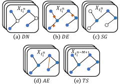
Figure 2: Spatio-temporal Data Augmentation

• DN. As shown in Figure 2(a), given a sample $\mathcal{G}=[\mathcal{X}_{mix};G]$, DN randomly discards a certain proportion (e.g., 10%) of the nodes in $G$ to get $\mathcal{G}^{\prime}=[\mathcal{X}_{mix};G^{\prime}]$ following a definite distribution (e.g., a uniform distribution), which ensures that the missing nodes have no impact on the semantics (e.g., distribution) of $G$. In particular, we mask the entries in adjacency matrix $A$ of that correspond to the discarded nodes to pertube the graph structure.

  $$\small A_{i,j}^{\prime}=\left\{\begin{array}[]{cl}0,&\mathrm{if}\,v_{i}\,\mathrm{is\,discarded}\\ A_{i,j},&\mathrm{otherwise},\end{array}\right.$$ (6)

  where $A_{i,j}^{\prime}$ is an entry of the augmented matrix $A^{\prime}$. Ideally, DN can promote model robustness by being less affected by missing data caused, e.g., sensor or communication failures.

• DE. DE randomly drops a part of edges, as shown in Figure 2(b). As the weights of sensor network $G$ are important to describe the spatial correlations between nodes (e.g., distance and similarity). We first sample a certain ratio of edges $\mathcal{E}$ from $G$ following a specific distribution, and then set a threshold $\theta_{DE}$. If the weights of edges in $\mathcal{E}$ are lower than $\theta_{DE}$, we delete the corresponding edges, formulated as follows.

  $$\centering\small a_{i,j}^{{}^{\prime}}=\left\{\begin{array}[]{cl}0,&\mathrm{if\,a_{i,j}\,<\,\theta_{DE}}\\ a_{i,j},&\mathrm{otherwise},\end{array}\right.\@add@centering$$ (7)

  where $a_{i,j}$ denotes the weight of the edge between nodes $v_{i}$ and $v_{j}$, and $a_{i,j}^{\prime}$ is the updated weight. The aim of the threshold is to retain important connectives of edges.

• SG. SG samples a subgraph $G^{\prime}=(V^{\prime},E^{\prime})$ from $G=(V,E)$ by random walk to maximally preserve the semantics of a sensor network (cf. Figure 2(c)), where $V^{\prime}\subseteq V$ and $E^{\prime}\subseteq E$. Through SG, we aim at improving local spatial correlations capturing by feature learning on the subgraph.

• AE. AE randomly selects a certain ratio of distant node pairs (e.g., more than three hops) and add edges between each node pair, which is shown in Figure 2(d). The weights of these added edges are set as the dot product similarities of corresponding node pairs. Considering a node pair $(v_{i},v_{j})$, the corresponding weight $w_{i,j}$ is calculated as follows.

  $$\small\begin{split}w_{i,j}=\vec{\mathcal{X}}^{i}_{mix}\cdot\vec{\mathcal{X}}^{j}_{mix},\end{split}$$ (8)

  where $\vec{\mathcal{X}}^{i}_{mix}$ is a vector that represents features of node $v_{i}$. The aim of AE is to strengthen the power of our model to capture global spatial correlations by connecting distant node pairs that are similar to each other.

• TS. As shown in Figure 2(e), TS, including time slicing, time warping, and time flipping, transforms current observations $\mathcal{X}_{mix}$ in $\mathcal{G}$ in the time domain. Note that we randomly select one of TS for model training.

  1. Time Slicing. Time slicing sub-samples the current observations $\mathcal{X}_{mix}$ in the time domain by randomly extracting continuous slice $\mathcal{X}_{mix}^{slice}$ with length $l$. Formally,

     $$\small\begin{split}\mathcal{X}_{mix}^{slice}=\left\langle X_{mix,t_{i}^{s-l+1}},\cdots,X_{mix,t_{i}^{s}}\right\rangle,\end{split}$$ (9)

     where $t_{i}^{k-M+1}\leq t_{i}^{s-l+1}\leq t_{i}^{s}\leq t_{i}^{k}$, $t_{i}^{k}$ is current time slot, $M$ is the length of observations, and $X_{mix,t_{i}^{s}}$ denotes observations after STMixup at time slot $t_{i}^{s}$

  2. Time Warping. Time warping upsamples sliced observations $\mathcal{X}_{mix}^{slice}$ by linear interpolation to generate warped observations $\mathcal{X}_{mix}^{warp}$, the length of it is equal to that of $\mathcal{X}_{mix}$.

     $$\small\begin{split}\mathcal{X}_{mix}^{warp}=\left\langle X^{\prime}_{mix,t_{i}^{k-M+1}},\cdots,X^{\prime}_{mix,t_{i}^{k}}\right\rangle,\end{split}$$ (10)

     where $X^{\prime}_{mix,t_{i}^{k}}$ represents the generated observations at time slot $t_{i}^{k}$.

  3. Time Flipping. Time flipping $\mathit{TF(\cdot)}$ flips the sign of warped observations $\mathcal{X}_{mix}^{warp}$ to generate a new sequence $\mathcal{X}_{mix}^{flip}$ in time domain as follows.

     $$\small\begin{split}\mathcal{X}_{mix}^{flip}=\left\langle X^{\prime}_{mix,t_{i}^{k}},\cdots,X^{\prime}_{mix,t_{i}^{k-M+1}}\right\rangle,\end{split}$$ (11)

We randomly apply two different data augmentation methods to the integrated observations $\mathcal{X}_{mix}$ (generated by STMixup) to obtain two augmented observations $\mathcal{X}_{mix}^{aug1}$ and $\mathcal{X}_{mix}^{aug2}$.

IV-C2 STSimSiam Network

Inspired by exciting feature learning ability of self-supervised learning, we design a novel STSimSiam network under the guidance of self-supervised learning to capture holistic spatio-temporal representations, inputting two randomly augmented observations $\mathcal{X}_{mix}^{aug1}$ and $\mathcal{X}_{mix}^{aug2}$. More specifically, STSimSiam consists of two STEncoders to learn spatio-temporal representations of $\mathcal{X}_{mix}^{aug1}$ and $\mathcal{X}_{mix}^{aug2}$, respectively, and a projection head to project latent embeddings of $\mathcal{X}_{mix}^{aug1}$ into the latent space of $\mathcal{X}_{mix}^{aug2}$. Finally, considering that mutual information maximization is proven to learn holistic features and thus improves continuous learning [18], we maximize the mutual information between the representations learned from $\mathcal{X}_{mix}^{aug1}$ and $\mathcal{X}_{mix}^{aug2}$ by GraphCL loss.

As shown in the upper-right corner of Figure 1, we input two randomly augmented observations $\mathcal{X}_{mix}^{aug1}$ and $\mathcal{X}_{mix}^{aug2}$ into the STSimSiam network. We first encode the two augmented observations as two fixed vectors $z_{1}$ and $z_{2}$ by STEncoders $f_{\theta_{E}}$ which are made of a specific spatio-temporal network, i.e., GraphWaveNet in this work, to capture the complex spatio-temporal dependencies. Next, we feed $z_{1}$ into a projection MLP head to map it into the latent space of $z_{2}$, which contains several MLP layers denoted as $h(\cdot)$. The process can be formulated as follows.

$$z_{1}=f_{\theta_{E}}(\mathcal{X}_{mix}^{aug1}),\quad p_{1}=h(z_{1}),\quad z_{2}=f_{\theta_{E}}(\mathcal{X}_{mix}^{aug2})$$ (12)

We use stopgrad operation $SG(\cdot)$ [52] to prevent the trivial solution obtained by STSimSiam. For example, $SG(z_{2})$ denotes that the STEncoder on $\mathcal{X}_{mix}^{aug2}$ receives no gradient from $z_{2}$.

To enhance holistic feature preservation, we employ mutual information maximization to maximize the similarities between representations of $\mathcal{X}_{mix}^{aug1}$ and $\mathcal{X}_{mix}^{aug2}$. First, for the current two augmented observations, we use cosine similarity to measure similarities $\mathcal{C(\cdot)}$ between their output vectors $p_{1}$ and $z_{2}$, formulated as follows.

$$\small\begin{split}\mathcal{C}(p_{1},z_{2})&=\frac{p_{1}}{||p_{1}||_{2}}\cdot\frac{SG(z_{2})}{||SG(z_{2})||_{2}}\\ &=\frac{h(f_{\theta}\mathcal{X}_{mix}^{aug1})}{||h(f_{\theta}(\mathcal{X}_{mix}^{aug1})||_{2}}\cdot\frac{SG(f_{\theta}(\mathcal{X}_{mix}^{aug2}))}{||SG(f_{\theta}(\mathcal{X}_{mix}^{aug2}))||_{2}},\end{split}$$ (13)

where $||\cdot||_{2}$ is $l_{2}$-$norm$.

We let $(\mathcal{X}_{mix}^{aug1},\mathcal{X}_{mix}^{aug2})$ denote an augmented observation pair. For a minibatch of $\mathcal{S}$ augmented observation pairs, we adopt a GraphCL [49] loss to maximize their mutual information. The GraphCL loss $L_{ssl}^{s}$ for the $s$-$th$ augmented observation pair is defined as follows.

$$\small\begin{split}L_{ssl}^{s}=-log\frac{exp(\mathcal{C}(p_{s,1},z_{s,2})/\tau)}{\sum_{s^{\prime}=1,s^{\prime}\neq s}^{\mathcal{S}}exp(\mathcal{C}(p_{s,1},z_{s^{\prime},2})/\tau)},\end{split}$$ (14)

where $p_{s,1}$ and $z_{s,2}$ denotes the output vectors of the $s$-$th$ augmented observation pair $(\mathcal{X}_{mix,s}^{aug1},\mathcal{X}_{mix,s}^{aug2})$, $\mathcal{C}(\cdot)$ is cosine similarity, and $\tau$ is the temperature parameter. To extract more effective features [19], we define a symmetric similarity function and obtain final $L_{ssl}^{s}$.

$$\small L_{ssl}^{s}=-log\frac{exp((\frac{1}{2}\mathcal{C}(p_{s,1},z_{s,2})+\frac{1}{2}\mathcal{C}(p_{s,2},z_{s,1}))/\tau)}{\sum_{s^{\prime}=1,s^{\prime}\neq s}^{\mathcal{S}}exp((\frac{1}{2}\mathcal{C}((p_{s,1},z_{s^{\prime},2})+\frac{1}{2}\mathcal{C}(p_{s,2},z_{s^{\prime},1}))/\tau)},$$ (15)

where $p_{s,2}=h(f_{\theta_{E}}(\mathcal{X}_{mix,s}^{aug2}))$ and $z_{s,1}=f_{\theta_{E}}(\mathcal{X}_{mix,s}^{aug1})$.

The final GraphCL loss is computed across all augmented pairs in the minibatch as follows.

$$\small L_{ssl}=\frac{1}{\mathcal{S}}\sum_{s=1}^{\mathcal{S}}L_{ssl}^{s}$$ (16)

where $\mathcal{S}$ is the batch size.

IV-D Spatio-Temporal Prediction

We design a spatio-temporal prediction network including a spatio-temporal encoder (STEncoder) and a spatio-temporal decoder (STDecoder). In particular, we input the interpolated observations $\mathcal{X}_{mix}$ into STEncoder $f_{\theta_{E}}(\cdot)$ to learn high-dimensional representations through capturing complex spatio-temporal dependencies. The STEncoder shares parameters with the STEncoder in STSimSiam. The learned representations are input into STDecoder $f_{\theta_{D}}$ for prediction. Meanwhile, the recently learned data are stored in the replay buffer. The process can be formulated as follows.

$$\small h_{\theta}=f_{\theta_{E}}(\mathcal{X}_{mix}),\quad\hat{\mathcal{Y}}=f_{\theta_{D}}(h_{\theta}),$$ (17)

where $\hat{\mathcal{Y}}$ is the prediction.

One of the advantages of our framework is its generality. It can easily serve as a plug-in for most existing spatio-temporal prediction models that follow the autoencoder architecture. GraphWaveNet [9] is one of the state-of-the-art spatio-temporal prediction models to capture precise spatial dependencies and long-term temporal dependencies, but which is not developed under the autoencoder architecture. Inspired by its excellent performance on deep spatio-temporal graph modeling, we take it as an example of spatio-temporal prediction models in our work to show how to reorganize its architecture so as to conform to the autoencoder architecture (i.e., STEncoder and STDecoder). Specifically, in STEncoder, graph convolution layers integrated with gated temporal convolution layers are employed to capture spatio-temporal dependencies, as shown in Figure 3, while several feed-forward networks are applied to map high-dimensional features into low-dimensional outputs for prediction in STDecoder, which is shown in Figure 4. It is particularly noticeable that we study the effect of different spatio-temporal prediction models (including RNN-based DCRNN [4] and attention-based GeoMAN [53]) in our experimental part in Section 5.2.4. The studies show that our framework can adapt to different prediction models. For existing spatio-temporal prediction networks that lack an STDecoder, we employ stacked MLPs as the STDecoder.

IV-D1 STEncoder

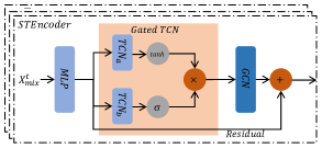
Figure 3: Illustation of STEncoder

The architecture of STEncoder is shown in Figure 3. Taking $\mathcal{X}_{mix}$ as input, an MLP layer maps it into a high-dimensional latent space, and the learned features are then input into a Gated Temporal Convolution Network (TCN) layer to learn temporal correlations among observations of the input. Next, a Graph Convolutional Network (GCN) layer is used to capture spatial correlations among the observations, where a residual operation is used to ensure accuracy. The learned features of the $i$-$th$ spatio-temporal layer can be formulated as follows.

$$\small\begin{split}h_{\mathcal{\theta}}^{i}&=f_{\mathcal{G}}(\mathit{GatedTCN}(W_{\theta}^{i}\cdot h_{\theta}^{i-1}+b^{i}_{\theta}),A),\end{split}$$ (18)

where $f_{\mathcal{G}}(\cdot)$ denotes GCN, $A$ is the adjacency matrix, $W_{\theta}^{i}$ is a learnable parameter, $b_{\theta}^{i}$ denotes the bias, and $h_{\theta}^{0}$ is euqal to $\mathcal{X}_{mix}$. The Gated TCN layer is composed of two parallel TCN layers (i.e., $\mathit{TCN_{a}}$ and $\mathit{TCN_{b}}$).

Graph Convolution Layer. Recent studies pay considerable attention to generalize convolution networks for graph data. In this work, we use spectral convolutions on the constructed sensor network, which can be simply formulated as follows:

$$\small f_{\mathcal{G}}(X,A)=\sigma(\widetilde{A}XW^{t}),$$ (19)

where $f_{\mathcal{G}}$ represents the GCN operation, $X$ denotes the node features, $\widetilde{A}=A+I_{N}$ is the adjacency matrix of $\mathcal{G}$ with added self-connections after normalizing, $W^{t}$ denotes the learnable weight matrix, and $\sigma(\cdot)$ is the activation function.

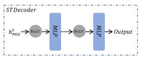
Figure 4: Illustation of STDecoder

Based on the first law of Geography: ”Near things are more related than distant things” [1], we first construct a local spatial graph by considering the geographical distance between nodes. If two nodes $v_{i}$ and $v_{j}$ are connected with each other geographically, an edge between them exists, and the corresponding weight is set as follows:

$$\small A_{i,j}=\left\{\begin{array}[]{cl}\frac{1}{dis},&\text{if $v_{i}$ connects to $v_{j}$}\\ 0,&\text{otherwise},\end{array}\right.$$ (20)

where $dis$ denotes the geographical distance between two nodes $v_{i}$ and $v_{j}$. Following Diffusion Convolutional Recurrent Neural Network (DCRNN) [4] that adopts diffusion GCN, we generalize the diffusion convolution layer into the form of Equation 19 by modeling the diffusion process of graph signals with $K$ finite steps, shown in Equation 21.

$$\small f_{\mathcal{G}}(X,A)=\sigma(\sum_{k=0}^{K}P_{k}XW_{k}),$$ (21)

where $P_{k}$ denotes the power series of the transition matrix. For an undirected graph, we can get $P=\widetilde{A}/rowsum(\widetilde{A})$, while for a directed graph, there are two directions of the diffusion process: forward direction $P^{f}=\widetilde{A}/rowsum(\widetilde{A})$ and backward direction $P^{b}=\widetilde{A}^{T}/rowsum(\widetilde{A}^{T})$. The diffusion graph convolution layer for a directed graph is derived as:

$$\small f_{\mathcal{G}}(X,A)=\sigma(\sum_{k=0}^{K}P_{k}^{f}XW_{k_{1}}+P_{k}^{b}XW_{k_{2}}),$$ (22)

However, the first law of geography may not fully reflect the spatial correlation in urban areas, especially global spatial correlations (e.g., POI similarity) [6, 2]. To tackle this problem, we construct a self-adaptive adjacency matrix $\widetilde{A}_{adp}$ by multiplying two randomly initialized node embeddings with learnable parameters $E_{1}$ and $E_{2}$:

$$\small\widetilde{A}^{adp}=\mathit{Softmax}(ReLU(E_{1}E_{2}^{T})),$$ (23)

where $\mathit{Softmax}$ is used to normalize the self-adaptive adjacency matrix. By comprehensively considering local and global spatial correlations, the final graph convolution layer is given in Equation 24.

$$\small f_{\mathcal{G}}(X,A)=\sigma(\sum_{k=0}^{K}P_{k}^{f}XW_{k_{1}}+P_{k}^{b}XW_{k_{2}}+\widetilde{A}_{k}^{adp}XW_{k_{3}}),$$ (24)

If the sensor network is unknown, we adopt the self-adaptive adjacency matrix alone to capture the spatial dependencies.

Gated Convolution Layer. To capture temporal dependencies, we employ the dilated causal convolution [54] as our TCN due to its ability of modeling long-term temporal correlations and parallel computation. Specifically, given a data sequence $\mathcal{X}$ and a filter $f$, the dilated causal convolution operation of $x$ at $j$-th step is represented as:

$$\small\mathcal{X}\circ f(j)=\sum_{m=0}^{K-1}f(m)\mathcal{X}(j-d\times m),$$ (25)

where $d$ denotes the dilation factor that reflects skipping steps, and $K$ is the length of filter $f$.

Gating mechanism is proven to be useful to control information flow through layers for TCN [55]. We adopt a simple form of Gated TCN in our work to model complex temporal correlations, where the Gated TCN only consists of an output gate. Given the observations $\mathcal{X}$, the Gated TCN is illustrated in Equation 26.

$$\small h=g(W_{1}\times\mathcal{X}+b)\odot\sigma(W_{2}\times\mathcal{X}+c),$$ (26)

where $h$ is the learned features of input modeled by the first MLP layer, $W_{1}$ and $W_{2}$ are the learnable parameters, and $b,c$ are the bias, $\odot$ denotes the element-wise product, $g(\cdot)$ and $\sigma(\cdot)$ represent activation functions (e.g., tanh and sigmod).

Algorithm 1 The URCL Framework

1:Historical streaming spatio-temporal data sequences $\mathbb{D}$ from $D_{1}$ to $D_{m}$ and a sensor network $G$

2:$i$-$th$ URCL model $\theta_{i}$

3:for $D_{i}$ in $\mathbb{D}$ do

4:     $D_{i}^{train},D_{i}^{val},D_{i}^{test}\longrightarrow\emptyset$

5:     put training, validating and testing instances into $D_{i}^{train},D_{i}^{val}$ and $D_{i}^{test}$, respectively

6:     while $not$ $converge$ do

7:         Sequentially select a batch of observations $D_{i}^{batch}$ from $D_{i}^{train}$

8:         Sample previous observations $\mathcal{X}_{\mathcal{B}}$ from the replay buffer $\mathcal{B}$

9:         $\mathcal{X}_{mix}\longleftarrow$ data fusion with STMixup by Equation 2

10:         $\mathcal{X}_{mix}^{aug1},\mathcal{X}_{mix}^{aug2}\longleftarrow$ spatio-temporal data augmentation by $DN,DE,SG,AE$ and $TS$

11:         $h_{\theta}\longleftarrow$ holistic feature learning by $STEncoder(\cdot)$ and GraphCL loss (i.e., Equation 15)

12:         $\hat{\mathcal{Y}}\longleftarrow$ prediction with $STDecoder(\cdot)$ by Equation 27

13:         Update $\theta_{i}$ based on Equation 29

14:     end while

15:     Return the learned $i$-$th$ learned model $\theta_{i}$

16:end for

IV-D2 STDecoder

The learned features are then input into the STDecoder to decode the data representations for prediction. As shown in Figure 4, the STDecoder contains several stacked feed-forward layers (i.e., MLPs) followed by activation functions (i.e., ReLU) to learn a projection function for future prediction. It can be formulated as follows.

$$\small\begin{split}\hat{\mathcal{Y}}=W_{\theta_{D}}(\alpha(h_{\theta})+b_{\theta_{D}})),\end{split}$$ (27)

where $\hat{\mathcal{Y}}$ denotes the prediction, $W_{\theta_{D}}$ is a learnable parameter, $\alpha(\cdot)$ is the ReLU activiation function, and $b_{\theta_{D}}$ is the bias.

IV-E Overall Objective Function

The overall objective of URCL is to minimize the prediction error by Mean Absolute Error (MAE) for each data stream $D_{i}$. The objective function is given in the following:

$$\small L_{task}=\frac{1}{\mathcal{L}}\sum_{l=1}^{\mathcal{L}}|\hat{\mathcal{Y}^{l}}-\mathcal{Y}^{l}|,$$ (28)

where $\mathcal{L}$ is the training sample size, $\hat{\mathcal{Y}^{l}}$ is the prediction, and $\mathcal{Y}^{l}$ is the ground truth.

The final loss contains two parts: a prediction loss of the prediction task $L_{task}$ and a GraphCL loss $L_{ssl}$ for holistic feature learning. We combine them together and the overall loss is as follows.

$$\small L_{all}=L_{task}+L_{ssl}$$ (29)

The whole process of the URCL is shown in Algorithm 1, where lines 4–5 state the data preprocessing and lines 6–14 show the training process of URCL.

V Experimental Evaluation

TABLE I: Statistics of Datasets

Dataset	METR-LA	PEMS-BAY	PEMS04	PEMS08
Area	Los Angeles	California	San Francisco Bay	San Bernaridino
Time span	4 months	5 months	2 months	2 months
Sampling interval	15 mins	15 mins	5 mins	5 mins
No. of Nodes	207	325	307	170
Input steps	12	12	12	12
Output steps	1	1	1	1

TABLE II: Performance of Training on Streaming Data on Two Datasets

Method	PEMS-BAY										PEMS08
	MAE					RMSE					MAE					RMSE
	$\mathcal{B}_{set}$	$\mathcal{I}_{set}^{1}$	$\mathcal{I}_{set}^{2}$	$\mathcal{I}_{set}^{3}$	$\mathcal{I}_{set}^{4}$	$\mathcal{B}_{set}$	$\mathcal{I}_{set}^{1}$	$\mathcal{I}_{set}^{2}$	$\mathcal{I}_{set}^{3}$	$\mathcal{I}_{set}^{4}$	$\mathcal{B}_{set}$	$\mathcal{I}_{set}^{1}$	$\mathcal{I}_{set}^{2}$	$\mathcal{I}_{set}^{3}$	$\mathcal{I}_{set}^{4}$	$\mathcal{B}_{set}$	$\mathcal{I}_{set}^{1}$	$\mathcal{I}_{set}^{2}$	$\mathcal{I}_{set}^{3}$	$\mathcal{I}_{set}^{4}$
OneFitAll	1.21	2.76	2.72	3.75	3.63	2.17	5.82	4.88	7.28	6.86	18.15	38.75	39.32	44.22	27.21	26.28	44.29	57.34	63.01	37.19
FinetuneST	1.21	3.57	3.57	3.48	3.52	2.16	7.68	7.59	7.66	7.58	18.17	32.60	33.75	34.13	33.15	26.99	37.63	39.79	33.29	35.67
URCL	1.12	1.09	1.21	1.19	1.15	1.91	1.86	2.08	2.01	1.99	18.13	18.07	17.45	17.38	17.20	26.44	26.02	25.65	24.86	24.52

V-A Experimental Setup

V-A1 Datasets

The experiments are carried out on four widely-used graph-based urban spatio-temporal datasets: METR-LA, PEMS-BAY, PEMS04 and PEMS08, where METR-LA and PEMS-BAY are related to traffic speed prediction, and PEMS04 and PEMS08 are related to traffic flow prediction.

• METR-LA. METR-LA is collected in Los Angeles County and contains the traffic data from March to June 2012 as collected by 207 sensors.

• PEMS-BAY. PEMS-BAY is collected in the Bay Area in California and contains data from 325 sensors. The time span is from January to May in 2017.

• PEMS04. PEMS04 is collected from highways in the San Francisco Bay Area and contains 3848 detectors on 29 roads. The time span is from January to February in 2018.

• PEMS08. PEMS08 is collectd in SanBernaridino from July to August in 2016. It contains the traffic data collected from 1,979 detectors on eight road segments.

We choose traffic prediction as a representative case of spatio-temporal prediction, as traffic prediction is a popular spatio-temporal prediction tasks. Dataset statistics are provided in Table I and includes area, time span, sampling interval, number of nodes, and input and output steps.

V-A2 Evaluation Methods.

We compare URCL with the following baseline methods.

• ARIMA. The Auto-Regressive Integrated Moving Average (ARIMA) method is a classic statistic-based method for time series prediction [8].

• DCRNN. The Diffusion Convolutional Recurrent Neural Network (DCRNN) method employs graph convolution networks to capture spatial correlations and the enocoder-decoder architecture with scheduled sampling to learn temporal correlations for traffic prediction [4].

• STGCN. The Spatio-Temporal Graph Convolutional Networks (STGCN) method applies ChebNet-GCN and 1D convolution to extract spatial and temporal dependencies for traffic prediction [56].

• MTGNN. The MTGNN model utilizes a graph-based deep learning method to exploit the inherent dependency relationships among multiple time series for multivariate time series forecasting [10].

• AGCRN. The Adaptive Graph Convolutional Recurrent Network (AGCRN) model captures the fine-grained spatial and temporal correlations automatically in traffic series data for traffic prediction [12].

• STGODE. The Spatial-Temporal Graph Ordinary Differential Equation Networks (STGODE) method adopts a tensor-based graph ordinary differential equation network to capture spatio-temporal dynamics and further is integrated with the temporal dilation convolution for traffic prediction [5].

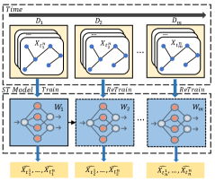
Figure 5: Illustration of Replay-based Streaming Spatio-Temporal Data Prediction

TABLE III: Overall Accuracy on Four Datasets

Dataset		Metric	ARIMA	DCRNN	STGCN	MTGNN	AGCRN	STGODE	URCL
METR-LA	$\mathcal{B}_{set}$	MAE	4.99	4.01	3.92	4.01	3.83	7.39	3.82
		RMSE	8.82	6.22	7.98	6.89	6.33	11.42	6.19
	$\mathcal{I}_{set}^{1}$	MAE	5.87	10.55	9.99	5.83	6.78	7.11	3.73
		RMSE	9.77	14.41	14.77	9.71	12.42	11.62	6.14
	$\mathcal{I}_{set}^{2}$	MAE	5.88	7.59	3.83	4.33	4.30	7.35	3.72
		RMSE	10.49	8.44	5.63	6.89	7.59	11.77	6.06
	$\mathcal{I}_{set}^{3}$	MAE	4.88	4.77	4.96	3.74	4.32	6.45	3.60
		RMSE	10.49	6.81	7.00	5.91	7.59	10.17	5.69
	$\mathcal{I}_{set}^{4}$	MAE	5.00	4.13	3.89	4.31	4.32	7.40	3.74
		RMSE	10.99	6.25	5.63	6.94	7.53	11.78	6.01
PEMS-BAY	$\mathcal{B}_{set}$	MAE	1.98	1.30	1.31	1.39	1.25	4.89	1.12
		RMSE	3.85	2.24	2.28	2.53	2.51	7.93	1.92
	$\mathcal{I}_{set}^{1}$	MAE	3.88	1.11	2.57	1.30	1.14	4.66	1.09
		RMSE	4.98	1.87	5.58	2.22	2.23	7.61	1.86
	$\mathcal{I}_{set}^{2}$	MAE	3.67	1.30	2.20	1.47	1.74	2.44	1.21
		RMSE	4.89	2.34	4.55	2.53	2.24	3.69	2.08
	$\mathcal{I}_{set}^{3}$	MAE	3.24	1.21	3.33	1.20	1.62	5.31	1.19
		RMSE	6.77	2.11	7.06	2.13	2.01	8.64	2.00
	$\mathcal{I}_{set}^{4}$	MAE	5.92	1.22	3.49	1.17	1.73	4.84	1.15
		RMSE	10.22	2.00	7.53	2.10	2.05	7.84	1.99
PEMS04	$\mathcal{B}_{set}$	MAE	56.79	24.46	31.67	22.99	22.09	36.54	19.77
		RMSE	77.89	33.85	45.33	32.99	36.32	51.70	31.26
	$\mathcal{I}_{set}^{1}$	MAE	65.78	24.34	46.29	24.76	24.65	48.55	21.56
		RMSE	87.94	39.33	62.39	35.33	40.22	67.01	34.10
	$\mathcal{I}_{set}^{2}$	MAE	67.93	23.27	59.07	29.70	21.93	49.60	21.61
		RMSE	79.02	36.68	79.47	39.64	35.97	67.40	34.04
	$\mathcal{I}_{set}^{3}$	MAE	63.92	25.95	29.08	26.04	21.34	49.99	20.97
		RMSE	75.02	35.28	33.26	35.76	32.86	68.32	32.12
	$\mathcal{I}_{set}^{4}$	MAE	62.76	23.89	23.10	25.81	20.81	49.81	20.48
		RMSE	78.22	33.42	31.14	35.79	32.66	67.69	32.20
PEMS08	$\mathcal{B}_{set}$	MAE	45.98	23.07	18.33	20.70	23.03	28.58	18.08
		RMSE	67.28	32.24	27.68	30.38	38.44	38.54	27.03
	$\mathcal{I}_{set}^{1}$	MAE	55.22	20.35	18.35	20.66	19.47	36.55	17.82
		RMSE	75.33	27.92	24.30	29.82	31.74	46.04	26.37
	$\mathcal{I}_{set}^{2}$	MAE	49.33	22.15	39.32	20.27	17.45	36.06	17.45
		RMSE	59.89	29.63	57.34	28.97	27.35	45.25	26.02
	$\mathcal{I}_{set}^{3}$	MAE	58.99	19.94	44.22	22.68	17.70	36.12	16.42
		RMSE	65.79	27.04	63.01	30.24	27.56	45.04	24.88
	$\mathcal{I}_{set}^{4}$	MAE	62.89	19.87	27.21	18.92	18.35	36.05	16.44
		RMSE	71.36	27.91	37.19	26.99	28.80	45.30	24.16

V-A3 Metrics

Mean Absolute Error (MAE) and Root Mean Square Error (RMSE) are adopted as the evaluation metrics, which are defined as follows.

$$\small\begin{split}\mathit{MAE}&=\frac{1}{M}\sum^{M}_{m=1}|\hat{\mathcal{Y}^{m}}-\mathcal{Y}^{m}|\\ \mathit{RMSE}&=\sqrt{\frac{1}{M}\sum^{M}_{m=1}||\hat{\mathcal{Y}^{m}}-\mathcal{Y}^{m}||^{2}},\end{split}$$ (30)

where $M$ is the testing data size, $\hat{y}^{t}$ is the prediction and $y^{t}$ represents the ground truth. The smaller the AME and the RMSE are, the more accurate the method is. We also evaluate the efficiency of the models, including the training and inference (i.e., testing) time.

V-A4 Other Implementation Details

We implement our model with the Pytorch framework on NVIDIA Quadro RTX 8000 GPU.

Continuous Learning Settings. We denote $D_{1}$ as a base set and $D_{2}$ to $D_{m}$ as incremental sets, where $\mathbb{D}=\left\langle D_{1},D_{2},\cdots,D_{m}\right\rangle$ ($m\geq 1$) is a sequence of streaming spatio-temporal data sequences as defined in Section III. In the experiments, we use a base set, denoted as $\mathcal{\mathcal{B}}_{set}$, and four incremental sets, denoted as $\mathcal{I}_{set}^{1}$ to $\mathcal{I}_{set}^{4}$, to facilitate continuous training. Specifically, we use $30\%$ of each dataset as the base set and the remaining data in each dataset into four equal parts to form the incremental sets. The base set and incremental sets are provided sequentially with time evolving.

Training Process. We have tried to establish fair comparisons among the baseline methods (see Section V-A2) by mapping their original training process into a continuous training processes, as shown in Figure 5. We first train an initial spatio-temporal (ST) model on base set $D_{1}$ and then re-train a new ST model on incremental sets ($D_{2}$–$D_{5}$) based on the last learned model.

Parameter Settings. The model parameters are set as follows. The input sizes for METR-LA and PEMS-BAY are $12\times 207\times 2$ and $12\times 325\times 2$, respectively, where $12$ denotes the number of the previous time slots used for prediction, $307$ and $325$ are the numbers of the nodes, and $2$ is the number of channels representing traffic speed and flow. Moreover, the input size for PEMS04 and PEMS08 are $12\times 307\times 3$ and $12\times 170\times 3$, respectively, where $3$ denotes channels representing flow, speed, and occupancy. The STEncoder in URCL contains five layers, the hidden feature dimensions of which are 32, 32, 32, 32, and 256. The STDecoder contains two layers with 512 and 12 hidden features, respectively. The output of METR-LA, PEMS-BAY, PEMS04, and PEMS08 are $1\times 207\times 1$, $1\times 325\times 1$, $1\times 307\times 1$, and $1\times 170\times 1$, respectively. We organize the buffer as a queue, whose size is set to 256. The parameters of the baseline methods are set based on their original papers and any accompanying code. Note that we normalize the streaming data into $[0,1]$ to facilitate the feature learning.

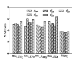
(a) MAE on METR-LA

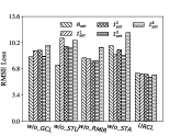
(b) RMSE on METR-LA

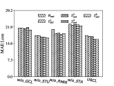
(c) MAE on PEMS08

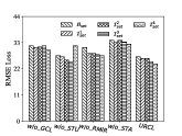
(d) RMSE on PEMS08

Figure 6: RMSE and MAE of URCL and Its Variants

V-B Experimental Results

V-B1 Performance of Training on Streaming Data

Our URCL proposes a replay-based strategy for training on streaming data, where a replay buffer is given to store previously learned samples that fuse with the training data by a spatio-temporal mixup mechanism to preserve historical knowledge effectively. To evaluate the performance of training on streaming data, two representative training strategies are used to replace the replay-based strategy in URCL and are compared with URCL: 1) OneFitAll that trains a model with the base set and then predicts all the testing data in the stream of spatio-temporal datasets; and 2) FinetuneST that trains an initial model on the base set and then fine-tunes the model with incremental sets repeatedly. GraphWaveNet is used as the base model of OneFitAll and FinetuneST. We report the MAE and RMSE results on the PEMS-BAY and the PEMS08 datasets in Table II, where the overall best performance is marked in bold. To save space, we do not report results on the METR-LA and PEMS04 datasets, as these are similar to those obtained for PEMS-BAY and the PEMS08. The results on other datasets are included in the technical report^LABEL:code.

We can see that URCL shows the best performance in terms of MAE and RMSE when compared with other methods on both datasets. More specifically, URCL outperforms the best among the baselines by $14.5\%$–$67.3\%$ and $15.5\%$–$72.4\%$ for MAE and RMSE on PEMS-BAY, respectively, and $1.2\%$–$49.1\%$ and $8.9\%$–$35.5\%$ for MAE and RMSE on PEMS08, respectively. OneFitAll and FinetuneST offer acceptable MAE and RMSE results on the base sets on both datasets, but their performance deteriorates on incremental sets. OneFitAll shows that as time goes, the new data can be different from the training data, showing that concept drift happens and a static model does not work, calling for a CL model. While a simple CL based FinetuneST is not enough, as it has forgetting problems. URCL achieves relatively stable performance on both base sets and incremental sets demonstrating its superiority.

V-B2 Overall Accuracy

We report the MAE and RMSE values of the methods in Table III. The best performance by an existing method (ARIMA, DCRNN, STGCN, MTGNN, AGCRN, and STGODE) is underlined, and the overall best performance is marked in bold. Note that we repeatably train each original baseline on each base and incremental to enable fair comparison with the replay-based strategy (like Figure 5). The observations are in the following.

• The proposed URCL achieves the best results among all baselines in most cases, performing better than the best among the baselines by up to $36.0\%$ and $34.1\%$ in terms of MAE and RMSE, respectively. In most cases, URCL outperforms the best among the baselines in terms of MAE and RMSE on the traffic speed datasets (i.e., METR-LA and PEMS-BAY) except for $\mathcal{I}_{set}^{4}$ on METR-LA. Moreover, URCL also outperforms the best among the baselines in terms of MAE and RMSE on the traffic flow datasets (i.e., PEMS04 and PEMS08) except for $\mathcal{I}_{set}^{1}$ on PEMS08. We observe that the performance improvements obtained by URCL on the traffic speed datasets exceed those on the traffic flow datasets. This is because because much more traffic flow data is available than traffic speed data. Thus, the baselines using the replay-based training strategy with sufficient data can get comparable results.

• ARIMA, a traditional statistical method, performs worse than all methods except STGODE on METR-LA and PEMS-BAY and has the worst performance among all baselines on PEMS04 and PEMS08. This is because ARIMA only uses the time-series data of each region and ignores spatial dependencies. On METR-LA and PEMS-BAY, STGODE performs the worst since it is customized for speed prediction instead of flow prediction.

• As a popular spatio-temporal prediction model, AGCRN performs the best among all the baselines in most cases, due to its powerful ability to capture spatial and temporal correlations.

From the above observations, we can see that URCL can be applied on both traffic speed and traffic flow prediction tasks, which indicates generality across prediction tasks.

V-B3 Ablation Study

To gain insight into the effects of key aspects of URCL, including the STMixup mechanism, the RMIR sampling strategy, the data augmentation methods, and the GraphCL loss, we evaluate four URCL variants:

• w/o STMixup (w/o_STU). w/o_STU is the URCL model without the STMixup module. We directly concatenate the original observations and sampled observations from the replay buffer.

• w/o RMIR Sampling (w/o_RMIR). w/o RMIR replaces the RMIR sampling mechanism from URCL with a random sampling one.

• w/o STAugmentation (w/o_STA). w/o_STA is the URCL model without the STAugmentation.

• w/o GraphCL (w/o_GCL). w/o_GCL is the URCL model without the GraphCL loss.

Figure 6 shows the MAE and RMSE results on METR-LA and PEMS08. Regardless of the datasets, URCL always outperforms its counterparts without the STMixup mechanism, the RMIR sampling strategy, the data augmentation methods, or the GraphCL loss. These four components all improve the prediction accuracy of URCL, as removing any one of them increases the MAE and RMSE values on both base sets and incremental sets. Further, on both datasets, w/o_STA performs the worst among all variants in most cases. URCL outperforms w/o_STA, reducing the MAE and RMSE values by up to $41.5\%$ and $47.8\%$, respectively, thus showing the benefit of spatio-temporal data augmentation. It is noteworthy that we include all the results in the technical report.

V-B4 Effect of Different Backbones

TABLE IV: Effect of Various Backbones on METR-LA and PEMS04

Dataset		Metric	DCRNN	GeoMAN	URCL
METR-LA	$\mathcal{B}_{set}$	MAE	4.97	5.11	3.82
		RMSE	8.18	8.47	6.19
	$\mathcal{I}_{set}^{1}$	MAE	4.76	4.87	3.73
		RMSE	8.07	8.28	6.14
	$\mathcal{I}_{set}^{2}$	MAE	4.64	4.41	3.72
		RMSE	7.80	7.09	6.06
	$\mathcal{I}_{set}^{3}$	MAE	4.61	4.39	3.60
		RMSE	7.86	7.28	5.69
	$\mathcal{I}_{set}^{4}$	MAE	5.54	5.27	3.74
		RMSE	9.59	8.77	6.01
PEMS04	$\mathcal{B}_{set}$	MAE	19.97	19.78	19.77
		RMSE	32.25	31.19	31.26
	$\mathcal{I}_{set}^{1}$	MAE	21.55	20.82	21.56
		RMSE	35.35	33.15	34.10
	$\mathcal{I}_{set}^{2}$	MAE	22.06	21.07	21.61
		RMSE	35.92	33.48	34.04
	$\mathcal{I}_{set}^{3}$	MAE	21.78	21.49	20.97
		RMSE	32.21	34.34	32.12
	$\mathcal{I}_{set}^{4}$	MAE	21.24	21.54	20.48
		RMSE	34.21	34.75	32.20

Next, we study the effect of using different backbones, which are base models. For example, the backbone of URCL is the CNN-based GraphWaveNet [10] (see Section IV-D). In addition to CNN-based models, two main streams of existing graph-based spatio-temporal prediction models exist, including RNN-based and attention-based models that adopt RNNs and the attention mechanism to learn temporal dynamics, respectively, and employ graph neural networks to capture spatial correlations. We select two representative models as the backbones of URCL, i.e., DCRNN [4] that is based on RNNs. GeoMAN [53] that is based on the attention mechanism, We then compare them with URCL. For simplicity, we use the names of the backbones as the names of the compared methods. Table IV shows the prediction results on METR-LA and PEMS04. DCRNN and GeoMAN are neck-to-neck in terms of MAE and RMSE on both datasets. URCL has the best performance in most cases, but the performance of the other two models are comparable especially on PEMS04, demonstrating the generality of URCL for adopting different backbones.

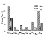
(a) Training Time

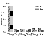
(b) Inference Time

Figure 7: Training and Inference Time on PEMS04

V-B5 Efficiency

As efficiency is important for spatio-temporal prediction on streaming data, we study the training time (of each epoch) and inference (testing) time (of each observation) for all the deep-learning-based methods on PEMS04. Figure 7 shows the training and inference time of the base sets, as well as the averages of those of all the incremental sets. One can see that the training time of URCL is lower than that of DCRNN, as shown in Figure 7(a). Although the baselines (except DCRNN) take less time for training, they perform worse than URCL in terms of prediction accuracy. Figure 7(b) shows that the inference time of URCL is far lower than that of DCRNN and is comparable with those of the other baselines, which indicates the feasibility of URCL for model deployment in real streaming spatio-temporal prediction scenarios.

V-B6 Convergence Analysis of Training

We study the training convergence of URCL on MATR-LA and PEMS08—see Figure 8. The number of epochs for training each base/incremental set is $100$, which means that we use the first $100$ epochs for training $\mathcal{B}_{set}$, the second $100$ epochs for training $\mathcal{I}^{1}_{set}$, the third $100$ epochs for training $\mathcal{I}^{2}_{set}$, and the rest can be done in the same manner. We observe that URCL converges after approximately $90$ epochs on $\mathcal{B}_{set}$ of both datasets, which shows that it converges quickly. Moreover, URCL converges after around $60$ epochs on all incremental sets of both datasets, meaning that it converges faster than on the base set. This shows that URCL can reduce the training time on the unseen data substantially and thus can reduce computational costs. In addition, the training loss curves drop smoothly, after which there are minor fluctuations on the training loss. This is mainly because the proposed STMixUp mechanism brings the benefits of regularization.

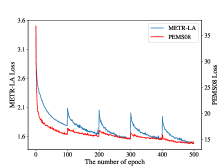
Figure 8: Training Convergence of URCL on MATR-LA and PEMS08

VI Conclusion

We propose a unified replay-based continuous learning framework for spatio-temporal prediction on streaming data, that aims to capture the complex patterns in spatio-temporal data. To embrace historical knowledge, an STMixup mechanism is designed to integrate training data with representative data sampled from a replay buffer. By coupling a spatio-temporal SimSiam network with a spatio-temporal prediction autoencoder, the holistic features are extracted through mutual information maximization. In addition, five spatio-temporal data augmentation methods are proposed to cope with the SimSiam network. An empirical study with real datasets offers evidence that the paper’s proposals improve on the state of the art in terms of prediction accuracy. An interesting research direction is to attempt to further improve the training efficiency of the proposed URCL.

VII Acknowledgment

This work is partially supported by Independent Research Fund Denmark under agreements 8022-00246B and 8048-00038B, the VILLUM FONDEN under agreements 34328 and 40567, Huawei Cloud Database Innovation Lab, and the Innovation Fund Denmark center, DIREC.

References

- [1] J. Zhang, Y. Zheng, and D. Qi, “Deep spatio-temporal residual networks for citywide crowd flows prediction,” in AAAI, 2017, pp. 1655–1661.
- [2] H. Miao, J. Shen, J. Cao, J. Xia, and S. Wang, “MBA-STNet: Bayes-enhanced discriminative multi-task learning for flow prediction,” TKDE, vol. 14, no. 8, pp. 1–14, 2022.
- [3] J. Ji, J. Wang, Z. Jiang, J. Jiang, and H. Zhang, “STDEN: Towards physics-guided neural networks for traffic flow prediction,” in AAAI, vol. 36, no. 4, 2022, pp. 4048–4056.
- [4] Y. Li, R. Yu, C. Shahabi, and Y. Liu, “Diffusion convolutional recurrent neural network: Data-driven traffic forecasting,” in ICLR, 2018, pp. 1–10.
- [5] Z. Fang, Q. Long, G. Song, and K. Xie, “Spatial-temporal graph ode networks for traffic flow forecasting,” in SIGKDD, 2021, pp. 364–373.
- [6] H. Yao, X. Tang, H. Wei, G. Zheng, and Z. Li, “Revisiting spatial-temporal similarity: A deep learning framework for traffic prediction,” in AAAI, 2019, pp. 5668–5675.
- [7] B. L. Smith and M. J. Demetsky, “Traffic flow forecasting: comparison of modeling approaches,” Journal of transportation engineering, vol. 123, no. 4, pp. 261–266, 1997.
- [8] S. Shekhar and B. M. Williams, “Adaptive seasonal time series models for forecasting short-term traffic flow,” TRR, vol. 2024, no. 1, pp. 116–125, 2007.
- [9] Z. Wu, S. Pan, G. Long, J. Jiang, and C. Zhang, “Graph wavenet for deep spatial-temporal graph modeling,” in IJCAI, 2019, pp. 1907–1913.
- [10] Z. Wu, S. Pan, G. Long, J. Jiang, X. Chang, and C. Zhang, “Connecting the dots: Multivariate time series forecasting with graph neural networks,” in SIGKDD, 2020, pp. 753–763.
- [11] R.-G. Cirstea, T. Kieu, C. Guo, B. Yang, and S. J. Pan, “EnhanceNet: Plugin neural networks for enhancing correlated time series forecasting.” in ICDE, 2021, pp. 1739–1750.
- [12] L. Bai, L. Yao, C. Li, X. Wang, and C. Wang, “Adaptive graph convolutional recurrent network for traffic forecasting,” in NeurIPS, 2020, pp. 17 804–17 815.
- [13] J. Serra, D. Suris, M. Miron, and A. Karatzoglou, “Overcoming catastrophic forgetting with hard attention to the task,” in ICML, 2018, pp. 4548–4557.
- [14] J. Hofmanninger, M. Perkonigg, J. A. Brink, O. Pianykh, C. Herold, and G. Langs, “Dynamic memory to alleviate catastrophic forgetting in continuous learning settings,” in MICCAI, 2020, pp. 359–368.
- [15] J. Kirkpatrick, R. Pascanu, N. Rabinowitz, J. Veness, G. Desjardins, A. A. Rusu, K. Milan, J. Quan, T. Ramalho, A. Grabska-Barwinska et al., “Overcoming catastrophic forgetting in neural networks,” Proceedings of the national academy of sciences, vol. 114, no. 13, pp. 3521–3526, 2017.
- [16] R. Aljundi, E. Belilovsky, T. Tuytelaars, L. Charlin, M. Caccia, M. Lin, and L. Page-Caccia, “Online continual learning with maximal interfered retrieval,” in NeurIPS, 2019, pp. 11 849–11 860.
- [17] F.-K. Sun, C.-H. Ho, and H.-Y. Lee, “Lamol: Language modeling for lifelong language learning,” ICLR, 2019.
- [18] Y. Guo, B. Liu, and D. Zhao, “Online continual learning through mutual information maximization,” in ICML, 2022, pp. 8109–8126.
- [19] X. Chen and K. He, “Exploring simple siamese representation learning,” in CVF, 2021, pp. 15 750–15 758.
- [20] J. Zbontar, L. Jing, I. Misra, Y. LeCun, and S. Deny, “Barlow twins: Self-supervised learning via redundancy reduction,” in ICML, 2021, pp. 12 310–12 320.
- [21] S. Wang, J. Cao, and S. Y. Philip, “Deep learning for spatio-temporal data mining: A survey,” TKDE, vol. 34, no. 8, pp. 3681–3700, 2020.
- [22] J. Ji, J. Wang, C. Huang, J. Wu, B. Xu, Z. Wu, J. Zhang, and Y. Zheng, “Spatio-temporal self-supervised learning for traffic flow prediction,” in AAAI, vol. 37, no. 4, 2023, pp. 4356–4364.
- [23] Z. Zhou, K. Yang, Y. Liang, B. Wang, H. Chen, and Y. Wang, “Predicting collective human mobility via countering spatiotemporal heterogeneity,” TMC, pp. 1–16, 2023.
- [24] X. Shi, Z. Chen, H. Wang, D.-Y. Yeung, W.-K. Wong, and W.-c. Woo, “Convolutional lstm network: A machine learning approach for precipitation nowcasting,” in NeurIPS, 2015, pp. 802–810.
- [25] X. Yi, J. Zhang, Z. Wang, T. Li, and Y. Zheng, “Deep distributed fusion network for air quality prediction,” in SIGKDD, 2018, pp. 965–973.
- [26] M. Lippi, M. Bertini, and P. Frasconi, “Short-term traffic flow forecasting: An experimental comparison of time-series analysis and supervised learning,” TITS, vol. 14, no. 2, pp. 871–882, 2013.
- [27] T. Kieu, B. Yang, C. Guo, R.-G. Cirstea, Y. Zhao, Y. Song, and C. S. Jensen, “Anomaly detection in time series with robust variational quasi-recurrent autoencoders,” in ICDE, 2022, pp. 1342–1354.
- [28] Y. Zhao, X. Chen, L. Deng, T. Kieu, C. Guo, B. Yang, K. Zheng, and C. S. Jensen, “Outlier detection for streaming task assignment in crowdsourcing,” in WWW, 2022, pp. 1933–1943.
- [29] T. Kieu, B. Yang, C. Guo, C. S. Jensen, Y. Zhao, F. Huang, and K. Zheng, “Robust and explainable autoencoders for time series outlier detection,” in ICDE, 2022, pp. 3038–3050.
- [30] S. Mo, Z. Bao, B. Zheng, and Z. Peng, “Towards an optimal bus frequency scheduling: When the waiting time matters,” TKDE, vol. 34, no. 9, pp. 4484–4498, 2020.
- [31] X. Chen, L. Deng, F. Huang, C. Zhang, Z. Zhang, Y. Zhao, and K. Zheng, “Daemon: Unsupervised anomaly detection and interpretation for multivariate time series,” in ICDE, 2021, pp. 2225–2230.
- [32] X. Chen, L. Deng, Y. Zhao, and K. Zheng, “Adversarial autoencoder for unsupervised time series anomaly detection and interpretation,” in WSDM, 2023, pp. 267–275.
- [33] D. Campos, M. Zhang, B. Yang, T. Kieu, C. Guo, and C. S. Jensen, “LightTS: Lightweight time series classification with adaptive ensemble distillation,” SIGMOD, vol. 1, no. 2, pp. 171:1–171:27, 2023.
- [34] X. Wu, D. Zhang, M. Zhang, C. Guo, B. Yang, and C. S. Jensen, “AutoCTS+: Joint neural architecture and hyperparameter search for correlated time series forecasting,” SIGMOD, vol. 1, no. 1, pp. 97:1–97:26, 2023.
- [35] X. Wu, D. Zhang, C. Guo, C. He, B. Yang, and C. S. Jensen, “AutoCTS: Automated correlated time series forecasting,” PVLDB, vol. 15, no. 4, pp. 971–983, 2022.
- [36] M. Li and Z. Zhu, “Spatial-temporal fusion graph neural networks for traffic flow forecasting,” in AAAI, 2021, pp. 4189–4196.
- [37] Z. Zhou, Q. Huang, K. Yang, K. Wang, X. Wang, Y. Zhang, Y. Liang, and Y. Wang, “Maintaining the status quo: Capturing invariant relations for OOD spatiotemporal learning,” in SIGKDD, 2023, pp. 3603–3614.
- [38] Y. Cheng, P. Chen, C. Guo, K. Zhao, Q. Wen, B. Yang, and C. S. Jensen, “Weakly guided adaptation for robust time series forecasting,” PVLDB, 2024.
- [39] K. Zhao, C. Guo, P. Han, M. Zhang, Y. Cheng, and B. Yang, “Multiple time series forecasting with dynamic graph modeling,” PVLDB, 2024.
- [40] Z. Chen and B. Liu, “Lifelong machine learning,” Synthesis lectures on artificial intelligence and machine learning, vol. 12, no. 3, pp. 1–207, 2018.
- [41] S. Thrun, “Is learning the n-th thing any easier than learning the first?” in NeurIPS, 1995, pp. 640–646.
- [42] P. Ruvolo and E. Eaton, “Ella: An efficient lifelong learning algorithm,” in ICML, 2013, pp. 507–515.
- [43] R. Aljundi, F. Babiloni, M. Elhoseiny, M. Rohrbach, and T. Tuytelaars, “Memory aware synapses: Learning what (not) to forget,” in ECCV, 2018, pp. 139–154.
- [44] X. Chen, J. Wang, and K. Xie, “TrafficStream: A streaming traffic flow forecasting framework based on graph neural networks and continual learning,” in IJCAI, 2021, pp. 3620–3626.
- [45] Y. Xiao, M. Liu, Z. Zhang, L. Jiang, M. Yin, and J. Wang, “Streaming traffic flow prediction based on continuous reinforcement learning,” in ICDMW, 2022, pp. 16–22.
- [46] M. Tubaishat and S. Madria, “Sensor networks: an overview,” Potentials, vol. 22, no. 2, pp. 20–23, 2003.
- [47] O. Chapelle, J. Weston, L. Bottou, and V. Vapnik, “Vicinal risk minimization,” in NeurIPS, 2000, pp. 1–7.
- [48] L. Zhang, Z. Deng, K. Kawaguchi, A. Ghorbani, and J. Zou, “How does mixup help with robustness and generalization?” ICLR, 2020.
- [49] Y. You, T. Chen, Y. Sui, T. Chen, Z. Wang, and Y. Shen, “Graph contrastive learning with augmentations,” in NeurIPS, 2020, pp. 5812–5823.
- [50] S. Thakoor, C. Tallec, M. G. Azar, M. Azabou, E. L. Dyer, R. Munos, P. Veličković, and M. Valko, “Large-scale representation learning on graphs via bootstrapping,” ICLR, 2021.
- [51] J. Zeng and P. Xie, “Contrastive self-supervised learning for graph classification,” in AAAI, 2021, pp. 10 824–10 832.
- [52] D. Madaan, J. Yoon, Y. Li, Y. Liu, and S. J. Hwang, “Representational continuity for unsupervised continual learning,” in ICLR, 2021, pp. 1–18.
- [53] Y. Liang, S. Ke, J. Zhang, X. Yi, and Y. Zheng, “GeoMAN: Multi-level attention networks for geo-sensory time series prediction,” in IJCAI, 2018, pp. 3428–3434.
- [54] F. Yu and V. Koltun, “Multi-scale context aggregation by dilated convolutions,” ICLR, 2016. [Online]. Available: http://arxiv.org/abs/1511.07122
- [55] Y. N. Dauphin, A. Fan, M. Auli, and D. Grangier, “Language modeling with gated convolutional networks,” in ICML, 2017, pp. 933–941.
- [56] B. Yu, H. Yin, and Z. Zhu, “Spatio-temporal graph convolutional networks: a deep learning framework for traffic forecasting,” in IJCAI, 2018, pp. 3634–3640.