Large Angular Momentum
Abstract
Quantum states of a spin (a qubit) are parametrized by the space , the Bloch sphere. A spin (a -state system) for generic is represented instead by a point of a larger space, . Here we study the angular momentum/spin in the limit, . The state, , where is the angular momentum operator and stands for a generic unit vector in , is found to behave as a classical angular momentum, . We discuss this phenomenon, by analysing the Stern-Gerlach experiments, the angular-momentum composition rule, and the rotation matrix. This problem arose from the consideration of a macroscopic body under an inhomogeneous magnetic field. Our observations help to explain how classical mechanics (with unique particle trajectories) emerges naturally from quantum mechanics in this context, and at the same time, make the widespread notion that large spins somehow become classical, a more precise one.
1 Introduction
It is a widely shared view that in the limit of large spin (angular momentum) the quantum-mechanical spin somehow becomes classical. After all, the large spin limit () is equivalent to the limit, and, in accordance with the general idea of the semi-classical limit, physics of large angular momentum is expected to become that of classical angular momentum. But to the best of the authors’ knowledge, it has not been clearly exhibited in the literature how exactly this works 111Understandably, there is a vast literature about large angular momentum, from the early days of quantum mechanics to today, in a wide range of research fields, in various contexts and problems, and also based on different motivations. In order to avoid being biased and necessarily incomplete, we shall refrain in this work from attempting to cite or comment on any of them.. It is the aim of this note to fill in this gap.
The question came under a sharp focus in a general discussion on emergence of classical mechanics for a macroscopic body from quantum mechanics [1, 2]. Knowing about the typical Stern-Gerlach (SG) process for a spin atom, we ask what happens if a macroscopic body consisting of many (e.g. spins is set under an inhomogeneous magnetic field of a SG set-up. In general, with many spins oriented in different directions, the problem does not arise, as the bound-state Hamiltonian does not allow each component particle to split à la SG into spatially separated sub-wavepackets. Logically, however, one cannot exclude the special situation in which a large number of spins are all oriented in the same direction. Such a large spin system might continue to behave quantum-mechanically, e.g. with a typical SG spreading of the wavepackets, even in the limit.
It will be shown that the state , the state in which the large spin is oriented in some direction , behaves instead as a classical angular momentum, yielding the unique trajectory in the SG processes (Sec. 2). This result leads us to consider more carefully in Sec. 3 the relation between the space of quantum-mechanical angular-momentum states and that of classical angular momenta, and to identify the special class of quantum angular momentum states to be put in correspondence with the classical angular momentum (see Eqs. (3.11), (3.12), (3.13) below). The content of the present work is to check the consistency of this picture, through the analysis of the SG experiments (Sec. 2), the angular-momentum composition rule (Sec. 4), and the rotation matrix (Sec. 5). We conclude with a brief reflection in Sec. 6.
2 Stern-Gerlach experiments
2.1 Spin atom
For definiteness let us take an incident atom with spin directed along a definite, but generic, direction , i.e.
| (2.1) |
| (2.2) |
When the atom passes through a region with an inhomogeneous magnetic field,
| (2.3) |
the wave packet splits into two subpackets, with respective weights, and : they manifest as the relative intensities of the image bands on the screen at the end.
The original Stern-Gerlach experiment [3] has had a fundamental impact to the development of quantum theory, in proving the quantization of the angular momentum, the existence of half-integer spin, and more generally, demonstrating the quantum-mechanical nature of the center of mass (CM) of the silver atom [2].
2.2 Large spin
A classical particle with a magnetic moment directed towards
| (2.4) |
moves in an inhomogeneous magnetic field (2.3), according to Newton’s equations,
| (2.5) |
The way the unique trajectory for a classical particle emerges from quantum mechanics has been discussed in Ref. [1], where the magnetic moment is the expectation value
| (2.6) |
taken in the internal bound-state wave function where and denote the intrinsic magnetic moment and the one due to the orbital motion of the -th constituent atom or molecule (), respectively. Clearly, in general, the considerations made in Sec. 2.1 for a spin atom, with a doubly split wavepacket, cannot be simply generalized to (or compared with) a classical body (2.6) with constituents.
Typically, the spins are oriented along different directions, but the particles carrying them are bound in the macroscopic body made of atomic, molecular and larger structures. The wave function of particles in bound states does not split in sub-wavepackets, as that of an isolated spin atom does, under an inhomogeneous magnetic field. The bound-state Hamiltonian does not allow it 222This discussion is indeed closely parallel to the question of quantum diffusion. Unlike free particles, particles in bound states (the electrons in atoms; atoms in molecules, etc.) do not diffuse, as they move in binding potentials. This is one of the elements for the emergence of the classical mechanics, with unique trajectories for macroscopic bodies. As for the center-of-mass (CM) wave function of an isolated macroscopic body, its free quantum diffusion is suppressed by mass.. What determines the motion of the CM of the body is the average magnetic moment, (2.6). Logically, nevertheless, one cannot exclude special cases (e.g. a magnetized piece of metal) of all spins of the body oriented in the same direction. One might wonder how the wave function of such a particle with spin behaves, under an inhomogeneous magnetic field.
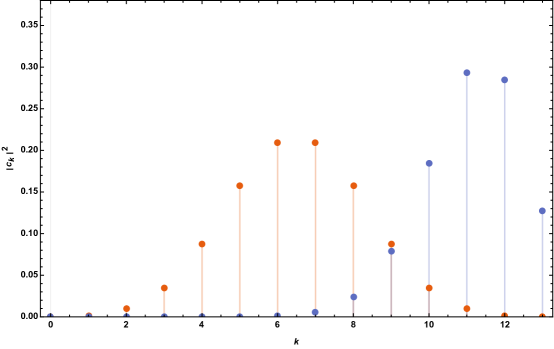
The question is whether the conditions enlisted in Ref. [1] (see Appendix A), for the emergence of classical mechanics for a macroscopic body with a unique trajectory, are sufficient, or whether some extra condition (or a new mechanism) is required, to suppress possible wide spreading of the wave function into many sub-packets (see Fig. 1 for a small spin, ) under an inhomogeneous magnetic field.
The answer turns out to be simple but somewhat unexpected. The following discussion, up to Eq. (2.15), is taken almost verbatim from Sec. 3.1.3 of Ref. [2]; for the present work it represents the starting point, and serves as the main tool of analysis below.
Consider the state of a spin directed towards a direction ,
| (2.7) |
Choosing the magnetic field (and its gradients) in the -direction, we need to express as a superposition of the eigenstates of (),
| (2.8) |
The expansion coefficients are known:
| (2.9) |
where are the binomial coefficients.
To get (2.9), let us consider (2.7) as a direct product of spin particles, (2.2),
| (2.10) |
all oriented in the same direction. Expanding and collecting terms with a fixed (the number of spin-up particles) one arrives at Eq. (2.9).
Using Stirling’s formula, one can derive, for large values of both and with fixed, the distribution across different values of ,
| (2.11) |
with
| (2.12) |
The saddle-point approximation, valid at , yields
| (2.13) |
and thus
| (2.14) |
in the ( fixed) limit. The narrow peak position corresponds to (see Eq. (2.8))
| (2.15) |
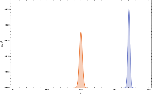
This means that a large spin () quantum particle with spin directed towards , in a Stern-Gerlach setting with an inhomogeneous magnetic field (2.3), moves along a single trajectory of a classical particle with , instead of spreading over a wide range of split sub-packet trajectories covering . See Fig. 2, cfr. Fig. 1.
This (perhaps) somewhat surprising result shows that quantum mechanics (QM) takes care of itself, so to speak, in ensuring that a large spin particle () traces a classical trajectory. This is consistent with the known general behavior of the wave function in the semi-classical limit () 333Of course this does not mean that the classical limit necessarily requires or implies , though.. Note that if the value is understood as due to the large number of spin particles composing it (see the comment after (2.9)), the spike (2.13), (2.14) can be understood as due to the accumulation of a huge number of microstates giving .
Another, equivalent way to see the shrinkage of the distribution in , (2.14), is to study its dispersion. Given the relative weights , (2.9), where and , with , it is a simple exercise to find that
| (2.16) |
so that the dispersion (the fluctuation width) is given by
| (2.17) |
It follows that
| (2.18) |
i.e. it is an infinitely narrow Gaussian. Note that the SG set-up is indeed a measurement of in the state (2.7). The fact that the result is always with no dispersion, means that it is a classical angular momentum (see Eqs. (3.11), (3.12) below).
2.2.1 Density matrix
The same phenomenon can be seen also by using the density matrix. Being the state (2.7) a pure state, its density matrix is given by
| (2.19) |
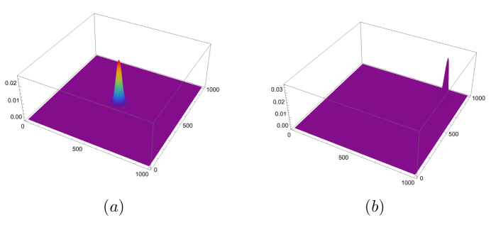
where are given in Eq. (2.9). In the limit as , it can be observed that it essentially reduces to a single diagonal element, provided that the fluctuations of the order of are neglected in comparison to . The density matrix for , with and , is depicted in Figs. 3.
2.2.2 The state preparation and successive SG set-ups
For a small , as it is well known, the SG set-up can be used to prepare any desired state , by an intentionally biased SG apparatus, e.g. in which all the split sub-wavepackets are blocked, except for the one corresponding to . Equivalently, one may use the so-called null-measurements (see Ref. [4] for a recent review). In any case, for a small finite , where there are well-separated sub-packets (see Fig. 1), there is no difficulty in extracting any desired quantum state for subsequent experiments (state preparation).
In the large-spin limit () we are considering, since there is essentially only one wavepacket present (see (2.15)), there is no possibility of extracting or selecting the desired sub-wavepacket. The experimental resolution would not allow it. We have in mind a macroscopic scenario where, in comparison to the finite region (in principle) occupied by the waves , the fluctuations of the values of around (2.15) are of the order of , i.e. of zero width.
We might consider introducing a second set of Stern-Gerlach (SG) magnetic fields directed in a different direction, denoted by , as a new quantization axis. This setup allows us to study the state emerging from the first set of SG magnetic fields (without the presence of an imaging screen),
| (2.20) |
Since the sum of states around is essentially equal to the complete sum, this state can be rewritten in terms of the eigenvalues , where correspond to the eigenvalues of as:
| (2.21) | |||||
This represents an expansion of the original state as a linear combination of the eigenstates of . In the limit , the results from Section 2.2 tell us that the sum is dominated by the small region around , with negligible fluctuations. The trajectory remains unique, regardless of the choice of quantization axis (i.e. the direction of the magnetic field) .
2.2.3 States almost directed towards
Obviously, in the large spin limit, other states close to ,
| (2.22) |
(i.e. the spin roughly oriented towards ) will behave similarly. For instance, the state is (cfr. Eq. (2.10))
| (2.23) | |||||
where and (), are two spins oriented towards , (2.8), as already studied in Sec. 2.2. In the limit, the sum is dominated by terms with . The SG projection of this state onto the eigenstates is therefore approximated by
| (2.24) |
where the results of Sec. 2.2 have been used. A similar result holds for for any finite , showing that all these states behave as a classical angular momentum, .
3 Quantum and classical angular momentum states
Before proceeding, we must discuss the correspondence between the quantum mechanical angular momentum states and their classical counterparts, more carefully. The spin (two-state system) wave function is given by
| (3.1) |
where with , describes the points of . We note that for a spin , any pure state (3.1) can be interpreted as the state in which the spin is oriented in some space direction , as in Eq. (2.2), without loss of generality. This is because the manifold of pure spin quantum states and that of the unit space vector are both . Indeed, given the state (2.2), there is always a rotation matrix such that
| (3.2) |
We recall that the general rotation matrix for a spin is given, using Euler angles 444Note that the third Euler angle (the rotation angle about the final -axis) is redundant here, as it gives only the phase , and has been set to in (3.2). (), as follows
| (3.3) |
The situation is different for a generic spin 555In this section we denote the general angular momentum (including orbital angular momentum) by , rather than , a symbol adopted commonly to indicate the spin (the intrinsic angular momentum of a particle). In this work we will use both and . Likewise, we shall use the terms “spin” and “angular momentum”, interchangeably.. The wave function now has the form,
| (3.4) |
where
| (3.5) |
are the coordinates of the space . On the other hand, the variety of the directions in the three-dimensional space, , is always . It means that the state of the spin oriented towards a definite direction (2.8), is not a general pure spin state, but belongs to a small subset, . In other words, not all states of spin , as described in (3.4), can be transformed by a rotation matrix (selecting an appropriate new axis) into the form:
| (3.6) |
These considerations highlight a potential subtlety in our argument that quantum mechanical angular momentum states somehow become classical in the large limit.
Let us recall that because of the commutation relations
| (3.7) |
only one of the components, e.g. , can be diagonalized together with the total (Casimir) angular momentum, ,
| (3.8) |
In the state, , where has a definite value, , and are fluctuating. Their magnitudes are found to be
| (3.9) |
Therefore, in a generic state , there are strong quantum fluctuations of and at . There is no way such a state can be associated with a classical angular momentum, which requires all three components to be well-defined simultaneously.
The exception occurs for states , for which
| (3.10) |
For these state, it makes sense to interpret them “classically” as angular momentum pointed towards , as its fluctuations ) become negligible with respect to its magnitude , in the limit . The same holds true in all states in which spin is oriented towards a generic direction , as has been already noted in the previous section, Eqs. (2.16)-(2.18). Accordingly, we propose the correspondence (by setting )
| (3.11) |
where
| (3.12) |
Actually, all states “almost oriented towards ”,
| (3.13) |
discussed in Sec. 2.2.3 (see (2.22)), can also be interpreted as . The aim of our present investigation is to examine the consistency of such a picture, with respect to the SG processes (this has already been done in Sec. 2.2), the addition rule of the angular momenta (Sec. 4 below) and the rotation matrix (Sec. 5 below).
As for the states with strong quantum fluctuations , (3.9) (with generic and not close to ), they are certainly quantum mechanical, independently of . The same can be said of a generic spin wave function, (3.4). If such a particle is sent into a SG set-up, it could split in an arbitrary distribution of sub wavepackets, in contrast to the cases discussed in Sec. 2.2. This results in a macroscopic quantum system. It is possible that such a strongly fluctuating, macroscopic quantum angular-momentum state can be realized experimentally, if the whole system is brought to extremely low temperatures near 666We recall that any system is in its quantum-mechanical ground state at . Accordingly many macroscopic systems can be brought to a quantum-mechanical state, if sufficiently low temperatures can be attained. See the references cited in [1] for the recent efforts to fabricate such systems experimentally..
To see what happens at finite temperatures (either the body-temperature of the macroscopic body, or a warm environment) instead, it is useful to recall the so-called Born-Einstein dispute and its resolution (see [1]). Einstein strongly rebuked the idea by Born, that the absence of quantum diffusion is sufficient to explain the classical nature (the unique trajectoriy) of a macroscopic body, arguing that a doubly or multiply split wave packet, with their centers separated by macroscopic distances, are allowed by Schrödinger equations even for a macroscopic particle. The latter is certainly non-classical. The missing piece for solving this puzzle turns out to be the temperature [1]. Even though at exceptionally low temperatures such a state is possible, it is not so at finite temperatures. Emission of photons and the ensuing self-decoherence (in the case of an isolated body) [1] or an environment-induced decoherence (for an open system) [5, 6, 7] makes a split system a mixture (a mixed state) essentially instantaneously. Also, they cannot be prepared experimentally, e.g., by a passage through a double slit [1]. A (macroscopic) particle passes either through one or the other slit, due to absence of diffusion.
A similar consideration applies to the general angular momentum states with strong fluctuations, (3.9) or (3.4). In the large limit, such a state necessarily involves large space extension: a macroscopic quantum state. A macroscopic pure quantum state can be realized only at exceedingly low temperatures 777To tie up possible loose ends of the argument, let us note that a single, spin isolated atom in its ground state (a microscopic system) travelling in a good vacuum, has effectively . Thus the fact that its split wave packets can attain a macroscopic extension - i.e. its being in a macroscopic quantum state - is perfectly consistent. To realize a macroscopic system (made of many atoms and molecules) in a pure quantum state is another story: it is much more difficult to prepare the necessary low temperatures close to . . See [1] for more discussions. At finite temperatures, macroscopically split wave packet of such a particle under the SG set-up is necessarily an incoherent mixture.
What is rather remarkable, perhaps, is the fact that the angular momentum states of minimum fluctuations, (3.12), (3.13), though pure, effectively become classical at , without need of any (thermal or environment-induced) decoherence effects, hence independently of the temperatures. This is in agreement with the known general semi-classical behavior of a (pure-state) wave function in QM in the limit .
3.1 Orbital angular momentum
All our formal arguments (3.7)–(3.13) apply equally well, both to spin (the intrinsic angular momentum of a particle or the total angular momentum of the center of mass of a body in its rest frame) and to orbital angular momentum. However, our primary tool of analysis is the Stern-Gerlach (SG) set-up (Sec. 2.2), which is more suitable for spin than for an angular momentum associated with the orbital motion of a particle. One might wonder how the large angular momentum limit works for the latter. Here is a brief acccount.
The (angular part of the) wave function of a particle in the state corresponds to the spherical harmonics,
| (3.14) |
where are the associated Legendre polynomials. Let us consider the state of minimum fluctuation, (see Eq. (3.10)). It is easy to see that the angular distribution is strongly peaked at at large ,
| (3.15) |
For instance, see Fig. 5 for . In states with stronger fluctuations ( not close to ), the distribution instead covers a large portion of the D solid angle, for any (see Fig. 5 for ).
Now a classical angular momentum has its all three components well defined. By choosing an appropriate coordinate system, it can be written as . It describes a particle moving in the plane, with . The large limit of the wave function , (3.15), describes precisely such a motion.
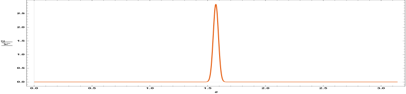
the state with .
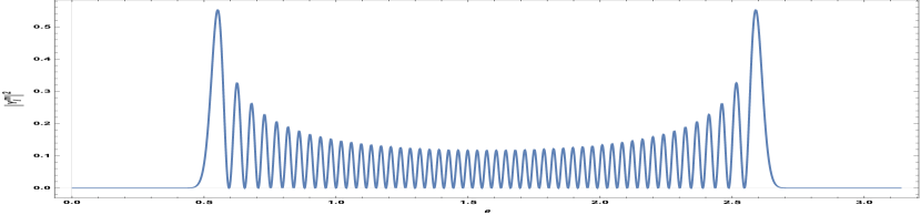
the state with , .
4 Addition of angular momenta
Let us now consider two spins, and . The composition-decomposition rules in QM is well known, i.e.
| (4.1) |
where , , indicates the multiplet (the irreducible representation) of SU(2) 888We recall that SU(2) is the simply-connected double cover of the orthogonal group SO(3)., with multiplicity and with . We set here.
We wish to find out how the addition rule looks like in the limit . For the reasons discussed in Sec. 3, we are particularly interested in the composition rule for angular momentum states with minimum fluctuations, of the form, . Therefore, let us consider two particles (spins) in the states,
| (4.2) |
namely, they are spins oriented towards the directions, and , respectively. Our aim is to find out the properties of the direct product state,
| (4.3) |
in the large limit. Since the choice of the axes is arbitrary, we may take
| (4.4) |
Then the product state is just
| (4.5) |
where is the highest state. We added the tilde sign on to indicate that it is the vector in the reference system of (4.4). Now in the limit has been studied in Sec. 2. It is
| (4.6) |
where the sum is dominated by the values of around
| (4.7) |
Since the eigenvalues of simply add up in the product state, the expansion of in the eigenstates of is dominated by terms
| (4.8) |
Exchanging and and repeating the arguments, one finds also that
| (4.9) |
But which quantum angular-momentum state does the product state (4.3) represent? The answer is that
| (4.10) |
where and the unit vector are such that (i.e. defined by)
| (4.11) |
The proof of this is as follows. By selecting the directions of the SG magnets directions (the quantization axis) to or to on the state , (4.11), one can apply the results of Sec. 2.1 to get exactly the results (4.8) or (4.9), respectively. Now, according to the quantum-classical correspondence (Eq. (3.11) and Eq. (3.12)), the state (see Eq. (4.11)) translates to
| (4.12) |
But, in view of (3.11), this is precisely the addition rule of the two classical angular momenta (i.e. a vector sum).
To be complete, one must check that the projection on any generic direction works correctly. By using the result of Sec. 2 for the SG projection on a new axis, one finds
| (4.13) |
where we made use of the fact that and commute and the eigenvalues of their components just sum up in the direct product state. Also, to be conservative, we have left unknown. However,
| (4.14) |
thus
| (4.15) |
by again using the results of Sec. 2.1 in Eq. (4.13). In conclusion, the direct product state, (4.2), (4.3), has a simple classical interpretation. It corresponds to the classical sum (the vector addition) of two angular momenta.
From the perspective of the general composition rule of two angular momentum states (4.1), what we have seen are the results concerning a specific pair of states (i.e. those of minimum fluctuations) in and , characterized by the “orientations” and . The total angular momentum magnitude in the product state (4.11) satisfies
| (4.16) |
depending on the relative orientation of and . This is consistent with the quantum-mechanical addition law, (4.1).
5 Rotation matrix
The rotation matrix for a general spin can be constructed by taking the direct products of the rotation matrix for spin , i.e. (3.3). This is based on the fact that any angular momentum state, , can be constructed as the system made of spin particles, completely symmetric under exchange of the particles, a fact already conveniently used in Sec. 2.1. The theory of angular momentum can be fully reconstructed this way [8] by using the operators,
| (5.1) |
where are the Pauli matrices, are the harmonic-oscillator annihilation and creation operators, of spin-up () and spin-down () particles,
| (5.2) |
By construction, all states , with ’s and ’s () are symmetric under exchanges of the spins, therefore belong to the irreducible representation , with 999In the SU(2) group, any irreducible representation can be constructed from the direct products of spin ’s which are totally symmetric, so no generality is lost. An anaologous construction for the SU() group, , works only for totally symmetric representations, ..
The rotation matrix for a generic spin is simply (writing the Euler angles symbolically as ) the direct productof the rotation matrices for spin , (3.3),
| (5.3) |
symmetrized () with respect to , where
| (5.4) |
It acts on the multiplet,
| (5.5) |
The action of on particular states,
| (5.6) |
where is given in Eq. (2.2), i.e. on the states with all spin ’s oriented in the same direction, is very simple. It is just the operation of rotating each and all spins towards the direction (setting ),
| (5.7) |
This corresponds precisely to the rotation of a vector,
| (5.8) |
where is the standard rotation matrix of classical mechanics.
6 Conclusion
The observations made in this note render the concept that a spin () (or angular momentum, ) becomes classical in the limit, , a more precise one. In particular, we found the identification between the states with minimum fluctuations ((3.11), (3.12), and (3.13)) with classical angular momentum vectors in such a limit, and verified its consistency through the analyses of SG experiments, of the angular-momentum addition rule, and of the rotation matrix.
At the same time, our analysis has revealed a subtlety in the quantum-classical correspondence in this context. It reflects the difference between the spaces of the quantum-mechanical and classical angular momentum states of definite magnitude ( and , respectively). It is the angular momentum states of minimum fluctuations, (3.11), (3.12), (3.13), that naturally smoothly transit into classical angular momentum in the limit, independently of temperatures. On the other hand, more general, strongly fluctuating angular momentum states belonging to are possible as pure quantum states only at exceedingly low temperatures. The reason is that in the limit such a state necessarily involves a large space extension, in a way or other. A macroscopic system is necessarily in a mixed state at finite temperatures [5, 6, 7],[1]. For instance, no macroscopically split pure wave packets in a SG setting survive decoherence effects.
The idea that a large spin is made of many spin particles seems to be a fruitful one both mathematically and physically. From the mathematics point of view, the entire theory of angular momentum can be reconstructed this way [8], as we recalled already, and it helps to recover certain formulas easily. It looks also useful from physics point of view, as such a large angular momentum system may be regarded as an idealized model of a macroscopic body, made of many atoms and molecules (spins). The sharp spike of the SG projection of the state in the narrow region around can then be understood as a results of a large number of microscopic states of atoms (spins) accumulating to give such a value of .
The various form of suppression of the fluctuations of angular momentum components we observed in this note in the limit, is in fact analogous to the “ law” invoked by Schrödinger [9], to explain the exactness (classicality) of laws of macroscopic world based on statistical mechanics, although, here, the relevant fluctuations are quantum-mechanical ones.
Acknowledgments
The work by KK is supported by the INFN special-initiative project grant GAST (Gauge and String Theories). We are grateful to Hans-Thomas Elze, Jarah Evslin, Riccardo Guida, Pietro Menotti and Arkady Vainshtein for useful comments and precious advices.
References
- [1] K. Konishi, “Newton’s equations from quantum mechanics for a macroscopic body in the vacuum”, Int. Journ. Mod. Phys. A 38 2350080 (2023).
- [2] K. Konishi and H. T. Elze, “The Quantum Ratio”, Symmetry, 16 (4) 427 (2024).
- [3] W. Gerlach and O. Stern, “Der experimentelle Nachweis der Richtungsquantelung im Magnetfeld”, Zeitschrift für Physik. 9 349-352 (1922).
- [4] K. Konishi, “On the negative-result experiments in quantum mechanics”, arXiv:2310.01955 [quant-ph]] (2023).
- [5] E. Joos and H. D. Zeh, “The emergence of classical properties through interaction with the environment”, Z. Phys. B 59, 223-243 (1985).
- [6] W. H. Zurek, “Decoherence and the Transition from Quantum to Classical”, Physics Today 44 (10), 36-44 (1991).
- [7] M. Tegmark, “Apparent wave function collapse caused by scattering”, Found. Phys. Lett. 6, 571-590 (1993).
- [8] J. Schwinger, “On Angular Momentum”, World Scientific Series in 20th Century Physics, A Quantum Legacy, 173-223 (2000). A reproduction of a book chapter from L. C. Biedenharn, H. van Dam, “Angular Momentum in Quantum Physics”, New York, Academic Press (1965).
- [9] E. Schrödinger, “What is life?”, Cambridge University Press, (1944).
Appendix A Newton’s equation for a macroscopic body
The conditions needed for the CM of an isolated macroscopic body at finite body temperatures to obey Newton’s equations have been discussed in great care by one of the present authors [1]. They are
-
(i)
For macroscopic motions (for which ) the Heisenberg relation does not limit the simultaneous determination – the initial condition – of the position and momentum;
-
(ii)
The absence of quantum diffusion, due to a large mass (a large number of atoms and molecules composing the body);
-
(iii)
A finite body temperature, implying the thermal decoherence and mixed-state nature of the body.
Under these conditions, the CM of an isolated macroscopic body has a unique trajectory. Newton’s equations for it follow from the Ehrenfest theorem. See Ref. [1] for various subtleties and for the explicit derivation of Newton’s equation under external gravitational forces, under weak, static, smoothly varying external electromagnetic fields, and under a harmonic-oscillator potential. Somewhat unexpectedly, the environment-induced decoherence [5, 6, 7] which is extremely effective in rendering macroscopic states in a finite-temperature environment a mixture, has been found not to be the most essential elements for the derivation of classical mechanics from quantum mechanics [1, 2].