Distributed Fractional Bayesian Learning for Adaptive Optimization

Abstract

This paper considers a distributed adaptive optimization problem, where all agents only have access to their local cost functions with a common unknown parameter, whereas they mean to collaboratively estimate the true parameter and find the optimal solution over a connected network. A general mathematical framework for such a problem has not been studied yet. We aim to provide valuable insights for addressing parameter uncertainty in distributed optimization problems and simultaneously find the optimal solution. Thus, we propose a novel Prediction while Optimization scheme, which utilizes distributed fractional Bayesian learning through weighted averaging on the log-beliefs to update the beliefs of unknown parameter, and distributed gradient descent for renewing the estimation of the optimal solution. Then under suitable assumptions, we prove that all agents’ beliefs and decision variables converge almost surely to the true parameter and the optimal solution under the true parameter, respectively. We further establish a sublinear convergence rate for the belief sequence. Finally, numerical experiments are implemented to corroborate the theoretical analysis.

Fractional Bayesian Learning, Distributed Gradient Descent, Consensus Protocol, Multiagent System.

1 Introduction

1.1 Backgrounds and Motivations

Distributed optimization has been widely used for modeling and resolving cooperative decision-making problems in large-scale multi-agent systems including economic dispatch, smart grids, automatic controls, and machine learning (see e.g., [1, 2]). However, in many complex situations, agents need to make decisions with uncertainty. For example, in Robotics, planning the task for a robot requires predicting other agents’ reactive behaviors which might be unknown at the very beginning [3]. In Autonomous Driving, vehicles need to interpret the intentions of others and make trajectory planning for itself[4]. In Economics of Markowitz profile problem, one should learn the uncertain parameters of expectation or covariance matrices associated with the stocks model, and then find the best solution to the optimal portfolio [5]. These together motivate us to investigate the distributed decision-making problems with model uncertainty.

Generally speaking, the resolution of decision-making problems with model uncertainty consists of two processes: model construction and decision making[6], i.e., agents need to estimate the unknown model function (the classical setting is characterized by known function structure while with unknown parameters) and find the optimal solution to it. The commonly used approaches include the sequential and simultaneous methods. However, a sequential method that considers optimization after prediction may not be applicable to complex decision-making scenarios, since large-scale parameter learning problems lead to a long time waiting for solving the original problem. Besides, as has been analyzed in [7], this scheme provides an approximate solution to model parameters, which propagates the corrupt error into the objective optimization. In some practical scenarios, optimization after prediction may lead to a “frozen robot" problem as pointed out in [8]. Therefore, developing dynamic learning coupled algorithm that consider prediction while optimization is crucial and has gained increasing popularity in recent years, see e.g., [9, 8, 7].

It is noticed that the aforementioned works [3, 4, 5, 9, 8] investigate the coupled phenomenon between model construction and decision making in specific scenarios and develop corresponding methods. However, the general mathematical framework and its resolution along with convergence analysis in large-scale distributed problems are rarely studied. The previous theoretical works in this field mostly focus on the centralized problem with parameter uncertainty, and merely consider the unidirectional coupling of optimization and prediction where the estimation of the model parameter is independent of decision making[10, 11, 12, 13]. Moreover, few of them have investigated the large-scale distributed scenarios.

We consider the bidirectional coupling of parameter learning and objective optimization, which brings more difficulties to the resolutions along with theoretical analysis. Though there exist some related works, most of them assume that the unknown parameter influences the objective function in a specific structure. For example, [14] considers a distributed quadratic optimization problem with the unknown model parameter being the objective coefficients, and adopts the recursive least square to estimate the parameter and gradient tracking to solve the objective optimization. While the work [14] imposes some assumptions on the intermediate process, which however is lack of strict theoretical verification. As a result, bidirectional coupling optimization problem has not been fully resolved here. In addition, [15] uses weighted least square to solve the unknown coefficient matrices in linear-quadratic stochastic differential games. Different from objective functions of such particular structures, we consider a more general distributed bidirectional coupling mathematical formulation and give rigorous convergence analysis.

1.2 Problem Formulation and Challenges

We characterize the uncertainty of the distributed optimization problem in a parametric sense. Our primary objective is to establish the model parameters in a way that the action generated from this estimated model best matches the observed action, meanwhile, find this best-estimated model’s optimal solution. To be specific, we consider a distributed optimization problem with unknown model parameter $\theta$ as follows.

$$\min_{x\in\mathbb{R}}~{}\frac{1}{N}\sum_{i=1}^{N}J_{i}(x,\theta_{*}),\theta_{*}\in\Theta,$$ (1)

where $J_{i}(x,\theta_{*})$ represents the private cost function of agent $i\in\mathcal{N}:=\{1,2,\cdots,N\}$. The unknown true parameter $\theta_{*}$ is taken from a finite set $\Theta:=\{\theta_{1},\theta_{2},\cdots,\theta_{M}\}$. This type of problem setting is frequently encountered in specific real-world scenarios. For example, the unknown intention of vehicles in autonomous driving can be lane-merging, maintaining driving along the right lane, and maintaining along the left lane[4], which means that the unknown parameter set is composed of three elements.

Each agent $i\in\mathcal{N}$ has a prior belief $q_{i}(\theta_{m}),m=1,2,\cdots,M$ of the $M$ possible parameters. Given an input strategy $x$, the feedback is realized randomly from a probability distribution depending on the system’s true parameter $\theta_{*}$, i.e. the noisy feedback $y_{i}=J_{i}(x,\theta_{*})+\epsilon_{i}(x,\theta_{*})$ for every agent $i$. Let $f_{i}(y_{i}|x,\theta_{m})$ denote the likelihood function (also called probability density function here) of observation $y_{i}$ for any strategy $x\in\mathbb{R}$ under parameter $\theta_{m}\in\Theta$.

Though each agent only knows its local information, it can interact with other agents over a fixed connected network $\mathcal{G}=\{\mathcal{N},\mathcal{E},W\}$ in which $\mathcal{N}=\{1,2,\cdots,N\}$ is the set of agents. Herein, $\mathcal{E}\subseteq N\times N$ represents the edges of network, where $(i,j)\in\mathcal{E}$ if and only if agents $i$ and $j$ are connected. Each agent $i$ has a set of neighbors $\mathcal{N}_{i}=\{j|(i,j)\in\mathcal{E}\}$. $W=[w_{ij}]_{N\times N}$ denotes the weighted adjacency matrix, where $w_{ij}>0$ if $j\in\mathcal{N}_{i}$ and $w_{ij}=0$ otherwise. The agents want to collaboratively solve the problem (1), namely, simultaneously find the true parameter $\theta_{*}\in\Theta$ and the optimal solution $x_{*}$ to the global objective function.

There are several challenges to solving this problem. Firstly, we need to develop a fully distributed strategy based on local information and local communication. This approach is significantly more challenging compared to dealing with centralized issues [10, 11, 12]. Secondly, given the parameter uncertainty in the objective optimization problem, since the sequential method cannot attain an exact solution, we need to design a scheme that simultaneously estimates the parameter and find the optimal solution. Thirdly, the process of simultaneously learning and optimizing the objective function is coupled in both directions, and the existence of stochastic noises will bring about difficulties in the rigorous theoretic analysis of the designed scheme. All in all, these challenges highlight the complex and dynamic nature of addressing such problems. This paper addresses all the aforementioned challenges associated with the problem (1), and will summarize the main contributions in section 1.4.

1.3 Related Works

Distributed optimization has been developed for nearly 40 years. In the first 20 years of the 21st century, various scholars aimed to broaden the theory of distributed optimization for convex or non-convex objective functions, smooth or non-smooth conditions, static or time-varying networks (see e.g.,[16, 17]). By 2020, survey papers related to this field have appeared one after another like [18]. Most of the distributed optimization works considered precisely known objective functions, while seldom of them have investigated the model uncertainty.

In recent years, the problems with both unknown parameter learning and objective optimization have gradually attracted research attention. For example, [19] presented a coupled stochastic optimization scheme to solve problems with imperfect information. [7] introduced a method to optimize decisions in a dynamic environment, where the model parameter is unavailable but may be learned by a separate process called Joint estimation-optimization. In addition, [10, 11, 12] considered centralized mis-specific convex optimization problems $f(x,\theta)$, where the unknown parameter $\theta$ of objective is a solution to some learning problem $l(\theta)$. To be specific, [10] and [12] both used the gradient descent method to solve the parameter learning problem and objective optimization problem under deterministic optimization and stochastic optimization scenarios respectively, whereas [11] investigated an inexact parametric augmented Lagrangian method to solve such problem. However, the aforementioned prediction while optimization works are centralized schemes and unidirectional coupling, i.e. the objective optimization depends on parameter learning while the parameter learning problem is independent of objective optimization. Although distributed coupled optimization has also been investigated, for example, [13] proposed a distributed stochastic optimization with imperfect information and [14] presented a distributed problem with a composite structure consisting of an exact engineering part and an unknown personalized part. However, [13] still focused on unidirectional coupling, while [14] imposed some assumptions on the the intermediate process.

It is worth noting that the coupling between parameter learning and equilibrium searching have been little investigated in the field of game theory. For example, [20] considered parameter learning and decision-making in game theory and developed a non-Bayesian method for parameter estimating. Moreover, [21] examined the learning dynamics influenced by strategic agents engaging in multiple rounds of a game with an unknown parameter that affects the payoff, although this paper operates under the centralized scheme.

Inspired by [21], we consider using a Bayesian type scheme to learn the model parameter. Bayesian inference is widely used in belief updating of uncertainty parameters[22, 21]. The standard Bayesian method fully generates past observations to update the parameter estimation. Non-Bayesian inference advocates placing excessive weights on prior beliefs and underreacingt to new observations. However, this approach has been proven to be more practical, especially when dealing with uncertainty in the real world [23, 24]. In addition, [25] considered a different type of non-Bayesian learning, called Bayesian fractional posterior or power prior. The authors of [26] have shown that in distributed learning, the fractional Bayesian inference with distributed log-belief consensus can get a fast convergence rate. As such, we consider this variation of Bayesian inference to estimate the unknown parameter of our problem. As for the adaptive optimization method with the objective function computing, we consider the classical distributed gradient descent (DGD)[27], which also has good performance in convex optimization.

1.4 Main Contribution

To solve the distributed optimization problem (1) with unknown parameter $\theta_{*}$, we design an efficient algorithm and give its convergence analysis. Below are our contributions.

1. We propose a general mathematical formulation for distributed optimization problem with parameter uncertainty. The formulation models the bidirectional coupling between parameter learning and objective optimization. Though there has been a few research on some practical applications, the general mathematical model has not been abstracted and studied yet. Thus, our formulated model can expand upon prior theoretical works with known objective functions, and the type with fixed model structure influenced by unknown parameter which however is independent of the objective computation.

2. We design a novel distributed fractional Bayesian learning dynamics and adaptive optimization algorithm, which considers model construction and decision-making simultaneously in the Prediction while Optimization scheme. To be specific, we use fractional Bayesian learning for updating beliefs of the unknown parameter, which adopts a distributed consensus protocol that averages on a reweighting of the log-belief for the belief consensus. This is more reasonable and robust than standard Bayesian learning, and the belief consensus protocol is shown to be faster than the normal distributed linear consensus protocol by experiment. We then utilize the distributed gradient descent method to update the optimal solution, whereas each agent’s gradient is computed based on the expectation of its local objective function over its private belief.

3. Finally, we rigorously prove that all agents’ belief converge almost surely to a common belief that is consistent with the true parameter, and that the decision variable of every agent converges to the optimal result under this common true belief. Besides, we also give the convergence rate analysis of belief.

2 Algorithm and Assumptions

In this section, we propose a distributed fractional Bayesian learning method to solve the problem (1) with some basic assumptions.

2.1 Algorithm Design

To solve the problem (1), we need to update the belief of the unknown parameter set $\Theta$, and get the adaptive decision based on the current belief. At each step $t$, every agent $i\in\mathcal{N}$ maintains its private belief $q_{i}^{(t)}$ and local decision $x_{i}^{(t)}$. Firstly, each agent updates its belief by Bayesian fractional posterior (2) based on its current observation, exchanges information with its neighbors $\mathcal{N}_{i}=\{j|(i,j)\in\mathcal{E}\}$ over the distributed network $\mathcal{G}$ and performs a non-Bayesian consensus using log-beliefs (3) to renew the belief $q_{i}^{(t+1)}$. Secondly, we obtain an adaptive decision based on the updated belief. Each agent $i\in\mathcal{N}$ calculates a local function $\sum_{\theta\in\Theta}J_{i}\left(x_{i}^{(t)},\theta\right)q_{i}^{(t+1)}(\theta)$ by averaging its private cost function $J_{i}(x,\theta)$ across its belief $q_{i}^{(t+1)}$, and then performs a gradient descent method based on this local function and shares the intermediate result with its neighbors. After receiving its neighbors’ temporary decision information over the static connected network, agent $i\in\mathcal{N}$ renews the decision $x_{i}^{(t+1)}$ by a distributed linear consensus protocol. Finally, we feed the results of the current iteration into the unknown system to obtain the corresponding output data with noise and proceed to the next loop. The pseudo-code for the algorithm is outlined in Algorithm 1.

Algorithm 1 Distributed Fractional Bayesian Learning in Optimization

  Initialization: For each $i\in\mathcal{N}$: $(x_{i}^{(0)},y_{i}^{(0)})$ ; stepsize sequency $\{\alpha^{(t)}\geq 0\}_{t\geq 0}$; weigh matrix $W=[w_{ij}]_{N\times N}$; prior distribution $q_{i}^{(0)}=\frac{1}{M}\boldsymbol{1}_{M}$

  Belief update: for each agent $i\in\mathcal{N}$, and $m=1,\cdots,M$

   Update local fractional Bayesian posterior belief

$$b_{i}^{(t)}(\theta_{m})=\frac{f_{i}(y_{i}^{(t)}|x_{i}^{(t)},\theta_{m})^{\alpha(t)}q_{i}^{(t)}(\theta_{m})}{\sum_{\theta\in\Theta}f_{i}(y_{i}^{(t)}|x_{i}^{(t)},\theta)^{\alpha(t)}q_{i}^{(t)}(\theta)},$$ (2)

   Receive information $b_{j}^{(t)}(\theta_{m})$ from $j\in\mathcal{N}_{i}$ and perform a non-bayesian rule to update the private belief

$$q_{i}^{(t+1)}(\theta_{m})=\frac{\exp(\sum_{j\in\mathcal{N}_{i}}w_{ij}log(b_{j}^{(t)}(\theta_{m})))}{\sum_{\theta\in\Theta}\exp(\sum_{j\in\mathcal{N}_{i}}w_{ij}log(b_{j}^{(t)}(\theta)))}$$ (3)

  Decision update: Given the current private belief $q_{i}^{(t+1)}$, each agent $i\in\mathcal{N}$ evaluates its local expected cost by

$$\tilde{J}_{i}(x_{i}^{(t)},\boldsymbol{\theta})=\sum_{\theta\in\Theta}J_{i}(x_{i}^{(t)},\theta)q_{i}^{(t+1)}(\theta).$$ (4)

    Then every agent $i$ utilizes a distributed gradient descent method to optimize the decision variable,

$$x_{i}^{(t+1)}=\sum_{j\in\mathcal{N}_{i}}w_{ij}\left[x_{j}^{(t)}-\alpha^{(t)}\frac{\partial}{\partial x}\tilde{J}_{j}(x_{j}^{(t)},\boldsymbol{\theta})\right].$$ (5)

  Obtain the new data: Every agent $i\in\mathcal{N}$ gets new data based on the renewed decision under true parameter $\theta_{*}$.

$$y_{i}^{(t+1)}=J_{i}(x_{i}^{(t+1)},\theta_{*})+\epsilon_{i}(x_{i}^{(t+1)},\theta_{*}).$$ (6)

Remark 1. Compared to the standard Bayesian posterior in multi-agent Bayesian learning [21], we use Bayesian fractional posterior distribution in (2). It has been demonstrated to be valuable in Bayesian inference because of its flexibility in incorporating historical information. This method modifies the likelihood of historical data using a fractional power $\alpha^{(t)}$[28]. The parameter $\alpha$ controls the relative weight of loss-to-data to loss-to-prior. If $0<\alpha<1$, the loss-to-prior is given more prominence than newly generated data in the Bayesian update; $\alpha=1$ is the standard Bayesian; $\alpha>1$ that means we pay more attention to data, and in the extreme case with large $\alpha$, the Bayesian estimator degenerates into maximum likelihood estimator as in frequentist inference [22]. It has been shown in [29] that for small $\alpha,$ fractional Bayesian inference outperform standard Bayesian for the underlying unknown distribution in several settings.

Remark 2. Different from the standard linear consensus in distributed scenarios [30], we adopt (3) that implements distributed consensus averaging on a reweighting of the log-beliefs. It is worth noting that the standard linear consensus protocol simplified into a vector form $\boldsymbol{x}(t+1)=\boldsymbol{W}\boldsymbol{x}(t)$ [31] has a convergence rate of $\mathcal{O}(\rho_{w}^{t})$, where $\rho_{w}$ is the spectral radius of $W-\frac{\boldsymbol{1}\boldsymbol{1}^{T}}{N}$. Log-belief consensus $\log\boldsymbol{x}(t+1)=\boldsymbol{W}\log\boldsymbol{x}(t)$ can be recast as $\boldsymbol{y}(t+1)=W\boldsymbol{y}(t)$ with $\boldsymbol{y}(t)\triangleq\log\boldsymbol{x}(t)$, where $\boldsymbol{y}(t)$ converges at rate $\mathcal{O}(\rho_{w}^{t})$, hence $\boldsymbol{x}(t)$ displays a exponential faster rate than $\boldsymbol{y}(t)$. Thus, the utilized method (3) is likely to bring a faster rate of consensus.

2.2 Assumptions

To prove the convergence of sequences $\{x_{i}^{(t)}\}_{t\geq 0}$ and $\{q_{i}^{(t)}\}_{t\geq 0}$ generated by Algorithm 1 for all agents $i\in\mathcal{N}$, we give some assumptions as follows.

Assumption 1 (Bounded Belief).

Every realized cost has bounded information content, i.e., there exists a positive constant $B$ such that

$$\max_{i}\max_{\theta^{{}^{\prime}},\theta^{{}^{\prime\prime}}\in\Theta}\max_{x}\sup_{y_{i}}\left|\log{\frac{f_{i}(y_{i}|x,\theta^{{}^{\prime}})}{f_{i}(y_{i}|x,\theta^{{}^{\prime\prime}})}}\right|<B$$ (7)

In addition, for each $i\in\mathcal{N}$, $f_{i}(y_{i}|x,\theta)$ is continuous in $x$ for all $\theta\in\Theta$.

Bounded private beliefs suggest that an agent $i\in\mathcal{N}$ can only reveal a limited amount of information about the unknown parameter. Conversely, the unbounded belief $\sup_{y_{i}}\left|\log{\frac{f_{i}(y_{i}|x,\theta^{{}^{\prime}})}{f_{i}(y_{i}|x,\theta^{{}^{\prime\prime}})}}\right|=\infty$ corresponds to a situation where an agent may receive arbitrarily strong signals favoring the true parameter[32]. In this case, the information of agent $i$ is enough for revealing the true paper, and hence it is unnecessary to use the observation of multiple agents. Therefore, Assumption 1 is imposed to preclude the degraded case and make the multi-agent setting meaningful.

Assumption 2 (Graph and Weighted Matrix).

The graph $\mathcal{G}$ is static, undirected and connected. The weighted adjacency matrix W is nonnegative and doubly stochastic, i.e.,

$$W\boldsymbol{1}=\boldsymbol{1},\boldsymbol{1}^{T}W=\boldsymbol{1}^{T}.$$ (8)

This assumption is crucial in the development of distributed algorithms, based on which every agent’s information can be merged after multiple rounds of communication. Then consensus will be obtained. With Assumption 2, we can get the following lemma from [31].

Lemma 1.

[31, Theorem 1] Let Assumption 2 hold. Then

$$\lim_{t\rightarrow\infty}W^{t}=\frac{\boldsymbol{1}\boldsymbol{1}^{T}}{N}$$

holds with exponential rate $\mathcal{O}(\rho_{w}^{t})$, where $\rho_{w}\in[0,1)$ is the the spectral radius of $W-\frac{\boldsymbol{1}\boldsymbol{1}^{T}}{N}$.

Assumption 3 (Stepsize Policy).

The stepsize sequence $\{\alpha^{(t)}\}_{t\geq 0}$ with $0<\alpha^{(t)}<1$ satisfies

$$\sum_{t=0}^{\infty}\alpha^{(t)}=\infty{\rm~{}and~{}}\sum_{t=0}^{\infty}(\alpha^{(t)})^{2}\leq\infty.$$

This assumption indicates that $\lim_{t\rightarrow\infty}\alpha^{(t)}=0$.

In the following, we impose some assumptions regarding the strong convexity and Lipschitz smooth on the cost functions.

Assumption 4 (Function Properties).

For every $i\in\mathcal{N}$, $J_{i}(x,\theta)$ is strongly convex and Lipschitz smooth in $x$ with constant $\mu$ and $L$ for any fixed $\theta\in\Theta$, i.e., for any $x,x^{\prime}\in\mathbb{R}$, we have

$$\left(\nabla_{x}J_{i}\left(x^{\prime},\theta\right)-\nabla_{x}J_{i}(x,\theta)\right)^{T}\left(x^{\prime}-x\right) \geq\mu\left\|x^{\prime}-x\right\|^{2},$$

$$\left\|\nabla_{x}J_{i}\left(x^{\prime},\theta\right)-\nabla_{x}J_{i}(x,\theta)\right\| \leq L\left\|x^{\prime}-x\right\|.$$

Finally, we impose the following condition on the likelihood function $f_{i}(y_{i}|x,\theta)$ (viz. Probability Density Function), which can guarantee the uniqueness of true parameter $\theta_{*}$.

Assumption 5 (Uniqueness of true parameter $\theta_{*}$ ).

For every $\theta\neq\theta_{*}$, there exists at least one agent $i\in\mathcal{N}$ with the KL divergence $D_{KL}\left(f_{i}(y_{i}|x,\theta^{*})||f_{i}(y_{i}|x,\theta)\right)>0$ for all $x\in\mathbb{R}$. Here, the KL divergence between the distribution of observed $y$ with decision $x$ under parameter $\theta_{*}$ and $\theta\in\Theta$ is given by

$$D_{KL}\!\left(f(y|x,\theta^{*})||f(y|x,\theta)\right)\!=\!\int_{y}\!f(y|x,\theta^{*})log\!\left(\!\frac{f(y|x,\theta^{*})}{f(y|x,\theta)}\!\right)\!dy.$$

3 Convergence Analysis

In this section, we give the convergence analysis of Algorithm 1. We not only show the convergence of the belief $q_{i}^{(t)}(\cdot)$ about the unknown parameters, but also present the convergence analysis of the decision variable $x_{i}^{(t)}$.

3.1 Belief Convergence

In this subsection, we demonstrate that all agents’ beliefs of $\Theta$ converge to a shared belief and present its formula. Though the proof is motivated by [20], observations are different in optimization versus game settings. So, we include it here for completeness.

Lemma 2.

Let Assumptions 1, 2 and 3 hold. Then the agents’ log-belief ratios will finally reach consensus, i.e.

$$\left|\log\tfrac{q_{i}^{(t+1)}\left(\theta_{m}\right)}{q_{i}^{(t+1)}\left(\theta_{*}\right)}-\tfrac{1}{N}\sum_{i=1}^{N}\log\tfrac{q_{i}^{(t+1)}\left(\theta_{m}\right)}{q_{i}^{(t+1)}\left(\theta_{*}\right)}\right|\rightarrow 0,\forall\theta_{m}\in\Theta.$$ (9)

Furthermore, for all $\theta\in\Theta$, the sequence $\frac{1}{N}\sum_{i=1}^{N}\tfrac{q_{i}^{(t)}\left(\theta_{m}\right)}{q_{i}^{(t)}\left(\theta_{*}\right)}$ converges almost surely to some non-negative random variable $\nu_{m}$.

Proof.

According to the belief update rules (2) and (3), we have

$$\log\frac{q_{i}^{(t+1)}\left(\theta_{m}\right)}{q_{i}^{(t+1)}\left(\theta_{*}\right)}=\log\frac{\exp(\sum_{j=1}^{N}w_{ij}\log b_{j}^{(t)}(\theta_{m}))}{\exp(\sum_{j=1}^{N}w_{ij}\log b_{j}^{(t)}(\theta_{*}))}$$

$$=\sum_{j=1}^{N}w_{ij}\log b_{j}^{(t)}(\theta_{m})-\sum_{j=1}^{N}w_{ij}\log b_{j}^{(t)}(\theta_{*})$$

$$=\sum_{j=1}^{N}w_{ij}\log\frac{b_{j}^{(t)}\left(\theta_{m}\right)}{b_{j}^{(t)}\left(\theta_{*}\right)}$$

$$=\sum_{j=1}^{N}w_{ij}\log\frac{q_{j}^{(t)}\left(\theta_{m}\right)}{q_{j}^{(t)}\left(\theta_{*}\right)}+\alpha^{(t)}\sum_{j=1}^{N}w_{ij}\log\frac{f_{j}\left(y_{j}^{(t)}|x_{j}^{(t)},\theta_{m}\right)}{f_{j}\left(y_{j}^{(t)}|x_{j}^{(t)},\theta_{*}\right)}$$

$$=\sum_{j=1}^{N}\sum_{\tau=1}^{t}W^{\tau}(i,j)\alpha^{(t-\tau+1)}\log\frac{f_{j}\left(y_{j}^{(t-\tau+1)}|x_{j}^{(t-\tau+1)},\theta_{m}\right)}{f_{j}\left(y_{j}^{(t-\tau+1)}|x_{j}^{(t-\tau+1)},\theta_{*}\right)}$$

$$\quad+\sum_{j=1}^{N}W^{t+1}(i,j)\log\frac{q_{j}^{(0)}\left(\theta_{m}\right)}{q_{j}^{(0)}\left(\theta_{*}\right)}$$

$$=\sum_{j=1}^{N}\sum_{\tau=1}^{t}W^{\tau}(i,j)\alpha^{(t-\tau+1)}\log\frac{f_{j}\left(y_{j}^{(t-\tau+1)}|x_{j}^{(t-\tau+1)},\theta_{m}\right)}{f_{j}\left(y_{j}^{(t-\tau+1)}|x_{j}^{(t-\tau+1)},\theta_{*}\right)},$$ (10)

where $W^{t}(i,j)$ means the $(i,j)$-element of matrix $W^{t}$, and the last equality follows from $q_{i}^{(0)}=\frac{1}{M}\mathbf{1}_{M}$.

With Assumption 2, we achieve the double stochasticity of $W^{t}$. Then based on (3.1), we have

$$\frac{1}{N}\sum_{i=1}^{N}\log\frac{q_{i}^{(t+1)}\left(\theta_{m}\right)}{q_{i}^{(t+1)}\left(\theta_{*}\right)}=$$

$$\frac{1}{N}\sum_{i=1}^{N}\sum_{\tau=1}^{t}\alpha^{(t-\tau+1)}\log\frac{f_{i}\left(y_{i}^{(t-\tau+1)}|x_{i}^{(t-\tau+1)},\theta_{m}\right)}{f_{i}\left(y_{i}^{(t-\tau+1)}|x_{j}^{(t-\tau+1)},\theta_{*}\right)}.$$ (11)

Therefore, combining (3.1) and (11) yields

$$\left|\log\tfrac{q_{i}^{(t+1)}\left(\theta_{m}\right)}{q_{i}^{(t+1)}\left(\theta_{*}\right)}-\tfrac{1}{N}\sum_{i=1}^{N}\log\tfrac{q_{i}^{(t+1)}\left(\theta_{m}\right)}{q_{i}^{(t+1)}\left(\theta_{*}\right)}\right|$$

$$\leq \sum_{j=1}^{N}\!\sum_{\tau=1}^{t}\alpha^{(t-\tau+1)}\!\left|W^{\tau}(i,j)-\tfrac{1}{N}\right|\!\left|\log\!\tfrac{f_{j}(y_{j}^{(t-\tau+1)}|x_{j}^{(t-\tau+1)},\theta_{m})}{f_{j}(y_{j}^{(t-\tau+1)}|x_{j}^{(t-\tau+1)},\theta_{*})}\!\right|$$

$$\leq NB\sum_{\tau=1}^{t}\alpha^{(t-\tau+1)}\left|W^{\tau}(i,j)-\tfrac{1}{N}\right|,$$ (12)

where the last inequality follows from Assumption 1. Denote sequence $\gamma_{\tau}=|W^{\tau}(i,j)-\tfrac{1}{N}|$. In light of Lemma 1, we can obtain $\lim_{\tau\rightarrow\infty}\gamma_{\tau}=0$ with exponential rate. This together with Assumption 3 brings the asymptotic convergence of $\left|\log\tfrac{q_{i}^{(t+1)}\left(\theta_{m}\right)}{q_{i}^{(t+1)}\left(\theta_{*}\right)}-\tfrac{1}{N}\sum_{i=1}^{N}\log\tfrac{q_{i}^{(t+1)}\left(\theta_{m}\right)}{q_{i}^{(t+1)}\left(\theta_{*}\right)}\right|$.

As for the convergence of sequence $\frac{1}{N}\sum_{i=1}^{N}\tfrac{q_{i}^{(t)}\left(\theta_{m}\right)}{q_{i}^{(t)}\left(\theta_{*}\right)}$, recalling the third equality of (3.1), we have

$$\frac{q_{i}^{(t+1)}\left(\theta_{m}\right)}{q_{i}^{(t+1)}\left(\theta_{*}\right)} =\exp\left(\sum_{j=1}^{N}w_{ij}\log\frac{b_{j}^{(t)}\left(\theta_{m}\right)}{b_{j}^{(t)}\left(\theta_{*}\right)}\right)$$

$$\leq\sum_{j=1}^{N}w_{ij}\frac{b_{j}^{(t)}\left(\theta_{m}\right)}{b_{j}^{(t)}\left(\theta_{*}\right)}$$

$$\overset{(\ref{b_up})}{=}\sum_{j=1}^{N}w_{ij}\frac{f_{j}\left(y_{j}^{(t)}|x_{j}^{(t)},\theta_{m}\right)^{\alpha^{(t)}}q_{j}^{(t)}\left(\theta_{m}\right)}{f_{j}\left(y_{j}^{(t)}|x_{j}^{(t)},\theta_{*}\right)^{\alpha^{(t)}}q_{j}^{(t)}\left(\theta_{*}\right)},$$ (13)

where the first inequality is followed by $e^{\lambda a+(1-\lambda)b}\leq\lambda e^{a}+(1-\lambda)e^{b}$, since $e^{x}$ is a convex function and $\sum_{j=1}^{N}w_{ij}=1$. Furthermore, based on $\sum_{i=1}^{N}w_{ij}=1$, we derive

$$\tfrac{1}{N}\sum_{i=1}^{N}\frac{q_{i}^{(t+1)}\left(\theta_{m}\right)}{q_{i}^{(t+1)}\left(\theta_{*}\right)}\leq\tfrac{1}{N}\sum_{i=1}^{N}\tfrac{f_{i}\left(y_{i}^{(t)}|x_{i}^{(t)},\theta_{m}\right)^{\alpha^{(t)}}q_{i}^{(t)}\left(\theta_{m}\right)}{f_{i}\left(y_{i}^{(t)}|x_{i}^{(t)},\theta_{*}\right)^{\alpha^{(t)}}q_{i}^{(t)}\left(\theta_{*}\right)}.$$ (14)

By taking conditional expectation on both sides of the above equation and noting that $q_{i}^{(t)}$ is $\mathcal{F}_{t}$-measurable, where $\mathcal{F}_{t}$ denote the $\sigma$-algebra generated by $\{(x_{i}^{(0)},y_{i}^{(0)}),(x_{i}^{(1)},y_{i}^{(1)}),\cdots,(x_{i}^{(t)},y_{i}^{(t)})|i\in\mathcal{N}\}$. Then

$$\mathbb{E}\Big{[}\tfrac{1}{N}\sum_{i=1}^{N}\frac{q_{i}^{(t+1)}\left(\theta_{m}\right)}{q_{i}^{(t+1)}\left(\theta_{*}\right)}|\mathcal{F}_{t}\Big{]}$$

$$\leq\tfrac{1}{N}\sum_{i=1}^{N}\frac{q_{i}^{(t)}\left(\theta_{m}\right)}{q_{i}^{(t)}\left(\theta_{*}\right)}\mathbb{E}\Bigg{[}\left(\frac{f_{i}\left(y_{i}^{(t)}|x_{i}^{(t)},\theta_{m}\right)}{f_{i}\left(y_{i}^{(t)}|x_{i}^{(t)},\theta_{*}\right)}\right)^{\alpha^{(t)}}|\mathcal{F}_{t}\Bigg{]}$$

$$\leq\tfrac{1}{N}\sum_{i=1}^{N}\frac{q_{i}^{(t)}\left(\theta_{m}\right)}{q_{i}^{(t)}\left(\theta_{*}\right)}\mathbb{E}\Bigg{[}\frac{f_{i}\left(y_{i}^{(t)}|x_{i}^{(t)},\theta_{m}\right)}{f_{i}\left(y_{i}^{(t)}|x_{i}^{(t)},\theta_{*}\right)}|\mathcal{F}_{t}\Bigg{]}^{\alpha^{(t)}}$$

$$=\tfrac{1}{N}\sum_{i=1}^{N}\tfrac{q_{i}^{(t)}\left(\theta_{m}\right)}{q_{i}^{(t)}\left(\theta_{*}\right)}\Bigg{[}\int_{y_{i}^{t}}f_{i}(y_{i}^{(t)}|x_{i}^{(t)},\theta_{*})\tfrac{f_{i}\left(y_{i}^{(t)}|x_{i}^{(t)},\theta_{m}\right)}{f_{i}\left(y_{i}^{(t)}|x_{i}^{(t)},\theta_{*}\right)}dy_{i}^{(t)}\Bigg{]}^{\alpha^{(t)}}$$

$$=\tfrac{1}{N}\sum_{i=1}^{N}\frac{q_{i}^{(t)}\left(\theta_{m}\right)}{q_{i}^{(t)}\left(\theta_{*}\right)},$$ (15)

where the second inequality holds since $x^{\alpha},~{}0<\alpha<1$ is a concave function. Therefore, $\tfrac{1}{N}\sum_{i=1}^{N}\frac{q_{i}^{(t)}\left(\theta_{m}\right)}{q_{i}^{(t)}\left(\theta_{*}\right)}$ is a non-nenagtive supermartingale. Hence by the supermartingale convergence theorem, we conclude its almost sure convergence, denoted as $\nu_{m}$.

In the following, we show that every agent’s estimated belief of $M$ possible parameters converges to a common belief $\tilde{\boldsymbol{q}}\triangleq(\tilde{q}(\theta_{1}),\tilde{q}(\theta_{2}),\cdots,\tilde{q}(\theta_{M}))^{T}\in\mathbb{R}^{M}$.

Theorem 1.

Let Assumptions 1, 2, and 3 hold. Then for every agent $i\in\mathcal{N}$, its belief sequence $\{q_{i}^{(t)}\}_{t\geq 0}$ generated by Algorithm 1 converges to a common belief with the form

$$\tilde{q}(\theta_{m})=\frac{\nu_{m}}{\sum_{m=1}^{M}\nu_{m}}~{}\text{for~{}each~{} }m=1,\cdots,M,$$ (16)

where $\nu_{m}=\lim\limits_{t\rightarrow\infty}\frac{1}{N}\sum_{i=1}^{N}\tfrac{q_{i}^{(t)}\left(\theta_{m}\right)}{q_{i}^{(t)}\left(\theta_{*}\right)}$ is given in Lemma 2.

Proof.

Performing an exponential operation on both side of (9), we have

$$\lim_{t\rightarrow\infty}\tfrac{q_{i}^{(t+1)}\left(\theta_{m}\right)}{q_{i}^{(t+1)}\left(\theta_{*}\right)}\cdot\tfrac{1}{\exp\left(\tfrac{1}{N}\sum_{i=1}^{N}\log\tfrac{q_{i}^{(t+1)}\left(\theta_{m}\right)}{q_{i}^{(t+1)}\left(\theta_{*}\right)}\right)}=1$$

$$\Rightarrow \lim_{t\rightarrow\infty}\tfrac{1}{N}\sum_{i=1}^{N}\tfrac{q_{i}^{(t+1)}\left(\theta_{m}\right)}{q_{i}^{(t+1)}\left(\theta_{*}\right)}\cdot\tfrac{1}{\exp\left(\tfrac{1}{N}\sum_{i=1}^{N}\log\tfrac{q_{i}^{(t+1)}\left(\theta_{m}\right)}{q_{i}^{(t+1)}\left(\theta_{*}\right)}\right)}=1$$

$$\Rightarrow \lim_{t\rightarrow\infty}\left[\tfrac{1}{N}\sum_{i=1}^{N}\tfrac{q_{i}^{(t+1)}\left(\theta_{m}\right)}{q_{i}^{(t+1)}\left(\theta_{*}\right)}-\exp\left(\tfrac{1}{N}\sum_{i=1}^{N}\log\tfrac{q_{i}^{(t+1)}\left(\theta_{m}\right)}{q_{i}^{(t+1)}\left(\theta_{*}\right)}\right)\right]=0.$$

This together with Lemma  2 implies that

$$\lim_{t\rightarrow\infty}\tfrac{1}{N}\sum_{i=1}^{N}\log\tfrac{q_{i}^{(t+1)}\left(\theta_{m}\right)}{q_{i}^{(t+1)}\left(\theta_{*}\right)}=\log\nu_{m}.$$

Then by Lemma  2, we derive

$$\lim_{t\rightarrow\infty}\log\tfrac{q_{i}^{(t+1)}\left(\theta_{m}\right)}{q_{i}^{(t+1)}\left(\theta_{*}\right)}\xlongequal{}\log\nu_{m}$$

Therefore, by using Assumption 2, we obtain that

$$\lim_{t\rightarrow\infty}\exp\left(\sum_{j=1}^{N}w_{ij}\log\tfrac{q_{j}^{(t+1)}\left(\theta_{m}\right)}{q_{j}^{(t+1)}\left(\theta_{*}\right)}\right)=\nu_{m}.$$ (17)

On the other hand, by the belief update rules in (3),

$$q_{i}^{(t+1)}(\theta_{*}) =\tfrac{\exp(\sum_{j\in\mathcal{N}_{i}}w_{ij}log(b_{j}^{(t)}(\theta_{*})))}{\sum_{\theta\in\Theta}\exp(\sum_{j\in\mathcal{N}_{i}}w_{ij}log(b_{j}^{(t)}(\theta)))}$$

$$=\left(1+\sum_{\theta\neq\theta_{*}}\exp\left(\tfrac{\sum_{j=1}^{N}w_{ij}\log b_{j}^{(t)}(\theta)}{\sum_{j=1}^{N}w_{ij}\log b_{j}^{(t)}\left(\theta_{*}\right)}\right)\right)^{-1}$$

$$=\left(1+\sum_{\theta\neq\theta_{*}}\exp\left(\sum_{j=1}^{N}w_{ij}\log\tfrac{b_{j}^{(t)}(\theta)}{b_{j}^{(t)}\left(\theta_{*}\right)}\right)\right)^{-1}$$

$$\overset{(\ref{b_up})}{=}\Bigg{(}1+\sum_{\theta\neq\theta_{*}}\exp\Big{(}\sum_{j=1}^{N}w_{ij}\alpha^{(t)}\log\tfrac{f_{j}\left(y_{j}^{(t)}|x_{j}^{(t)},\theta\right)}{f_{j}\left(y_{j}^{(t)}|x_{j}^{(t)},\theta_{*}\right)}$$

$$\quad+\sum_{j=1}^{N}w_{ij}\log\tfrac{q_{j}^{(t)}(\theta)}{q_{j}^{(t)}\left(\theta_{*}\right)}\Big{)}\Bigg{)}^{-1},~{}\forall i\in\mathcal{N},$$ (18)

where the third equality in the above equation is achieved similarly to the third equality of (3.1).

By recalling from Assumptions 1 and 3 that $\log\tfrac{f_{j}\left(y_{j}^{(t)}|x_{j}^{(t)},\theta\right)}{f_{j}\left(y_{j}^{(t)}|x_{j}^{(t)},\theta_{*}\right)}$ is bounded and $\lim\limits_{t\rightarrow\infty}\alpha^{(t)}=0$. Thus,

$$\lim_{t\rightarrow\infty}\sum_{j=1}^{N}w_{ij}\alpha^{(t)}\log\frac{f_{j}\left(y_{j}^{(t)}|x_{j}^{(t)},\theta\right)}{f_{j}\left(y_{j}^{(t)}|x_{j}^{(t)},\theta_{*}\right)}=0.$$ (19)

Take $\theta_{*}=\theta_{1}$ without loss of generality. Then by substituting (17) and (19) into (18), we have

$$\lim_{t\rightarrow\infty}q_{i}^{(t+1)}(\theta_{*})=(1+\sum_{m=2}^{M}\nu_{m})^{-1},~{}a.s.$$ (20)

Further, applying (3.1) into above relation yields

$$\lim_{t\rightarrow\infty}q_{i}^{(t+1)}(\theta_{m})=\frac{\nu_{m}}{1+\sum_{m=2}^{M}\nu_{m}},~{}a.s.~{}\forall i\in\mathcal{N}$$ (21)

Therefore, Theorem 1 can be proved by noting that $\nu_{1}=1$ with the notation $\theta_{*}=\theta_{1}$.

Though the above result shows that every agent’s belief converges to a common belief, which does not mean that the belief vector is $1$ for the element with true parameter $\theta_{*}.$ Therefore, we need to further prove its convergence to a true parameter, i.e. $\tilde{\boldsymbol{q}}\rightarrow\boldsymbol{q}^{*}$, where in vector $\boldsymbol{q}^{*}(\boldsymbol{\theta})$ only $q(\theta_{*})=1$, while other $q(\theta_{m})|_{\theta_{m}\neq\theta_{*}}=0$. This result along with its proof will be given in Theorem 3.

3.2 Decision Convergence

For each $i\in\mathcal{N},$ define

$$\boldsymbol{q}_{i}^{(t)}(\boldsymbol{\theta}) \triangleq(q_{i}^{(t)}(\theta_{1}),q_{i}^{(t)}(\theta_{2}),\cdots,q_{i}^{(t)}(\theta_{M}))^{T}\in\mathbb{R}^{M},$$ (22)

$$\boldsymbol{J}_{i}(x,\boldsymbol{\theta}) \triangleq(J_{i}(x,\theta_{1}),J_{i}(x,\theta_{2}),\cdots,J_{i}(x,\theta_{M}))^{T}\in\mathbb{R}^{M}.$$ (23)

Then the expected cost function (4) averaging across the belief $q_{i}^{(t)}$ equals to $\boldsymbol{q}_{i}^{(t)}(\boldsymbol{\theta})^{T}\boldsymbol{J}_{i}(x_{i}^{(t)},\boldsymbol{\theta})$, i.e., $\tilde{J}_{i}(x_{i}^{(t)},\boldsymbol{\theta})=\boldsymbol{q}_{i}^{(t)}(\boldsymbol{\theta})^{T}\boldsymbol{J}_{i}(x_{i}^{(t)},\boldsymbol{\theta})$ . We redenote $\tilde{J}_{i}(x_{i}^{(t)},\boldsymbol{\theta})$ as $F_{i}(x_{i}^{(t)},\boldsymbol{q}_{i}^{(t)})$ to clearly show its dependence on the decision $x_{i}^{(t)}$ and the belief $\boldsymbol{q}_{i}^{t}$, i.e.,

$$F_{i}(x_{i}^{(t)},\boldsymbol{q}_{i}^{(t)})\triangleq\boldsymbol{q}_{i}^{(t)}(\boldsymbol{\theta})^{T}\boldsymbol{J}_{i}(x_{i}^{(t)},\boldsymbol{\theta}).$$ (24)

Therefore, each agent’s local cost function can be reformulate as $\boldsymbol{q}^{*}(\boldsymbol{\theta})^{T}\boldsymbol{J}_{i}(x,\boldsymbol{\theta})$, and the original distributed objective function (1) can be rewritten as

$$\min_{x\in\mathbb{R}}\frac{1}{N}\sum_{i=1}^{N}\boldsymbol{q}^{*}(\boldsymbol{\theta})^{T}\boldsymbol{J}_{i}(x,\boldsymbol{\theta})\triangleq\min_{x\in\mathbb{R}}\frac{1}{N}\sum_{i=1}^{N}F_{i}(x,\boldsymbol{q}^{*}).$$ (25)

We denote by $x^{*}(\boldsymbol{q})$ the optimal solution to the optimization problem $\min_{x}\frac{1}{N}\sum_{i=1}^{N}F_{i}(x,\boldsymbol{q})$, namely,

$$x^{*}({\boldsymbol{q}})={\arg\min}_{x\in\mathbb{R}}~{}\frac{1}{N}\sum_{i=1}^{N}F_{i}(x,{\boldsymbol{q}}).$$ (26)

Then $x^{*}(\boldsymbol{q}^{*})=x_{*}$, which is the optimal solution to the problem (1). Besides, step (5) in Algorithm 1 can be reformulated as

$$x_{i}^{(t+1)}=\sum_{j=1}^{N}w_{ij}\left[x_{j}^{(t)}-\alpha^{(t)}\nabla_{x}F_{j}(x_{j}^{(t)},\boldsymbol{q}_{j}^{(t)})\right].$$ (27)

In the following, we will show that the decision sequence $\{x_{i}^{(t)}\}_{t\geq 0}$ for every agent $i$ converges to a common solution $x^{*}(\tilde{\boldsymbol{q}})$ (convergence to the true optimal solution $x^{*}(\boldsymbol{q}^{*})$ will be presented in later part), where $\tilde{\boldsymbol{q}}$ is given in Theorem 1 .

First of all, the properties of the newly shaped function $F_{i}(x,\boldsymbol{q}_{i})$ defined by (24) are shown below. For completeness, we give its proof in Appendix 6.

Lemma 3.

Let Assumption 4 hold. Then for all $i\in\mathcal{N}$ and for all $\boldsymbol{q}_{i}\in\mathbb{R}^{M}$, $F_{i}(x,\boldsymbol{q}_{i})$ is strongly convex and Lipstchiz smooth in $x$ with constant $\mu$ and $L$.

In the following, we will show the recursions on the optimization error $\|\bar{x}^{(t+1)}-x^{*}(\tilde{\boldsymbol{q}})\|$ in Lemma 4, and consensus error $\|\boldsymbol{x}^{(t+1)}-\boldsymbol{1}\bar{x}^{(t+1)}\|$ in Lemma 5. For the sake of simplicity, we give some more notations below.

$$\boldsymbol{x}^{(t)} \triangleq(x_{1}^{(t)},x_{2}^{(t)},\cdots,x_{N}^{(t)})^{T}\in\mathbb{R}^{N},$$ (28)

$$\bar{x}^{(t)} \triangleq\frac{1}{N}\sum_{i=1}^{N}x_{i}^{(t)}\in\mathbb{R},$$ (29)

$$\boldsymbol{Q}^{(t)} \triangleq(\boldsymbol{q}_{1}^{(t)},\boldsymbol{q}_{2}^{(t)},\cdots,\boldsymbol{q}_{N}^{(t)})^{T}\in\mathbb{R}^{N\times M},$$ (30)

$$\frac{1}{N}\sum_{i=1}^{N} F_{i}(x_{i}^{(t)},\boldsymbol{q}_{i}^{(t)})\triangleq\bar{F}(\boldsymbol{x}^{(t)},\boldsymbol{Q}^{(t)})\in\mathbb{R},$$ (31)

$$\mathbb{F}(\boldsymbol{x}^{(t)},\boldsymbol{Q}^{(t)}) \triangleq\left(F_{1}\left(x_{1}^{(t)},\boldsymbol{q}_{1}^{(t)}\right),F_{2}\left(x_{2}^{(t)},\boldsymbol{q}_{2}^{(t)}\right),\right.$$

$$\qquad\left.\cdots,F_{N}\left(x_{N}^{(t)},\boldsymbol{q}_{N}^{(t)}\right)\right)^{T}\in\mathbb{R}^{N}$$ (32)

Lemma 4.

Let Assumptions 2, 3, and 4 hold. Under Algorithm 1, supposing stepsize $\alpha^{(t)}<\frac{1}{2L}$, we can bound the gap between $\bar{x}^{(t+1)}$ and $x^{*}(\tilde{\boldsymbol{q}})$ as follows,

$$\| \bar{x}^{(t+1)}-x^{*}(\tilde{\boldsymbol{q}})\|$$

$$\leq\sqrt{1-\alpha^{(t)}\mu(1-2L\alpha^{(t)})}\|\bar{x}^{(t)}-x^{*}(\tilde{\boldsymbol{q}})\|$$

$$~{}+\frac{[\alpha^{(t)}]^{0.5}L}{\sqrt{\mu N}}\|\boldsymbol{x}^{(t)}-\boldsymbol{1}\bar{x}^{(t)}\|+\frac{\sqrt{2}L\alpha^{(t)}}{\sqrt{N}}\|\boldsymbol{x}^{(t)}-\boldsymbol{1}\bar{x}^{(t)}\|$$

$$~{}+\alpha^{(t)}\frac{1}{N}\sum_{i=1}^{N}\|\boldsymbol{q}_{i}^{(t)}-\tilde{\boldsymbol{q}}\|\|\nabla_{x}\boldsymbol{J}_{i}(x^{*}(\tilde{\boldsymbol{q}}),\boldsymbol{\theta})\|$$ (33)

Proof.

By using the optimality condition of the unconstrained optimization problem (25), we have $\frac{1}{N}\sum_{i=1}^{N}\nabla_{x}F_{i}(x^{*}(\tilde{\boldsymbol{q}}),\tilde{\boldsymbol{q}})=\nabla_{x}\bar{F}(\boldsymbol{1}x^{*}(\tilde{\boldsymbol{q}}),\boldsymbol{1}\otimes\tilde{\boldsymbol{q}}^{T})=0.$ Then by using iteration of $x_{i}^{(t)}$ in (27), and the definition of $\bar{x}^{(t)}$ and $\bar{F}$ in (29) and (31), we have

$$\|\bar{x}^{(t+1)}\!-\!x^{*}(\tilde{\boldsymbol{q}})\|\!=\!\Big{\|}\frac{1}{N}\!\sum_{i=1}^{N}\!\sum_{j=1}^{N}\!w_{ij}\big{[}x_{j}^{(t)}\!-\!\alpha^{(t)}\nabla_{x}F_{j}(x_{j}^{(t)},\boldsymbol{q}_{j}^{(t)})\big{]}$$

$$\qquad-\big{[}x^{*}(\tilde{\boldsymbol{q}})-\alpha^{(t)}\nabla_{x}\bar{F}(\boldsymbol{1}x^{*}(\tilde{\boldsymbol{q}}),\boldsymbol{1}\otimes\tilde{\boldsymbol{q}}^{T})\big{]}\Big{\|}$$

$$=\Big{\|}\ \bar{x}^{(t)}-\alpha^{(t)}\nabla_{x}\bar{F}(\boldsymbol{x}^{(t)},\boldsymbol{Q}^{(t)})$$

$$\qquad-x^{*}(\tilde{\boldsymbol{q}})+\alpha^{(t)}\nabla_{x}\bar{F}(\boldsymbol{1}x^{*}(\tilde{\boldsymbol{q}}),\boldsymbol{1}\otimes\tilde{\boldsymbol{q}}^{T})\Big{\|}$$

$$\leq\!\big{\|}\bar{x}^{(t)}-x^{*}(\tilde{\boldsymbol{q}})$$

$$\quad-\alpha^{(t)}\left(\nabla_{x}\bar{F}(\boldsymbol{x}^{(t)},\boldsymbol{Q}^{(t)})-\nabla_{x}\bar{F}(\boldsymbol{1}x^{*}(\tilde{\boldsymbol{q}}),\boldsymbol{Q}^{(t)})\!\right)$$

$$\quad-\alpha^{(t)}\left(\nabla_{x}\bar{F}(\boldsymbol{1}x^{*}(\tilde{\boldsymbol{q}}),\boldsymbol{Q}^{(t)})-\nabla_{x}\bar{F}(\boldsymbol{1}x^{*}(\tilde{\boldsymbol{q}}),\boldsymbol{1}\otimes\tilde{\boldsymbol{q}}^{T})\right)\big{\|}$$

$$\leq\!\big{\|}\bar{x}^{(t)}-x^{*}(\tilde{\boldsymbol{q}})$$ (34)

$$~{}~{}\qquad-\alpha^{(t)}\left(\nabla_{x}\bar{F}(\boldsymbol{x}^{(t)},\boldsymbol{Q}^{(t)})-\nabla_{x}\bar{F}(\boldsymbol{1}x^{*}(\tilde{\boldsymbol{q}}),\boldsymbol{Q}^{(t)})\!\right)\big{\|}$$

$$\quad+\alpha^{(t)}\big{\|}\nabla_{x}\bar{F}(\boldsymbol{1}x^{*}(\tilde{\boldsymbol{q}}),\boldsymbol{Q}^{(t)})\-\nabla_{x}\bar{F}(\boldsymbol{1}x^{*}(\tilde{\boldsymbol{q}}),\boldsymbol{1}\otimes\tilde{\boldsymbol{q}}^{T})\big{\|},$$

where the second equality holds by using $\frac{1}{N}\!\sum_{i=1}^{N}\!\!w_{ij}=1$, and the last equality utilizes the triangle inequality.

The first term in the right-hand side of (34) can be further bounded by first writing the following expansion:

$$\big{\|}\bar{x}^{(t)}-x^{*}(\tilde{\boldsymbol{q}})$$

$$\qquad-\alpha^{(t)}\left(\nabla_{x}\bar{F}(\boldsymbol{x}^{(t)},\boldsymbol{Q}^{(t)})-\nabla_{x}\bar{F}(\boldsymbol{1}x^{*}(\tilde{\boldsymbol{q}}),\boldsymbol{Q}^{(t)})\!\right)\big{\|}^{2}$$

$$=\|\bar{x}^{(t)}-x^{*}(\tilde{\boldsymbol{q}})\|^{2}$$

$$~{}-2\alpha^{(t)}\!(\bar{x}^{(t)}\!-\!x^{*}(\tilde{\boldsymbol{q}}))^{T}\!\!\left(\!\nabla_{x}\bar{F}(\boldsymbol{x}^{(t)},\!\boldsymbol{Q}^{(t)}\!)\!-\!\nabla_{x}\bar{F}(\boldsymbol{1}x^{*}(\tilde{\boldsymbol{q}}),\boldsymbol{Q}^{(t)}\!)\!\right)$$

$$~{}+[\alpha^{(t)}]^{2}\big{\|}\nabla_{x}\bar{F}(\boldsymbol{x}^{(t)},\boldsymbol{Q}^{(t)})-\nabla_{x}\bar{F}(\boldsymbol{1}x^{*}(\tilde{\boldsymbol{q}}),\boldsymbol{Q}^{(t)})\big{\|}^{2}$$

$$\leq\|\bar{x}^{(t)}-x^{*}(\tilde{\boldsymbol{q}})\|^{2}$$ (35)

$$~{}\underbrace{-2\alpha^{(t)}(\bar{x}^{(t)}-\!x^{*}(\tilde{\boldsymbol{q}}))^{T}(\nabla_{x}\bar{F}(\boldsymbol{x}^{(t)},\boldsymbol{Q}^{(t)})-\!\nabla_{x}\bar{F}(\boldsymbol{1}\bar{x}^{(t)},\boldsymbol{Q}^{(t)}))}_{Term~{}1}$$

$$~{}\underbrace{+2[\alpha^{(t)}]^{2}\|\nabla_{x}\bar{F}(\boldsymbol{x}^{(t)},\boldsymbol{Q}^{(t)})-\nabla_{x}\bar{F}(\boldsymbol{1}\bar{x}^{(t)},\boldsymbol{Q}^{(t)})\|^{2}}_{Term~{}2}$$

$$~{}\underbrace{\begin{aligned} +2[\alpha^{(t)}]^{2}\|\nabla_{x}\bar{F}(\boldsymbol{1}\bar{x}^{(t)},\boldsymbol{Q}^{(t)})-\nabla_{x}\bar{F}(\boldsymbol{1}x^{*}(\tilde{\boldsymbol{q}}),\boldsymbol{Q}^{(t)})\|^{2}\\ -2\alpha^{(t)}\!(\bar{x}^{(t)}\!-\!x^{*}(\tilde{\boldsymbol{q}}))^{T}\!(\nabla_{x}\bar{F}(\boldsymbol{1}\bar{x}^{(t)},\!\boldsymbol{Q}^{(t)})\!-\!\nabla_{x}\bar{F}\!(\boldsymbol{1}x^{*}(\tilde{\boldsymbol{q}}),\boldsymbol{Q}^{(t)}))\end{aligned}}_{Term~{}3}$$

(Plus $Term~{}3$ contains two terms) where the last equality is obtained by adding and subtracting the same terms and together with $(a+b)^{2}\leq 2a^{2}+2b^{2}$.

Recalling from the definition of $\bar{F}$ in (31) and together with the triangle equality $\|\sum_{i=1}^{N}z_{i}\|\leq\sum_{i=1}^{N}\|z_{i}\|$, we have

$$\|\nabla_{x}\bar{F}(\boldsymbol{x}^{(t)},\boldsymbol{Q}^{(t)})-\!\nabla_{x}\bar{F}(\boldsymbol{1}\bar{x}^{(t)},\boldsymbol{Q}^{(t)})\|$$

$$=\big{\|}\frac{1}{N}\sum_{i=1}^{N}\left(F_{i}(x_{i}^{(t)},\boldsymbol{q}_{i}^{(t)})-F_{i}(\bar{x}^{(t)},\boldsymbol{q}_{i}^{(t)})\right)\big{\|}$$

$$\leq\frac{1}{N}\sum_{i=1}^{N}\|F_{i}(x_{i}^{(t)},\boldsymbol{q}_{i}^{(t)})-F_{i}(\bar{x}^{(t)},\boldsymbol{q}_{i}^{(t)})\|$$

$$\leq\frac{1}{N}\sum_{i=1}^{N}L\|x_{i}^{(t)}-\bar{x}^{(t)}\|,$$ (36)

where the last inequality uses the Lipschitz smoothness of $F_{i}(x,\boldsymbol{q}_{i})$ to $x$ in Lemma 3. Therefore, based on the Cauchy-Schwartz inequality, we can bound Term 1 as follows

$$Term~{}1\leq 2\alpha^{(t)}\|\bar{x}^{(t)}-\!x^{*}(\tilde{\boldsymbol{q}})\|$$

$$\qquad\times\|\nabla_{x}\bar{F}(\boldsymbol{x}^{(t)},\boldsymbol{Q}^{(t)})-\!\nabla_{x}\bar{F}(\boldsymbol{1}\bar{x}^{(t)},\boldsymbol{Q}^{(t)})\|$$

$$=2\!\left(\![\alpha^{(t)}]^{0.5}\mu^{0.5}\|\bar{x}^{(t)}-x^{*}(\tilde{\boldsymbol{q}})\|\!\right)\!\Big{(}\!\tfrac{[\alpha^{(t)}]^{0.5}L}{\mu^{0.5}N}\!\sum_{i=1}^{N}\!\|x_{i}^{(t)}\!-\bar{x}^{(t)}\|\!\Big{)}$$

$$\leq\alpha^{(t)}\mu\|\bar{x}^{(t)}-x^{*}(\tilde{\boldsymbol{q}})\|^{2}+\frac{\alpha^{(t)}L^{2}}{\mu N^{2}}\times N\sum_{i=1}^{N}\|x_{i}^{(t)}-\bar{x}^{(t)}\|^{2}$$

$$=\alpha^{(t)}\mu\|\bar{x}^{(t)}-x^{*}(\tilde{\boldsymbol{q}})\|^{2}+\frac{\alpha^{(t)}L^{2}}{\mu N}\|\boldsymbol{x}^{(t)}-\boldsymbol{1}\bar{x}^{(t)}\|^{2},$$ (37)

where the penultimate inequality is followed by $2ab\leq a^{2}+b^{2}$ for all $a,b>0$ and $(\sum_{i=1}^{N}\|z_{i}\|)^{2}\leq N\sum_{i=1}^{N}\|z_{i}\|^{2}$.

As for Term 2, by using (36), we achieve

$$Term~{}2 \leq 2[\alpha^{(t)}]^{2}\left(\frac{L}{N}\sum_{i=1}^{N}\|x_{i}^{(t)}-\bar{x}^{(t)}\|\right)^{2}$$

$$\leq 2[\alpha^{(t)}]^{2}\frac{L^{2}}{N}\sum_{i=1}^{N}\|x_{i}^{(t)}-\bar{x}^{(t)}\|^{2}$$

$$=\frac{2L^{2}[\alpha^{(t)}]^{2}}{N}\|\boldsymbol{x}^{(t)}-\boldsymbol{1}\bar{x}^{(t)}\|^{2}.$$ (38)

Recalling the definition of $\bar{F}$ in (31) and the Lipschitz smooth property of $F_{i}$ in Lemma 3, we have

$$\|\nabla_{x}\bar{F}(\boldsymbol{1}\bar{x}^{(t)},\boldsymbol{Q}^{(t)})-\nabla_{x}\bar{F}(\boldsymbol{1}x^{*}(\tilde{\boldsymbol{q}}),\boldsymbol{Q}^{(t)})\|^{2}$$

$$=\|\frac{1}{N}\sum_{i=1}^{N}\left(\nabla_{x}F_{i}(\bar{x}^{(t)},\boldsymbol{q}_{i}^{(t)})-\nabla_{x}F_{i}(x^{*}(\tilde{\boldsymbol{q}}),\boldsymbol{q}_{i}^{(t)})\right)\|^{2}$$

$$\leq\frac{1}{N}\sum_{i=1}^{N}\|\nabla_{x}F_{i}(\bar{x}^{(t)},\boldsymbol{q}_{i}^{(t)})-\nabla_{x}F_{i}(x^{*}(\tilde{\boldsymbol{q}}),\boldsymbol{q}_{i}^{(t)})\|^{2}$$ (39)

$$\leq\!\tfrac{L}{N}\!\sum_{i=1}^{N}\!(\bar{x}^{(t)}\!-\!x^{*}(\tilde{\boldsymbol{q}}))^{T}\!(\nabla_{x}F_{i}(\bar{x}^{(t)},\!\boldsymbol{q}_{i}^{(t)})\!-\!\nabla_{x}F_{i}(x^{*}(\tilde{\boldsymbol{q}}),\boldsymbol{q}_{i}^{(t)}\!)\!)$$

where the last inequality is followed by the Lipschitz smooth properties [34, Equation (2.1.8)].

In addition, based on the strong convexity of $F_{i}$ in Lemma 3, we have

$$(\bar{x}^{(t)}- x^{*}(\tilde{\boldsymbol{q}}))^{T}\!(\nabla_{x}F_{i}(\bar{x}^{(t)},\!\boldsymbol{q}_{i}^{(t)})\!-\!\nabla_{x}F_{i}(x^{*}(\tilde{\boldsymbol{q}}),\boldsymbol{q}_{i}^{(t)}\!)\!)$$

$$\geq\mu\|\bar{x}^{(t)}-x^{*}(\tilde{\boldsymbol{q}})\|^{2}$$ (40)

By recalling the definition of $\bar{F}$ in (31) and using (3.2), we can further bound Term 3 as follows

$$Term~{}3\leq$$

$$\!\tfrac{2[\alpha^{(t)}]^{2}\!L}{N}\!\sum_{i=1}^{N}\!(\bar{x}^{(t)}\!-\!x^{*}(\tilde{\boldsymbol{q}}))^{T}\!(\nabla_{x}F_{i}(\bar{x}^{(t)},\!\boldsymbol{q}_{i}^{(t)})\!-\!\nabla_{x}F_{i}(x^{*}(\tilde{\boldsymbol{q}}),\boldsymbol{q}_{i}^{(t)}\!)\!)$$

$$\!-\!\tfrac{2\alpha^{(t)}}{N}\!(\bar{x}^{(t)}\!-\!x^{*}(\tilde{\boldsymbol{q}}))^{T}\!\sum_{i=1}^{N}(\nabla_{x}F_{i}(\bar{x}^{(t)},\!\boldsymbol{q}_{i}^{(t)})\!-\!\nabla_{x}F_{i}(x^{*}(\tilde{\boldsymbol{q}}),\boldsymbol{q}_{i}^{(t)}\!)\!)$$

$$=-\tfrac{2\alpha^{(t)}}{N}(1-\alpha^{(t)}L)$$

$$~{}\times\sum_{i=1}^{N}\!(\bar{x}^{(t)}\!-\!x^{*}(\tilde{\boldsymbol{q}}))^{T}\!(\nabla_{x}F_{i}(\bar{x}^{(t)},\!\boldsymbol{q}_{i}^{(t)})\!-\!\nabla_{x}F_{i}(x^{*}(\tilde{\boldsymbol{q}}),\boldsymbol{q}_{i}^{(t)}\!))$$

$$\leq-\tfrac{2\alpha^{(t)}}{N}(1-\alpha^{(t)}L)\sum_{i=1}^{N}\mu\|\bar{x}^{(t)}-x^{*}(\tilde{\boldsymbol{q}})\|^{2}$$

$$=-2\alpha^{(t)}(1-\alpha^{(t)}L)\mu\|\bar{x}^{(t)}-x^{*}(\tilde{\boldsymbol{q}})\|^{2},$$ (41)

where the last inequality holds by using (40) and $-\tfrac{2\alpha^{(t)}}{N}(1-\alpha^{(t)}L)<0$ since $\alpha^{(t)}<\frac{1}{2L}.$

Then by substituting (37), (38), and (41) into (35), we get

$$\big{\|}\bar{x}^{(t)}-x^{*}(\tilde{\boldsymbol{q}})$$

$$\qquad-\alpha^{(t)}\left(\nabla_{x}\bar{F}(\boldsymbol{x}^{(t)},\boldsymbol{Q}^{(t)})-\nabla_{x}\bar{F}(\boldsymbol{1}x^{*}(\tilde{\boldsymbol{q}}),\boldsymbol{Q}^{(t)})\!\right)\big{\|}^{2}$$

$$\leq(1-\alpha^{(t)}\mu+2[\alpha^{(t)}]^{2}\mu L)\|\bar{x}^{(t)}-x^{*}(\tilde{\boldsymbol{q}})\|^{2}$$

$$~{}+\frac{\alpha^{(t)}L^{2}}{\mu N}\|\boldsymbol{x}^{(t)}-\boldsymbol{1}\bar{x}^{(t)}\|^{2}+\frac{2L^{2}[\alpha^{(t)}]^{2}}{N}\|\boldsymbol{x}^{(t)}-\boldsymbol{1}\bar{x}^{(t)}\|^{2}.$$

Since $\sqrt{a+b}\leq\sqrt{a}+\sqrt{b}$ for all $a,b\geq 0$, the first term on the right hand side of (34) can be bounded by

$$\big{\|}\bar{x}^{(t)}-x^{*}(\tilde{\boldsymbol{q}})$$

$$\qquad-\alpha^{(t)}\left(\nabla_{x}\bar{F}(\boldsymbol{x}^{(t)},\boldsymbol{Q}^{(t)})-\nabla_{x}\bar{F}(\boldsymbol{1}x^{*}(\tilde{\boldsymbol{q}}),\boldsymbol{Q}^{(t)})\!\right)\big{\|}$$

$$\leq\sqrt{1-\alpha^{(t)}\mu+2[\alpha^{(t)}]^{2}\mu L}\|\bar{x}^{(t)}-x^{*}(\tilde{\boldsymbol{q}})\|$$ (42)

$$~{}+\frac{[\alpha^{(t)}]^{0.5}L}{\sqrt{\mu N}}\|\boldsymbol{x}^{(t)}-\boldsymbol{1}\bar{x}^{(t)}\|+\frac{\sqrt{2}L\alpha^{(t)}}{\sqrt{N}}\|\boldsymbol{x}^{(t)}-\boldsymbol{1}\bar{x}^{(t)}\|$$

Consider the second term on the right-hand side of (34). Recalling the definition of newly shaped function in (25) and (31), we have

$$\alpha^{(t)}\big{\|}\nabla_{x}\bar{F}(\boldsymbol{1}x^{*}(\tilde{\boldsymbol{q}}),\boldsymbol{Q}^{(t)})-\nabla_{x}\bar{F}(\boldsymbol{1}x^{*}(\tilde{\boldsymbol{q}}),\boldsymbol{1}\otimes\tilde{\boldsymbol{q}}^{T})\big{\|}$$

$$=\alpha^{(t)}\big{\|}\frac{1}{N}\sum_{i=1}^{N}\left(\nabla_{x}F_{i}(x^{*}(\tilde{\boldsymbol{q}}),\boldsymbol{q}_{i}^{(t)})-\nabla_{x}F_{i}(x^{*}(\tilde{\boldsymbol{q}}),\tilde{\boldsymbol{q}})\right)\big{\|}$$

$$=\alpha^{(t)}\big{\|}\frac{1}{N}\sum_{i=1}^{N}\left(\boldsymbol{q}_{i}^{(t)}-\tilde{\boldsymbol{q}}\right)^{T}\nabla_{x}\boldsymbol{J}_{i}(x^{*}(\tilde{\boldsymbol{q}}),\boldsymbol{\theta})\big{\|}$$

$$\leq\alpha^{(t)}\frac{1}{N}\sum_{i=1}^{N}\|\boldsymbol{q}_{i}^{(t)}-\tilde{\boldsymbol{q}}\|\|\nabla_{x}\boldsymbol{J}_{i}(x^{*}(\tilde{\boldsymbol{q}}),\boldsymbol{\theta})\|.$$ (43)

Substituting (42) and (43) into (34) yields the lemma.

In the following lemma, we establish the recursion for the consensus error $\left\|\boldsymbol{x}^{(t+1)}-\boldsymbol{1}\bar{x}^{(t+1)}\right\|^{2}$.

Lemma 5.

Let Assumptions 2 and 4 hold. We then have

$$\left\|\boldsymbol{x}^{(t+1)}-\right.\left.\boldsymbol{1}\bar{x}^{(t+1)}\right\|^{2}\leqslant\tfrac{3+\rho_{w}^{2}}{4}\left\|\boldsymbol{x}^{(t)}-\boldsymbol{1}\bar{x}^{(t)}\right\|^{2}$$ (44)

$$+\tfrac{3\rho_{w}^{2}\left[\alpha^{(t)}\right]^{2}}{1-\rho_{w}^{2}}\!\!\Bigg{[}2M^{2}\!L^{2}\|\boldsymbol{x}^{(t)}-\boldsymbol{1}x^{*}(\tilde{\boldsymbol{q}})\|^{2}\!$$

$$\qquad\qquad\quad+2M\sum_{i=1}^{N}\|\nabla_{x}\boldsymbol{J}_{i}(x^{*}(\tilde{\boldsymbol{q}}),\boldsymbol{\theta})\|^{2}\Bigg{]}\!,$$

where $\rho_{w}$ is the spectral radius of $W-\frac{\boldsymbol{1}\boldsymbol{1}^{\top}}{N}$.

Proof.

By recalling the definitions of $\bar{x}^{(t)}$ and $\bar{F}(\boldsymbol{x}^{(t)},\boldsymbol{Q}^{(t)})$ in (29) and (31), together with the double stochasticity of $W$ in Assumption 2, we have

$$x_{i}^{(t+1)}-\bar{x}^{(t+1)} \overset{\eqref{newx_iter}}{=}\sum_{j=1}^{N}w_{ij}(x_{j}^{(t)}-\alpha^{(t)}\nabla_{x}F_{i}(x_{i}^{(t)},\boldsymbol{q}_{i}^{(t)}))$$

$$-\left(\bar{x}^{(t)}-\alpha^{(t)}\nabla_{x}\bar{F}(\boldsymbol{x}^{(t)},\boldsymbol{Q}^{(t)})\right).$$ (45)

As a result, consider the vector form. By recalling the definitions of $\mathbb{F}\left(\boldsymbol{x}^{(t)},\boldsymbol{Q}^{(t)}\right)$ in (32), we have

$$\|\boldsymbol{x}^{(t+1)}-\boldsymbol{1}\bar{x}^{(t+1)}\|\leq\Big{\|}W\left(\boldsymbol{x}^{(t)}-\alpha^{(t)}\nabla_{x}\mathbb{F}\left(\boldsymbol{x}^{(t)},\boldsymbol{Q}^{(t)}\right)\right)$$

$$-\boldsymbol{1}\left(\bar{x}^{(t)}-\alpha^{(t)}\nabla_{x}\bar{F}\left(\boldsymbol{x}^{(t)},\boldsymbol{Q}^{(t)}\right)\right)\Big{\|}$$

$$=\Bigg{\|}\left(W-\frac{\boldsymbol{1}\boldsymbol{1}^{\top}}{N}\right)\Bigg{[}\left(\boldsymbol{x}^{(t)}-\boldsymbol{1}\bar{x}^{(t)}\right)$$

$$\quad-\alpha^{(t)}\left(\mathbb{F}\left(\boldsymbol{x}^{(t)},\boldsymbol{Q}^{(t)}\right)-\boldsymbol{1}\nabla_{x}\bar{F}\left(\boldsymbol{x}^{(t)},\boldsymbol{Q}^{(t)}\right)\right)\Bigg{]}\Bigg{\|}$$

$$=\Bigg{\|}\left(W-\frac{\boldsymbol{1}\boldsymbol{1}^{\top}}{N}\right)\left(\boldsymbol{x}^{(t)}-\boldsymbol{1}\bar{x}^{(t)}\right)$$

$$\quad-\alpha^{(t)}\left(W-\frac{\boldsymbol{1}\boldsymbol{1}^{\top}}{N}\right)\left(I-\frac{\boldsymbol{1}\boldsymbol{1}^{\top}}{N}\right)\mathbb{F}\left(\boldsymbol{x}^{(t)},\boldsymbol{Q}^{(t)}\right)\Bigg{\|},$$

where the second equality holds since $\frac{\boldsymbol{1}\boldsymbol{1}^{T}}{N}(\boldsymbol{x}^{(t)}-\boldsymbol{1}\bar{x}^{(t)})=\boldsymbol{1}\bar{x}^{(t)}-\boldsymbol{1}\bar{x}^{(t)}=0$, whereas the last equality follows by $\nabla_{x}\bar{F}\left(\boldsymbol{x}^{(t)},\boldsymbol{Q}^{(t)}\right)=\tfrac{\boldsymbol{1}^{\top}}{N}\mathbb{F}\left(\boldsymbol{x}^{(t)},\boldsymbol{Q}^{(t)}\right)$.

Noticing that $\|I-\frac{\boldsymbol{1}\boldsymbol{1}^{\top}}{N}\|\leq 1$ and $\rho_{w}$ is the spectral norm of $\|W-\frac{\boldsymbol{1}\boldsymbol{1}^{\top}}{N}\|$, based on above relation we derive

$$\|\boldsymbol{x}^{(t+1)}- \boldsymbol{1}\bar{x}^{(t+1)}\|$$

$$\leq\rho_{w}\left\|\boldsymbol{x}^{(t)}-\boldsymbol{1}\bar{x}^{(t)}\right\|+\alpha^{(t)}\rho_{w}\left\|\nabla_{x}\mathbb{F}\left(\boldsymbol{x}^{(t)},\boldsymbol{Q}^{(t)}\right)\right\|.$$

Hence by using $(a+b)^{2}\leq a^{2}+b^{2}+2ab\leq a^{2}+b^{2}+a^{2}/c+b^{2}c$ for any $c>0,$ we obtain that for any $c_{1}>0$,

$$\left\|\boldsymbol{x}^{(t+1)}-\boldsymbol{1}\bar{x}^{(t+1)}\right\|^{2}$$

$$\leq\rho_{w}^{2}(1+c_{1})\left\|\boldsymbol{x}^{(t)}-\boldsymbol{1}\bar{x}^{(t)}\right\|^{2}$$

$$\quad+\left[\alpha^{(t)}\right]^{2}\rho_{w}^{2}(1+\tfrac{1}{c_{1}})\left\|\nabla_{x}\mathbb{F}\left(\boldsymbol{x}^{(t)},\boldsymbol{Q}^{(t)}\right)\right\|^{2}.$$ (46)

Note that for any probability vector $\boldsymbol{q}\in\mathbb{R}^{M}$, since every element of $\boldsymbol{q}$ is nonnegative and less than $1$, we have

$$\|\boldsymbol{q}\|\leq\sqrt{M}.$$ (47)

By using (24) and (32), we can obtain that

$$\left\|\nabla_{x}\mathbb{F}\left(\boldsymbol{x}^{(t)},\boldsymbol{Q}^{(t)}\right)\right\|^{2}=\sum_{i=1}^{N}\|\boldsymbol{q}_{i}^{(t)}(\boldsymbol{\theta})^{T}\nabla_{x}\boldsymbol{J}_{i}(x_{i}^{(t)},\boldsymbol{\theta})\|^{2}$$

$$\leq\sum_{i=1}^{N}\|\boldsymbol{q}_{i}^{(t)}(\boldsymbol{\theta})\|^{2}\|\nabla_{x}\boldsymbol{J}_{i}(x_{i}^{(t)},\boldsymbol{\theta})\|^{2}$$

$$\overset{\eqref{bd-pro}}{\leq}M\sum_{i=1}^{N}\|\nabla_{x}\boldsymbol{J}_{i}(x_{i}^{(t)},\boldsymbol{\theta})\|^{2}.$$ (48)

In addition, recalling the Lipschitz smooth property in Assumption 4, and the definition of $\boldsymbol{J}_{i}(x,\boldsymbol{\theta})$ in (23), we obtain

$$\|\nabla_{x}\boldsymbol{J}_{i}(x_{i}^{(t)},\boldsymbol{\theta})\|$$

$$=\|\nabla_{x}\boldsymbol{J}_{i}\left(x_{i}^{(t)},\boldsymbol{\theta}\right)-\nabla_{x}\boldsymbol{J}_{i}(x^{*}(\tilde{\boldsymbol{q}}),\boldsymbol{\theta})+\nabla_{x}\boldsymbol{J}_{i}(x^{*}(\tilde{\boldsymbol{q}}),\boldsymbol{\theta})\|$$

$$\leq\|\nabla_{x}\boldsymbol{J}_{i}(x^{*}(\tilde{\boldsymbol{q}}),\boldsymbol{\theta})\|$$

$$+\sqrt{\sum_{m=1}^{M}\|\nabla_{x}J_{i}\left(x_{i}^{(t)},\theta_{m}\right)-\nabla_{x}J_{i}(x^{*}(\tilde{\boldsymbol{q}}),\theta_{m})\|^{2}}$$

$$=\|\nabla_{x}\boldsymbol{J}_{i}(x^{*}(\tilde{\boldsymbol{q}}),\boldsymbol{\theta})\|+\sqrt{M}L\|x_{i}^{(t)}-x^{*}(\tilde{\boldsymbol{q}})\|$$ (49)

Whereas by using $(a+b)^{2}\leq 2(a^{2}+b^{2}),$ we have

$$\|\nabla_{x}\boldsymbol{J}_{i}(x_{i}^{(t)},\boldsymbol{\theta})\|^{2}\leq$$

$$2\|\nabla_{x}\boldsymbol{J}_{i}(x^{*}(\tilde{\boldsymbol{q}}),\boldsymbol{\theta})\|^{2}+2ML^{2}\|x_{i}^{(t)}-x^{*}(\tilde{\boldsymbol{q}})\|^{2}.$$

This together with (3.2) produces

$$\left\|\nabla_{x}\mathbb{F}\left(\boldsymbol{x}^{(t)},\boldsymbol{Q}^{(t)}\right)\right\|^{2}$$ (50)

$$\leq M\sum_{i=1}^{N}(2\|\nabla_{x}\boldsymbol{J}_{i}(x^{*}(\tilde{\boldsymbol{q}}),\boldsymbol{\theta})\|^{2}+2ML^{2}\|x_{i}^{(t)}-x^{*}(\tilde{\boldsymbol{q}})\|^{2}).$$

By combining (46) with (50), and letting $c_{1}=\frac{1-\rho_{w}^{2}}{2}$, we have

$$\frac{1}{\rho_{w}^{2}}\left\|\boldsymbol{x}^{(t+1)}-\boldsymbol{1}\bar{x}^{(t+1)}\right\|^{2}\leqslant\frac{3-\rho_{w}^{2}}{2}\left\|\boldsymbol{x}^{(t)}-1\bar{x}^{(t)}\right\|^{2}+\tfrac{3\left[\alpha^{(t)}\right]^{2}}{1-\rho_{w}^{2}}$$

$$\times\Big{[}2M^{2}L^{2}\|\boldsymbol{x}^{(t)}-\boldsymbol{1}x^{*}(\tilde{\boldsymbol{q}})\|^{2}+2M\sum_{i=1}^{N}\|\nabla_{x}\boldsymbol{J}_{i}(x^{*}(\tilde{\boldsymbol{q}}),\boldsymbol{\theta})\|^{2}\Big{]}.$$

Note that $\rho_{w}^{2}\left(\frac{3-\rho_{w}^{2}}{2}\right)\leq\frac{3+\rho_{w}^{2}}{4}\text{ by }\rho_{w}\in(0,1)$. Then multiplying $\rho_{w}$ on both side of above relation leads to (44).

From now on, we consider the stepsize $\alpha^{(t)}$ of order $\mathcal{O}(\frac{1}{t})$, which also satisfy the Assumption 3. In the following, we present a uniform bound on the iterates $\{\boldsymbol{x}^{(t)}\}_{t\geq 0}$ generated by Algorithm 1. The proof is presented in Appendix 7.

Lemma 6.

Let Assumptions 2 and 4 hold. Considering Algorithm 1 with stepsize $\alpha^{(t)}$ of order $\mathcal{O}(\frac{1}{t})$, for all $t\geq 0$ we have the gap between the iteration vector $\boldsymbol{x}^{(t)}$ which defined in (28) and the optimal solution under belief $\tilde{\boldsymbol{q}}$ which defined in (16) is bounded by some constant $\hat{X}$, i.e.

$$\|\boldsymbol{x}^{(t)}-\boldsymbol{1}x^{*}(\tilde{\boldsymbol{q}})\|^{2}\leq\hat{X}.$$ (51)

Next, we derive the convergence rate of consensus error based on the recursive form of Lemma 5, while present it in a more general way. For completeness, its proof is given in Appendix 8.

Lemma 7.

Let $\{e^{(t)}\}_{t\geq 0}$ and $\{\alpha^{(t)}\}_{t\geq 0}$ be nonnegative sequences, where $\alpha^{(t)}$ of order $\mathcal{O}(\frac{1}{t})$. If the recursion

$$e^{(t+1)}\leq\delta e^{(t)}+c[\alpha^{(t)}]^{2}$$ (52)

holds for $\delta\in(0,1)$ and $c>0$. Then the sequence $\{e^{(t)}\}_{t\geq 0}$ diminishes to $0$ with rate $\mathcal{O}(\frac{1}{t^{2}})$.

Now we will make full use of previous results to derive the convergence of decision variable. We need to introduce the following lemma from [19, lemma 1].

Lemma 8.

Let the sequence recursion

$$u^{(t+1)}\leq p^{(t)}u^{(t)}+\beta^{(t)}$$ (53)

hold for $0\leq p^{(t)}<1,\beta^{(t)}\geq 0,\sum_{t=1}^{\infty}(1-p^{(t)})=\infty$ and $\lim_{t\rightarrow\infty}\frac{\beta^{(t)}}{(1-p^{(t)})}=0$. If $u^{(t)}\geq 0$, we have $\lim_{t\rightarrow\infty}u^{(t)}=0$.

Theorem 2.

Let Assumptions 1, 2, 3, and 4 hold. Consider Algorithm 1 with the stepsize $\alpha^{(t)}$ of order $\mathcal{O}(\frac{1}{t})$. Then for every agent $i\in\mathcal{N}$, the decision sequence $x_{i}^{(t)}$ converges to an optimal solution of (25) under $\tilde{\boldsymbol{q}}$, i.e. $\lim_{t\rightarrow\infty}x_{i}^{(t)}=x^{*}(\tilde{\boldsymbol{q}})$.

Proof.

By Lemma 5 and Lemma 6, we define $e^{(t)}=\|\boldsymbol{x}^{(t)}-\boldsymbol{1}\bar{x}^{(t)}\|^{2}$, $\delta=\frac{3+\rho_{w}^{2}}{4}$, and

$$c=\frac{3\rho_{w}^{2}}{1-\rho_{w}^{2}}\left[2M^{2}L^{2}\hat{X}+2M\sum_{i=1}^{N}\|\nabla_{x}\boldsymbol{J}_{i}(x^{*}(\tilde{\boldsymbol{q}}),\boldsymbol{\theta})\|^{2}\right].$$

Then we can recast Lemma 5 as the recursion of Lemma 7. Since $\rho_{w}\in[0,1),$ we have $\delta\in[3/4,1)$. Then by using Lemma 7, we conclude that the consensus error $\|\boldsymbol{x}^{(t)}-\boldsymbol{1}\bar{x}^{(t)}\|^{2}$ diminishes to $0$ at rate $\mathcal{O}(\frac{1}{t^{2}})$.

Besides, in light of Lemma 8 and Lemma 4, we set

$$u^{(t)}:= \|\bar{x}^{(t)}-x^{*}(\tilde{\boldsymbol{q}})\|,$$

$$p^{(t)}:= \sqrt{1-\alpha^{(t)}\mu+2\mu L[\alpha^{(t)}]^{2}},$$

$$\beta^{(t)}:= \frac{[\alpha^{(t)}]^{0.5}L}{\sqrt{\mu N}}\|\boldsymbol{x}^{(t)}-\boldsymbol{1}\bar{x}^{(t)}\|+\frac{\sqrt{2}L\alpha^{(t)}}{\sqrt{N}}\|\boldsymbol{x}^{(t)}-\boldsymbol{1}\bar{x}^{(t)}\|$$

$$~{}+\alpha^{(t)}\frac{1}{N}\sum_{i=1}^{N}\|\boldsymbol{q}_{i}^{(t)}-\tilde{\boldsymbol{q}}\|\|\nabla_{x}\boldsymbol{J}_{i}(x^{*}(\tilde{\boldsymbol{q}}),\boldsymbol{\theta})\|.$$

Since $\alpha^{(t)}<\frac{1}{2L}$, $0\leq 1-\alpha^{(t)}\mu(1-2\alpha^{(t)}L)<1$, therefore $0\leq p^{(t)}<1$. Besides, $\beta^{(t)}\geq 0$ because of the nonnegativity property of the norm.

Note that

$$\lim_{y\rightarrow 0}\frac{1-\sqrt{1-y}}{0.5y}\xlongequal[y=2z-z^{2}]{z=1-\sqrt{1-y}}\lim_{z\rightarrow 0}\frac{z}{z-0.5z^{2}}=1.$$ (54)

Thus, getting limit with substitution of equivalence infinitesimal, we have $\left(1-p^{(t)}\right)\sim\left(0.5\alpha^{(t)}\mu-\mu L[\alpha^{(t)}]^{2}\right)$. Therefore, by recalling $\sum\limits_{t=1}^{\infty}\alpha^{(t)}=\infty$ from Assumption 3, we have

$$\sum_{t=1}^{\infty}(1-p^{(t)})=\sum_{t=1}^{\infty}\left(0.5\alpha^{(t)}\mu-\mu L[\alpha^{(t)}]^{2}\right)\!=\infty.$$ (55)

Consider

$$\lim_{t\rightarrow\infty}\frac{\beta^{(t)}}{1-p^{(t)}}=\frac{L}{\sqrt{\mu N}}\lim_{t\rightarrow\infty}\frac{[\alpha^{(t)}]^{0.5}\|\boldsymbol{x}^{(t)}-\boldsymbol{1}\bar{x}^{(t)}\|}{0.5\alpha^{(t)}\mu-\mu L[\alpha^{(t)}]^{2}}$$

$$\quad+\sqrt{2}L\lim_{t\rightarrow\infty}\frac{\alpha^{(t)}L\|\boldsymbol{x}^{(t)}-\boldsymbol{1}\bar{x}^{(t)}\|}{0.5\alpha^{(t)}\mu-\mu L[\alpha^{(t)}]^{2}}$$

$$~{}+\lim_{t\rightarrow\infty}\frac{\alpha^{(t)}\frac{1}{N}\sum_{i=1}^{N}\|\boldsymbol{q}_{i}^{(t)}-\tilde{\boldsymbol{q}}\|\|\nabla_{x}\boldsymbol{J}_{i}(x^{*}(\tilde{\boldsymbol{q}}),\boldsymbol{\theta})\|}{0.5\alpha^{(t)}\mu-\mu L[\alpha^{(t)}]^{2}}.$$ (56)

Since $\alpha^{(t)}=\mathcal{O}(\frac{1}{t})$ and $\|\boldsymbol{x}^{(t)}-\boldsymbol{1}\bar{x}^{(t)}\|=\mathcal{O}(\frac{1}{t})$ when $t\rightarrow\infty$, we can conclude that the limit of the first two terms of (56) is $0$. As for the last term of (56), recalling Theorem 1, we have $\lim_{t\rightarrow\infty}\|\boldsymbol{q}_{i}^{(t)}-\tilde{\boldsymbol{q}}\|=0$. Together with $\|\nabla_{x}\boldsymbol{J}_{i}(x^{*}(\tilde{\boldsymbol{q}}),\boldsymbol{\theta})\|$ is bounded with a fixed point, we can obtain that the limit of the last term of (56) also comes to $0$. As a result,

$$\lim_{t\rightarrow\infty}\frac{\beta^{(t)}}{1-p^{(t)}}=0.$$ (57)

Combining $0\leq p^{(t)}<1$ and $\beta^{(t)}\geq 0$, together with (55) and (57), we see that the conditions of Lemma 8 hold. Therefore, by applying Lemma 8, we conclude that $u^{(t)}\rightarrow 0$ as $t\rightarrow 0$, i.e. $\|\bar{x}^{(t)}-x^{*}(\tilde{\boldsymbol{q}})\|\rightarrow 0$.

Therefore, by recalling that $\|\boldsymbol{x}^{(t)}-\boldsymbol{1}\bar{x}\|^{2}\rightarrow 0$ and $\|\bar{x}^{(t)}-x^{*}(\tilde{\boldsymbol{q}})\|^{2}\rightarrow 0$ with $t\rightarrow\infty$, we achieve

$$\|\boldsymbol{x}^{(t)}-\boldsymbol{1}x^{*}(\tilde{\boldsymbol{q}})\|^{2}=\|\boldsymbol{x}^{(t)}-\boldsymbol{1}\bar{x}^{(t)}+\boldsymbol{1}\bar{x}^{(t)}-\boldsymbol{1}x^{*}(\tilde{\boldsymbol{q}})\|^{2}$$

$$\leq 2\|\boldsymbol{x}^{(t)}-\boldsymbol{1}\bar{x}\|^{2}+2\|\boldsymbol{1}\bar{x}-\boldsymbol{1}x^{*}(\tilde{\boldsymbol{q}})\|^{2}$$

$$=2\|\boldsymbol{x}^{(t)}-\boldsymbol{1}\bar{x}\|^{2}+2N\|\bar{x}^{(t)}-x^{*}(\tilde{\boldsymbol{q}})\|^{2}\rightarrow 0,$$

Hence for all $i\in\mathcal{N}$, $\lim_{t\rightarrow\infty}x_{i}^{(t)}=x^{*}(\tilde{\boldsymbol{q}})$.

3.3 Convergence to the True Solution

Though the algorithm can converge to $x^{*}(\tilde{\boldsymbol{q}})$ based on subsection A and B, whether it can converge to the true solution $x^{*}(\boldsymbol{q}^{*})$ remains unknown. In the following, we will validate that $\tilde{\boldsymbol{q}}=\boldsymbol{q}^{*}.$ First of all, we introduce Toeplitz’s lemma [35] to help develop the convergence result.

Lemma 9.

Let $\{A_{nk},1\leq k\leq k_{n}\}_{n\geq 1}$ be a double array of positive numbers such that for fixed $k$, $A_{nk}\rightarrow 0$ when $n\rightarrow\infty$. Let $\{Y_{n}\}_{n\geq 1}$ be a sequence of real numbers. If $Y_{n}\rightarrow y$ and $\sum_{k=1}^{k_{n}}A_{nk}\rightarrow 1$ when $n\rightarrow\infty$, then $\lim\limits_{n\rightarrow\infty}\sum_{k=1}^{k_{n}}A_{nk}Y_{k}=y$.

Based on which, we obtain the following Theorem.

Theorem 3.

Let Assumptions 1, 2, 3, 4, and 5 hold with the stepsize $\alpha^{(t)}$ of order $\mathcal{O}(\frac{1}{t})$. Consider the belief sequence $\{q_{i}^{(t)}\}_{t\geq 0}$ generated by Algorithm 1. Then, every agent’s estimate almost surely converges to the true parameter $\theta_{*}$. In addition , for all agents $i\in\mathcal{N}$ and $\theta_{m}\neq\theta_{*}$,

$$q_{i}^{(T+1)}\left(\theta_{m}\right)\leq\exp\left(-Z(\theta_{*},\theta_{m})\sum_{t=1}^{T}\alpha^{(t)}\right)\quad\text{ a.s. }$$ (58)

where

$$Z(\theta_{*},\theta_{m})\!=\!\frac{1}{N}\!\sum_{j=1}^{N}\!D_{KL}\!\left(f_{j}\left(y_{j}|x^{*}(\tilde{\boldsymbol{q}}),\theta^{*}\right)\!\|f_{j}\left(y_{j}|x^{*}(\tilde{\boldsymbol{q}}),\theta_{m}\right)\right).$$

Proof.

Based on the belief update rules (2) and (3), and similarly to the derivation of (3.1), we derive

$$\log\frac{q_{i}^{(T+1)}\left(\theta_{*}\right)}{q_{i}^{(T+1)}\left(\theta_{m}\right)}$$

$$= \sum_{j=1}^{N}\sum_{t=1}^{T}W^{t}(i,j)\alpha^{(T-t+1)}z_{j}^{(T-t+1)}(\theta_{*},\theta_{m}),$$ (59)

where $z_{j}^{(t)}(\theta_{*},\theta_{m})=\log\frac{f_{j}\left(y_{j}^{(t)}\mid x_{j}^{(t)},\theta_{*}\right)}{f_{j}\left(y_{j}^{(t)}\mid x_{j}^{(t)},\theta_{m}\right)}$. With Assumption 2, we achieve the double stochasticity of $W^{t}$. Then by using (59), we have

$$\frac{1}{N}\sum_{i=1}^{N}\log\frac{q_{i}^{(T+1)}\left(\theta^{*}\right)}{q_{i}^{(T+1)}\left(\theta_{m}\right)}$$

$$=\frac{1}{N}\sum_{i=1}^{N}\sum_{j=1}^{N}\sum_{t=1}^{T}W^{t}(i,j)\alpha^{(T-t+1)}z_{j}^{(T-t+1)}(\theta_{*},\theta_{m})$$

$$=\frac{1}{N}\sum_{j=1}^{N}\sum_{t=1}^{T}\alpha^{(T-t+1)}z_{j}^{(T-t+1)}(\theta_{*},\theta_{m})$$

$$=\frac{1}{N}\sum_{j=1}^{N}\sum_{t=1}^{T}\alpha^{(t)}z_{j}^{(t)}(\theta_{*},\theta_{m}).$$ (60)

By utilizing Lemma 2 and Assumption 3,

$$\lim_{T\rightarrow\infty}\tfrac{1}{\sum_{t=1}^{T}\alpha^{(t)}}\left(\log\tfrac{q_{i}^{(T+1)}\left(\theta^{*}\right)}{q_{i}^{(T+1)}\left(\theta_{m}\right)}-\tfrac{1}{N}\sum_{i=1}^{N}\log\tfrac{q_{i}^{(T+1)}\left(\theta^{*}\right)}{q_{i}^{(T+1)}\left(\theta_{m}\right)}\right)$$

$$=0.$$ (61)

Therefore,

$$\lim_{T\rightarrow\infty}\frac{1}{\sum_{t=1}^{T}\alpha^{(t)}}\log\frac{q_{i}^{(T+1)}\left(\theta^{*}\right)}{q_{i}^{(T+1)}\left(\theta_{m}\right)}$$

$$=\lim_{T\rightarrow\infty}\tfrac{1}{\sum_{t=1}^{T}\alpha^{(t)}}\tfrac{1}{N}\sum_{i=1}^{N}\log\tfrac{q_{i}^{(T+1)}\left(\theta^{*}\right)}{q_{i}^{(T+1)}\left(\theta_{m}\right)}$$

$$\overset{\eqref{equ_logq}}{=}\frac{1}{N}\sum_{j=1}^{N}\lim_{T\rightarrow\infty}\frac{1}{\sum_{t=1}^{T}\alpha^{(t)}}\sum_{t=1}^{T}\alpha^{(t)}z_{j}^{(t)}\left(\theta^{*},\theta_{m}\right).$$ (62)

To consider the convergence of the above equation, we first study the convergence of $\frac{1}{T}\sum_{t=1}^{T}z_{j}^{(t)}\left(\theta_{*},\theta_{m}\right)$.

Denote the cumulative distribution function as follow

$$G_{j}^{(t)}(z)\triangleq Pr\left(z_{j}^{(t)}\left(\theta_{*},\theta_{m}\right)\leq z\right)$$

$$G_{j}^{*}(z)\triangleq Pr\left(\log\frac{f_{j}\left(y_{j}\mid x^{*}(\tilde{\boldsymbol{q}}),\theta_{*}\right)}{f_{j}\left(y_{j}\mid x^{*}(\tilde{\boldsymbol{q}}),\theta_{m}\right)}\leq z\right).$$

Then, since $x_{j}^{(t)}\rightarrow x^{*}(\tilde{\boldsymbol{q}})$ as $t\rightarrow\infty$ and by the continuity of the likelihood function (Assumption 1), we have

$$\lim_{t\rightarrow\infty}G_{j}^{(t)}(z)=G_{j}^{*}(z),~{}\forall z\in\mathbb{R}.$$ (63)

For any sequence of realized outcomes $\{(x_{j}^{(t)},y_{j}^{(t)})\}_{t=1}^{\infty}$, we define a sequnece of random variable $\{\Delta_{j}^{(t)}\}_{t=1}^{\infty}$, where $\Delta_{j}^{(t)}\triangleq G_{j}^{(t)}(z_{j}^{(t)}(\theta_{*},\theta_{m}))$. Then $\Delta_{j}^{(t)}\in[0,1]$, and for any $\beta\in[0,1]$,

$$Pr(\Delta_{j}^{(t)}\leq\beta) =Pr\left(G_{j}^{(t)}(z_{j}^{(t)}(\theta_{*},\theta_{m}))\leq\beta\right)$$

$$=Pr\left(z_{j}^{(t)}(\theta_{*},\theta_{m})\leq(G_{j}^{(t)})^{-1}(\beta)\right)$$

$$=G_{j}^{(t)}(G_{j}^{(t)})^{-1}(\beta)=\beta.$$

That is, $\Delta_{j}^{(t)}$ is independent and uniformly distributed on $[0,1]$.

Consider another sequence of random variables $\{\eta_{j}^{(t)}\}_{t=1}^{\infty}$, where $\eta_{j}^{(t)}\triangleq(G_{j}^{*})^{-1}(\Delta_{j}^{(t)})$. Since $\Delta_{j}^{(t)}$ is i.i.d with uniform distribution, $\eta_{j}^{(t)}$ is also i.i.d with the same distribution as $\log\frac{f_{j}\left(y_{j}\mid x^{*}(\tilde{\boldsymbol{q}}),\theta_{*}\right)}{f_{j}\left(y_{j}\mid x^{*}(\tilde{\boldsymbol{q}}),\theta_{m}\right)}$. Additionally, since each $\Delta_{j}^{(t)}$ is generated from the realized outcome $(x_{j}^{(t)},y_{j}^{(t)})$, $(\eta_{j}^{(t)})_{t=1}^{\infty}$ is in the same probability space as $z_{j}^{(t)}(\theta_{*},\theta_{m})$. From (63), $G_{j}^{(t)}$ converge to $G_{j}^{*}$ as $t\rightarrow\infty$. Therefore, with probability $1$,

$$\lim_{t\rightarrow\infty}\left|z_{j}^{(t)}(\theta_{*},\theta_{m})-\eta_{j}^{(t)}\right|$$

$$= \lim_{t\rightarrow\infty}\left|z_{j}^{(t)}(\theta_{*},\theta_{m})-(G_{j}^{*})^{-1}\left(G_{j}^{(t)}\left(z_{j}^{(t)}(\theta_{*},\theta_{m})\right)\right)\right|$$

$$= 0$$

Consequently, w.p.1

$$\lim_{T\rightarrow\infty}\left|\frac{1}{T}\sum_{t=1}^{T}\left(z_{j}^{(t)}(\theta_{*},\theta_{m})-\eta_{j}^{(t)}\right)\right|$$

$$\leq\lim_{T\rightarrow\infty}\frac{1}{T}\sum_{t=1}^{T}\left|z_{j}^{(t)}(\theta_{*},\theta_{m})-\eta_{j}^{(t)}\right|=0.$$ (64)

This together with $(\eta_{j}^{(t)})_{t=1}^{\infty}$ is i.i.d with the distribution of $\log\frac{f_{j}\left(y_{j}\mid x^{*}(\tilde{\boldsymbol{q}}),\theta_{*}\right)}{f_{j}\left(y_{j}\mid x^{*}(\tilde{\boldsymbol{q}}),\theta_{m}\right)}$, by the strong Large Number Theorem

$$\lim_{T\rightarrow\infty}\frac{1}{T}\sum_{t=1}^{T}z_{j}^{(t)}\left(\theta^{*},\theta_{m}\right)=\frac{1}{T}\sum_{t=1}^{T}\eta_{j}^{(t)}$$

$$=\mathbb{E}\left[\log\frac{f_{j}\left(y_{j}\mid x^{*}(\tilde{\boldsymbol{q}}),\theta^{*}\right)}{f_{j}\left(y_{j}\mid x^{*}(\tilde{\boldsymbol{q}}),\theta_{m}\right)}\right]\quad a.s.$$ (65)

Note that $T\alpha^{(T)}+\sum_{t=1}^{T-1}t\left(\alpha^{(t)}-\alpha^{(t+1)}\right)=\sum_{t=1}^{T}\alpha^{(t)}$. Define $Y_{t}=\frac{1}{t}\sum_{\tau=1}^{t}z_{j}^{(\tau)}\left(\theta^{*},\theta_{m}\right)$, and the sequence $\{A_{Tt},1\leq t\leq T\}_{T\geq 1}$ with $A_{Tt}=\frac{t\left(\alpha^{(t)}-\alpha^{(t+1)}\right)}{\sum_{t=1}^{T}\alpha^{(t)}}(t=1,\ldots,T-1),A_{TT}=\frac{T\alpha^{(T)}}{\sum_{t=1}^{T}\alpha^{(t)}}$. Then from (62) we derive

$$\lim_{T\rightarrow\infty}\frac{1}{\sum_{t=1}^{T}\alpha^{(t)}}\log\frac{q_{i}^{(T+1)}\left(\theta^{*}\right)}{q_{i}^{(T+1)}\left(\theta_{m}\right)}$$

$$= \frac{1}{N}\sum_{j=1}^{N}\lim_{T\rightarrow\infty}\frac{1}{\sum_{t=1}^{T}\alpha^{(t)}}\left(T\alpha^{(T)}\cdot\frac{1}{T}\sum_{t=1}^{T}z_{j}^{(t)}\left(\theta^{*},\theta_{k}\right)\right.$$

$$\left.+\sum_{t=1}^{T-1}t\left(\alpha^{(t)}-\alpha^{(t+1)}\right)\cdot\frac{1}{t}\sum_{\tau=1}^{t}z_{j}^{(\tau)}\left(\theta^{*},\theta_{m}\right)\right)$$

$$=\frac{1}{N}\sum_{j=1}^{N}\lim_{T\rightarrow\infty}\sum_{t=1}^{T}A_{Tt}Y_{t}.$$

By noticing that $\sum_{t=1}^{T}A_{Tt}=1,$ and the almost sure convergence of $\{Y_{t}\}$ from (3.3), we conclude from Lemma 9 that the following holds almost surely.

$$\lim_{T\rightarrow\infty}\frac{1}{\sum_{t=1}^{T}\alpha^{(t)}}\log\frac{q_{i}^{(T+1)}\left(\theta^{*}\right)}{q_{i}^{(T+1)}\left(\theta_{m}\right)}$$

$$=\frac{1}{N}\sum_{j=1}^{N}\lim_{T\rightarrow\infty}\frac{1}{T}\sum_{t=1}^{T}z_{j}^{(t)}\left(\theta^{*},\theta_{m}\right)$$

$$\overset{\eqref{as_sez}}{=}\mathbb{E}\left[\frac{1}{N}\sum_{j=1}^{N}\log\frac{f_{j}\left(y_{j}\mid x^{*}(\tilde{\boldsymbol{q}}),\theta^{*}\right)}{f_{j}\left(y_{j}\mid x^{*}(\tilde{\boldsymbol{q}}),\theta_{m}\right)}\right]$$ (66)

$$=\frac{1}{N}\sum_{j=1}^{N}D_{KL}\left(f_{j}\left(y_{j}\mid x^{*}(\tilde{\boldsymbol{q}}),\theta^{*}\right)\|f_{j}\left(y_{j}\mid x^{*}(\tilde{\boldsymbol{q}}),\theta_{m}\right)\right).$$

By recalling Assumption 5, we obtain $Z(\theta_{*},\theta_{m})\triangleq\frac{1}{N}\sum_{j=1}^{N}D_{KL}\left(f_{j}\left(y_{j}\mid x^{*}(\tilde{\boldsymbol{q}}),\theta^{*}\right)\|f_{j}\left(y_{j}\mid x^{*}(\tilde{\boldsymbol{q}}),\theta_{m}\right)\right)>0$. Therefore, (3.3) indicates that for all $\epsilon>0$, there exists $T^{\prime}(\epsilon)$ such that for all $T>T^{\prime}$,

$$\left|\frac{1}{\sum_{t=1}^{T}\alpha^{(t)}}\log\frac{q_{i}^{(T+1)}\left(\theta^{*}\right)}{q_{i}^{(T+1)}\left(\theta_{m}\right)}-Z_{j}(\theta_{*},\theta_{m})\right|\leq\epsilon\quad\text{ a.s. }$$

As a result,

$$\frac{q_{i}^{(T+1)}\left(\theta_{m}\right)}{q_{i}^{(T+1)}\left(\theta^{*}\right)}\leq\exp\left(-\sum_{t=1}^{T}\alpha^{(t)}\big{(}Z(\theta_{*},\theta_{m})-\epsilon\big{)}\right)\quad\text{ a.s. }$$ (67)

Using the fact that $\sum_{m=1}^{M}q_{i}^{T+1}(\theta_{m})=1$, we obtain

$$\tfrac{1}{q_{i}^{(T+1)}\left(\theta^{*}\right)}-1\leq\!\!\sum_{\theta_{m}\neq\theta^{*}}\!\!\exp\left(-\sum_{t=1}^{T}\alpha^{(t)}\left(Z(\theta_{*},\theta_{m})-\epsilon\right)\right),~{}\text{ a.s. }$$

Furthermore, we derive

$$\tfrac{1}{1+\sum_{\theta_{m}\neq\theta^{*}}\exp\left(-\sum_{t=1}^{T}\alpha^{(t)}\big{(}Z(\theta_{*},\theta_{m})-\epsilon\big{)}\right)}\leq q_{i}^{(T+1)}\left(\theta^{*}\right)\leq 1,~{}\text{a.s.}$$ (68)

Because of $\sum_{t=1}^{T}\alpha^{(t)}\rightarrow\infty$, then $q_{i}^{t}(\theta_{*})\rightarrow 1$ a.s. We then conclude from Theorem 1 that $\tilde{\boldsymbol{q}}=\boldsymbol{q}^{*},$ where in vector $\boldsymbol{q}^{*}(\boldsymbol{\theta})$ only $q(\theta_{*})=1$, while other $q(\theta_{m})|_{\theta_{m}\neq\theta_{*}}=0$.

Besides, since in (67) $\epsilon$ is arbitrary and $q_{i}^{(T+1)}\left(\theta^{*}\right)\leq 1$, we can obtain that for any $i\in\mathcal{N}$, $\theta_{m}\neq\theta_{*}$,

$$q_{i}^{(T+1)}\left(\theta_{m}\right)\leq\exp\left(-Z(\theta_{*},\theta_{m})\sum_{t=1}^{T}\alpha^{(t)}\right)\quad\text{ a.s. }$$

This completes the assertion of the theorem.

Remark 3. Since the stepsize $\alpha^{(t)}$ is of order $O(\frac{1}{t})$, we conclude $\sum_{t=1}^{T}\alpha^{(t)}=O(\ln(t))$. As a result, based on Theorem 3, we can obtain that for each agent $i\in\mathcal{N}$ and $\theta_{m}\neq\theta_{*}$, the belief sequence can reach a sublinear convergence rate, i.e. $q_{i}^{(T+1)}\left(\theta_{m}\right)=O(1/T)$.

Overall, recalling that $x^{*}(\boldsymbol{q}^{*})=x_{*}$, Theorem 2 together with Theorem 3 implies that the algorithm converges to its true optimal solution $x_{*}$. We formalize it in the following result.

Theorem 4.

Let Assumptions 1-5 hold. Consider Algorithm 1 hold with the stepsize $\alpha^{(t)}$ of order $\mathcal{O}(\frac{1}{t})$. Then for every agent $i\in\mathcal{N}$,

$$\lim_{t\rightarrow\infty}x_{i}^{(t)}=x_{*},\quad a.s.$$

4 Experiments

In this section, we provide numerical examples to demonstrate our theoretical analysis. One is the near-sharp quadratic problem, and the other is a more realistic scenario of source searching.

4.1 Near-sharp Quadratic Problem

Consider the following near-sharp quadratic problem:

$$\min_{\boldsymbol{x}\in\mathbb{R}^{p}}\frac{1}{N}\sum_{i=1}^{N}\|\theta_{*}x-d_{i}\|^{2},$$ (69)

where $d_{i}=e_{i}\boldsymbol{1}$ and $e_{i}$ is the $i$-th smallest eigenvalue of the $W$. Set $\Theta=\{1,2.5,4\}$ and $\theta_{*}=2.5$. For all agent $i$, the realized date is obtained from (6), where $\epsilon_{i}\sim N(0,1)$.

Considering five agents communicate under path topology, we use Algorithm 1 to solve the problem (69) with the stepsize chosen as $\alpha^{(t)}=\frac{10}{t+80}$. Set the weighted adjacency matrix by Metropolis-Hastings rules[31]. We show the average beliefs $\bar{q}^{(t)}=\frac{1}{5}\sum_{i=1}^{5}q_{i}^{(t)}$ of five agents for the three possible parameters in Figure 2, and the gap between each agent’s belief $q_{i}^{(t)}(\theta_{*})$ and average belief $\bar{q}^{(t)}(\theta_{*})$, i.e. $q_{i}^{(t)}(\theta_{*})-\bar{q}^{(t)}(\theta_{*})$ for all $i\in\mathcal{N}$ in Figure 2. From Figure 2, we can see that the posterior probability of true parameter converge to $1$ and the probability of fake parameter decrease to $0$, which means the average belief sequence generated by our Algorithm converges to the true parameter. Figure 2 shows that the gap between each agent’s belief of the true parameter and the average belief is $0$ at the very beginning, which is because we set $q_{i}^{(0)}=\frac{1}{M}\boldsymbol{1}_{M}$ for all $i\in\mathcal{N}$ in the algorithm initialization. As the iteration of the algorithm proceeds, initially each agent has not yet fully communicated with its neighbours to integrate global information, and thus cannot reach consensus. Gradually, all agents beliefs get consensus to the true parameter.

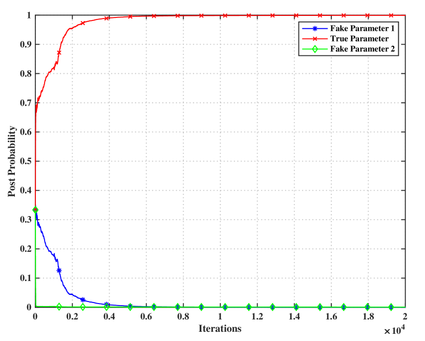
Figure 1: The average belief of five agents for three candidate parameters

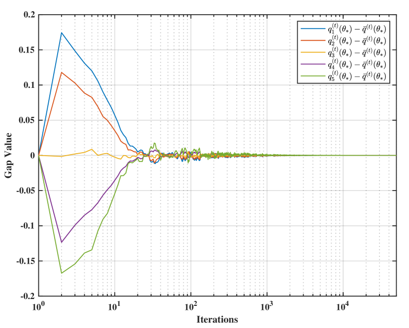
Figure 2: The gap between average belief and each agent’s belief of true parameter

Furthermore, the adaptive decision sequences of all agents are presented in Figure 3. We can see that five agents’ decision reach consensus to the true optimal decision.

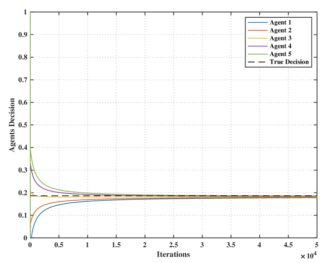
Figure 3: Decision convergence of all agents under Algorithm 1

The impact of stepsizes. Besides, we implement Algorithm 1 with different stepsizes to explore their impact on the algorithm convergence. The beliefs of the true parameter with stepsizes $\alpha^{(t)}=\frac{1}{t+3},\frac{1}{t+5},\frac{10}{t+80}$ are shown in Figure 5. Since $\frac{10}{t+80}>\frac{1}{t+3}>\frac{1}{t+5}$ for any $t\geq 6$, and $\sum_{t=1}^{T}\frac{10}{t+80}>\sum_{t=1}^{T}\frac{1}{t+3}>\sum_{t=1}^{T}\frac{1}{t+5}$ for any $T\geq 15$. Based on the convergence rate (58) of beliefs, we can obtain that as $T\rightarrow\infty$, algorithm implement with stepsize $\frac{10}{t+80}$ converge faster than others. Whereas at the beginning when $T$ is small, due to $\sum_{t=1}^{T}\frac{1}{t+3}>\sum_{t=1}^{T}\frac{10}{t+80}$, algorithm with stepsize $\frac{1}{t+3}$ performs better. The theoretical results match the numerical results in Figure 5. Generally speaking, algorithm with bigger stepsize leads to faster convergence rate as data information used is much more efficient than prior information due to Equation (2).

Different distributed consensus protocol comparison. We further carry out simulations to compare the classical distributed linear consensus protocol [31] with (3) which implements distributed consensus averaging on a reweighting of the log-belief. The result demonstrated in Figure 5 shows that the log-belief is faster than linear consensus, which is consistent with the theoretical discussions in Remark 2.

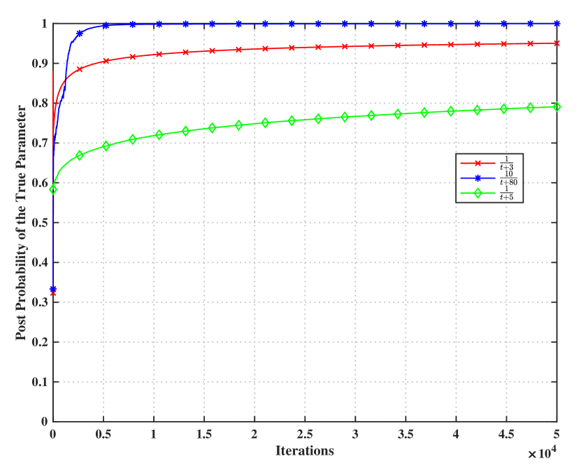
Figure 4: The impact of stepsizes on the convergence rate of the true parameter’s belief

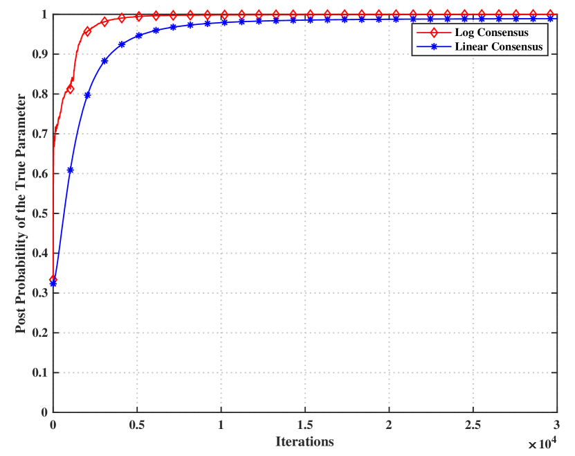
Figure 5: Comparison between log-belief and linear consensus

4.2 Source Research

In addition, we conduct experiments on the problem of an ideal source localization and cleanup for a pollution source. Consider distributed wireless sensor and actor networks (WSANs) with five devices that are capable of sampling water quality, processing the data, and making decisions of the source localization based on the observations.

Let $x=(x_{1},x_{2})$ denote the localization of sampling water and $\theta=(\beta_{1},\beta_{2})$ be the pollution source localization. Under stable source strength and static water conditions, the pollution source forms a stable field which is the Gauss model of continuous point source diffusion in unbounded space [36] that can be formulated as

$$c (x=(x_{1},x_{2});\theta=(\beta_{1},\beta_{2}))$$

$$=c_{0}\exp{\left(-\frac{(x_{1}-\beta_{1})^{2}}{2\sigma_{1}^{2}}-\frac{(x_{2}-\beta_{2})^{2}}{2\sigma_{2}^{2}}\right)},$$ (70)

where $c_{0}$ is the initial constant concentration of pollution source; $\sigma_{1}$ and $\sigma_{2}$ denote the lateral diffusion parameter and the longitudinal diffusion parameter, respectively.

Five WSAs try to find the source by optimizing the aggregation function collaboratively

$$\min_{x}\frac{1}{5}\sum_{i=1}^{5}-c_{i}(x;\theta_{*}).$$ (71)

where $c_{i}$ is defined in (70) with different $x_{i}$, which is the localization of different agents. The initial localizations of five WSAs are $(-2,0),(-0.5,3),(2,4),(4,-1),(1,-3)$, respectively. Three possible pollution source is $\theta_{1}=(0,0),\theta_{2}=(4,3),\theta_{3}=(2,-2)$, where $\theta_{*}=\theta_{1}$. Set $c_{0}=100,\sigma_{1}=\sigma_{2}=2$, and $\epsilon_{i}\sim N(0,1)$.

The five WSAs use Algorithms 1 to identify the true location of the target and adaptively move towards the center of the pollution source by sampling the water quality at their current location. The motion trajectories of the five participants are shown in Figure 6. It can be observed that all sensing and actuation devices first achieve consensus and then cooperatively locate the real pollution source. The experimental results align with theoretical analysis, indicating a faster convergence speed for consensus compared to the optimization convergence speed.

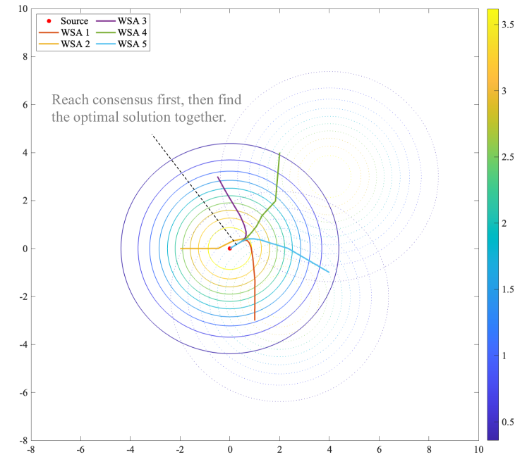
Figure 6: Motion trajectories of agents in sensor pollution clean problem

5 Conclusion

This work has provided valuable insights for addressing parameteric uncertainty in distributed optimization problems and simultaneously found the optimal solution. To be more specific, a general mathematical framework which considers learning the unknown parameter of model whereas adaptive distributed optimization has been considered, different from prior work with exact parametric structure. We have designed a novel distributed fractional Bayesian learning algorithm to resolve the bidirectional coupled problem. We then have proved that agents’ beliefs about the unknown parameter converge to a common belief, and that the decision variables also converge to the optimal solution almost surely. It is worth noting from the numerical experiments that by utilizing the consensus protocol which averages on a reweighting of the log-belief, we have attained faster than normal distributed linear consensus protocol. In future, it is of interests to adapt the proposed method into real-world situations, and further investigate the bidirectional coupled distributed optimization problems with continuous unknown model parameters.

References

6 Proof of Lemma 3

Proof.

With the definition (24), we obtain that

$$F_{i}(x,\boldsymbol{q}_{i}) =q_{i}(\theta_{1})J_{i}(x,\theta_{1})+\cdots+q_{i}(\theta_{M})J_{i}(x,\theta_{M}).$$ (72)

Then by recalling from Assumption 4 that for every $\theta_{m}$,

$$J_{i}(\lambda x+(1-\lambda)y,\theta_{m})\leq \lambda J_{i}(x,\theta_{m})+(1-\lambda)J_{i}(y,\theta_{m})$$

$$-\frac{\mu}{2}\lambda(1-\lambda)\|x-y\|^{2}.$$ (73)

Hence, for all $x,y\in\mathbb{R}$ and $\lambda\in(0,1)$.

$$F_{i}(\lambda x+(1-\lambda)y,\boldsymbol{q}_{i})\leq q_{i}(\theta_{1})\big{[}\lambda J_{i}(x,\theta_{1})+(1-\lambda)J_{i}(y,\theta_{1})$$

$$\quad-\frac{\mu}{2}\lambda(1-\lambda)\|x-y\|^{2}\big{]}+\cdots+q_{i}(\theta_{M})\big{[}\lambda J_{i}(x,\theta_{1})$$

$$\quad+(1-\lambda)J_{i}(y,\theta_{1})-\frac{\mu}{2}\lambda(1-\lambda)\|x-y\|^{2}\big{]}$$

$$=\lambda\Big{[}q_{i}(\theta_{1})J_{i}(x,\theta_{1})+\cdots+q_{i}(\theta_{m})J_{i}(x,\theta_{m})\Big{]}$$

$$\quad+(1-\lambda)\Big{[}q_{i}(\theta_{1})J_{i}(y,\theta_{1})+\cdots+q_{i}(\theta_{m})J_{i}(y,\theta_{m})\Big{]}$$

$$\quad-\big{(}q_{i}(\theta_{1})+\cdots+q_{i}(\theta_{m})\big{)}\frac{\mu}{2}\lambda(1-\lambda)\|x-y\|^{2}$$

$$=\lambda F_{i}(x,\boldsymbol{q}_{i})+(1-\lambda)F_{i}(y,\boldsymbol{q}_{i})-\frac{\mu}{2}\lambda(1-\lambda)\|x-y\|^{2}.$$

It indicates that $F_{i}(x,\boldsymbol{q}_{i})$ is strongly convex in $x$ with a constant $\mu$.

As for the properties of Lipschitz continuous gradients, by using Assumption 4, we derive from [37] that

$$\nabla_{x}^{2}J_{i}(x,\theta_{m})\leq L,\forall\theta_{m}\in\Theta,$$ (74)

Then

$$\nabla_{x}^{2}F_{i}(x,\boldsymbol{q}_{i}) =q_{i}(\theta_{1})\nabla_{x}^{2}J_{i}(x,\theta_{1})+\cdots+q_{i}(\theta_{M})\nabla_{x}^{2}J_{i}(x,\theta_{M})$$

$$\leq q_{i}(\theta_{1})L+\cdots+q_{i}(\theta_{M})L=L$$ (75)

where the last equality holds since the sum of belief is $1$.

7 Proof of Lemma 6

Proof.

For any $t\geq 0$, in order to bound $\|\boldsymbol{x}^{(t)}-\boldsymbol{1}x^{*}(\tilde{\boldsymbol{q}})\|^{2}$, we firstly consider bounding $\|x_{i}^{(t)}-\alpha^{(t)}\nabla_{x}F_{i}(x_{i}^{(t)},\boldsymbol{q}_{i}^{(t)})-x^{*}(\tilde{\boldsymbol{q}})\|^{2}$ for all $i\in\mathcal{N}$.

$$\|x_{i}^{(t)}-\alpha^{(t)}\nabla_{x}F_{i}(x_{i}^{(t)},\boldsymbol{q}_{i}^{(t)})-x^{*}(\tilde{\boldsymbol{q}})\|^{2}$$

$$=\|x_{i}^{(t)}-x^{*}(\tilde{\boldsymbol{q}})\|^{2}+[\alpha^{(t)}]^{2}\|\nabla_{x}F_{i}(x_{i}^{(t)},\boldsymbol{q}_{i}^{(t)})\|^{2}$$

$$~{}-2\alpha^{(t)}\nabla_{x}F_{i}(x_{i}^{(t)},\boldsymbol{q}_{i}^{(t)})^{T}(x_{i}^{(t)}-x^{*}(\tilde{\boldsymbol{q}}))$$

$$\leq\|x_{i}^{(t)}-x^{*}(\tilde{\boldsymbol{q}})\|^{2}+[\alpha^{(t)}]^{2}\|\nabla_{x}F_{i}(x_{i}^{(t)},\boldsymbol{q}_{i}^{(t)})\|^{2}$$

$$~{}-\!2\alpha^{(t)}\!\big{(}\nabla_{x}F_{i}(x_{i}^{(t)},\boldsymbol{q}_{i}^{(t)})\!-\!\nabla_{x}F_{i}(x^{*}(\tilde{\boldsymbol{q}}),\boldsymbol{q}_{i}^{(t)})\big{)}^{T}\!(x_{i}^{(t)}\!-x^{*}(\tilde{\boldsymbol{q}}))$$

$$~{}+2\alpha^{(t)}\|\nabla_{x}F_{i}(x^{*}(\tilde{\boldsymbol{q}}),\boldsymbol{q}_{i}^{(t)})\|\|x_{i}^{(t)}-x^{*}(\tilde{\boldsymbol{q}})\|$$

$$\leq(1-2\alpha^{(t)}\mu)\|x_{i}^{(t)}-x^{*}(\tilde{\boldsymbol{q}})\|^{2}+[\alpha^{(t)}]^{2}\|\nabla_{x}F_{i}(x_{i}^{(t)},\boldsymbol{q}_{i}^{(t)})\|^{2}$$

$$\quad+2\alpha^{(t)}\|\nabla_{x}F_{i}(x^{*}(\tilde{\boldsymbol{q}}),\boldsymbol{q}_{i}^{(t)})\|\|x_{i}^{(t)}-x^{*}(\tilde{\boldsymbol{q}})\|$$ (76)

where the last inequality follows by the strong convexity of $F_{i}(x,\boldsymbol{q})$ with $x$ in Lemma 3.

Then similarly to the derivation of (3.2) and (50), we have

$$\|\nabla_{x} F_{i}(x_{i}^{(t)},\boldsymbol{q}_{i}^{(t)})\|^{2}\leq$$

$$2M\|\nabla_{x}\boldsymbol{J}_{i}(x^{*}(\tilde{\boldsymbol{q}}),\boldsymbol{\theta})\|^{2}+2M^{2}L^{2}\|x_{i}^{(t)}-x^{*}(\tilde{\boldsymbol{q}})\|^{2}$$ (77)

and

$$\|\nabla_{x}F_{i}(x^{*}(\tilde{\boldsymbol{q}}),\boldsymbol{q}_{i}^{(t)})\|^{2}\leq M\|\nabla_{x}\boldsymbol{J}_{i}(x^{*}(\tilde{\boldsymbol{q}}),\boldsymbol{\theta})\|^{2}.$$ (78)

Substituting (77) and (78) into (76), we can obtain

$$\|x_{i}^{(t)}- \alpha^{(t)}\nabla_{x}F_{i}(x_{i}^{(t)},\boldsymbol{q}_{i}^{(t)})-x^{*}(\tilde{\boldsymbol{q}})\|^{2}$$

$$\leq(1-2\alpha^{(t)}\mu+2M^{2}L^{2}[\alpha^{(t)}]^{2})\|x_{i}^{(t)}-x^{*}(\tilde{\boldsymbol{q}})\|^{2}$$

$$~{}+2\alpha^{(t)}\|\nabla_{x}\boldsymbol{J}_{i}(x^{*}(\tilde{\boldsymbol{q}}),\boldsymbol{\theta})\|\sqrt{M}\|x_{i}^{(t)}-x^{*}(\tilde{\boldsymbol{q}})\|$$

$$~{}+2M[\alpha^{(t)}]^{2}\|\nabla_{x}\boldsymbol{J}_{i}(x^{*}(\tilde{\boldsymbol{q}}),\boldsymbol{\theta})\|^{2}.$$

Since $\{\alpha^{(t)}\}_{t\geq 0}$ is a decreasing stepsize to zero, then there exists a constant $T>0$ such that for all $t\geq T$, $\alpha^{(t)}\leq\frac{\mu}{2M^{2}L^{2}}$. Hence, for any $t\geq T$,

$$\|x_{i}^{(t)}- \alpha^{(t)}\nabla_{x}F_{i}(x_{i}^{(t)},\boldsymbol{q}_{i}^{(t)})-x^{*}(\tilde{\boldsymbol{q}})\|^{2}$$

$$\leq(1-\alpha^{(t)}\mu)\|x_{i}^{(t)}-x^{*}(\tilde{\boldsymbol{q}})\|^{2}$$

$$~{}+2\alpha^{(t)}\|\nabla_{x}\boldsymbol{J}_{i}(x^{*}(\tilde{\boldsymbol{q}}),\boldsymbol{\theta})\|\sqrt{M}\|x_{i}^{(t)}-x^{*}(\tilde{\boldsymbol{q}})\|$$

$$~{}+\alpha^{(t)}\frac{\mu}{ML^{2}}\|\nabla_{x}\boldsymbol{J}_{i}(x^{*}(\tilde{\boldsymbol{q}}),\boldsymbol{\theta})\|^{2}$$

$$\leq\|x_{i}^{(t)}-x^{*}(\tilde{\boldsymbol{q}})\|^{2}-\alpha^{(t)}\Big{[}\mu\|x_{i}^{(t)}-x^{*}(\tilde{\boldsymbol{q}})\|^{2}$$

$$~{}-2\sqrt{M}\|\nabla_{x}\boldsymbol{J}_{i}(x^{*}(\tilde{\boldsymbol{q}}),\boldsymbol{\theta})\|\|x_{i}^{(t)}-x^{*}(\tilde{\boldsymbol{q}})\|$$

$$~{}-\frac{\mu}{ML^{2}}\|\nabla_{x}\boldsymbol{J}_{i}(x^{*}(\tilde{\boldsymbol{q}}),\boldsymbol{\theta})\|^{2}\Big{]}.$$ (79)

Let us define

$$\mathcal{X}_{i}\triangleq\{p\geq 0:\mu p^{2} -2\sqrt{M}\|\nabla_{x}\boldsymbol{J}_{i}(x^{*}(\tilde{\boldsymbol{q}}),\boldsymbol{\theta})\|p$$

$$-\frac{\mu}{ML^{2}}\|\nabla_{x}\boldsymbol{J}_{i}(x^{*}(\tilde{\boldsymbol{q}}),\boldsymbol{\theta})\|^{2}\leq 0\},$$ (80)

which is non-empty and compact. If $\|x_{i}^{(t)}-x^{*}(\tilde{\boldsymbol{q}})\|\notin\mathcal{X}$, we conclude from (79) that

$$\|x_{i}^{(t)}-\alpha^{(t)}\nabla_{x}F_{i}(x_{i}^{(t)},\boldsymbol{q}_{i}^{(t)})-x^{*}(\tilde{\boldsymbol{q}})\|^{2}\leq\|x_{i}^{(t)}-x^{*}(\tilde{\boldsymbol{q}})\|^{2}.$$ (81)

Otherwise,

$$\|x_{i}^{(t)} -\alpha^{(t)}\nabla_{x}F_{i}(x_{i}^{(t)},\boldsymbol{q}_{i}^{(t)})-x^{*}(\tilde{\boldsymbol{q}})\|^{2}\leq$$

$$\max_{p\in\mathcal{X}_{i}}\Big{\{}p^{2}-\frac{\mu}{2M^{2}L^{2}}\big{[}\mu p^{2}-2\sqrt{M}\|\nabla_{x}\boldsymbol{J}_{i}(x^{*}(\tilde{\boldsymbol{q}}),\boldsymbol{\theta})\|p$$

$$-\frac{\mu}{ML^{2}}\|\nabla_{x}\boldsymbol{J}_{i}(x^{*}(\tilde{\boldsymbol{q}}),\boldsymbol{\theta})\|^{2}\big{]}\Big{\}}$$

$$=\max_{p\in\mathcal{X}_{i}}\Big{\{}(1-\tfrac{\mu^{2}}{2ML^{2}})p^{2}+\frac{\mu\|\nabla_{x}\boldsymbol{J}_{i}(x^{*}(\tilde{\boldsymbol{q}}),\boldsymbol{\theta})\|}{M^{1.5}L^{2}}p$$

$$\qquad+\frac{\mu^{2}\|\nabla_{x}\boldsymbol{J}_{i}(x^{*}(\tilde{\boldsymbol{q}}),\boldsymbol{\theta})\|^{2}}{2M^{3}L^{4}}\Big{\}}.$$ (82)

From the definition of $\mathcal{X}_{i}$ , the right zero point of the upward opening parabola in (80) is

$$p_{i}^{(r)}=\frac{1}{2\mu}\Bigg{(}2\sqrt{M}\|\nabla_{x}\boldsymbol{J}_{i}(x^{*}(\tilde{\boldsymbol{q}}),\boldsymbol{\theta})\|$$

$$+\sqrt{4M\|\nabla_{x}\boldsymbol{J}_{i}(x^{*}(\tilde{\boldsymbol{q}}),\boldsymbol{\theta})\|^{2}+\frac{4\mu^{2}}{ML^{2}}\|\nabla_{x}\boldsymbol{J}_{i}(x^{*}(\tilde{\boldsymbol{q}}),\boldsymbol{\theta})\|^{2}}\Bigg{)}$$

$$=\left(\frac{\sqrt{M}}{\mu}+\frac{2}{L}\sqrt{\frac{M^{2}L^{2}+1}{M}}\right)\|\nabla_{x}\boldsymbol{J}_{i}(x^{*}(\tilde{\boldsymbol{q}}),\boldsymbol{\theta})\|,$$ (83)

which means $\mathcal{X}_{i}=[0,p_{i}^{(r)}]$. Since the values of quadratic function is bounded in a bounded closed set, we define

$$\max_{p\in\mathcal{X}_{i}}\Big{\{}(1-\tfrac{\mu^{2}}{ML^{2}})p^{2}+\frac{\mu\|\nabla_{x}\boldsymbol{J}_{i}(x^{*}(\tilde{\boldsymbol{q}}),\boldsymbol{\theta})\|}{M^{1.5}L^{2}}p$$

$$\qquad+\frac{\mu^{2}\|\nabla_{x}\boldsymbol{J}_{i}(x^{*}(\tilde{\boldsymbol{q}}),\boldsymbol{\theta})\|^{2}}{2M^{3}L^{4}}\Big{\}}\triangleq R_{i}.$$ (84)

Combining (81) and (82), together with (84), we have

$$\|x_{i}^{(t)}- \alpha^{(t)}\nabla_{x}F_{i}(x_{i}^{(t)},\boldsymbol{q}_{i}^{(t)})-x^{*}(\tilde{\boldsymbol{q}})\|^{2}$$

$$\leq\max\{\|x_{i}^{(t)}-x^{*}(\tilde{\boldsymbol{q}})\|^{2},R_{i}\},\quad\forall t\geq T.$$ (85)

Recalling from the definition of $\boldsymbol{x}^{(t)}$ and $\mathbb{F}(\boldsymbol{x}^{(t)},\boldsymbol{Q}^{(t)})$ in (28) and (32) respectively, in light of relation (27) we have

$$\|\boldsymbol{x}^{(t+1)} -\boldsymbol{1}x^{*}(\tilde{\boldsymbol{q}})\|^{2}$$

$$=\|W\|^{2}\|\boldsymbol{x}^{(t)}-\alpha^{(t)}\mathbb{F}(\boldsymbol{x}^{(t)},\boldsymbol{Q}^{(t)})-\boldsymbol{1}x^{*}(\tilde{\boldsymbol{q}})\|^{2}$$

$$\leq\|\boldsymbol{x}^{(t)}-\alpha^{(t)}\mathbb{F}(\boldsymbol{x}^{(t)},\boldsymbol{Q}^{(t)})-\boldsymbol{1}x^{*}(\tilde{\boldsymbol{q}})\|^{2}$$

$$\overset{\eqref{bd-xi}}{\leq}\max\{\|\boldsymbol{x}^{(t)}-\boldsymbol{1}x^{*}(\tilde{\boldsymbol{q}})\|^{2},\sum_{i=1}^{N}R_{i}\},\quad\forall t\geq T,$$

where the first inequality holds by the $2$-norm of $W$ is $1$ from Assumption 2. As a result,

$$\|\boldsymbol{x}^{(t)}-\!\boldsymbol{1}x^{*}(\tilde{\boldsymbol{q}})\|^{2}\!\leq\!\max\Big{\{}\|\boldsymbol{x}^{(T)}-\boldsymbol{1}x^{*}(\tilde{\boldsymbol{q}})\|^{2},\sum_{i=1}^{N}R_{i}\Big{\}}.$$ (86)

Note that $\boldsymbol{x}^{(t+1)}=W\left(\boldsymbol{x}^{(t)}-\alpha^{(t)}\nabla_{x}\mathbb{F}\left(\boldsymbol{x}^{(t)},\boldsymbol{Q}^{(t)}\right)\right)$ from (27) based on the vector form of $\boldsymbol{x}$ and $\mathbb{F}$ in (28) and (32). Since each belief value $\boldsymbol{q}_{i}^{(t)}(\boldsymbol{\theta})$ is bounded by $1$ for all $t\geq 0$ and $i\in\mathcal{N}$, $\boldsymbol{Q}^{(t)}$ defined in (30) is bounded. This together with the continuity of $\nabla_{x}\mathbb{F}$ under Assumption 4, we conclude that for a fixed constant $T$, $\boldsymbol{x}^{(T)}$ is bounded. This together with (86) proves the lemma.

8 Proof of Lemma 7

Proof.

According to the recursion (52), we have

$$e^{(t+1)} \leq{\delta}^{t+1}e^{(0)}+c\sum_{\tau=0}^{t}{\delta}^{t-\tau}[\alpha^{(\tau)}]^{2}.$$

Since $\alpha^{(t)}$ is of order $\mathcal{O}(\frac{1}{t})$, without loss of generality we set $\alpha^{(t)}=\frac{\gamma}{t+T}$ with a constant $\gamma>0$ and $T>0$. Dividing both side of above inequality by $[\alpha^{(t)}]^{2}$, we have

$${e^{(t+1)}\over[\alpha^{(t)}]^{2}} \leq{{\delta}^{t+1}\over[\alpha^{(t)}]^{2}}e^{(0)}+c\sum_{\tau=0}^{t}{\delta}^{t-\tau}\left[{\alpha^{(\tau)}\over\alpha^{(t)}}\right]^{2}$$

$$=\underbrace{\frac{e^{(0)}}{\gamma^{2}}\cdot\frac{\delta^{t+1}}{\frac{1}{(t+T)^{2}}}}_{Term~{}4}+\underbrace{c\sum_{\tau=0}^{t}\delta^{t-\tau}\left(\frac{t+T}{\tau+T}\right)^{2}}_{Term~{}5}.$$ (87)

As for $Term~{}4$, since $\frac{1}{\delta}>1$ by $\delta\in(0,1)$, we can obtain that

$$\lim_{t\rightarrow\infty}\frac{\delta^{t+1}}{\frac{1}{(t+T)^{2}}}=\lim_{t\rightarrow\infty}\frac{(t+T)^{2}}{(\frac{1}{\delta})^{t}}=0.$$ (88)

As for $Term~{}5$, we have

$$Term~{}5 =c\sum_{\tau=0}^{t}\delta^{t-\tau}\left(1+\frac{t-\tau}{\tau+T}\right)^{2}$$

$$=c\sum_{\tau=0}^{t}\delta^{t-\tau}\left(1+\frac{2(t-\tau)}{\tau+T}+\frac{(t-\tau)^{2}}{(\tau+T)^{2}}\right)$$

$$\leq c\sum_{\tau=0}^{t}\delta^{\tau}+\frac{2c}{T}\sum_{\tau=1}^{t}\tau\delta^{\tau}+\frac{c}{T^{2}}\sum_{\tau=1}^{t}\tau^{2}\delta^{\tau}.$$ (89)

Since $\delta\in(0,1)$, we derive

$$\lim_{t\rightarrow\infty}\sum_{\tau=0}^{t}\delta^{\tau}=\frac{1}{1-\delta},$$ (90)

$$\lim_{t\rightarrow\infty}\sum_{\tau=1}^{t}\tau\delta^{\tau}=\delta\sum_{\tau=1}^{\infty}\tau\delta^{\tau-1}=\delta\left(\sum_{\tau=0}^{\infty}\delta^{\tau}\right)^{\prime}=\frac{\delta}{(1-\delta)^{2}}.$$ (91)

Moreover, due to

$$\left(\sum_{\tau=1}^{t}\delta^{\tau}\right)^{\prime\prime}=\sum_{\tau=2}^{t}\tau(\tau-1)\delta^{\tau-2}=\sum_{\tau=2}^{t}\tau^{2}\delta^{\tau-2}-\sum_{\tau=2}^{t}\tau\delta^{\tau-2},$$

we can obtain that

$$\sum_{\tau=1}^{t}\tau^{2}\delta^{\tau}=\delta^{2}\left[\left(\sum_{\tau=1}^{t}\delta^{\tau}\right)^{\prime\prime}+\frac{1}{\delta}\sum_{\tau=1}^{t}\tau\delta^{\tau-1}-1\right]+\delta,$$

and therefore

$$\lim_{t\rightarrow\infty}\sum_{\tau=1}^{t}\tau^{2}\delta^{\tau} =\delta^{2}\left[\frac{2}{(1-\delta)^{3}}+\frac{1}{\delta(1-\delta)^{2}}-1\right]+\delta$$

$$=\frac{\delta(1+\delta)}{(1-\delta)^{2}}+\delta(1-\delta).$$ (92)

Substituting (90), (91), and (92) into (89), we can get the upper bound of $Term~{}5$. Together with (88) of $Term~{}4$ and recalling (87), we acheive

$$0\leq\lim_{t\rightarrow\infty}\frac{e^{(t+1)}}{[\alpha^{(t)}]^{2}}\leq c\left[1+\frac{\delta^{2}(\delta+3)}{T^{2}(1-\delta)^{2}}+\frac{2\delta}{T^{2}(1-\delta)}\right].$$

Thus, $e^{(t+1)}=\mathcal{O}([\alpha^{(t)}]^{2})=\mathcal{O}(\frac{1}{t^{2}})$, which yields the conclusion.

References

- [1] Angelia Nedić. Distributed gradient methods for convex machine learning problems in networks: Distributed optimization. IEEE Signal Processing Magazine, 37(3):92–101, 2020.
- [2] Sulaiman A. Alghunaim and Ali H. Sayed. Distributed coupled multiagent stochastic optimization. IEEE Transactions on Automatic Control, 65(1):175–190, 2020.
- [3] Peter Trautman and Andreas Krause. Unfreezing the robot: Navigation in dense, interacting crowds. In 2010 IEEE/RSJ International Conference on Intelligent Robots and Systems, pages 797–803. IEEE, 2010.
- [4] Makram Chahine, Roya Firoozi, Wei Xiao, Mac Schwager, and Daniela Rus. Intention communication and hypothesis likelihood in game-theoretic motion planning. IEEE Robotics and Automation Letters, 8(3):1223–1230, 2023.
- [5] Gerard Cornuejols and Reha Tütüncü. Optimization methods in finance, volume 5. Cambridge University Press, 2006.
- [6] Craig Wilson, Venugopal V Veeravalli, and Angelia Nedić. Adaptive sequential stochastic optimization. IEEE Transactions on Automatic Control, 64(2):496–509, 2018.
- [7] Nam Ho-Nguyen and Fatma Kılınç-Karzan. Exploiting problem structure in optimization under uncertainty via online convex optimization. Mathematical Programming, 177(1-2):113–147, March 2018.
- [8] Simon Le Cleac’h, Mac Schwager, and Zachary Manchester. Lucidgames: Online unscented inverse dynamic games for adaptive trajectory prediction and planning. IEEE Robotics and Automation Letters, 6(3):5485–5492, 2021.
- [9] Graeme Best and Robert Fitch. Bayesian intention inference for trajectory prediction with an unknown goal destination. In 2015 IEEE/RSJ International Conference on Intelligent Robots and Systems (IROS), pages 5817–5823. IEEE, 2015.
- [10] Hao Jiang and Uday V Shanbhag. On the solution of stochastic optimization and variational problems in imperfect information regimes. SIAM Journal on Optimization, 26(4):2394–2429, 2016.
- [11] Necdet Serhat Aybat, Hesam Ahmadi, and Uday V Shanbhag. On the analysis of inexact augmented lagrangian schemes for misspecified conic convex programs. IEEE Transactions on Automatic Control, 67(8):3981–3996, 2021.
- [12] Hesam Ahmadi and Uday V Shanbhag. On the resolution of misspecified convex optimization and monotone variational inequality problems. Computational Optimization and Applications, 77(1):125–161, 2020.
- [13] Aswin Kannan, Angelia Nedić, and Uday V Shanbhag. Distributed stochastic optimization under imperfect information. 2015 54th IEEE Conference on Decision and Control (CDC), pages 400–405, 2015.
- [14] Ivano Notarnicola, Andrea Simonetto, Francesco Farina, and Giuseppe Notarstefano. Distributed personalized gradient tracking with convex parametric models. IEEE Transactions on Automatic Control, 68(1):588–595, 2023.
- [15] Nian Liu and Lei Guo. Stochastic adaptive linear quadratic differential games. arXiv preprint arXiv:2204.08869, 2022.
- [16] Angelia Nedić and Asuman Ozdaglar. Distributed subgradient methods for multi-agent optimization. IEEE Transactions on Automatic Control, 54(1):48–61, 2009.
- [17] Minghui Zhu and Sonia Martínez. On distributed convex optimization under inequality and equality constraints. IEEE Transactions on Automatic Control, 57(1):151–164, 2011.
- [18] Giuseppe Notarstefano, Ivano Notarnicola, and Andrea Camisa. Distributed optimization for smart cyber-physical networks. Foundations and Trends in Systems and Control, 7(3):253–383, 2020.
- [19] Hesam Ahmadi and Uday V Shanbhag. On the resolution of misspecified convex optimization and monotone variational inequality problems. Computational Optimization and Applications, 77(1):125–161, 2020.
- [20] Shijie Huang, Jinlong Lei, and Yiguang Hong. Distributed non-bayesian learning for games with incomplete information. arXiv preprint arXiv:2303.07212, 2023.
- [21] Manxi Wu, Saurabh Amin, and Asuman Ozdaglar. Multi-agent bayesian learning with adaptive strategies: Convergence and stability. arXiv preprint arXiv:2010.09128, 2020.
- [22] Pier Giovanni Bissiri, Chris C Holmes, and Stephen G Walker. A general framework for updating belief distributions. Journal of the Royal Statistical Society Series B: Statistical Methodology, 78(5):1103–1130, 2016.
- [23] Pooya Molavi, Alireza Tahbaz-Salehi, and Ali Jadbabaie. Foundations of non-bayesian social learning. Columbia Business School Research Paper, 2017.
- [24] Larry G Epstein, Jawwad Noor, and Alvaro Sandroni. Non-bayesian learning. The BE Journal of Theoretical Economics, 10(1):0000102202193517041623, 2010.
- [25] Anirban Bhattacharya, Debdeep Pati, and Yun Yang. Bayesian fractional posteriors. The Annals of Statistics, 1(2):209–230, 2019.
- [26] Anusha Lalitha, Tara Javidi, and Anand D Sarwate. Social learning and distributed hypothesis testing. IEEE Transactions on Information Theory, 64(9):6161–6179, 2018.
- [27] Shi Pu, Alex Olshevsky, and Ioannis Ch Paschalidis. A sharp estimate on the transient time of distributed stochastic gradient descent. IEEE Transactions on Automatic Control, 67(11):5900–5915, 2021.
- [28] Zifei Han, Keying Ye, and Min Wang. A study on the power parameter in power prior bayesian analysis. The American Statistician, 77(1):12–19, 2023.
- [29] Peter Grünwald. The safe bayesian: learning the learning rate via the mixability gap. International Conference on Algorithmic Learning Theory, pages 169–183, 2012.
- [30] Angelia Nedić, Alex Olshevsky, and César A Uribe. A tutorial on distributed (non-bayesian) learning: Problem, algorithms and results. 2016 IEEE 55th Conference on Decision and Control (CDC), pages 6795–6801, 2016.
- [31] Lin Xiao and Stephen Boyd. Fast linear iterations for distributed averaging. Systems & Control Letters, 53(1):65–78, 2004.
- [32] Daron Acemoglu, Munther A Dahleh, Ilan Lobel, and Asuman Ozdaglar. Bayesian learning in social networks. The Review of Economic Studies, 78(4):1201–1236, 2011.
- [33] Angelia Nedić, Asuman Ozdaglar, and Pablo A Parrilo. Constrained consensus and optimization in multi-agent networks. IEEE Transactions on Automatic Control, 55(4):922–938, 2010.
- [34] Yurii Nesterov. Introductory lectures on convex optimization: A basic course, volume 87. Springer Science & Business Media, 2013.
- [35] Konrad Knopp. Theory and Application of infinite series. Courier Corporation, 1990.
- [36] Yngvar Gotaas. A model of diffusion in a valley from a continuous point source. Archiv für Meteorologie, Geophysik und Bioklimatologie, Serie A, 21(1):13–26, 1972.
- [37] Léon Bottou, Frank E Curtis, and Jorge Nocedal. Optimization methods for large-scale machine learning. SIAM review, 60(2):223–311, 2018.