Transition between scattering regimes of 2D electron transport

Abstract

We examine 2D electron transport through a long narrow channel driven by an external electric field in presence of diffusive boundary scattering. At zero temperature, we derive an analytical solution of the transition from ballistic to diffusive transport if we increase the bulk disorder strength. This crossover yields characteristic current density profiles. Furthermore, we illustrate the current density in the transition from ballistic to hydrodynamic transport. This corresponds to the Gurzhi effect in the resistivity. We also study the influence of finite temperature on current densities and average current in this system. In particular, we analyze how different scaling laws of scattering with respect to temperature affect the current profile along the channel.

I Introduction

In recent years, the field of two dimensional (2D) electron transport has advanced remarkably [1, 2, 3, 4, 5, 6]. The emergence of ultraclean two dimensional materials like Ga(Al)As heterostructures, graphene or transition-metal dichalcogenides (TMDCs) has sparked developments both experimentally and theoretically [7, 8, 9, 10, 11, 12, 13, 14, 15, 16, 17, 18, 19, 20, 21, 22, 23, 24, 25]. In 2D systems, bulk scattering is less dominant than in their 3D counterparts, simply because there is less bulk. Consequently, it is possible to efficiently reduce impurity scattering in these systems. This possibility allows us to explore other than diffusive transport regimes in the laboratory, such as ballistic transport, hydrodynamic transport and their crossovers. Special focus lies on channel geometries as a setup for a 2D system with boundaries [7, 18, 19]. Particular transport regimes show characteristic flow profiles, which are observable in the laboratory [7, 26].
A theory of ballistic transport of a 2D electron gas in presence of electron-electron interactions in a channel has been developed in Ref. [18]. It has been predicted that the average current diverges logarithmically for weak electron-electron scattering. This divergence stems from longitudinal modes that do not scatter at the boundaries of the channel. We extend this analysis by different means: (i) We derive an analytical solution based on Meijer-G functions for the current density and the average current. (ii) We study the current density if we crossover between different transport regimes. (iii) We analyze the temperature dependence of transport for different scaling laws of 2D electron-electron scattering. The latter point is inspired by recent work [21, 27], where long-lived modes in 2D electron systems, have been proposed. These modes are characterized by scattering rates with particular power-law dependencies on the temperature T, i.e. $T^{\alpha}$ with $\alpha>2$. Kryhin and Levitov associate this behavior to non-Newtonian hydrodynamics [28].
This article is organized as follows. We introduce our model of a 2D electron system in a channel geometry in Sec. II. In Sec. III, we present the analytic solution for the current density and the average current describing the transition from ballistic to diffusive transport. In Sec. IV, we show current density profiles illustrating the transitions between different transport regimes (ballistic, diffusive, hydrodynamic). In Sec. V, we extend the theory to finite temperature. We pay particular attention to the temperature dependence of electron-electron scattering. We conclude in Sec. VI.

II Model

Figure 1: Schematic illustration of the 2D electron channel of width $W$ with an external electric field $E_{0}$ applied in longitudinal direction.

We consider 2D electron transport through a long but narrow sample of length $L$ and width $W$, where $L\gg W$, schematically illustrated in Fig. 1. We are interested in linear response to a homogeneous electric field $E_{0}$ along the sample in x-direction. The response is described by a non-equilibrium part in the distribution function $f$. Hence, the distribution function takes the form

$$f=f_{0}+\delta f,$$ (1)

where $f_{0}$ is the equilibrium Fermi distribution.
The distribution function depends on a number of parameters related to the setup, the applied field and the scattering mechanisms that we analyze in our work.
For the non-equilibrium part of the distribution function $\delta f$, it is common to use the ansatz

$$\delta f=\left(-\frac{\partial f_{0}}{\partial\epsilon}\right)h,$$ (2)

where $\epsilon$ is the electron energy. In semiclassics, which is the regime we are interested in, $f$ is a function of time, space and momentum $f(\vec{x},\vec{p},t)$. We directly drop the time-dependence as we want to study stationary solutions. Since we assume $L\gg W$, we also drop the $x$ dependence as our distribution should not depend on the longitudinal direction in this regime. This leaves us with $f=f(y,\vec{p})$. Next we introduce the angle $\varphi$, chosen as the angle of the electron velocity with the normal of the left sample edge, cf. Fig. 1. The electron velocity and therefore also the electron momentum is expressed through this angle via

$$\vec{p}=m\cdot\vec{v}=m\cdot v(\epsilon)\cdot\left(\begin{array}[]{c}\sin(\varphi)\\ \cos(\varphi)\end{array}\right),$$ (3)

where $m$ is the electron mass. The corresponding kinetic equation is given by

$$v(\epsilon)\left(\cos(\varphi)\frac{\partial h}{\partial y}-\sin(\varphi)eE_{0}\right)=St[h],$$ (4)

The collision integral $St[h]$ on the right handside of Eq. $\eqref{kineq1}$ includes electron-electron scattering and scattering due to disorder. We use a simplified form of the collision integral that satisfies these constraints [19, 17]:

$$St[h]=-\gamma h+\gamma_{ee}\hat{P}[h]+\gamma_{d}\hat{P}_{0}[h],$$ (5)

where $\gamma=\gamma_{d}+\gamma_{ee}$ is the total scattering rate and $\gamma_{ee}$ and $\gamma_{d}$ are the electron-electron and disorder scattering rates, respectively. $\hat{P}_{0}$ and $\hat{P}=\hat{P}_{-1}+\hat{P}_{0}+\hat{P}_{1}$ are projectors of $h(\varphi)$ onto the subspaces $\{1\}$ and $\{1,e^{\pm i\varphi}\}$. Since we consider zero magnetic field the terms proportional to $\hat{P}_{0}[h]$ vanish [19, 20]. In the analytical results presented below, we neglect the $\hat{P}[h]$ term, which is a reasonable approximation if the scattering rate is small [18]. However, we keep the $\hat{P}[h]$ term in our numerical analysis.
We assume diffusive boundary conditions , parametrized as

$$h(-W/2,\varphi) =c_{l}\;\;\;\;\;-\frac{\pi}{2}<\varphi<\frac{\pi}{2},$$ (6)

$$h(W/2,\varphi) =c_{r}\;\;\;\;\;\;\;\frac{\pi}{2}<\varphi<\frac{3\pi}{2}.$$ (7)

Here, $c_{l}$ and $c_{r}$ are quantities that correspond to the average value of the distribution function over all angles associated with electrons reflected from the respective other edge. They are defined as

$$c_{l} =-\frac{1}{2}\int_{\pi/2}^{3\pi/2}d\varphi^{\prime}\cos(\varphi^{\prime})h(-W/2,\varphi^{\prime}),$$ (8)

$$c_{r} =\frac{1}{2}\int_{-\pi/2}^{\pi/2}d\varphi^{\prime}\cos(\varphi^{\prime})h(W/2,\varphi^{\prime}).$$ (9)

Due to these boundary conditions, the probability of an electron being reflected on the sample edge is independent of the reflection angle $\varphi$ at a given boundary. Moreover, the transverse component of the electron flow vanishes at the edges and therefore, due to the continuity equation, everywhere. These considerations imply that $c_{l}+c_{r}=0$. For any antisymmetric function $h(\pm W/2,\varphi)$ in $\varphi$ this results in $c_{l}=c_{r}=0$.
Combining Eqs. $\eqref{kineq1}$ and $\eqref{collint}$ with the aforementioned approximation, we obtain the simplified kinetic equation

$$\cos(\varphi)\frac{\partial h}{\partial y}-eE_{0}\sin(\varphi)=-\gamma^{\prime}h,$$ (10)

where we define $\gamma^{\prime}=\frac{\gamma}{v(\epsilon_{F})}$. In Eq. (10), we replace $\epsilon$ by $\epsilon_{F}$ in the velocity $v(\epsilon)$, as we are interested in the low temperature regime, $k_{B}T\ll\epsilon_{F}$, for now. All the terms in Eq. (10) have the dimension [energy/length]. We divide the equation by $\left(\frac{\epsilon_{F}}{W}\right)$ to arrive at a dimensionless equation. Introducing the dimensionless variables

$$\hat{h} =\frac{h}{\epsilon_{F}}, \hat{E}_{0} =\frac{eE_{0}W}{\epsilon_{F}},$$

$$\hat{y} =\frac{y}{W}, \hat{\gamma} =\gamma^{\prime}W,$$

and inserting them into the kinetic equation, this yields

$$\cos(\varphi)\frac{\partial\hat{h}}{\partial\hat{y}}-\hat{E}_{0}\sin(\varphi)=-\hat{\gamma}\hat{h}\ ,$$ (11)

which we now analyze in detail.

III Crossover from ballistic to diffusive transport

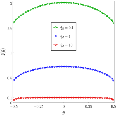
(a) testtestetstetstesttesttesttesttesttesttesttesttest

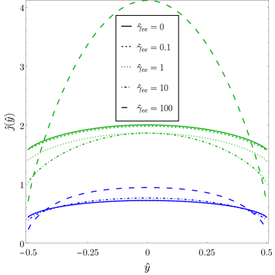
(b) testtestetstetstesttesttesttesttesttesttesttesttest

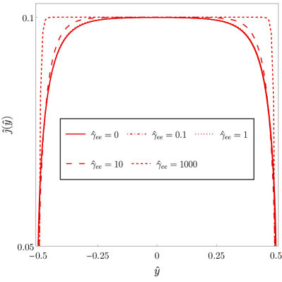
(c) testtestetstetstesttesttesttesttesttesttesttesttest

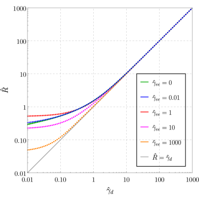
(d) testtestetstetstesttesttesttesttesttesttesttestte

Figure 2: (a) Transition from ballistic ($\hat{\gamma}_{d}=0.1$) to diffusive ($\hat{\gamma}_{d}=10$) transport in the current density $\hat{\jmath}(\hat{y})$. (b) Transition from ballistic to hydrodynamic transport as a function of $\hat{\gamma}_{ee}$ in the current density $\hat{\jmath}(\hat{y})$ for $\hat{\gamma}_{d}=0.1$ (green curves) and $\hat{\gamma}_{d}=1$ (blue curves). (c) Current density $\hat{\jmath}(\hat{y})$ for $\hat{\gamma}_{d}=10$ at different values of $\hat{\gamma}_{ee}$. (d) Resistance $\hat{R}=\frac{\hat{E_{0}}}{\hat{I}}$ as a function of $\hat{\gamma}_{d}$ at different $\hat{\gamma}_{ee}$.

It is straightforward to solve Eq. (11) with boundary conditions $\eqref{bc}$ [18]. The result can be written as

$$\hat{h}_{\pm}(\hat{y},\varphi)=\frac{\hat{E}_{0}\sin(\varphi)}{\hat{\gamma}}\left(1-\exp\left(-\frac{\hat{\gamma}(\hat{y}\pm\frac{1}{2})}{\cos(\varphi)}\right)\right),$$ (12)

where the index $\pm$ indicates the solution satisfying the boundary condition for the left and right edge respectively. We are interested in the current density $\hat{\jmath}(y)$ and the average current $\hat{I}$. The current density can be calculated via

$$\hat{\jmath}(\hat{y}) =\frac{1}{\pi}\int_{-\pi/2}^{\pi/2}\frac{\hat{E}_{0}\sin(\varphi)^{2}}{\hat{\gamma}}\left(1-\exp\left(-\frac{\hat{\gamma}(\hat{y}+\frac{1}{2})}{\cos(\varphi)}\right)\right)d\varphi$$ (13)

$$+\frac{1}{\pi}\int_{\pi/2}^{3\pi/2}\frac{\hat{E}_{0}\sin(\varphi)^{2}}{\hat{\gamma}}\left(1-\exp\left(-\frac{\hat{\gamma}(\hat{y}-\frac{1}{2})}{\cos(\varphi)}\right)\right)d\varphi$$

yielding

$$\hat{\jmath}(\hat{y}) =\frac{\hat{E}_{0}}{8\hat{\gamma}}\left(\sum_{\pm}(1\pm 2\hat{y})^{2}\hat{\gamma}^{2}\phantom{\frac{1}{2}}\right.$$ (14)

$$-\left.4\pi G_{2,4}^{2,0}\left(\frac{1}{16}(1\pm 2\hat{y})^{2}\hat{\gamma}^{2}|\begin{array}[]{c}0,2\\ \frac{1}{2},\frac{1}{2},0,0\\ \end{array}\right)\right),$$ (17)

where $G_{2,4}^{2,0}\left(\frac{1}{16}(1\pm 2\hat{y})^{2}\hat{\gamma}^{2}|\begin{array}[]{c}0,2\\ \frac{1}{2},\frac{1}{2},0,0\\ \end{array}\right)$ denotes the Meijer-G function. The average current associated with this current density takes the form

$$\hat{I}=\frac{\hat{E}_{0}W\hat{\gamma}}{3}-\frac{\pi\hat{E}_{0}W}{2\hat{\gamma}}G_{3,5}^{2,1}\left(\frac{\hat{\gamma}^{2}}{4}|\begin{array}[]{c}\frac{1}{2},0,2\\ \frac{1}{2},\frac{1}{2},-\frac{1}{2},0,0\\ \end{array}\right).$$ (18)

This result for the current is valid for any $\hat{\gamma}$ within the validity regime of Eq. (10). In the limit $\hat{\gamma}\rightarrow 0$, we obtain in leading order

$$\hat{I}=\frac{2W}{\pi}\left(\ln\left(\frac{1}{\hat{\gamma}}\right)+\ln(2)+\frac{1}{2}-\varGamma\right),$$ (19)

where $\varGamma$ is Euler’s constant. Note that Eq. (19) resembles Eq. (22) in Ref. [30].

IV Current density profiles

In the following, we present and analyze current density profiles for different transport regimes. Some results are based on analytical solutions of the previous section. Others are derived numerically.
In the limit $\hat{\gamma}\ll 1$, the current density (14) shows parabolic behaviour, illustrated in Fig. LABEL:sub@subfig:a. This feature is somewhat counter intuitive but known. It can be viewed as a current density that resembles the shape of hydrodynamic electron flow in weakly interacting systems (hydro without hydro). It stems from the combination of ballistic transport with diffusive boundary scattering. For $\hat{\gamma}>1$, we observe the transition to the diffusive regime, which has the characteristic flat form of the current density [25] due to dominant bulk-impurity scattering. This crossover from ballistic to diffusive transport is fully described by our analytical results.
Note that Eqs. (14) and (18) also describe transport regimes, in which electron-electron scattering is relevant as long as the corresponding scattering rate is weak enough, see Fig. LABEL:sub@subfig:b. With the numerical methods described in Ref. [31], we solve Eq. (4) taking into account all terms in the collision integral (5). These results contain two parameters $\hat{\gamma}_{ee}$ and $\hat{\gamma}_{d}$. We are able to reproduce the results of Ref. [30]. However, we go beyond these results by a careful comparison of the current densities if we crossover between different scattering regimes. The numerical results for $\hat{\gamma}_{ee}=0$ coincide with the analytical results given by Eqs. (14) and (18) .
In Fig. LABEL:sub@subfig:b, we show the transition from ballistic to hydrodynamic transport for two different values of $\hat{\gamma}_{d}$. We find that the transition to the hydrodynamic regime, characterized by the parabolic form of the current density, occurs only for smaller values of $\hat{\gamma}_{d}$. Instead, for larger values of $\hat{\gamma_{d}}$, impurity scattering in the bulk is dominant. This is most pronounced for $\hat{\gamma}_{d}\gg 1$, as illustrated in Fig. LABEL:sub@subfig:c. In this case, the current density can not take a parabolic form even for very large values of $\hat{\gamma}_{ee}\gg\hat{\gamma}_{d}$. Increasing the electron-electron scattering rate then just enhances the flat range of the current density. This phenomenon can also be observed in the resistance, which becomes linear for $\hat{\gamma}_{d}\gg 1$ for all values of $\hat{\gamma}_{ee}$, displayed in Fig. LABEL:sub@subfig:d. The linear behavior sets in earlier for stronger electron-electron scattering. This occurs because the strong scattering between electrons as well as electron-impurity scattering hinders the majority of electrons from undergoing diffusive scattering at the boundaries. Indeed, the characteristic time for diffusive transition across the channel is $\tau_{b}\approx W^{2}v_{F}^{-2}(\gamma_{d}+\gamma_{ee})$. Hence, the role of the boundaries becomes negligible in the limit $\tau_{b}\rightarrow\infty$, which can be achieved by tuning $\gamma_{ee}$ as well as $\gamma_{d}$.
In Fig. LABEL:sub@subfig:d, we illustrate non-monotonic variations of the resistance $\hat{R}$ for fixed values of $\hat{\gamma}_{d}$. For instance, for small values $\hat{\gamma}_{d}$, $\hat{R}$ first increases with increasing $\hat{\gamma}_{ee}$ (Knudsen effect) and then decreases with increasing $\hat{\gamma}_{ee}$ (Poiseuille effect). The crossover from Knudsen to Poiseuille as a function of $\hat{\gamma}_{ee}$ is known as the Gurzhi effect.

V Finite-temperature current affected by electron-electron scattering

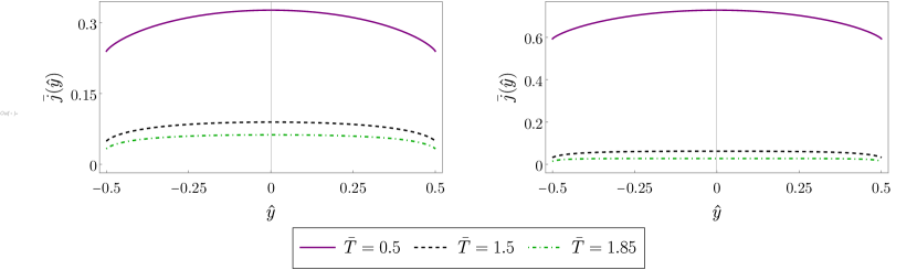
Figure 3: Current density $\bar{\jmath}(\hat{y})$ over $\hat{y}$ for $\alpha=2$ (left) and $\alpha=4$ (right) at different values of $\bar{T}$.

Next, we investigate the influence of finite temperature on average current and current density. We restrict ourselves to weak electron-electron scattering. Then, we can neglect the $P[\hat{h}]$ term in Eq. (5). We start with the solution to the kinetic equation displayed in Eq. (12) and reintroduce the energy dependence by $v(\epsilon)=\frac{\sqrt{2m\epsilon}}{m}$. This implies that we assume a quadratic dispersion relation of the electrons. In this section, we keep the physical dimension of the relevant parameters and observables of our model for now, to precisely consider the energy and temperature dependence of transport. Then, Eq. (12) is modified as

$$\tilde{h}_{\pm}(\tilde{y},\varphi,\epsilon)=\frac{\tilde{E}_{0}\sin(\varphi)\sqrt{2m\epsilon}}{\tilde{\gamma}\,m}\left(\!1-\exp\left(-\frac{\tilde{\gamma}(\tilde{y}\pm\frac{1}{2})m}{\cos(\varphi)\sqrt{2m\epsilon}}\right)\!\!\right)\!,$$ (20)

where $\tilde{E}_{0}=eE_{0}W$, $\tilde{\gamma}=\gamma W$ and $\tilde{y}=\frac{y}{W}$. The relevant integral for the current density is given by

$$\vec{j}(y)=2e\int\,\vec{v}\,\delta f\frac{d\vec{p}}{(2\pi\hbar)^{2}},$$ (21)

where $e$ is the elementary charge, $\vec{v}$ the velocity vector and $\delta f$ the nonequilibrium part of the distribution function. We use the same ansatz, $\delta f=\left(-\frac{\partial f_{0}}{\partial\epsilon}\right)\,\tilde{h}(\tilde{y},\varphi,\epsilon)$, as before. Next, we transform the momentum vector $\vec{p}$ to polar coordinates and switch from momentum to energy integration. This results in

$$\vec{j}(\tilde{y})=\int d\epsilon\int d\varphi\frac{e\sqrt{2m\epsilon}}{2\pi^{2}\hbar^{2}}\left(-\frac{\partial f_{0}}{\partial\epsilon}\right)\left(\begin{array}[]{c}\sin(\varphi)\\ \cos(\varphi)\end{array}\right)\tilde{h}(\tilde{y},\varphi,\epsilon).$$ (24)

We now address the current density that stems from charge carriers in an energy window around the Fermi energy $\epsilon_{F}$ of size $k_{B}T$, i.e.

$$\vec{j}(\tilde{y})=\frac{e}{2\pi^{2}\hbar^{2}}\int\limits_{\epsilon_{F}-\frac{k_{B}T}{2}}^{\epsilon_{F}+\frac{k_{B}T}{2}}\!\!\!\!\!d\epsilon\int\limits_{-\frac{\pi}{2}}^{{\frac{\pi}{2}}}d\varphi\frac{\sqrt{2m\epsilon}}{k_{B}T}\left(\begin{array}[]{c}\sin(\varphi)\\ \cos(\varphi)\end{array}\right)\tilde{h}(\tilde{y},\varphi,\epsilon).$$ (25)

The prefactor of $1/k_{B}T$ ensures that, in the limit $T\rightarrow 0$, the results of the previous section are recovered. Since the y-direction of the current density vanishes, we are left with $j_{x}(\tilde{y})$. We drop the x index in the following. Inserting $\tilde{h}_{+}(\tilde{y},\varphi,\epsilon)$ from Eq. (20), we obtain for $j_{+}(\tilde{y})$:

$$j_{+}(\tilde{y}) =\frac{e\tilde{E}_{0}}{\pi^{2}\hbar^{2}k_{B}T}\int\limits_{\epsilon_{F}-k_{B}T/2}^{\epsilon_{F}+k_{B}T/2}\!\!d\epsilon\int\limits_{-\frac{\pi}{2}}^{{\frac{\pi}{2}}}d\varphi\frac{\epsilon}{\gamma}\sin(\varphi)^{2}$$ (26)

$$\left(1-\exp\left(-\frac{\gamma(\tilde{y}+\frac{1}{2})m}{\cos(\varphi)\sqrt{2m\epsilon}}\right)\right).$$

Solving these integrals, the full current density $j(\tilde{y})=j_{+}(\tilde{y})+j_{-}(\tilde{y})$ can again be written in terms of the Meijer-G function as

$$j(\tilde{y})=\frac{e\tilde{E}_{0}m\tilde{\gamma}}{2\pi\hbar^{2}}\left(\frac{1}{4}+\tilde{y}^{2}\right)+\frac{e\tilde{E}_{0}m^{2}\tilde{\gamma}^{3}}{128\hbar^{2}k_{B}T}\cdot$$ (27)

$$\left[\left(\frac{1}{2}-\tilde{y}\right)^{4}\left(G_{2,4}^{2,0}\left(-\frac{m\tilde{\gamma}^{2}(\frac{1}{2}-\tilde{y})^{2}}{4(k_{B}T-2\epsilon_{F})}|\begin{array}[]{c}-2,1\\ -\frac{3}{2},-\frac{3}{2},-2,-2\\ \end{array}\right)\right.\right.$$ (30)

$$\left.\left.-G_{2,4}^{2,0}\left(\frac{m\tilde{\gamma}^{2}(\frac{1}{2}-\tilde{y})^{2}}{4(k_{B}T-2\epsilon_{F})}|\begin{array}[]{c}-2,1\\ -\frac{3}{2},-\frac{3}{2},-2,-2\\ \end{array}\right)\right)+\right.$$ (33)

$$\left.\left(\frac{1}{2}+\tilde{y}\right)^{4}\left(G_{2,4}^{2,0}\left(-\frac{m\tilde{\gamma}^{2}(\frac{1}{2}+\tilde{y})^{2}}{4(k_{B}T-2\epsilon_{F})}|\begin{array}[]{c}-2,1\\ -\frac{3}{2},-\frac{3}{2},-2,-2\\ \end{array}\right)\right.\right.$$ (36)

$$\left.\left.-G_{2,4}^{2,0}\left(\frac{m\tilde{\gamma}^{2}(\frac{1}{2}+\tilde{y})^{2}}{4(k_{B}T-2\epsilon_{F})}|\begin{array}[]{c}-2,1\\ -\frac{3}{2},-\frac{3}{2},-2,-2\\ \end{array}\right)\right)\right].$$ (39)

If we integrate the coordinate $y$ over the width of the channel, we arrive at the average current

$$I=\frac{e\tilde{E}_{0}Wm\tilde{\gamma}}{6\pi\hbar^{2}}+\frac{e\tilde{E}_{0}Wm^{2}\tilde{\gamma}^{3}}{128\hbar^{2}k_{B}T}\cdot$$ (40)

$$\left[G_{3,5}^{2,1}\left(-\frac{m\tilde{\gamma}^{2}}{4(T-2\epsilon_{F})}|\begin{array}[]{c}-\frac{3}{2},-2,1\\ -\frac{3}{2},-\frac{3}{2},-\frac{5}{2},-2,-2\\ \end{array}\right)\right.$$ (43)

$$\left.-G_{3,5}^{2,1}\left(\frac{m\tilde{\gamma}^{2}}{4(T+2\epsilon_{F})}|\begin{array}[]{c}-\frac{3}{2},-2,1\\ -\frac{3}{2},-\frac{3}{2},-\frac{5}{2},-2,-2\\ \end{array}\right)\right].$$ (46)

To plot these results, we introduce the dimensionless variables

$$\bar{\jmath} =\frac{\hbar W}{e\epsilon_{F}}j,\,\,\,\,\bar{I}=\frac{\hbar}{e\epsilon_{F}}I$$

$$\bar{\gamma}_{W} =\frac{m\tilde{\gamma}W}{\hbar},\,\,\,\,\bar{\gamma}_{F}^{2}=\frac{m\tilde{\gamma}^{2}}{\epsilon_{F}}$$ (47)

$$\bar{T} =\frac{k_{B}T}{\epsilon_{F}}\,\,\,\,\bar{E}_{0}=\frac{e\tilde{E}_{0}}{\epsilon_{F}}.$$

In the following, we assume that the scattering rate due to electron-electron scattering shows a power law scaling as a function of temperature:

$$\hat{\gamma}=C\left(k_{B}T\right)^{\alpha}.$$ (48)

This ansatz is inspired by recent works [21, 27, 28] on 2D transport. There, the authors argue that for certain modes a different scaling (other than $T^{2}$) can be expected. For simplicity, we assume a global $T^{\alpha}$ (for all modes). We investigate the influence of $\alpha$ on the current density and current. Inserting the ansatz into the dimensionless variables $\bar{\gamma}_{F}^{2}$ and $\bar{\gamma}_{W}$, we obtain

$$\bar{\gamma}_{F}^{2} =\frac{mC^{2}}{\epsilon_{F}}\left(k_{B}T\right)^{2\alpha}=\frac{mC^{2}\epsilon_{F}^{2\alpha}}{\epsilon_{F}}\left(\frac{k_{B}T}{\epsilon_{F}}\right)^{2\alpha}$$ (49)

$$=\underbrace{mC^{2}\epsilon_{F}^{2\alpha-1}}_{=C_{1}}\bar{T}^{2\alpha}=C_{1}\bar{T}^{2\alpha}$$

$$\bar{\gamma}_{W} =\frac{mWC}{\hbar}\left(k_{B}T\right)^{\alpha}=\frac{mWC\epsilon_{F}^{\alpha}}{\hbar}\left(\frac{k_{B}T}{\epsilon_{F}}\right)^{\alpha}$$ (50)

$$=\underbrace{\frac{mWC\epsilon_{F}^{\alpha}}{\hbar}}_{=C_{2}}\bar{T}^{\alpha}=C_{2}\bar{T}^{\alpha}$$ (51)

The final form of the dimensionless-$\bar{T}$-dependent current density and current then takes the form

$$\bar{\jmath}(\hat{y})=\frac{\bar{E}_{0}C_{2}\bar{T}^{\alpha}}{2\pi}\left(\frac{1}{4}+\hat{y}^{2}\right)+\frac{\bar{E}_{0}C_{1}C_{2}\bar{T}^{3\alpha-1}}{128}\cdot$$ (52)

$$\left[\left(\frac{1}{2}-\hat{y}\right)^{4}\left(G_{2,4}^{2,0}\left(\frac{C_{1}\bar{T}^{2\alpha}(\frac{1}{2}-\hat{y})^{2}}{4(2-\bar{T})}|\begin{array}[]{c}-2,1\\ -\frac{3}{2},-\frac{3}{2},-2,-2\\ \end{array}\right)\right.\right.$$ (55)

$$\left.\left.-G_{2,4}^{2,0}\left(\frac{C_{1}\bar{T}^{2\alpha}(\frac{1}{2}-\hat{y})^{2}}{4(2+\bar{T})}|\begin{array}[]{c}-2,1\\ -\frac{3}{2},-\frac{3}{2},-2,-2\\ \end{array}\right)\right)+\right.$$ (58)

$$\left.\left(\frac{1}{2}+\hat{y}\right)^{4}\left(G_{2,4}^{2,0}\left(\frac{C_{1}\bar{T}^{2\alpha}(\frac{1}{2}+\hat{y})^{2}}{4(2-\bar{T})}|\begin{array}[]{c}-2,1\\ -\frac{3}{2},-\frac{3}{2},-2,-2\\ \end{array}\right)\right.\right.$$ (61)

$$\left.\left.-G_{2,4}^{2,0}\left(\frac{C_{1}\bar{T}^{2\alpha}(\frac{1}{2}+\hat{y})^{2}}{4(2+\bar{T})}|\begin{array}[]{c}-2,1\\ -\frac{3}{2},-\frac{3}{2},-2,-2\\ \end{array}\right)\right)\right]$$ (64)

and

$$\bar{I}=\frac{\bar{E}_{0}WC_{2}\bar{T}^{\alpha}}{6\pi}+\frac{\bar{E}_{0}WC_{1}C_{2}\bar{T}^{3\alpha-1}}{128}\cdot$$ (65)

$$\left[G_{3,5}^{2,1}\left(\frac{C_{1}\bar{T}^{2\alpha}}{4(2-\bar{T})}|\begin{array}[]{c}-\frac{3}{2},-2,1\\ -\frac{3}{2},-\frac{3}{2},-\frac{5}{2},-2,-2\\ \end{array}\right)\right.$$ (68)

$$\left.-G_{3,5}^{2,1}\left(\frac{C_{1}\bar{T}^{2\alpha}}{4(2+\bar{T})}|\begin{array}[]{c}-\frac{3}{2},-2,1\\ -\frac{3}{2},-\frac{3}{2},-\frac{5}{2},-2,-2\\ \end{array}\right)\right].$$ (71)

In the latter equation, the term including the Meijer-G functions is of similar magnitude to the first term for $\bar{T}>1$. For $\bar{T}\ll 1$, the terms including the Meijer-G functions fully describe average current and current density. For $\bar{T}\ll 1$, current density and average current resemble their counterparts in the ballistic regime, see Fig. 3.
The average current $\bar{I}$ in the limit $\bar{T}\rightarrow 0$ is given by

$$\bar{I}=\frac{\sqrt{2}C_{2}W}{\pi^{2}\sqrt{C_{1}}}\left(\ln\left(\frac{\sqrt{2}}{\sqrt{C_{1}}\bar{T}^{\alpha}}\right)+\ln(2)+\frac{1}{2}-\varGamma\right)$$ (72)

similar to the zero temperature case stated in Eq. (19). This stems from the fact that the electrons do not have a phase space for scattering in this regime. In principle, Eq. (72) allows us to extract $\alpha$ in a clean system at small temperatures.
For $\alpha=0$, the current density and current are temperature-independent, displayed in Fig. 4. This is a non-trivial observation, as even for $\alpha=0$ some temperature dependence remains in the Meijer-G function but it cancels with the prefactor $1/\bar{T}$. The current and current density for $\alpha=0$ reproduce the zero temperature limit.

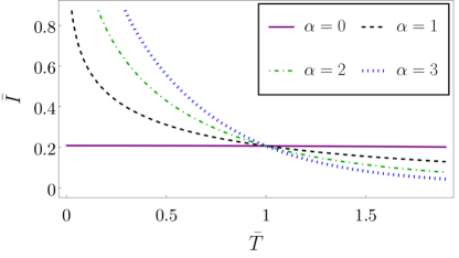
Figure 4: Current $\bar{I}$ over $\bar{T}$ for different values of $\alpha$. Note the change in the order for different $\alpha$ for $\bar{T}<1$ as compared to $\bar{T}>1$.

We expect that the ballistic regime $\bar{T}\ll 1$ is favored in conventional 2DEG systems with a large Fermi energy $\epsilon_{F}$ compared to the electron temperature. However, Dirac materials like graphene could realize the $\bar{T}>1$ regime close to the Dirac point.

VI Conclusions

We derive an analytical solution for the current density and average current at zero temperature that describes the transition from ballistic to diffusive transport. Furthermore, we carefully analyze the transition between different scattering regimes (ballistic, diffusive, hydrodynamic) numerically. We illustrate these transitions by characteristic current density profiles. We also predict temperature depending transport assuming temperature depending scattering. Our results could be used to extract the power law scaling of electron-electron scattering with respect to temperature for small temperatures compared to the Fermi energy.