Consisaug: A Consistency-based Augmentation for Polyp Detection in Endoscopy Image Analysis

Abstract

Colorectal cancer (CRC), which frequently originates from initially benign polyps, remains a significant contributor to global cancer-related mortality. Early and accurate detection of these polyps via colono-scopy is crucial for CRC prevention. However, traditional colonoscopy methods depend heavily on the operator’s experience, leading to suboptimal polyp detection rates. Besides, the public database are limited in polyp size and shape diversity. To enhance the available data for polyp detection, we introduce Consisaug, an innovative and effective methodology to augment data that leverages deep learning. We utilize the constraint that when the image is flipped the class label should be equal and the bonding boxes should be consistent. We implement our Consisaug on five public polyp datasets and at three backbones, and the results show the effectiveness of our method. All the codes are available at (https://github.com/Zhouziyuya/Consisaug).

1 Introduction

Colonoscopy, while essential for colorectal cancer (CRC) screening, is expensive, resource-demanding, and often met with patient reluctance. Unfortunately, up to 26% of colonoscopies may miss lesions and adenomas [1], as they heavily rely on the expertise of the endoscopist. In routine examinations, distinguishing between neoplastic and non-neoplastic polyps poses challenges, especially for less experienced endoscopists using current equipment [2] [3]. Besides, object detection labeling involves the expertise of the endoscopist assigning both a category and a bounding box location to each object in an image. This process is time-consuming, with an average of 10 seconds per object [4]. Consequently, object detection labeling incurs significant costs, demands extensive time commitments, and requires substantial effort.

Recently, there has been a great interest in deep learning in CRC screening. Various studies have developed models for automatic polyp segmentation [5] [6], polyp detection [7] [8] aiming to reduce the access barrier to pathological services. However, the deficiency of training data seriously impedes the development of polyp detection techniques. The existing fully-annotated databases, including CVC-ClinicDB[9], ETIS-Larib[10], CVC-ColonDB[11], Kvasir-Seg[12] and LDPolypVideo[13], are very limited in polyp size and shape diversity, which are far from the significant complexity in the actual clinical situation. Therefore, in this paper we want to find out an augmentation to fully use the dataset itself. By this motivation, we put forward an consistency-based augmentation to improve the performance of polyp detection which use Student-Teacher model to distill knowledge. Following we coarsely describe the consistency regularization and Student-Teacher model used in our architecture.

Consistency regularization is a method that has seen wide applications in semi-supervised learning, unsupervised learning, and self-supervised learning. The core idea behind consistency regularization is to encourage the model to produce similar outputs for similar inputs, thereby leveraging unlabeled data to improve generalization performance[14][15][16]. Student-Teacher models have been a focal point of research in the field of machine learning and specifically in the domain of knowledge distillation, where information is transferred from one machine learning model (the teacher) to another (the student). The objective is to leverage the capabilities of a large, complex model (the teacher) and distill this knowledge into a smaller, simpler model (the student), thereby optimizing computational efficiency without compromising the performance significantly [17] [18].

Through this work, we have made the following contributions:

• We propose a straightforward yet effective augmentation scheme that take advantage of the polyp image’s intrinsic flipping consistency property;

• We novelly combine flipping consistency with Student-Teacher architecture which show great effectiveness in polyp detection;

• The proposed consistency constraint augmentation for polyp detection works well on multiple datasets and backbones and effective for not only in-domain samples but cross-domain samples.

2 Method

The Consisaug to be presented works similarly depending on whether it is for a CNN-based or a transformer-based object detector. The overall structure is depicted in Fig. 1. The proposed structure is the combination of the Student-Teacher model and an object detection algorithm. To allow one-to-one correspondence of target objects, an original image $I$ is added to initial augmentation to get image $x$. And $x$ is added to our flipping augmentations to get the flip one $x^{\prime}$. As shown in Fig. 1, a paired bounding box should represent the same class and their localization information should be consistent.

In the Student branch, the labeled samples are trained using supervised loss in typical object detection approaches. The consistency loss is additionally used to combine the two outputs of the teacher and student model. In this section, the Student-Teacher model, consistency loss for localization and for classification will be introduced respectively.

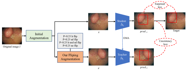
Figure 1: Overall structure of our proposed method.

2.1 The Student-Teacher Model

The framework of Consisaug used for this work shares the same overall structure as recent knowledge distillation approaches. There are two parts of the model Student and Teacher shown in Fig. 1. The Student model outputs predictions $f(I)$ of input images: $f(I)\triangleq f_{\theta_{s}}(I)$ and the same as Teacher model: $f(\hat{I})\triangleq f_{\theta_{t}}(\hat{I})$, $f(I)$ and $f(\hat{I})$ are a paired of bounding boxes which should represent the same class and consistent localization, $I$ and $\hat{I}\in{R}^{C\times H\times W}$ are the two input images of the models after respective augmentations. Differently, in the student branch, the original image $I_{0}$ will be randomly added initial augmentation including addnoise, multi-scale, flip and etc to get image $I$, while in the teacher branch, $I$ will be randomly added our flipping augmentations. The two models have the same architecture and the same initial weight. Besides, the weights of Student $\theta_{s}$ are updated by back-propagation and the weights of Teacher $\theta_{t}$ are updated by exponential moving average as Eq. 1. More precisely, the temperature $\tau\in[0,1]$ is given and updated after each iteration.

$$\theta_{t}\leftarrow\tau\theta_{s}+(1-\tau)\theta_{t}$$ (1)

2.2 Consistency loss for localization

We denote $f_{loc}^{k}(I)$ as the output localization of the rediction box. The localization result for the $k$-th candidate box $f_{loc}^{k}(I)$ consists of $[\Delta cx,\Delta cy,\Delta w,\Delta h]$, which represent the displacement of the center and scale coefficient of a candidate box, respectively. The output $f_{loc}^{k}(I)$ and its flipping version $f_{loc}^{k}(\hat{I})$ require a simple modification to be equivalent to each other. Since our flipping transformations make the coordinate offset move into the opposite direction, a negation should be applied to correct them. And we take the left and right flipping as an example in Eq. 2

$$\Delta cx^{k} \Longleftrightarrow-\Delta c\hat{x}^{k^{\prime}}$$ (2)

$$\Delta cy^{k},\Delta w^{k},\Delta h^{k} \Longleftrightarrow\Delta cyy^{k^{\prime}},\Delta\hat{w}^{k^{\prime}},\Delta\hat{h}^{k^{\prime}}$$

The localization consistency loss used for a single pair of bounding boxes in our method is given as below:

$$l_{con\_loc}(f_{loc}^{k}(I),f_{loc}^{k^{\prime}}(\hat{I}))= \frac{1}{4}\left(\left\|\Delta cx^{k}-\left(-\Delta\hat{cx}\hat{x}^{k^{\prime}}\right)\right\|^{2}+\left\|\Delta cy^{k}-\Delta\hat{cy}\hat{k}^{k^{\prime}}\right\|^{2}\right.$$ (3)

$$\left.+\left\|\Delta w^{k}-\Delta\hat{w}^{k^{\prime}}\right\|^{2}+\left\|\Delta h^{k}-\Delta\hat{h}^{k^{\prime}}\right\|^{2}\right)$$

The overall consistency loss for localization is then obtained from the average of loss values from all bounding box pairs:

$$\mathcal{L}_{con-l}=\mathbb{E}_{k}\left[l_{con\_loc}\left(f_{loc}^{k}(I),f_{loc}^{k^{\prime}}(\hat{I})\right)\right]$$ (4)

2.3 Consistency loss for classification

As for consistency loss for classification, we use Jensen-Shannon divergence (JSD) instead of the $L_{2}$ distance as the consistency regularization loss. $L_{2}$ distance treats all the classes equal, while in our flipping consistency circumstance irrelevant classes with low probability should not effect the classification performance much. JSD is a weaker constraint loss which is suitable in the consistency setting. The classification consistency loss is defined as below:

$$l_{con\_cls}\left(f_{cls}^{k}(I),f_{cls}^{k^{\prime}}(\hat{I})\right)=JS\left(f_{cls}^{k}(I),f_{cls}^{k^{\prime}}(\hat{I})\right)$$ (5)

where $JS$ denotes Jensen-Shannon divergence and $f_{cls}^{k}(I)$ is the model prediction class of the $k$-th box in image $I$. The overall consistency loss for classification of a pair of flipping images can be clarified as:

$$\mathcal{L}_{con-c}=\mathbb{E}_{k}\left[l_{con\_cls}\left(f_{cls}^{k}(I),f_{cls}^{k^{\prime}}(\hat{I})\right)\right]$$ (6)

The total consistency loss is the sum of location and classification consistency loss:

$$\mathcal{L}_{con}=\mathcal{L}_{con-l}+\mathcal{L}_{con-c}$$ (7)

Consequently, the final loss $\mathcal{L}$ is composed of the original object detector’s fully supervised loss $\mathcal{L}_{s}$ and our consistency loss $\mathcal{L}_{con}$:

$$\mathcal{L}=\mathcal{L}_{s}+\mathcal{L}_{con}$$ (8)

3 Experiments and Results

3.1 Implementation Details

Datasets and Baselines. Experiments are conducted on 5 public polyp datasets LDPolypVideo[13], CVC-ColonDB[11], CVC-ClinicDB[9], Kvasir-Seg[12] and ETIS-Larib[10]. The first one is the largest-scale challenging colonoscopy polyp detection dataset and the others are standard benchmarks for polyp segmentation. We summarize the 5 datasets by listing their parameters in Table 1. We use the official train test split on LDPolypVideo dataset and split 10% data from train set for validation. As for datasets with no officially released partition, we split 80% for training and 10% for validating and testing respectively.

We train our Consisaug on three baseline models to evaluate the effectiveness of our method: yolov5[19], SSD[20] and detr[21]. The first two are CNN-based models and the third one is Transformer-based model. All experiments have been done under the similar setting of the official codes and both codes are implemented based on Pytorch. The evaluation metrics used in our experiments are recall, precision, mAP50, F1-score, F2-score and the last three is vital in image detection. In detail, we use AdamW [22] optimizer with a cosine learning rate schedule, linear warm up of 10 epochs while the overall epoch is 100, and 0.0001 for the maximum learning rate value. The batch size is 32 and the image size is 640. We train with single Nvidia RTX3090 24G GPU to proceed each experiment.

Table 1: Summary of public annotated colonoscopy datasets.

Dataset	Label	Resolution	$N_{images}$	$N_{videos}$	$N_{polyps}$
LDPolypVideo	Bounding box	$560\times 480$	33884	160	200
CVC-ClinicDB	Mask	$384\times 288$	612	29	29
CVC-ColonDB	Mask	$574\times 500$	380	15	15
ETIS-Larib	Mask	$1225\times 966$	196	34	44
Kvasir-Seg	Mask	Various	1000	N/A	N/A

3.2 Results

Consisaug outperforms the vanilla version on different backbones. To demonstrate the effectiveness of our method, we train the polyp detection on three backbones yolov5[19], SSD[20], and DETR[21], and all are trained on the LDPolypVideo dataset[13], which has the largest size and diversity among the publicly released polyp datasets. The vanilla version model is trained using the official code and hyper-parameters, while the Consisaug version is trained using our method, which is reconstructed with the student-teacher model and our consistency-based augmentation. The results are shown in Table 2. All methods are trained three times, and the best results for each baseline are bolded. From the results, we can conclude that our Consisaug can enhance the polyp detection not only on CNN-based backbones (yolov5, SSD) but transformer-based backbone (DETR) from the three evaluation indexes mAP50, F1-score, and F2-score. Moreover, our method can also improve the recall, which is vital for lesion detection in medical image analysis.

Table 2: The polyp detection results on LDPolypVideo dataset. The best results for each baseline are bolded.

Baseline	Method	Recall	Precision	mAP50	F1-score	F2-score
yolov5	Vanilla	0.378$\pm$0.008	0.578$\pm$0.012	0.510$\pm$0.017	0.457$\pm$0.010	0.406$\pm$0.007
	Consisaug	0.453$\pm$0.004	0.575$\pm$0.015	0.540$\pm$0.024	0.507$\pm$0.018	0.473$\pm$0.011
SSD	Vanilla	0.658$\pm$0.028	0.152$\pm$0.006	0.515$\pm$0.013	0.248$\pm$0.009	0.396$\pm$0.011
	Consisaug	0.667$\pm$0.024	0.155$\pm$0.003	0.527$\pm$0.014	0.251$\pm$0.010	0.401$\pm$0.006
DETR	Vanilla	0.584$\pm$0.026	0.446$\pm$0.013	0.468$\pm$0.011	0.506$\pm$0.017	0.550$\pm$0.016
	Consisaug	0.629$\pm$0.030	0.480$\pm$0.013	0.504$\pm$0.015	0.544$\pm$0.016	0.592$\pm$0.022

Consisaug shows effectiveness on different colonoscopy datasets. To further verify the validity of our Consisaug method, we train the vanilla version and our Consisaug on other datasets. All the experiments are implemented on yolov5, and the results are shown in Table 3. Consisaug outperforms the vanilla version in at least four mAP50, F1-score, and F2-score metrics on five datasets.

Table 3: The polyp detection results based on yolov5 baseline for different datasets. The best results for each dataset are bolded.

Dataset	Method	Precision	Recall	mAP50	F1-score	F2-score
LDPolypVideo	Vanilla	0.378$\pm$0.008	0.578$\pm$0.012	0.510$\pm$0.017	0.457$\pm$0.010	0.406$\pm$0.007
	Consisaug	0.453$\pm$0.004	0.575$\pm$0.015	0.540$\pm$0.024	0.507$\pm$0.018	0.473$\pm$0.011
CVC-ClinicDB	Vanilla	0.933$\pm$0.002	0.781$\pm$0.006	0.865$\pm$0.009	0.850$\pm$0.003	0.807$\pm$0.007
	Consisaug	0.967$\pm$0.002	0.932$\pm$0.013	0.963$\pm$0.004	0.949$\pm$0.011	0.939$\pm$0.015
CVC-ClolonDB	Vanilla	0.997$\pm$0.003	0.789$\pm$0.013	0.891$\pm$0.005	0.881$\pm$0.007	0.823$\pm$0.001
	Consisaug	0.970$\pm$0.001	0.842$\pm$0.001	0.916$\pm$0.002	0.901$\pm$0.004	0.865$\pm$0.001
ETIS-Larib	Vanilla	0.982$\pm$0.003	0.350$\pm$0.005	0.634$\pm$0.009	0.516$\pm$0.007	0.402$\pm$0.003
	Consisaug	0.800$\pm$0.0005	0.450$\pm$0.012	0.629$\pm$0.003	0.576$\pm$0.002	0.493$\pm$0.004
Kvasir-Seg	Vanilla	0.937$\pm$0.006	0.730$\pm$0.008	0.848$\pm$0.001	0.821$\pm$0.007	0.764$\pm$0.002
	Consisaug	0.879$\pm$0.003	0.762$\pm$0.002	0.857$\pm$0.005	0.816$\pm$0.002	0.783$\pm$0.006

Consisaug transcends the vanilla version on cross-domain datasets. We also validate our method on cross-domain colonoscopy datasets detection. The vanilla and Consisaug versions are all trained on LDPolypVideo dataset yolov5 backbone. We test the two checkpoints on the other four whole datasets and the results are shown in Table 4. The results show the transferability of our model which is trained on one domain and tested on the other domains. Our method’s performance exceeds the vanilla version on all datasets from the metric of mAP50 and surpasses the vanilla version on three datasets from the F1-score and F2-score.

Table 4: Cross-domain polyp detection results. The four different datasets are test using vanilla yolov5 model and our Consisaug yolov5 model. The two models are all trained on LDPolypVideo dataset. The best results for each dataset are bolded.

Dataset	Method	Precision	Recall	mAP50	F1-score	F2-score
CVC-ClinicDB	Vanilla	0.783	0.598	0.716	0.678	0.628
	Consisaug	0.782	0.652	0.746	0.711	0.674
CVC-ClolonDB	Vanilla	0.780	0.578	0.701	0.664	0.610
	Consisaug	0.769	0.639	0.721	0.698	0.661
ETIS-Larib	Vanilla	0.725	0.625	0.713	0.671	0.643
	Consisaug	0.852	0.548	0.719	0.667	0.590
Kvasir-Seg	Vanilla	0.706	0.638	0.707	0.670	0.651
	Consisaug	0.755	0.632	0.736	0.688	0.653

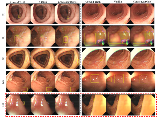
Figure 2: There are three columns for each image set. The first column is the image with ground truth, the second column shows the detection results of vanilla model and the third column is the results of our Consisaug method. The qualitative results prove that our Consisaug can (a) detect small targets, (b) detect targets in motion blur and reflections images, (c) detect targets between colon folds, (d) reduce false positive samples. And in (e) there will also be some failure cases for the hard detecting polyps.

Qualitative Results. In Fig. 2, we provide the polyp detection results of our Consisaug on LDPolypVideo test set. Our method can locate the polyp tissues in many challenging cases, such as small targets, motion blur and reflection images, polyps between colon folds, etc. But there are also some failure cases detection for the low image quality or the targets hidden in the dark.

4 Ablation Study

Table 5: The ablation study results on LDPolypVideo dataset yolov5 baseline. The best results for each baseline are bolded.

Sup loss	Consisaug	Flip aug	Recall	Precision	mAP50	F1-score	F2-score
✓	✗	✗	0.364$\pm$0.004	0.589$\pm$0.002	0.501$\pm$0.001	0.450$\pm$0.003	0.394$\pm$0.007
✓	✗	✓	0.378$\pm$0.008	0.578$\pm$0.012	0.510$\pm$0.017	0.457$\pm$0.010	0.406$\pm$0.007
✓	✓	✗	0.386$\pm$0.008	0.554$\pm$0.003	0.515$\pm$0.003	0.455$\pm$0.009	0.411$\pm$0.011
✓	✓	✓	0.453$\pm$0.004	0.575$\pm$0.015	0.540$\pm$0.014	0.507$\pm$0.018	0.473$\pm$0.011

In this section, we test the component of our Consisaug to provide deeper insight into our model. The supervised loss with flipping augmentations shown in Table 5 is the vanilla version used in section 3.2. The ablation studies can be split into four combinations: (a) the model only uses supervised loss; (b) the model uses supervised loss and flipping augmentations; (c) the model uses supervised loss combining with our Consisaug and (d) the model uses supervised loss, flipping augmentations and Consisaug. Comparing (b) and (c) we can infer that our flipping consistency augmentation Consisaug is more effective than the pure flipping augmentations. And from the results in (d), combining our Consisaug with flipping augmentations can get the best performance which further proves the validity of our method.

5 Conclusion

We propose Consisaug, a novel Student-Teacher based augmentation for lesion detection task. Our approach takes advantage of the characteristics of colonoscopic surgery, in which the lens can be rotated at any angle in the body so the flip of the colonoscopy picture at any angle is the image state that can be obtained. Therefore, we leverage the peculiarity of the colonscopies and the flip detecting consistency to prove our method. Extensive experiments demonstrate that Consisaug is a valid augmentation across five datasets and three backbones.

References

- [1] Shengbing Zhao, Shuling Wang, Peng Pan, Tian Xia, Xin Chang, Xia Yang, Liliangzi Guo, Qianqian Meng, Fan Yang, Wei Qian, et al. Magnitude, risk factors, and factors associated with adenoma miss rate of tandem colonoscopy: a systematic review and meta-analysis. Gastroenterology, 156(6):1661–1674, 2019.
- [2] Vaibhav Wadhwa, Muthuraman Alagappan, Adalberto Gonzalez, Kapil Gupta, Jeremy R Glissen Brown, Jonah Cohen, Mandeep Sawhney, Douglas Pleskow, and Tyler M Berzin. Physician sentiment toward artificial intelligence (ai) in colonoscopic practice: a survey of us gastroenterologists. Endoscopy international open, 8(10):E1379–E1384, 2020.
- [3] Barham K Abu Dayyeh, Nirav Thosani, Vani Konda, Michael B Wallace, Douglas K Rex, Shailendra S Chauhan, Joo Ha Hwang, Sri Komanduri, Michael Manfredi, John T Maple, et al. Asge technology committee systematic review and meta-analysis assessing the asge pivi thresholds for adopting real-time endoscopic assessment of the histology of diminutive colorectal polyps. Gastrointestinal endoscopy, 81(3):502–e1, 2015.
- [4] Olga Russakovsky, Li-Jia Li, and Li Fei-Fei. Best of both worlds: human-machine collaboration for object annotation. In Proceedings of the IEEE conference on computer vision and pattern recognition, pages 2121–2131, 2015.
- [5] Nikhil Kumar Tomar, Annie Shergill, Brandon Rieders, Ulas Bagci, and Debesh Jha. Transresu-net: Transformer based resu-net for real-time colonoscopy polyp segmentation. arXiv preprint arXiv:2206.08985, 2022.
- [6] Deng-Ping Fan, Ge-Peng Ji, Tao Zhou, Geng Chen, Huazhu Fu, Jianbing Shen, and Ling Shao. Pranet: Parallel reverse attention network for polyp segmentation. In International conference on medical image computing and computer-assisted intervention, pages 263–273. Springer, 2020.
- [7] Xinzi Sun, Dechun Wang, Qilei Chen, Jing Ni, Shuijiao Chen, Xiaowei Liu, Yu Cao, and Benyuan Liu. Maf-net: Multi-branch anchor-free detector for polyp localization and classification in colonoscopy. In International Conference on Medical Imaging with Deep Learning, pages 1162–1172. PMLR, 2022.
- [8] Yuncheng Jiang, Zixun Zhang, Ruimao Zhang, Guanbin Li, Shuguang Cui, and Zhen Li. Yona: You only need one adjacent reference-frame for accurate and fast video polyp detection. arXiv preprint arXiv:2306.03686, 2023.
- [9] Jorge Bernal, F Javier Sánchez, Gloria Fernández-Esparrach, Debora Gil, Cristina Rodríguez, and Fernando Vilariño. Wm-dova maps for accurate polyp highlighting in colonoscopy: Validation vs. saliency maps from physicians. Computerized medical imaging and graphics, 43:99–111, 2015.
- [10] Juan Silva, Aymeric Histace, Olivier Romain, Xavier Dray, and Bertrand Granado. Toward embedded detection of polyps in wce images for early diagnosis of colorectal cancer. International journal of computer assisted radiology and surgery, 9:283–293, 2014.
- [11] Jorge Bernal, Javier Sánchez, and Fernando Vilarino. Towards automatic polyp detection with a polyp appearance model. Pattern Recognition, 45(9):3166–3182, 2012.
- [12] Hanna Borgli, Vajira Thambawita, Pia H Smedsrud, Steven Hicks, Debesh Jha, Sigrun L Eskeland, Kristin Ranheim Randel, Konstantin Pogorelov, Mathias Lux, Duc Tien Dang Nguyen, et al. Hyperkvasir, a comprehensive multi-class image and video dataset for gastrointestinal endoscopy. Scientific data, 7(1):283, 2020.
- [13] Yiting Ma, Xuejin Chen, Kai Cheng, Yang Li, and Bin Sun. Ldpolypvideo benchmark: a large-scale colonoscopy video dataset of diverse polyps. In Medical Image Computing and Computer Assisted Intervention–MICCAI 2021: 24th International Conference, Strasbourg, France, September 27–October 1, 2021, Proceedings, Part V 24, pages 387–396. Springer, 2021.
- [14] Samuli Laine and Timo Aila. Temporal ensembling for semi-supervised learning. arXiv preprint arXiv:1610.02242, 2016.
- [15] Antti Tarvainen and Harri Valpola. Mean teachers are better role models: Weight-averaged consistency targets improve semi-supervised deep learning results. Advances in neural information processing systems, 30, 2017.
- [16] Takeru Miyato, Shin-ichi Maeda, Masanori Koyama, and Shin Ishii. Virtual adversarial training: a regularization method for supervised and semi-supervised learning. IEEE transactions on pattern analysis and machine intelligence, 41(8):1979–1993, 2018.
- [17] Geoffrey Hinton, Oriol Vinyals, and Jeff Dean. Distilling the knowledge in a neural network. arXiv preprint arXiv:1503.02531, 2015.
- [18] Qizhe Xie, Minh-Thang Luong, Eduard Hovy, and Quoc V Le. Self-training with noisy student improves imagenet classification. In Proceedings of the IEEE/CVF conference on computer vision and pattern recognition, pages 10687–10698, 2020.
- [19] Glenn Jocher, Ayush Chaurasia, Alex Stoken, Jirka Borovec, Yonghye Kwon, Kalen Michael, Jiacong Fang, Zeng Yifu, Colin Wong, Diego Montes, et al. ultralytics/yolov5: v7. 0-yolov5 sota realtime instance segmentation. Zenodo, 2022.
- [20] Wei Liu, Dragomir Anguelov, Dumitru Erhan, Christian Szegedy, Scott Reed, Cheng-Yang Fu, and Alexander C Berg. Ssd: Single shot multibox detector. In Computer Vision–ECCV 2016: 14th European Conference, Amsterdam, The Netherlands, October 11–14, 2016, Proceedings, Part I 14, pages 21–37. Springer, 2016.
- [21] Nicolas Carion, Francisco Massa, Gabriel Synnaeve, Nicolas Usunier, Alexander Kirillov, and Sergey Zagoruyko. End-to-end object detection with transformers. In European conference on computer vision, pages 213–229. Springer, 2020.
- [22] Ilya Loshchilov and Frank Hutter. Decoupled weight decay regularization. arXiv preprint arXiv:1711.05101, 2017.