Jacobi Prior: An Alternate Bayesian Method for Supervised Learning

Abstract

This paper introduces the ‘Jacobi prior,’ an alternative Bayesian method, aiming to address the computational challenges inherent in traditional techniques. It demonstrates that the Jacobi prior performs better than well-known methods like Lasso, Ridge, Elastic Net, and MCMC-based Horse-Shoe Prior, especially in predicting accurately. Additionally, We also show that the Jacobi prior is more than hundred times faster than these methods while maintaining similar predictive accuracy. The method is implemented for Generalised Linear Models, Gaussian process regression, and classification, making it suitable for longitudinal/panel data analysis. The Jacobi prior shows it can handle partitioned data across servers worldwide, making it useful for distributed computing environments. As the method runs faster while still predicting accurately, it’s good for organizations wanting to reduce their environmental impact and meet ESG standards. To show how well the Jacobi prior works, we did a detailed simulation study with four experiments, looking at statistical consistency, accuracy, and speed. Additionally, we present two empirical studies. First, we thoroughly evaluate Credit Risk by studying default probability using data from the U.S. Small Business Administration (SBA). Also, we use the Jacobi prior to classify stars, quasars, and galaxies in a 3-class problem using multinational logit regression on Sloan Digital Sky Survey data. We use different filters as features. All codes and datasets for this paper are available in the following GitHub repository : https://github.com/sourish-cmi/Jacobi-Prior/

Key Words: Bayesian Method, Computational Efficiency, Distributed Computing, Penalised Regularization, Predictive Accuracy.

1 Introduction

In today’s data-driven era, predictive modeling plays pivotal roles across various domains. However, traditional statistical methods often face challenges when dealing with large-scale datasets. These methods primarily rely on either high-dimensional optimization for estimates like posterior mode or MLE, or on high-dimensional integration via MCMC to estimate the posterior mean of model parameters. Predictive models such as Ridge, Lasso, Elastic Net, Horseshoe priors, and Gaussian process priors,typically exhibit high computational time complexities, as they solve the problem through either high-dimensional optimization or integration, see Hastie et al. (2009); Tibshirani (1996); Zou and Hastie (2005); Carvalho et al. (2010).

Bayesian methods for Predictive models focuses on modeling the coefficient parameters. The regular GLM framework can be presented is as follows:

$$y_{i} \sim f(y_{i}|\theta_{i}),\leavevmode\nobreak\ \leavevmode\nobreak\ i=1,2,\cdots,n$$

$$\theta_{i} = g(\eta_{i}),\leavevmode\nobreak\ \leavevmode\nobreak\ \leavevmode\nobreak\ \eta_{i}\in\mathbb{R}$$

$$\eta_{i} = {\mbox{\boldmath$x$}}_{i}^{T}\mbox{\boldmath$\beta$},$$

where ${\mbox{\boldmath$x$}}_{i}=(x_{i1},x_{i2},\cdots,x_{ip})$ is a $p$-dimensional feature vector and the likelihood of the GLM would be as follows:

$$L(\mbox{\boldmath$\beta$}|{\mbox{\boldmath$y$}},{\mbox{\boldmath$x$}})=\prod_{i=1}^{n}f\big{(}y_{i}|g({\mbox{\boldmath$x$}}_{i}^{T}\mbox{\boldmath$\beta$})\big{)}.$$

The regular Bayesian method would consider a prior distribution on $\beta$, say $\pi(\mbox{\boldmath$\beta$})$. The resulting posterior distribution is

$$\pi(\mbox{\boldmath$\beta$}|{\mbox{\boldmath$y$}},{\mbox{\boldmath$x$}})=\frac{L(\mbox{\boldmath$\beta$}|{\mbox{\boldmath$y$}},{\mbox{\boldmath$x$}})\pi(\mbox{\boldmath$\beta$})}{\int_{\mbox{\boldmath$\beta$}}L(\mbox{\boldmath$\beta$}|{\mbox{\boldmath$y$}},{\mbox{\boldmath$x$}})\pi(\mbox{\boldmath$\beta$})d\mbox{\boldmath$\beta$}}.$$

Knowing the posterior distribution is not enough. We want to evaluate either posterior mean, i.e.,

$$\mathbb{E}(\mbox{\boldmath$\beta$}|{\mbox{\boldmath$y$}},{\mbox{\boldmath$x$}})=\int_{\mbox{\boldmath$\beta$}}\mbox{\boldmath$\beta$}\pi(\mbox{\boldmath$\beta$}|{\mbox{\boldmath$y$}},{\mbox{\boldmath$x$}})d\mbox{\boldmath$\beta$},$$ (1.1)

or posterior mode of $\beta$, i.e.,

$$\hat{\mbox{\boldmath$\beta$}}_{mode}=\operatorname{argmax}_{\tiny{\mbox{\boldmath$\beta$}}}\pi(\mbox{\boldmath$\beta$}|{\mbox{\boldmath$y$}},{\mbox{\boldmath$x$}}).$$ (1.2)

Note that the integration in Equation (1.1) is a $p$-dimensional integration problem and Equation (1.2) is a $p$-dimensional optimisation problem. The Jacobi prior avoids this tedious process altogether.

Predictive models like Horseshoe, Ridge, Lasso, and Elastic Net models estimate the regression coefficients using either $p$-dimensional integration or $p$-dimensional optimisation solution. The horseshoe estimate of $\beta$ utilises an MCMC-based technique to address the integration problem, as described in Equation (1.1). This occurs when the regression coefficients $\beta$ follow the horseshoe estimate, Carvalho et al. (2010). Similarly the Bayesian Lasso, Park and Casella (2008), estimates the posterior mean of $\beta$ also relies on time-intensive MCMC based technique. In contrast, the original lasso estimate, which is solved as a penalized optimization, can be interpreted as the posterior mode when the regression coefficients $\beta$ follow a double exponential (aka Laplace) prior, as described in Tibshirani (1996). The Ridge solution, which addresses multicollinearity through penalized optimization, can be interpreted as the posterior mode when the regression coefficients $\beta$ follow a Gaussian prior distribution, Hastie et al. (2009).

In this paper, we aim to introduce an alternative Bayesian method, which we have named the ‘Jacobi prior.’ The purpose of this method is to provide an analytical solution for $\beta$, enabling us to avoid time-intensive optimization or MCMC techniques. Additionally, the Jacobi prior is designed to reduce time complexities while simultaneously outperforming existing penalized techniques in terms of predictive accuracy.

There are four principal advantages of employing the Jacobi prior in predictive modeling. Firstly, the Jacobi prior provides an analytical solution for such models. Although Das and Dey (2006) and Das (2008) initially developed this approach for conjugate priors, in this paper, we expand its use to beyond conjugate prior; expanding it to the Gaussian process prior models and multinomial logit regression for K-class classification. This extension broadens its applicability, making it suitable for a more comprehensive framework relevant to longitudinal or panel data analysis. Secondly, in the face of big data challenges in cloud-based environments (Sandhu, 2022), the Jacobi prior simplifies computations, saving costs. Thirdly, it assists organizations in lowering their carbon footprint, thereby contributing to their compliance with environmental, social, and governance (ESG) standards (Bonnier and Bosch, 2023). Finally, we demonstrate in this paper that predictive models based on the Jacobi prior outperform conventional methods such as Lasso, Ridge, Elastic Net, and Horseshoe priors in terms of predictive accuracy.

The rest of the paper is organised as follows: Section (2) introduces the concept of the Jacobi prior. Section (3) presents the solution for predictive models such as logistic regression, Poisson regression, distributed multinomial logistic regression for $k$-class classification, and methods for learning from partitioned data in distributed systems. Section (4) describes the Jacobi prior solution for Gaussian Process models. In Section (5), we conduct a comprehensive simulation study on the Jacobi prior. Section (6) details two empirical studies: The first examines a three-class classification of the Sloan Digital Sky Survey data, classifying instances into Galaxies, Quasars, or Stars. The second study explores a binary classification problem, assessing loan approval or denial using USA small business loan data. Section (7) concludes the paper.

2 Jacobi Prior

In many instances, the lack of prior knowledge about regression coefficients presents a challenge in specifying prior distribution for these coefficients. Nonetheless, we often have prior information about natural parameters like means, proportions, or rate parameters related to the target or dependent variable. If we define a prior distribution for the natural parameter, this choice will, in turn, yield a prior distribution on the regression coefficients. The key question is whether our approach offers any advantages over existing methodologies, such as directly specifying Ridge, Lasso, or Horseshoe priors on the coefficients.

We consider the data set $\mathcal{D}=\big{\{}(y_{i},{\mbox{\boldmath$x$}}_{i})|i=1,2,\cdots,n\big{\}}$ where the response variable $y_{i}$ is a function of the ${\mbox{\boldmath$x$}}_{i}=(x_{i1},x_{i2},\cdots,x_{ip})$ a $p$-dimension predictor vector for $i^{th}$ sample. The conditional probability model of $y_{i}$ follows the probability function,

$$y_{i} \sim f(y_{i}|\theta_{i}),$$

where $\theta_{i}\in\Theta$ is natural parameters, such that

$$\theta_{i}=g(\eta_{i}),\leavevmode\nobreak\ \leavevmode\nobreak\ \leavevmode\nobreak\ \eta_{i}\in\mathbb{R}$$

is the link function. The $\eta_{i}$ is modeled as

$$\eta_{i}={\mbox{\boldmath$x$}}_{i}^{T}\mbox{\boldmath$\beta$}.$$

Now $\pi(\theta_{i})$ is a prior distribution for $\theta_{i}$. Then the posterior distribution $\pi(\theta_{i}|y_{i})$ can be modeled as

$$\pi(\theta_{i}|y_{i})=\frac{f(y_{i}|\theta_{i})\pi(\theta_{i})}{\int_{\Theta}f(y_{i}|\theta_{i})\pi(\theta_{i})d\theta_{i}}.$$

Since $g()$ is a one-to-one function, the posterior distribution of $\eta_{i}$ can be obtained using the Jacobian transformation. That is

$$q(\eta_{i}|y_{i})=\pi(g(\eta_{i})|y_{i})J(\theta_{i}/\eta_{i}),$$

where $J(\theta_{i}/\eta_{i})=\Big{|}\frac{\partial\theta_{i}}{\partial\eta_{i}}\Big{|}=g^{\prime}(\eta_{i})$ is the Jacobi of the transformation. The posterior mode of $\eta_{i}$ is

$$\hat{\eta}_{i}=\operatorname*{argmax}_{\eta_{i}}q(\eta_{i}|y_{i})=h(y_{i}).$$ (2.1)

It is important to note that even when we only have knowledge of the posterior distribution $\pi(\theta_{i}|y_{i})$ up to its kernel, we can still derive the posterior mode of $\eta_{i}$. That is

$$\pi(\theta_{i}|y_{i})\propto f(y_{i}|\theta_{i})\pi(\theta_{i}),$$

can be expressed as

$$\pi(\theta_{i}|y_{i})=Cf(y_{i}|\theta_{i})\pi(\theta_{i}),$$

where $C$ is the normalising constant. The resulting posterior distribution of $\eta_{i}$ is

$$q(\eta_{i}|y_{i})=Cf(y_{i}|g(\eta_{i}))\pi(g(\eta_{i}))J(\theta_{i}/\eta_{i}),$$ (2.2)

where the posterior mode of $\eta_{i}$ can be obtained by optimising the Equation (2.2). Under the Kullback-Leibler type loss function, the posterior mode serves as the Bayes estimator for unknown parameters, see Das (2008) and Das and Dey (2010).

2.1 Jacobi prior on $\beta$

Now, we need to address a crucial consideration regarding this method. Since we assign a prior to the canonical parameter vector $\theta$, and consequently, we assign a prior to $\eta$, does this prior on $\eta$ (which is an $n$-dimension) induce a prior on $\beta$? Note that $\beta$ is a $p(<n)$ dimension. The following results presented in Das (2008) demonstrate that it does indeed induce a prior distribution on $\beta$.

Theorem 2.1.

Suppose $\pi(\mbox{\boldmath$\eta$})$ is the prior distribution on $\eta$, where $\mbox{\boldmath$\eta$}=(\eta_{1},\eta_{2},\cdots,\eta_{n}).$ Consider $\mbox{\boldmath$\beta$}=A\mbox{\boldmath$\eta$}$, where $\beta$ is a $p$-dimension vector and $A$ represents $p$-dimensional linear transformation of $\eta$. The prior distribution $\pi(\mbox{\boldmath$\eta$})$ induces a prior distribution on $\beta$.

Proof:

We consider the vector $\mbox{\boldmath$\gamma$}=(\mbox{\boldmath$\beta$},\mbox{\boldmath$\psi$})$, where $\mbox{\boldmath$\beta$}=A\mbox{\boldmath$\eta$}$ , with $A$ represents a $p$-dimensional linear transformation of $\eta$. Additionally, $\mbox{\boldmath$\psi$}=C\mbox{\boldmath$\eta$}$ constituting another $(n-p)$-dimensional linear transformation. We specify the prior distribution over $\gamma$ as follows

$$\pi(\mbox{\boldmath$\gamma$})=\pi(\mbox{\boldmath$\beta$},\mbox{\boldmath$\psi$})=\pi(A\mbox{\boldmath$\eta$},C\mbox{\boldmath$\eta$})J(\mbox{\boldmath$\eta$}/\mbox{\boldmath$\gamma$}),$$

where $\pi(\mbox{\boldmath$\gamma$})=\pi(\mbox{\boldmath$\beta$},\mbox{\boldmath$\psi$})$ represents the joint prior distribution over $\beta$ and $\psi$. Next, we perform integration over $\psi$, i.e.,

$$\pi(\mbox{\boldmath$\beta$})=\int\pi(\mbox{\boldmath$\beta$},\mbox{\boldmath$\psi$})d\mbox{\boldmath$\psi$}.$$

In other words, $\pi(\mbox{\boldmath$\beta$})$ represents the induced prior distribution on $\beta$, derived from the prior distribution of $\eta$. ∎

Remark 2.1.

Likewise, we can demonstrate that the posterior distribution of $\eta$ gives rise to the corresponding posterior distribution for $\beta$.

Theorem 2.2.

Suppose $\pi(\mbox{\boldmath$\eta$}|{\mbox{\boldmath$y$}})$ is the posterior distribution on $\eta$. Considering $\mbox{\boldmath$\beta$}=A\mbox{\boldmath$\eta$}$, where $A$ represents a $p$-dimensional linear transformation of $\eta$. The posterior distribution of $\pi(\mbox{\boldmath$\eta$}|{\mbox{\boldmath$y$}})$ induces a posterior distribution on $\beta$.

Remark 2.2.

The proof of Theorem (2.2) follows a similar pattern to that of the prior distribution in Theorem (2.1).

2.2 Jacobi Estimator using the Projection

We present the posterior mode in Equation (2.1), in vector notation as,

$$\hat{\mbox{\boldmath$\eta$}}=(\hat{\eta}_{1},\hat{\eta}_{2},\cdots,\hat{\eta}_{n})=(h(y_{1}),h(y_{2}),\cdots,h(y_{n}))=h(\hat{{\mbox{\boldmath$y$}}}).$$

The $n$-dimensional vector $h({\mbox{\boldmath$y$}})$ can be uniquely decomposed as

$$h({\mbox{\boldmath$y$}})={\mbox{\boldmath$P$}}h({\mbox{\boldmath$y$}})+({\mbox{\boldmath$I$}}-{\mbox{\boldmath$P$}})h({\mbox{\boldmath$y$}}),$$

where ${\mbox{\boldmath$P$}}={\mbox{\boldmath$X$}}({\mbox{\boldmath$X$}}^{T}{\mbox{\boldmath$X$}})^{-1}{\mbox{\boldmath$X$}}^{\prime}$ is the full rank model. Note that $P$ is the linear transformation matrix representing the orthogonal projection from $n$-dimensional space $\mathbb{R}^{n}$ onto estimation space $\mathcal{E}({\mbox{\boldmath$X$}})$, while $({\mbox{\boldmath$I$}}-{\mbox{\boldmath$P$}})$ epresents the orthogonal projection of $\mathbb{R}^{n}$ onto error space $\mathcal{E}^{\perp}({\mbox{\boldmath$X$}})$. Therefore,

$${\mbox{\boldmath$P$}}h({\mbox{\boldmath$y$}})={\mbox{\boldmath$X$}}({\mbox{\boldmath$X$}}^{T}{\mbox{\boldmath$X$}})^{-1}{\mbox{\boldmath$X$}}^{\prime}h({\mbox{\boldmath$y$}})={\mbox{\boldmath$X$}}\hat{\mbox{\boldmath$\beta$}},$$ (2.3)

where $\hat{\mbox{\boldmath$\beta$}}=({\mbox{\boldmath$X$}}^{T}{\mbox{\boldmath$X$}})^{-1}{\mbox{\boldmath$X$}}^{\prime}h({\mbox{\boldmath$y$}})$ is the unique least-square estimate of $\beta$.

3 Solution for Predictive Models with Jacobi Prior

3.1 Logistic Regression

In logistic regression, we have ${\mbox{\boldmath$y$}}=\{y_{1},y_{2},\cdots,y_{n}\}$ are $n$ independent observations from $Binomial(1,p_{i})$ with pmf

$$f(y_{i}|p_{i})=p_{i}^{y_{i}}(1-p_{i})^{1-y_{i}},\leavevmode\nobreak\ \leavevmode\nobreak\ \text{ for all }i=1,2,\cdots,n,$$

We have the logit link as,

$$\ln\Big{(}\frac{p_{i}}{1-p_{i}}\Big{)}=\eta_{i},$$

and

$$\eta_{i}={\mbox{\boldmath$x$}}_{i}^{T}\mbox{\boldmath$\beta$}$$

is known as systematic equations. The predictor vector ${\mbox{\boldmath$x$}}_{i}^{T}=(x_{i1},x_{i2},\cdots,x_{ip})$ is $p$-dimensional vector, where $\beta$ is $p$-dimensional vector of unknown coefficients. We consider the conjugate prior for $p_{i}$, i.e.,

$$p_{i}\sim Beta(a,b),$$

then $\ln(\frac{p_{i}}{1-p_{i}})=\eta_{i}\sim\text{Skew-Logistic}(a,b)$ with density as

$$\pi(\eta_{i})=\frac{1}{B(a,b)}\frac{e^{a\eta_{i}}}{(1+e^{\eta_{i}})^{a+b}}.$$

If $a=b=1$, then $\eta_{i}$ follows standard logistic distribution. Now, there are two important considerations. Firstly, if we introduce a prior distribution over the individual components $p_{i}$, this prior will naturally induce a prior distribution over the vector $\beta$. Secondly, when we calculate the posterior distribution of $p_{i}$ through Bayesian inference, this will, in turn, lead to a posterior distribution over the vector $\beta$. The posterior distribution of $p_{i}$

$$\pi(p_{i}|y_{i}) \propto p_{i}^{y_{i}}(1-p)^{1-y_{i}}\times p_{i}^{a-1}(1-p_{i})^{b-1}$$

$$\propto p_{i}^{y_{i}+a-1}(1-p_{i})^{1-y_{i}+b-1},$$

follows $Beta(y_{i}+a,1-y_{i}+b)$, while the posterior distribution of $\eta_{i}$ is

$$\pi(\eta_{i}|y_{i})=\frac{1}{B(y_{i}+a,1-y_{i}+b)}\frac{e^{(y_{i}+a)\eta_{i}}}{(1+e^{\eta_{i}})^{a+1+b}},$$

i.e., $\eta_{i}\sim\text{Skew-Logistic}(y_{i}+a,1-y_{i}+b)$. We can determine the posterior mode of $\eta_{i}$ by taking the derivative of the log-posterior density with respect to $\eta_{i}$ and then solving the resulting equation by setting it equal to zero. That is

$$\ln\pi(\eta_{i}|y_{i})=C+(y_{i}+a)\eta_{i}-(a+b+1)\ln(1+e^{\eta_{i}}),$$ (3.1)

differentiating Equation (3.1) with respect to $\eta_{i}$ and set it equal to zero, i.e.,

$$\frac{\partial}{\partial\eta_{i}}\ln\pi(\eta_{i}|y_{i})=\frac{1}{\pi(\eta_{i}|y_{i})}\frac{\partial}{\partial\eta_{i}}\pi(\eta_{i}|y_{i})=(y_{i}+a)-(a+b+1)\frac{e^{\eta_{i}}}{1+e^{\eta_{i}}}\stackrel{{\scriptstyle set}}{{=}}0,$$

i.e.,

$$\frac{e^{\eta_{i}}}{1+e^{\eta_{i}}}=\frac{y_{i}+a}{a+b+1}.$$ (3.2)

Solving the Equation (3.2) we have the posterior mode of $\eta_{i}$ is

$$\hat{\eta}_{i}=\ln\Big{(}\frac{y_{i}+a}{b+1-y_{i}}\Big{)}.$$ (3.3)

Now using the estimator described in Section (2) in Equation (2.3), we have

$$\hat{\mbox{\boldmath$\beta$}}=({\mbox{\boldmath$X$}}^{T}{\mbox{\boldmath$X$}})^{-1}{\mbox{\boldmath$X$}}^{\prime}\hat{\mbox{\boldmath$\eta$}}.$$

3.2 Poisson Regression

In Poisson regression, we have ${\mbox{\boldmath$y$}}=\{y_{1},y_{2},\cdots,y_{n}\}$ are $n$ independent observations from $Poisson(\lambda_{i})$ with pmf

$$f(y_{i}|\lambda_{i}) = e^{-\lambda_{i}}\frac{\lambda_{i}^{y_{i}}}{y_{i}!}=\frac{1}{y!}\exp\{y_{i}\log(\lambda_{i})-\lambda_{i}\},\leavevmode\nobreak\ \leavevmode\nobreak\ \leavevmode\nobreak\ \text{for all }i=1,2,\cdots,n.$$

We have the log link as,

$$\ln\big{(}\lambda_{i}\big{)}=\eta_{i}$$

and

$$\eta_{i}={\mbox{\boldmath$x$}}_{i}^{T}\mbox{\boldmath$\beta$}$$

is the systematic equation. We consider the conjugate Gamma prior over $\lambda_{i}$, i.e.,

$$\lambda_{i}\sim\text{\emph{Gamma}}(a,b),$$

with pdf as

$$\pi(\lambda_{i})=\frac{b^{a}}{\Gamma(a)}e^{-b\lambda_{i}}\lambda_{i}^{a-1},$$

the induced prior distribution on $\eta_{i}=\ln(\lambda_{i})$ follows log-gamma distribution, i.e.,

$$\eta_{i}\sim\text{\emph{log-Gamma}}(a,b)$$

with pdf,

$$\pi(\eta_{i}) = \frac{b^{a}}{\Gamma(a)}e^{-b\exp\{\eta_{i}\}}e^{\eta_{i}(a-1)}.J(\lambda_{i}/\eta_{i})$$

$$= \frac{b^{a}}{\Gamma(a)}e^{-b\exp\{\eta_{i}\}}e^{\eta_{i}(a-1)}.e^{\eta_{i}}$$

$$= \frac{1}{\Gamma(a)}e^{-b\exp\{\eta_{i}\}}(be^{\eta_{i}})^{a}.$$

The posterior distribution of $\lambda_{i}$ follows $\text{\emph{Gamma}}(y_{i}+a,1+b)$. So the posterior distribution of $\eta_{i}$ follows $\text{\emph{log-Gamma}}(y_{i}+a,1+b)$ with pdf,

$$\pi(\eta_{i}|y_{i})=\frac{1}{\Gamma(y_{i}+a)}e^{-(1+b)\exp\{\eta_{i}\}}\big{(}(1+b)e^{\eta_{i}}\big{)}^{(y_{i}+a)}.$$

We can ascertain the posterior mode of $\eta_{i}$ by differentiating the log-posterior density with respect to $\eta_{i}$ and subsequently solving the resulting equation by equating it to zero. That is

$$\ln{\pi(\eta_{i}|y_{i})} = -\ln(\Gamma(y_{i}+a))-(1+b)\exp\{\eta_{i}\}+(y_{i}+a)\ln\{(1+b)e^{\eta_{i}}\}$$ (3.4)

$$= C-(1+b)\exp\{\eta_{i}\}+(y_{i}+a)\eta_{i},$$

differentiating Equation (3.4) with respect to $\eta_{i}$ and set it equal to zero, i.e.,

$$\frac{\partial}{\partial\eta_{i}}\ln\pi(\eta_{i}|y_{i})=\frac{1}{\pi(\eta_{i}|y_{i})}\frac{\partial}{\partial\eta_{i}}\pi(\eta_{i}|y_{i})=-(1+b)\exp\{\eta_{i}\}+(y_{i}+a)\stackrel{{\scriptstyle set}}{{=}}0,$$

i.e., we have the posterior mode,

$$\hat{\eta}_{i}=\ln\Big{(}\frac{y_{i}+a}{1+b}\Big{)}.$$ (3.5)

Now, employing the estimator detailed in Section (2) as presented in Equation (2.3), we obtain:

$$\hat{\mbox{\boldmath$\beta$}}=({\mbox{\boldmath$X$}}^{T}{\mbox{\boldmath$X$}})^{-1}{\mbox{\boldmath$X$}}^{\prime}\hat{\mbox{\boldmath$\eta$}}.$$

3.3 Distributed Multinomial Regression

The distributed multinomial regression (DMR) was developed by Taddy (2015) for text analysis. Suppose ${\mbox{\boldmath$Y$}}_{i}=(Y_{ik})$ is vector of counts in $K$ categories (i.e., $\mathcal{C}_{1},\mathcal{C}_{1},\cdots,\mathcal{C}_{K}$), where $k=1,2,\cdots,K$ for $i^{th}$ sample, i.e., $i=1,2,\cdots,n$. The number of counts for $i^{th}$ unit sum up to $m_{i}=\sum_{k=1}^{K}Y_{ik}$, along with $p$-dimensional predictor vector ${\mbox{\boldmath$x$}}_{i}=(x_{i1},x_{i2},\cdots,x_{ip})$. The connection between the category counts ${\mbox{\boldmath$Y$}}_{i}$ and the predictor vector ${\mbox{\boldmath$x$}}_{i}$ is through multinomial logistic regression (MLR), i.e.,

$$P({\mbox{\boldmath$y$}}_{i}|{\mbox{\boldmath$x$}}_{i},m_{i})=Multinomial({\mbox{\boldmath$y$}}_{i};m_{i},{\mbox{\boldmath$p$}}_{i}),$$ (3.6)

where ${\mbox{\boldmath$p$}}_{i}=(p_{i1},p_{i2},\cdots,p_{id})$, $p_{ik}=\frac{e^{\eta_{ik}}}{\Lambda_{i}}$, $\Lambda_{i}=\sum_{k=1}^{K}e^{\eta_{ik}}$, and $\eta_{ik}={\mbox{\boldmath$x$}}_{i}^{T}\mbox{\boldmath$\beta$}_{k}$. Now suppose every $Y_{ik}$ has been drawn independently from the $Poisson(\lambda_{ik})$, where $\lambda_{ik}=e^{\eta_{ik}}$ is the Poisson with intensity $e^{\eta_{ik}}$. The joint likelihood of ${\mbox{\boldmath$Y$}}_{i}$ can be expressed as

$$P({\mbox{\boldmath$Y$}}_{i}={\mbox{\boldmath$y$}}_{i}) = P({\mbox{\boldmath$Y$}}_{i}={\mbox{\boldmath$y$}}_{i}|m_{i})\times P(m_{i})$$ (3.7)

$$= Multinomial({\mbox{\boldmath$y$}}_{i};m_{i},{\mbox{\boldmath$p$}}_{i})\times Poisson(m_{i};\Lambda_{i})$$

Now $P({\mbox{\boldmath$Y$}}_{i}={\mbox{\boldmath$y$}}_{i}|m_{i})=Multinomial({\mbox{\boldmath$y$}}_{i};m_{i},{\mbox{\boldmath$p$}}_{i})$ can be expressed as follows,

$$P\Big{(}Y_{i1}=y_{i1},Y_{i2}=y_{i2},\cdots,Y_{iK}=y_{iK}|\sum_{k=1}^{K}Y_{ik}=m_{i}\Big{)} = \frac{P\Big{(}Y_{i1}=y_{i1},Y_{i2}=y_{i2},\cdots,Y_{iK}=y_{iK},\sum_{k=1}^{K}Y_{ik}=m_{i}\Big{)}}{P(\sum_{k=1}^{K}Y_{ik}=m_{i})}$$

$$= \frac{\prod_{k=1}^{K}e^{-\lambda_{ik}}\frac{\lambda_{ik}^{y_{ik}}}{y_{ik}!}}{e^{-\Lambda_{i}}\frac{\Lambda_{i}^{m_{i}}}{m_{i}!}}$$

$$= \frac{m_{i}!}{y_{i1}!\cdots y_{iK}!}p_{i1}^{y_{i1}}\cdots p_{iK}^{y_{iK}},$$

where $p_{ik}=\frac{\lambda_{ik}}{\Lambda_{i}}$, $\Lambda_{i}=\sum_{k=1}^{K}\lambda_{ik}$. In case of the MLR we model the ${\mbox{\boldmath$p$}}_{i}$ as follows,

$$p_{ik}=\frac{\exp\{\mbox{\boldmath$\eta$}_{ik}\}}{\sum_{k=1}^{K}\exp\{\mbox{\boldmath$\eta$}_{ik}\}},\leavevmode\nobreak\ \leavevmode\nobreak\ \leavevmode\nobreak\ k\leq K,$$ (3.8)

where

$$\mbox{\boldmath$\eta$}_{ik}={\mbox{\boldmath$x$}}_{i}^{T}\mbox{\boldmath$\beta$}_{k},$$ (3.9)

where $k=1,2,\cdots,K.$ The full-likelihood of the MLR is computationally expensive, hence Taddy (2015) presented the DMR while modelling the independent rate parameters

$$\lambda_{ik}=\exp\{\mbox{\boldmath$\eta$}_{ik}\},$$ (3.10)

where each model presented in Equation (3.10) can be trained in parallel. In each case, we estimates the $\mbox{\boldmath$\beta$}_{k}$ using the Jacobi estimator for Poisson regression as presented in Section (3.2).

3.4 Learning from Partitioned Data in Distributed Systems

Often, the sample size ($n$) is quite large and distributed across $M$ systems. We present the partitioned distributed dataset as follows:

$$\mathcal{D}=\{\mathcal{D}_{1},\mathcal{D}_{2},\cdots,\mathcal{D}_{M}\},$$

where $\mathcal{D}_{m}=\{({\mbox{\boldmath$x$}}_{mi},{\mbox{\boldmath$y$}}_{mi})|i=1,2,\cdots,n_{m}\}$, such that $\sum_{m=1}^{M}n_{m}=n$. Training typical statistical models on such distributed datasets can be challenging. Our Jacobi prior solution can be applied to these distributed datasets. The Jacobi solution for $\beta$ can be estimated as

$$\hat{\mbox{\boldmath$\beta$}}=({\mbox{\boldmath$X$}}^{T}{\mbox{\boldmath$X$}})^{-1}{\mbox{\boldmath$X$}}^{T}\hat{\mbox{\boldmath$\eta$}},$$

where $X$ is $n\times p$ design matrix. Typically, $n$ is very large compared to $p$ and is divided across $M$ systems, denoted as $\{{\mbox{\boldmath$X$}}_{1},{\mbox{\boldmath$X$}}_{2},\cdots,{\mbox{\boldmath$X$}}_{M}\}$. In each system, locally we can calculate the ${\mbox{\boldmath$X$}}_{m}^{T}{\mbox{\boldmath$X$}}_{m}$ and ${\mbox{\boldmath$X$}}_{m}^{T}\hat{\mbox{\boldmath$\eta$}}_{m}$. Note that ${\mbox{\boldmath$X$}}_{m}^{T}{\mbox{\boldmath$X$}}_{m}$ is a $p\times p$ matrix and ${\mbox{\boldmath$X$}}_{m}^{T}\hat{\mbox{\boldmath$\eta$}}_{m}$ is a $p\times 1$ vector. These are much smaller and summarised object. So we can bring these objects into one single computing server and calculate ${\mbox{\boldmath$X$}}^{T}{\mbox{\boldmath$X$}}$ by adding ${\mbox{\boldmath$X$}}_{m}^{T}{\mbox{\boldmath$X$}}_{m}$ element-wise, i.e.,

$${\mbox{\boldmath$X$}}^{T}{\mbox{\boldmath$X$}}=\sum_{m=1}^{M}{\mbox{\boldmath$X$}}_{m}^{T}{\mbox{\boldmath$X$}}_{m}.$$

Similarly we can also calculate

$${\mbox{\boldmath$X$}}^{T}\hat{\mbox{\boldmath$\eta$}}=\sum_{m=1}^{M}{\mbox{\boldmath$X$}}_{m}^{T}\hat{\mbox{\boldmath$\eta$}}_{m}.$$

Then in the master server we can solve $\beta$ as regular system of equations.

4 Jacobi Prior for the Gaussian Process Models

4.1 Binary Classification for Longitudinal Data

Here, we present Gaussian Process (GP) classification for binary response variables. GP models are particularly useful for modeling longitudinal or panel data. For the $i^{th}$ sample, $y_{i}$ is a binary response, with ${\mbox{\boldmath$x$}}_{i}$ serving as the corresponding predictor vector. That is

$$y_{i}|{\mbox{\boldmath$x$}}_{i}\sim Beroulli(p_{i}),\leavevmode\nobreak\ \leavevmode\nobreak\ \leavevmode\nobreak\ i=1,\cdots,n$$

where

$$\ln\big{(}\frac{p_{i}}{1-p_{i}}\big{)}=\eta_{i},$$

such that

$$\eta_{i} = {\mbox{\boldmath$x$}}_{i}^{T}\mbox{\boldmath$\beta$}+w_{i}+\varepsilon_{i},$$

$$w_{i} \sim \mathcal{GP}(0,\mbox{\boldmath$\Sigma$}),$$ (4.1)

$$\varepsilon_{i} \sim N(0,\sigma^{2}).$$

The model presented in Equation (4.1) can be alternatively expressed as follows,

$$\eta_{i}|f = f({\mbox{\boldmath$x$}}_{i})+\varepsilon_{i},$$

$$f \sim \mathcal{GP}({\mbox{\boldmath$x$}}_{i}^{T}\mbox{\boldmath$\beta$},\mbox{\boldmath$\Sigma$}),$$

$$\varepsilon_{i} \sim N(0,\sigma^{2}).$$

We consider squared exponential covariance function for the Gaussian process, i.e.,

$$\mbox{\boldmath$\Sigma$}=\tau*\exp\{-\rho||{\mbox{\boldmath$x$}}_{i}-{\mbox{\boldmath$x$}}_{j}||\}.$$

The formulation given in Equation (4.1) is recognized as mixed-effect models, widely employed for the analysis of longitudinal data or panel data. In matrix notation, we have

$$\mbox{\boldmath$\eta$}={\mbox{\boldmath$X$}}\mbox{\boldmath$\beta$}+{\mbox{\boldmath$w$}}+\mbox{\boldmath$\epsilon$},$$

the marginal distribution of $\eta$ is

$$\mbox{\boldmath$\eta$}\sim\mathcal{N}({\mbox{\boldmath$X$}}\mbox{\boldmath$\beta$}\leavevmode\nobreak\ ,\leavevmode\nobreak\ \mbox{\boldmath$\Sigma$}+\sigma^{2}{\mbox{\boldmath$I$}}_{n}).$$

The predictive mean for the test point ${\mbox{\boldmath$X$}}_{0}$ would be

$${\mbox{\boldmath$f$}}_{0}={\mbox{\boldmath$X$}}_{0}\mbox{\boldmath$\beta$}+\mbox{\boldmath$\Sigma$}({\mbox{\boldmath$X$}}_{0},{\mbox{\boldmath$X$}})\Big{[}\mbox{\boldmath$\Sigma$}({\mbox{\boldmath$X$}},{\mbox{\boldmath$X$}})+\sigma^{2}{\mbox{\boldmath$I$}}_{n}\Big{]}^{-1}(\mbox{\boldmath$\eta$}-{\mbox{\boldmath$X$}}\mbox{\boldmath$\beta$}).$$

The $\eta$ can be estimated as

$$\hat{\mbox{\boldmath$\eta$}}=\ln\Big{(}\frac{{\mbox{\boldmath$y$}}+a}{b+1-{\mbox{\boldmath$y$}}}\Big{)}$$

as presented in Equation (3.3). Hence the Jacobi estimator for ${\mbox{\boldmath$f$}}_{0}$ would be,

$$\hat{{\mbox{\boldmath$f$}}}_{0}={\mbox{\boldmath$X$}}_{0}\hat{\mbox{\boldmath$\beta$}}+\mbox{\boldmath$\Sigma$}({\mbox{\boldmath$X$}}_{0},{\mbox{\boldmath$X$}})\Big{[}\mbox{\boldmath$\Sigma$}({\mbox{\boldmath$X$}},{\mbox{\boldmath$X$}})+\sigma^{2}{\mbox{\boldmath$I$}}_{n}\Big{]}^{-1}(\hat{\mbox{\boldmath$\eta$}}-{\mbox{\boldmath$X$}}\hat{\mbox{\boldmath$\beta$}}),$$ (4.2)

and covariance of $\hat{{\mbox{\boldmath$f$}}}_{0}$ is

$$Cov(\hat{{\mbox{\boldmath$f$}}}_{0})=\mbox{\boldmath$\Sigma$}({\mbox{\boldmath$X$}}_{0},{\mbox{\boldmath$X$}})\Big{[}\mbox{\boldmath$\Sigma$}({\mbox{\boldmath$X$}},{\mbox{\boldmath$X$}})+\sigma^{2}{\mbox{\boldmath$I$}}_{n}\Big{]}^{-1}\mbox{\boldmath$\Sigma$}({\mbox{\boldmath$X$}},{\mbox{\boldmath$X$}}_{0}).$$

Note that inverting the matrix $\big{[}\mbox{\boldmath$\Sigma$}({\mbox{\boldmath$X$}},{\mbox{\boldmath$X$}})+\sigma^{2}{\mbox{\boldmath$I$}}_{n}\big{]}$ incurs a time complexity of order $\mathcal{O}(n^{3})$. The $n$ is the size of the training sample. The solution requires storing a sizable matrix in the computer’s memory, limiting its applicability to moderate-sized datasets. This may pose a significant bottleneck for the solution outlined in Equation (4.2). This problem can be addressed by sub-sampling technique as proposed by Das et al. (2018). The algorithm mandates fitting $K$ parallel Gaussian Process solutions to smaller-sized datasets ($n_{s}$). As a result, the time complexity is $\mathcal{O}(Kn_{s}^{3})$ or $\mathcal{O}(Kn^{3\delta(n)})$. Given that $n$ can be represented as $2^{2^{x}}$, for $n>2^{2^{x}}$, the running time is bounded by $\mathcal{O}(Kn^{\frac{3}{x}})$. Consequently, when $n$ is sufficiently large (i.e., $x>3$), the computation becomes sub-linear, as discussed in Das et al. (2018). when the training dataset size is $n=2^{2^{4}}=65,536$, the time complexity is $\mathcal{O}(K.n^{3/4})$, where $n^{3/4}=4,096$, resulting in an implementation in sub-linear time. The sub-sampling method works exceptionally well, especially when the sample size ($n$) is very large.

Example 4.1.

Latent Sinc Function Learning
Here we consider an example where we simulate the $x$ and $y$ from the sinc function, i.e.,

$$z = \frac{\sin{x}}{x}+\varepsilon,$$

$$\varepsilon \sim N(0,\sigma^{2})$$

$$y = \begin{cases}1&z>0,\\ 0&z\leq 0.\end{cases}$$

We consider $x\in(-15,15)$ and simulated $n=500$ samples. Then we pretend that we observed only $x$ and $y$. Using $x$ and $y$, we estimate $\mathbb{P}(y=1)=p$ as a function of $x$ using GP classification with the Jacobi solution for $\eta$. In Figure (1a), we illustrate the simulated values of $x$ and $z$, with points marked in magenta for positive $z$ and skyblue for negative $z$. The blue curve represents the sinc function. Moving to Figure (1b), the same blue curve now represents the estimated probability $\hat{p}=\mathbb{P}(y=1)$ using the Jacobi solution with GP classification. Evidently, the Jacobi solution with GP classification adeptly captures the sinusoidal behavior of the sinc function.

In Figure (1 a) presents the simulated values of $x$ and $z$, where the points are magenta when $z$’s are positive and skyblue when $z$’s are negative. The blue curve represents the sinc function. Figure (1 b) presents the simulated values of $x$ and $y$, where the points are colored magenta when $y=1$ and skyblue when $y=0$. The blue curve represents the estimated probability $\hat{p}=\mathbb{P}(y=1)$ using the Jacobi solution with GP classification. Clearly, the Jacobi solution with GP classification can capture the sinusoidal behavior of the sinc function.

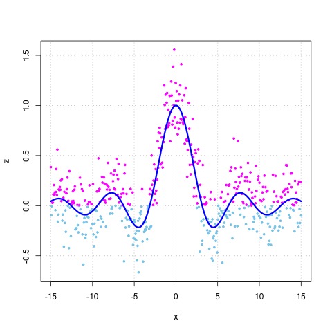
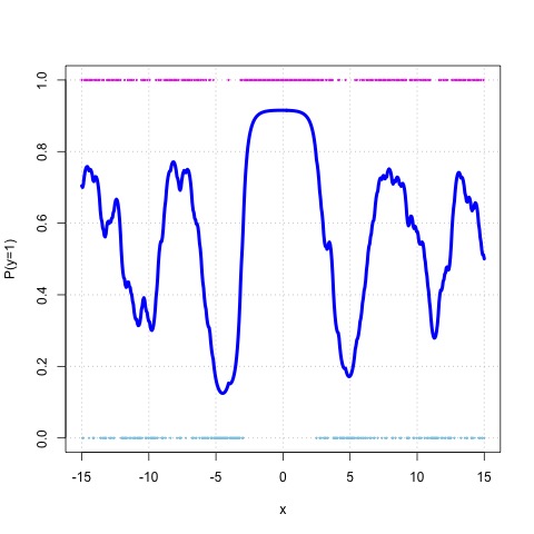
(a)	(b)
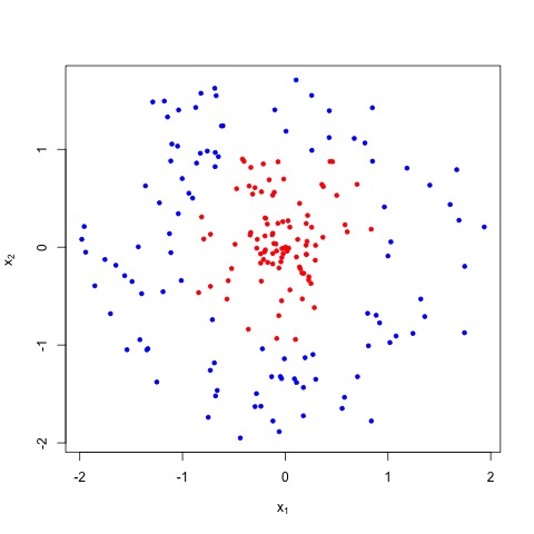
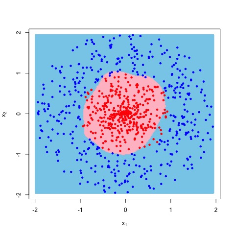
(c)	(d)

Figure 1: Figures (a) and (b) show the simulated data and estimated latent sinc function for Example (4.1). Figures (c) and (d) display the simulated data and estimated circular decision boundary for Example (4.2).

Example 4.2.

Circular Classification
In this example, we consider the circular classification problem. We simulate the data using the following strategy: we generate $x_{1}$ and $x_{2}$ by using the transformation $x_{1}=r\sin(\theta)$ and $x_{2}=r\cos(\theta)$, where $r\sim\text{Uniform}(0,2)$ and $\theta\sim\text{Uniform}(-\pi,\pi)$. We classify the points as red if $r<1$ or blue if $r\geq 1$. We simulate 1000 data points, out of which we keep 200 for training and 800 for testing. We then estimate $\mathbb{P}(y=1)=p$ as a function of $(x_{1},x_{2})$ using GP classification with the Jacobi solution for $\eta$. In Figure (1c), we showcase the 200 points used for training GP classification with the Jacobi solution. Figure (1d) depicts the 800 test points, and the shaded blue and pink regions illustrate the decision boundary estimated from the 200 training points. The out-of-sample accuracy reaches $96.75\%$.

Figure (1 c) displays the 200 points utilized for training GP classification with the Jacobi solution. In Figure (1 d), we present the 800 test points, with the shaded blue and pink regions representing the decision boundary estimated based on the 200 training points. The out-of-sample accuracy achieves $96.75\%.$ The standard statistical models, such as logistic regression or discriminant analysis, generally fail to address the circular classification problem unless we provide many engineered features. The book by Goodfellow et al. (2016), page 4, motivated the idea of "deep learning," while criticizing the standard statistical machine learning models. Here, we demonstrate that the traditional Gaussian process model can address circular classification without any difficulties.

4.2 Multi-Class Classification with Distributed Multinomial Regression

We consider the distributed multinomial regression as presented in Equations (3.7,3.9,3.10). That is

$$P({\mbox{\boldmath$Y$}}_{i}={\mbox{\boldmath$y$}}_{i}) = Multinomial({\mbox{\boldmath$y$}}_{i};m_{i},{\mbox{\boldmath$p$}}_{i})\times Poisson(m_{i};\Lambda_{i}),$$ (4.3)

where ${\mbox{\boldmath$p$}}_{i}=(p_{i1},p_{i2},\cdots,p_{id})$, $p_{ik}=\frac{e^{\eta_{ik}}}{\Lambda_{i}}$, $\Lambda_{i}=\sum_{k=1}^{K}e^{\eta_{ik}}$, and $\eta_{ik}={\mbox{\boldmath$x$}}_{i}^{T}\mbox{\boldmath$\beta$}_{k}$. As $Y_{ik}$ has been drawn independently from the $Poisson(\lambda_{ik})$, where $\lambda_{ik}=e^{\eta_{ik}}=e^{{\mbox{\boldmath$x$}}_{ik}^{T}\mbox{\boldmath$\beta$}_{k}}$ is the Poisson with intensity. In matrix notation we can express it as

$${\mbox{\boldmath$Y$}}_{k}\sim Poisson(\mbox{\boldmath$\lambda$}_{k}),\leavevmode\nobreak\ \leavevmode\nobreak\ \leavevmode\nobreak\ k=1,2,\cdots,K,$$

where

$$\log(\mbox{\boldmath$\lambda$}_{k})=\mbox{\boldmath$\eta$}_{k}.$$

There are $k$ equations which can be presented as,

$$\mbox{\boldmath$\eta$}={\mbox{\boldmath$X$}}\mbox{\boldmath$\beta$}+{\mbox{\boldmath$W$}}+\mbox{\boldmath$\varepsilon$},$$

where $\eta$ is $n\times k$ latent response variables, $X$ is $n\times p$ feature matrix, $\beta$ is $p\times k$ regression coefficient matrixm $W$ is the $n\times k$ random effect matrix and $\epsilon$ is $n\times k$ residual matrix. We assume $W$ is realisation from $K$-variate Gaussian process and $\varepsilon$ is realisation from $K$ variate Normal distribution with identity matrix, i.e.,

$$\varepsilon \sim N(0,{\mbox{\boldmath$I$}}_{k}),$$

$$W \sim GP(\bf{0},\Sigma).$$

The $\eta$ can be estimated as

$$\hat{\mbox{\boldmath$\eta$}}=\ln\bigg{(}\frac{{\mbox{\boldmath$Y$}}+a}{1+b}\bigg{)},$$

the Jacobi estimator for predictive mean for test point ${\mbox{\boldmath$X$}}_{0}$ would be

$$\hat{\mbox{\boldmath$\eta$}}_{0}={\mbox{\boldmath$X$}}_{0}\hat{\mbox{\boldmath$\beta$}}+\mbox{\boldmath$\Sigma$}({\mbox{\boldmath$X$}}_{0},{\mbox{\boldmath$X$}})\Big{[}\mbox{\boldmath$\Sigma$}({\mbox{\boldmath$X$}},{\mbox{\boldmath$X$}})+\sigma^{2}{\mbox{\boldmath$I$}}_{n}\Big{]}^{-1}(\hat{\mbox{\boldmath$\eta$}}-{\mbox{\boldmath$X$}}\hat{\mbox{\boldmath$\beta$}}).$$

Note that once we estimate the $\eta$, the prediction would go the same way using the multinomial probability and predicting the class for maximum probability.

5 Simulation Study

Here, we present four experiments. The aim of this simulation study is to assess the performance of the Jacobi prior approach in comparison to other widely-used methods, such as MLE, Lasso, Ridge, Elastic Net, and Horseshoe prior, for logistic regression, Poisson regression, and distributed multinomial logistic regression. All the codes for all four experiments are available here: https://github.com/sourish-cmi/Jacobi-Prior/.

Experiment 5.1.

Binary Classification with Logistic Regression
We simulate the data from the true model

$$y \sim Bernoulli({\mbox{\boldmath$p$}})$$

$$p = \frac{\exp\{{\mbox{\boldmath$x$}}^{T}\mbox{\boldmath$\beta$}\}}{1+\exp\{{\mbox{\boldmath$x$}}^{T}\mbox{\boldmath$\beta$}\}}$$ (5.1)

We conducted a simulation study with 500 datasets, each comprising a sample size of $n$ with eight predictors. The true parameter vector $\beta$ was set to $(3,1.5,0,0,2,0,0,0)^{T}$ and $\sigma$ was set to $3$. The pairwise correlation between predictors ${\mbox{\boldmath$x$}}_{i}$ and ${\mbox{\boldmath$x$}}_{j}$ was defined as $\rho(i,j)=0.5^{|i-j|}$ for $i,j=1,2,\cdots,p(=8)$. The design matrix ${\mbox{\boldmath$X$}}_{n\times p}$ was generated from $\mathcal{N}(\mbox{\boldmath$\mu$},\mbox{\boldmath$\Sigma$})$, where $\mbox{\boldmath$\Sigma$}=\sigma\rho^{|i-j|}$. Given ${\mbox{\boldmath$x$}}_{i}$ for $i=1,2,\cdots,n$ the response variable $y_{i}$ was generated from Equation (5.1). We generated a total of $M(=500)$ datasets, denoted as $\mathcal{D}^{s}=\{{\mbox{\boldmath$y$}}^{s},{\mbox{\boldmath$X$}}^{s}_{n\times p}\}$ for $s=1,2,\cdots,M(=500)$ with the true parameter $\mbox{\boldmath$\beta$}=\mbox{\boldmath$\beta$}_{0}$. For a sample size of $n=100$, the estimates of $\beta$ from the $s^{th}$ dataset, $\mathcal{D}^{s}$ were denoted as $\hat{\mbox{\boldmath$\beta$}}^{s}$. The predicted response $\hat{{\mbox{\boldmath$p$}}}^{s}$ was calculated as $\mathbb{E}({\mbox{\boldmath$y$}}^{s})=\hat{{\mbox{\boldmath$p$}}}^{s}=\frac{\exp\{{\mbox{\boldmath$x$}}^{T}\hat{\mbox{\boldmath$\beta$}}^{s}\}}{1+\exp\{{\mbox{\boldmath$x$}}^{T}\hat{\mbox{\boldmath$\beta$}}^{s}\}}$. The root mean square error (RMSE) for the $s^{th}$ data set was computed as

$$RMSE^{s}=\sqrt{\frac{1}{n}({\mbox{\boldmath$y$}}^{s}-\hat{{\mbox{\boldmath$p$}}}^{s})^{T}({\mbox{\boldmath$y$}}^{s}-\hat{{\mbox{\boldmath$p$}}}^{s})}.$$

We implemented the Jacobi prior using the solution presented in Equation (3.3), with $a=b=1/2$ and $m=1$. We implemented the Lasso, Ridge and Elastic Net, using the $5$-fold cross validation method using the glmnet package in R. We implemented the horseshoe prior using bayesreg package in R. It uses 5000 MCMC samples to estimates the $\beta$. The findings are displayed in Table (1). It is worth highlighting that the Jacobi prior demonstrates superior performance compared to other methods, showcasing enhanced predictive accuracy and better efficient time complexity. All codes of this experiment is being provided here https://github.com/sourish-cmi/Jacobi-Prior/.

	RMSE($y$)	SE	RMSE($\beta$)	SE	Time	SE	Multiples
MLE	0.69	0.01	1.97	0.28	1003.98	0.02	18.63
Ridge	0.61	0.00	0.97	0.00	13162.61	0.02	244.28
Lasso	0.66	0.00	0.58	0.01	18862.01	0.38	350.06
Elsatic Net	0.66	0.00	0.62	0.01	15560.39	0.08	288.78
Horseshoe	0.68	0.01	0.62	0.03	2763397.57	2.93	51285.53
Jacobi Prior	0.54	0.00	1.23	0.00	53.88	0.00	1.00

Table 1: For the simulation Experiment (5.1), based on 500 replications, the out sample median RMSE of $y$, median RMSE of $\beta$ and median time (in microseconds) taken by six methods are presented.

Remark 5.1.

In the first column of the Table (1), we present the out of the sample median RMSE of prediction for different methods calculated over 500 simulated datasets, indicating the predictive performance of Logistic Regression. A lower RMSE indicates better predictive accuracy. The number in second columns are the corresponding standard errors of median RMSE, estimates by using the bootstrap with $B=1000$ resampling on the 500 RMSEs. The third column presents median RMSE of the estimates of the $\beta$. The fifth column shows the median time taken by each methodology in microseconds across the 500 datasets. It is noteworthy that the Jacobi prior outperforms other methods, exhibiting both superior predictive accuracy and more efficient time complexity. In the last column, we provide the time taken by different methods relative to the Jacobi prior solution. The Jacobi prior is over 200 times faster than any method using glmnet and approximately 18 times faster than Fisher’s scoring-based MLE.

Remark 5.2.

In the current landscape of cloud computing, time is often equated with monetary value, as cloud services are billed according to usage duration. The Jacobi prior stands out for providing accurate predictions and doing so much faster. This increased efficiency not only saves money for cloud users but also helps organizations reduce their environmental impact. Reducing operational time and energy use supports ESG goals, offering both cost savings and environmental benefits.

Experiment 5.2.

Statistical Consistency of Jacobi Estimator for Logistic Regression
Here we consider the setup of Experiment (5.1). In this experiment, we want to check if the Jacobi estimator of $\beta$ for the logistic regression model presented in Equations (5.1) is statistically consistent. We considered the increasing sample size from $n=200$ to $5000$. For each sample size, we ran the experiment exactly the same as Experiment (5.1). When we consider $a=b=1/2$, for all choices of $n$, we calculated the RMSE of $\beta$ and plotted the results in Figure (2a), which shows that the Jacobi estimator’s RMSE is constant. It implies the Jacobi estimator is inconsistent when $a=b=1/2$, i.e., when $a$ and $b$ are constant. Next we consider the Jacobi prior when $a=b=1/n$; calculated the corresponding RMSE of $\beta$ for different choices of $n$ and plotted the results in Figure (2b). When we choose $a=b=\frac{1}{n}$, the RMSE of Jacobi estimator decrease with increasing $n$, like MLE. It implies that both bias and variance tend to zero with increasing sample size. Hence, the experiment indicates that the Jacobi estimator is statistically consistent when $a=b=\frac{1}{n}$.

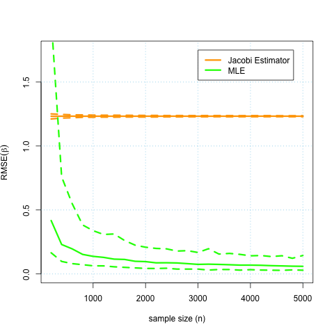
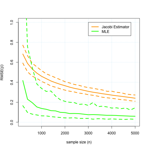
(a)	(b)

Figure 2: Figure presents the RMSE of $\beta$ of Logistic Regression with increasing sample size ($n$), when (a) $a=b=1/2$; and (b) $a=b=1/n$

Experiment 5.3.

Poisson Regression for Count Data
We simulate the data from the true model

$$y \sim Poisson(\lambda)$$

$$\lambda = \exp\{{\mbox{\boldmath$x$}}^{T}\mbox{\boldmath$\beta$}\}.$$

We performed a simulation study with 500 datasets, each having a sample size of $n$ and eight predictors. The true parameter vector $\beta$ was set to $(0.3,0.15,0,0,0.2,0,0,0)^{T}$ and $\sigma$ was set to $1$. The pairwise correlation between predictors ${\mbox{\boldmath$x$}}_{i}$ and ${\mbox{\boldmath$x$}}_{j}$ was setup as in the Example (5.1). For a sample size of $n=100$, the estimates of $\beta$ from the $s^{th}$ dataset, $\mathcal{D}^{s}$ were denoted as $\hat{\mbox{\boldmath$\beta$}}^{s}$. The predicted response $\hat{\lambda}^{s}$ was calculated as $\mathbb{E}({\mbox{\boldmath$y$}}^{s})=\hat{\lambda}^{s}=\exp\{{\mbox{\boldmath$x$}}^{T}\hat{\mbox{\boldmath$\beta$}}^{s}\}$. We implemented the Jacobi prior using the solution presented in Equation (3.5), with $a=b=1$ and $m=1$. We implemented Lasso, Ridge, and Elastic Net using the 5-fold cross-validation method with the glmnet package in R. The findings are displayed in Table (2). It is worth noting that the Jacobi prior demonstrates superior performance compared to other methods, showcasing enhanced predictive accuracy and more efficient time complexity.

Methods	Median RMSE	SD of RMSE	Time	Multiplier
MLE	1.33	0.30	836.97	15.53
Ridge	1.21	0.28	12021.06	223.07
Lasso	1.22	0.28	10387.18	192.77
Elsatic Net	1.21	0.28	10825.39	200.91
Horseshoe	1.21	0.28	3850750.09	71465.56
Jacobi Prior	1.17	0.26	53.88	1.00

Table 2: Median RMSE and Time Complexity of Experiment (5.3)

.

In the first column of Table (2), we present the Median RMSE of different methods calculated over 500 datasets, indicating the predictive performance of Poisson regression. A lower RMSE indicates better predictive accuracy. The second column displays the standard deviation of RMSE across these 500 datasets. The third column shows the median time taken by each methodology in microseconds. Notably, the Jacobi prior outperforms other methods, showcasing both superior predictive accuracy and more efficient time complexity. In the fourth column, we present the time taken by different methods relative to the Jacobi prior solution. The Jacobi prior is more than 150 times faster than any glmnet methods and about 15 times faster than Fisher’s scoring-based MLE.

Experiment 5.4.

K-Class Classification with Distributed Multinomial Logistic Regression
We simulate the data from the model

$$y \sim Multinomial({\mbox{\boldmath$s$}},{\mbox{\boldmath$p$}})$$

$$p \sim (p_{1},p_{2},\cdots,p_{K})$$

$$p_{k} = \frac{\exp\{{\mbox{\boldmath$x$}}^{T}\mbox{\boldmath$\beta$}_{k}\}}{\sum_{k=1}^{K}\exp\{{\mbox{\boldmath$x$}}^{T}\mbox{\boldmath$\beta$}_{k}\}},$$

$$x = \{x_{1},x_{2},\cdots,x_{P}\}.$$

We consider number of class as $K=4$, number of features as $P=3$, sample size $n=50$ and simulated 100 such data sets; where we simulated $\beta$ for each data sets using following strategy,

$$\mbox{\boldmath$\beta$}_{(P+1)\times K} \sim \mathcal{N}(0,1),$$

$$\beta_{j,k} = \begin{cases}\beta_{j,k}&\text{with probability 0.5},\\ 0&\text{with probability 0.5}.\end{cases}$$

where $j=1,2,\cdots,P$, $k=1,2,\cdots,K$. The strategy induces $50\%$ sparsity in the solution space. Once the coefficient matrix $\beta$ is simulated it is treated as true parameter, denoted as $\mbox{\boldmath$\beta$}_{0}$. The predictors $x$ is simulated from uniform(0,1) and response is being $y$ from Multinomial(${\mbox{\boldmath$s$}},{\mbox{\boldmath$p$}}$), where ${\mbox{\boldmath$s$}}\sim Poisson(\lambda=10)$. We applied the Lasso, Ridge, and Elastic Net methods using the 5-fold cross-validation technique, utilizing the glmnet package in R. Similarly, we employed the bayesreg package in R to implement the horseshoe prior. This method involves using 12000 MCMC samples to estimate the $\beta$ and implemented for all 100 datasets.

Methods	Median RMSE	Sd of RMSE	Time	Multiple
Full Multinomial
Regression
Elastic Net	0.72	0.35	62437.53	931.96
Ridge	0.72	0.33	61874.15	923.56
Lasso	0.74	0.36	70528.51	1052.73
Distributed Multinomial
Regression
Elastic Net	0.71	0.38	46859.03	699.43
Ridge	0.74	0.38	55206.06	824.02
Lasso	0.71	0.38	46835.54	699.08
Horseshoe	0.74	0.33	9855186.00	147101.94
Jacobi Prior	0.62	0.32	66.99	1.00

Table 3: Median RMSE and Run-Time Complexity of Experiment (5.4)

In the first column of the Table (3), we report the median RMSE for various methods, calculated across 100 datasets. This serves as an indicator of the predictive efficiency in DMLR regression, where a lower RMSE signifies enhanced predictive accuracy. The second column illustrates the standard deviation of the RMSE over these datasets. The median duration each method, measured in microseconds, is depicted in the third column. Notably, the Jacobi prior demonstrates exceptional performance, excelling in both predictive accuracy and computational efficiency. The fourth column compares the time efficiency of different methods to that of the Jacobi prior. Remarkably, the Jacobi prior is over 600 times quicker than any glmnet method and horseshoe prior.

6 Empirical Study

6.1 Galaxies, Quasars, and Stars: Three Class Classification

In the field of astronomy, the classification of stars, galaxies, and quasars using machine learning is vital for gaining insights into the universe’s diverse components (see Clarke, A. O. et al. (2020)). This classification, based on spectral characteristics, holds significant importance. The dataset under consideration comprises 100,000 space observations collected through the Sloan Digital Sky Survey (SDSS) Abdurro’uf and etal (2022). Each observation is defined by seven distinct features, complemented by an additional class label that designates it as a star, galaxy, or quasar. This dataset is tailored to streamline the classification of stars, galaxies, and quasars, making use of their distinctive spectral properties. The descriptions of the seven features of the SDSS data sets is presented in the Table (4).

	Feature Name	Description
1	alpha	Right Ascension angle (at J2000 epoch)
2	delta	Declination angle (at J2000 epoch)
3	u	Ultraviolet filter in the photometric system
4	g	Green filter in the photometric system
5	r	Red filter in the photometric system
6	i	Near Infrared filter in the photometric system
7	z	Infrared filter in the photometric system

Table 4: Description of the features of the SDSS datasets.

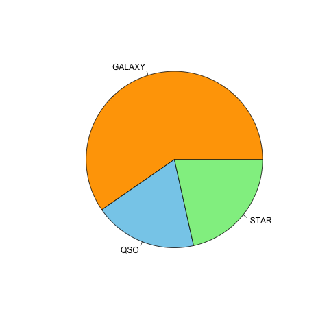
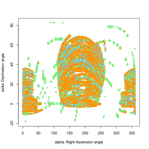
(a)	(b)
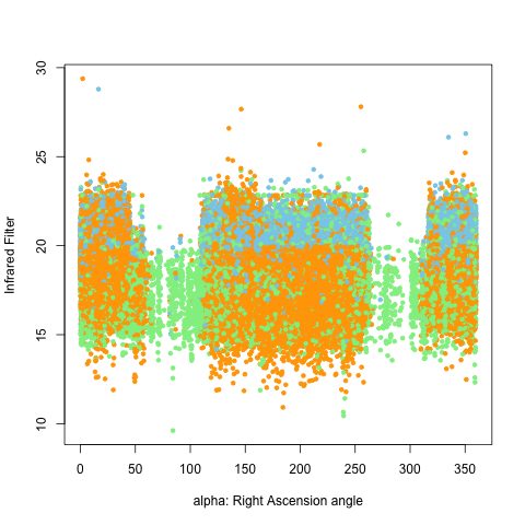
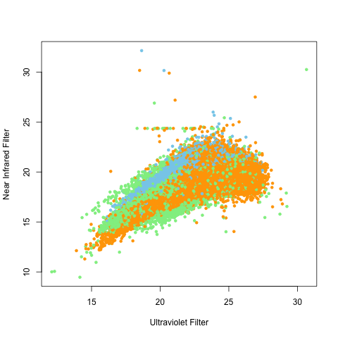
(c)	(d)

Figure 3: A graphical presentation of SDSS data to visualize different features and the type of astronomical object.

The dataset is split into train and test sets. Seventy percent of the data is randomly selected for training, while the remaining ($30\%$) is kept for testing. Exploratory data analysis (EDA) is conducted using the training dataset, and a few graphs are presented in Figure (3). Detailed EDA can be found at the following GitHub link: https://github.com/sourish-cmi/Jacobi-Prior/. The pie chart in Figure (3a) illustrates the distribution of galaxies, quasars, or stars in the training dataset. Figure (3b) shows the scatter plot between alpha (i.e., right ascension angle) and delta (i.e., declination angle), indicating a highly non-linear relationship between the variables. Figure (3c) presents the scatter plot between alpha and infrared filter. The graph indicates that when the right ascension angle (i.e., alpha) is between 60-120 or 260-320, the chance that the object is a star is very high. Similarly, Figure (3d) presents the scatter plot between ultraviolet filter and near-infrared filter, indicating highly non-linear relationships. It is evident that stars are significantly different from galaxies and quasars.

We consider the task of 3-class classification, where the classes are namely stars, galaxies, and quasars. We implement the Distributed Multinomial Regression with Poisson model, incorporating Ridge, Lasso, and Elastic Net regularization, along with the Jacobi Prior. In addition, we also implement the regular Multinomial Regression model using the glmnet package in R. In Table (5), we present the out-of-sample accuracy and run-time (in seconds) of different methods. The out-of-sample accuracy of the Jacobi prior and the Lasso penalty are almost the same. However, in terms of run-time, the Jacobi prior is nearly 500 times faster than the Lasso penalty.

Methods	Accuracy	Time	Multiple
Distributed Multinomial Regression
with Jacobi Prior	73.05	0.69	1.00
with Ridge Penalty	61.67	13.06	18.89
with Lasso Penalty	72.94	348.58	504.28
with Elastic Net	72.71	376.63	544.86
Full Multinomial Regression
with Ridge Penalty	62.83	65.21	94.33
with Lasso Penalty	70.97	575.74	832.93
with Elastic Net	72.48	641.84	928.53

Table 5: Out-sample accuracy and runtime complexity comparison of different methods for Multinomial regression on the SDSS star classification dataset.

6.2 Loan Approved or Denied

In this study, we employed a rich dataset obtained from the U.S. Small Business Administration (SBA) (The U.S. Small Business Administration, 2020; Li et al., 2018), comprising 899,164 samples. This dataset captures a diverse range of scenarios, including notable success stories of startups benefiting from SBA loan guarantees, as well as instances of small businesses or startups facing defaults on their SBA-guaranteed loans. Our primary objective in analyzing this dataset is to predict the probability of default. Upon reviewing the dataset, the central question emerges: should a loan be granted to a specific small business? This decision hinges on a thorough evaluation of various factors, necessitating a nuanced exploration of the loan approval or denial criteria. In this study we considered five features, described in Table (6).

	Feature Name	Description
1	New	1 = Existing business, 2 = New business
2	RealEstate	If backed by real estate
3	DisbursementGross	Amount disbursed
4	Term	Loan term in months
5	NoEmp	Number of business employees

Table 6: Description of the features of the US SBA Loan Approval Dataset

We implemented simple logistic regression using the glm function in R. Additionally, we implemented regularization methods such as Lasso, Ridge, and Elastic Net using the glmenet package in R. We also implemented the Jacobi prior with four different techniques. To choose the hyperparameters $a$ and $b$, we considered $a=b=0.5$ (Jeffrey’s prior for $p$); $a=6/10$, and $b=4/10$, an ad-hoc choice. Furthermore, we implemented a stochastic search for $a$ and $b$, and finally, we employed a Bayesian optimization method to estimate $a$ and $b$. The prediction in the loan default problem entails two types of errors with different consequences. Along with the accuracy of the prediction, we also estimate the utility of the prediction. We define the utility of the prediction for a single loan in the following Table (7). We calculate the utility of all the loans and add them up.

	Denie	Approve
Default	$V*0.1$	$-V*0.7$
No Default	$-V*0.1$	$V*0.5$

Table 7: Utility of the prediction. The $V$ is the Gross Disbursement amount.

Out-sample accuracy, utility of prediction and runtime complexity comparison of different methods are presented in Table (8). The outcomes from the dataset on loan approval or denial by the USA Small Business Association reveal that employing Jacobi Prior with Stochastic Optimization leads to higher accuracy, enhanced utility, and an average speed improvement of more than 200 times compared to conventional solutions such as Lasso, Ridge, and Elastic Net.

Method	Accuracy	Utility	Time	Multiples
MLE	82.74	19.31	1.49	16.56
Lasso	82.70	19.32	20.06	222.88
Ridge	82.72	19.46	38.73	430.33
Elastic Net	82.68	19.32	21.85	242.78
Jacobi Prior: a=b=0.5	82.35	19.16	0.09	1.00
Jacobi Prior: a=6/10, b=4/10	83.41	19.31	0.09	1.00
Jacobi Prior: Stochastic Optim	83.04	19.82	0.11	1.22
Jacobi Prior: Bayes Optim	83.19	19.84	19.75	219.44

Table 8: Out-sample accuracy, utility of prediction and runtime complexity comparison of different methods for Logistic regression on the US SAB loan dataset.

7 Concluding Remarks

In conclusion, this study introduces the Jacobi prior as an alternative Bayesian method aimed at mitigating the computational challenges inherent in traditional techniques. Through comprehensive experimentation, we have demonstrated the superior performance of the Jacobi prior over well-established methods such as Lasso, Ridge, Elastic Net, and MCMC-based Horse-Shoe Prior methods, particularly in terms of predictive accuracy. Moreover, our findings indicate that the Jacobi prior exhibits remarkable efficiency, surpassing these methods by more than 100 times in terms of runtime while maintaining comparable predictive accuracy.

The versatility of the Jacobi prior is underscored by its successful implementation across various models, including Generalised Linear Models, Gaussian process regression, and classification. Its capability to handle partitioned data distributed over different servers across continents further enhances its applicability in diverse and distributed computing environments.

Notably, the superior runtime performance of the Jacobi prior aligns with the growing imperative for organizations to minimize their carbon footprint and uphold long-term compliance with environmental, social, and governance (ESG) standards. By offering substantial computational efficiency without sacrificing predictive accuracy, the Jacobi prior presents a promising solution for organizations navigating these sustainability challenges.

Our comprehensive simulation and empirical studies validate the effectiveness of the Jacobi prior across different contexts, including credit risk estimation and classification problems in astronomy. The availability of codes and datasets in our GitHub repository facilitates reproducibility and further exploration of our findings, contributing to the advancement of Bayesian methodology in data analysis.

In summary, the Jacobi prior emerges as a robust and efficient tool for Bayesian inference, offering a compelling alternative to traditional methods and paving the way for enhanced predictive modeling across various domains.

References

- Abdurro’uf and etal (2022) Abdurro’uf and etal (2022). The seventeenth data release of the sloan digital sky surveys: Complete release of manga, mastar, and apogee-2 data. The Astrophysical Journal Supplement Series 259(2), 35.
- Bonnier and Bosch (2023) Bonnier, T. and B. Bosch (2023). Towards safe machine learning lifecycles with esg model cards. In J. Guiochet, S. Tonetta, E. Schoitsch, M. Roy, and F. Bitsch (Eds.), Computer Safety, Reliability, and Security. SAFECOMP 2023 Workshops, Cham, pp. 369–381. Springer Nature Switzerland.
- Carvalho et al. (2010) Carvalho, C. M., N. G. Polson, and J. G. Scott (2010). The horseshoe estimator for sparse signals. Biometrika 97(2), 465–480.
- Clarke, A. O. et al. (2020) Clarke, A. O., Scaife, A. M. M., Greenhalgh, R., and Griguta, V. (2020). Identifying galaxies, quasars, and stars with machine learning: A new catalogue of classifications for 111 million sdss sources without spectra. A&A 639, A84.
- Das (2008) Das, S. (2008). Generalized linear models and beyond: An innovative approach from Bayesian perspective. Ph. D. thesis, University of Connecticut, Storrs.
- Das and Dey (2006) Das, S. and D. K. Dey (2006). On bayesian analysis of generalized linear models using the jacobian technique. The American Statistician 60(3), 264–268.
- Das and Dey (2010) Das, S. and D. K. Dey (2010). On bayesian inference for generalized multivariate gamma distribution. Statistics & Probability Letters 80(19), 1492–1499.
- Das et al. (2018) Das, S., S. Roy, and R. Sambasivan (2018). Fast gaussian process regression for big data. Big Data Research 14, 12–26.
- Goodfellow et al. (2016) Goodfellow, I., Y. Bengio, and A. Courville (2016). Deep Learning. MIT Press. http://www.deeplearningbook.org.
- Hastie et al. (2009) Hastie, T., R. Tibshirani, and J. Friedman (2009, February). The Elements of Statistical Learning: Data Mining, Inference, and Prediction (2 ed.). Springer.
- Li et al. (2018) Li, M., A. Mickel, and S. Taylor (2018). "should this loan be approved or denied?": A large dataset with class assignment guidelines. Journal of Statistics Education 26(1), 55–66.
- Park and Casella (2008) Park, T. and G. Casella (2008). The bayesian lasso. Journal of the American Statistical Association 103(482), 681–686.
- Sandhu (2022) Sandhu, A. K. (2022). Big data with cloud computing: Discussions and challenges. Big Data Mining and Analytics 5(1), 32–40.
- Taddy (2015) Taddy, M. (2015). Distributed multinomial regression. The Annals of Applied Statistics 9(3), 1394 – 1414.
- The U.S. Small Business Administration (2020) The U.S. Small Business Administration (2020). Should this loan be approved or denied? data retrieved from Kaggle, https://www.kaggle.com/datasets/mirbektoktogaraev/should-this-loan-be-approved-or-denied.
- Tibshirani (1996) Tibshirani, R. (1996). Regression shrinkage and selection via the lasso. Journal of the Royal Statistical Society. Series B (Methodological) 58(1), 267–288.
- Zou and Hastie (2005) Zou, H. and T. Hastie (2005). Regularization and variable selection via the elastic net. Journal of the Royal Statistical Society. Series B (Statistical Methodology) 67(2), 301–320.