Modern tools for computing neutron star properties
Abstract
Astronomical observations place increasingly tighter and more diverse constraints on the properties of neutron stars (NS). Examples include observations of radio or gamma-ray pulsars, accreting neutron stars and x-ray bursts, magnetar giant flares, and recently, the gravitational waves (GW) from coalescing binary neutron stars. Computing NS properties for a given EOS, such as mass, radius, moment of inertia, tidal deformability, and innermost stable circular orbits (ISCO), is therefore an important task. This task is unnecessarily difficult because relevant formulas are scattered throughout the literature and publicly available software tools are far from being complete and easy to use. Further, naive implementations are unreliable in numerical corner cases, most notably when using equations of state (EOS) with phase transitions. To improve the situation, we provide a public library for computing NS properties and handling of EOS data. Further, we include a collection of EOS based on existing nuclear physics models together with precomputed sequences of NS models. All methods are accessible via a Python interface. This article collects all relevant equations and numerical methods in full detail, including a novel formulation for the tidal deformability equations suitable for use with phase transitions. As a sidenote to the topic of ISCOs, we discuss the stability of non-interacting dark matter particle circular orbits inside NSs. Finally, we present some simple applications relevant for parameter estimation studies of GW data. For example, we explore the validity of universal relations, and discuss the appearance of multiple stable branches for parametrized EOS.
pacs:
04.25.dk, 04.30.Db, 04.40.Dg, 97.60.Jd,I Introduction
Neutron stars (NS) are among the most interesting astrophysical objects, as their description requires both general relativity and nuclear physics. The latter comes into play via the equation of state (EOS) of matter up to densities exceeding nuclear saturation density. The EOS is assumed to be universal, i.e., not dependent on the star’s origin. NSs are distinguished individuals with different surface temperature, magnetic field strengths and topologies, rotation rates, and propensity for glitches or radiation outbursts. However, they can be described by a few scalar properties well enough for many astrophysical applications. The most basic NS features are captured by the simple case of slowly rotating, non-magnetized stars. Such models are completely determined by the central density and the EOS. The purpose of this paper and the provided software is to enable readers to compute those models with ease.
The most important NS properties are the following. First and foremost, the gravitational mass, which completely determines the metric outside the NS. There is also a “baryonic mass”, which expresses the baryon number in units of mass, and which is important as a conserved quantity, e.g., in the context of neutron star mergers. The difference between baryonic and gravitational mass defines the binding energy. The NS size is usually expressed as the proper circumferential radius, which also determines the surface area. Another important property is the compactness, defined as gravitational mass over proper circumferential radius. It directly determines the surface redshift, and is strongly correlated with other properties such as oscillation frequencies, moment of inertia, or tidal deformability. The moment of inertia is obviously relevant for questions related to spin-down or glitches. It also determines the lowest order rotational corrections to the metric in comparison to the nonrotating case. The tidal deformability of a NS is the proportionality factor between external tidal fields and the induced quadrupole moment. It is very important for the late inspiral phase of BNS mergers as it determines the main corrections of the orbital dynamics compared to the binary black hole case, and thus the observable gravitational wave (GW) signal.
The equations governing mass and radius of nonrotating neutron stars (NS) are known since the early work by Tolman (1939); Oppenheimer and Volkoff (1939). This also established that the NS mass is bounded, and that the maximum mass depends on the EOS. Not all solutions for static NS are stable against radial perturbations. The single parameter sequence of NS consists of one or more stable and unstable branches, which depends on the EOS. Criteria for the stability have been collected by Bardeen et al. (1966). The equations for the moment of inertia were derived by Hartle (1967) for slowly rotating NS. More recently, equations that govern the tidal deformability have been derived in Hinderer (2008, 2009); Flanagan and Hinderer (2008); Hinderer et al. (2010). The computation of the above properties requires the solution of an ordinary differential equation system (ODE) with singular boundary conditions.
One complication is given by the possibility of phase transitions in the EOS, which can lead to discontinuities in the energy density as function of pressure. We note that phase transitions do not necessarily lead to discontinuities. Those which do are the problematic ones in the context of this work, and we will use the terms synonymously in the following. Although a true discontinuity can be treated analytically for the tidal deformability ODE Postnikov et al. (2010); Takátsy and Kovács (2020), such treatment is infeasible for the more typical case of EOS that merely exhibit very sharp features. That case is also problematic for direct numerical solution.
Measurements of NS properties can help to constrain the equation of state (EOS) of neutron star matter. There are different avenues towards this goal. Any measurement of a NS mass provides a lower bound for the maximum NS mass. Another avenue is the measurement of mass-radius relations by electromagnetic observations (see, e.g., Özel et al. (2010); Özel and Freire (2016); Özel (2006)). The moment of inertia can also serve to constrain the EOS and might be measured, e.g., via observation of double pulsar systems Raithel et al. (2016). Another possibility is the measurement of mass and tidal deformability using observations of gravitational waves from BNS coalescence, such as the famous event GW170817 Abbott et al. (2017a, 2019a, 2019b, b); Aasi et al. (2015); Acernese et al. (2015). Further, the stability of a BNS merger remnant is related to the maximum NS mass. If electromagnetic counterparts in a BNS multimessenger observation carry information on the fate of the remnant, it can be used to constrain the EOS. This was already done (under additional assumptions) using the short gamma ray burst associated with GW170817 Abbott et al. (2017c).
Despite the astrophysical importance of computing NS properties, the available software infrastructure is very limited. Although there exists a plethora of solvers for the basic NS structure, these codes are severely lacking with regard to some of the following aspects: a) public availability b) ease of installation c) documentation d) dependence on free open source software only e) reliability, also in corner cases f) error estimates g) code quality h) usability from within other codes i) completeness of NS properties and j) EOS handling.
One purely technical hurdle is the lack of a standardized exchange format for generic EOS. One notable file format for tabulated nuclear physics EOS is developed by the CompOSE project Typel et al. (2018). It is well-documented and complete in the sense that all required metadata is contained. However, this standard does not allow popular analytic EOS models, leaves the interpolation method unspecified, and lacks an easy to use interface for reading and evaluating an EOS from within other code.
The aim of our work is to address all of the above issues. Recently, we provided tools for computing NS properties as part of the library RePrimAnd, which was developed to support general relativistic magnetohydrodynamics simulations Kastaun et al. (2021). It also provides an elaborate framework for handling of EOS. The library is publicly available and documented Kastaun (2024a). It can be used from within C++ or Python.
This article collects everything required for computing NS properties in the RePrimAnd library, such as basic notation and definitions, all equations needed for computing NS structure, and a discussion how to avoid numerical pitfalls. We convert formulas scattered across the literature into a coherent notation and point out details that are usually not discussed but important for actual computations. Further, we reformulate some equations to facilitate numerical solution. Most notably, we provide a formulation of the differential equations for tidal deformability that is robust when the EOS exhibits phase transitions, and we correct a faulty approximation for the limit of low compactness.
We also perform extensive tests of the accuracy, which leads to a model for the error bounds. This model is incorporated in the library, allowing to directly specify the desired accuracy. A related practical problem regards the impact of approximated EOS representations that use interpolation and low-density extrapolation. We will provide some guidance regarding requirements for tabulated EOS.
Finally, we present some simple results obtained with the new library, which might be useful for gravitational wave (GW) and multi-messenger astronomy. Firstly, we collect NS properties for a number of nuclear physics EOS available in the literature, such as tidal deformability and moment of inertia. Next, we study the reliability of empirical relations between NS compactness and tidal deformability that allegedly depend only weakly on the EOS, by performing numerical searches for EOS causing larger deviations. The finding are relevant for studies that combine constraints of mass-radius and mass-tidal deformability relations, e.g., using NICER and GW data. We also point out how splitting of stable branches complicates parameter estimation with parametrized EOS for BNS GW detections. Last but not least, we provide a small collection of ready-to-use EOS files representing existing nuclear physics EOS models.
II Formulation
In the following we collect all equations needed for computing the properties of nonrotating NS. Most are well known but scattered throughout the literature and use different notation and conventions. We recast some expressions into the variants that are employed in the RePrimAnd library, and which are advantageous for numerical solution. The main novelty, described in Sec. II.4, is our new formulation of the ODE that governs tidal deformability, which is applicable also to EOS with phase transitions.
II.1 Conventions
We use geometric units throughout this work unless noted otherwise, that is, units in with . This leaves open one degree of freedom, which can be fixed by choosing a mass unit. Denoting time, length, and mass units by , respectively, the unit system is given by
| (1) |
We stress that when computing NS properties using equations assuming geometric units, the gravitational constant is implicitly given by the geometric unit system. Comparing results obtained in different geometric unit systems is not just a matter of converting back to SI units, unless both use the same value of . In contrast, the choice of the mass unit is irrelevant because, unlike the constant , it is not a physical constant that would appear in the full equations stated in arbitrary units. Often, geometric unit systems are specified by the condition . Without providing the precise values assumed for and , it is impossible to compare results to a precision better than around since both constants are not known very accurately (although their product is). For the NS solutions in this work, we use values of exactly and (from Zyla et al. (2020)).
We assume that NS matter in GR can be described by the stress-energy tensor of a perfect fluid, given by
| (2) |
Above, is the 4-velocity of the fluid, is the total energy density in the restframe of the matter, and is the pressure. This means that we make the approximation of isotropic pressure, and exclude any shear-stresses. For a discussion of NS structure with anisotropic pressure, we refer to Pretel et al. (2023). We note that realistic NS can have minor shear stresses within the crust. This is irrelevant when computing spherical equilibrium models under the assumption of zero shear deformation, and it is commonly neglected when computing the tidal deformability.
We denote the baryon number density in the fluid restframe by . Introducing a mass constant , one can define a “baryonic mass density” (or mass density for short) . The constant is arbitrary and usually chosen around the neutron mass, while the exact value varies between different sources. When comparing baryonic mass density between different sources, this should be taken into account. In the RePrimAnd framework, the convention is .
Further, we will use the specific internal energy and relativistic enthalpy defined by
| (3) | ||||
| (4) |
Note that the definitions of depend on the choice of , such that and differ by a global factor between different choices. The specific internal energy also differs by an offset, not just a factor. In particular, for does not imply that approaches zero, nor that it is positive. The zero-density limit depends on the choice of . The conditions hold independently of this choice, assuming only that .
II.2 Equation of State
In general, NS matter has three degrees of freedom, usually parametrized in terms of baryon number density , temperature , and electron fraction (one usually assumes macroscopic charge neutrality since astrophysical objects are assumed to carry negligible net charge, and NS matter is assumed to be highly conductive). The variables and are equivalent to the thermodynamic state variables (volume) and particle numbers for protons and neutrons.
The behavior of matter is completely described by a single thermodynamic potential, meaning a scalar function of a particular set of state variables. There are different but completely equivalent thermodynamic potentials, each based on a different set of state variables. When using state variables , the corresponding potential is the Helmholtz free energy .
Given a thermodynamic potential and its canonical state variables, one can derive all other quantities. Such derived relations are collectively referred to as equation of state (EOS). For the Helmholtz free energy, pressure and entropy are given by the partial derivatives and , respectively, and the internal energy is given by . We can parametrize the EOS as functions , , and .
For most applications, only the EOS is needed in some form, but not the underlying thermodynamic potential. In fact, nuclear physics models are often distributed as tables sampling the EOS functions. We note that this makes it more difficult to interpolate such tables in a consistent manner. There are also some toy models where the EOS is directly prescribed as analytic expressions.
It should be noted that one cannot chose the various EOS functions independently. The existence of a thermodynamic potential implies thermodynamic consistency constraints. For example, . If those constraints are violated, an EOS is physically invalid. Results based on such inconsistent EOS are not just wrong, but ambiguous, since there are different ways to express the same quantity which cease to yield identical results.
In this work, we are concerned only with scenarios where pressure and energy density can be expressed as functions and of the mass density alone. This is called a barotropic EOS. Physically, employing a barotropic EOS means that two of the matter degrees of freedom are restricted somehow. The most relevant example for our aims is to model cold neutron stars, where thermal effects can be neglected and one can set for all practical purposes. Further, we want to model equilibrium models. For those, the electron fraction becomes a function of density because weak processes drive the matter towards -equilibrium.
For perturbed NS, -equilibrium is maintained if the perturbation timescale is much longer than the intrinsic timescales of weak processes. This is the case for tidal deformations in the limit of large separation. We note that for the timescales accessible to ground-based gravitational wave detectors, approximating deformations as static might be insufficient in any case. For further discussion of dynamical tidal effects see, e.g., Dietrich and Hinderer (2017). Here, we only consider static deformations.
In this work, we assume that pressure cannot be negative, and we exclude exotic types of matter, assuming that and . We further exclude any contributions to energy or pressure unrelated to baryonic matter, such as dark matter clouds or radiation fields outside a NS. Thus, we assume .
An important subset of barotropic EOS is given by the isentropic barotropic EOS, which are defined by a constant specific entropy. A NS model following such an EOS will continue to do so when perturbed adiabatically, i.e., such that and hence . For barotropic EOS, this condition implies that
| (5) |
Our main use case are cold NSs, which indeed follow an isentropic barotropic EOS. One can construct other examples of NS with isentropic barotropic EOS by making the artificial assumption of a radial temperature profile such that the specific entropy remains constant. A counter-example that cannot be modeled that way is a hot NS with constant temperature.
How matter reacts to small perturbations can be expressed by the adiabatic speed of sound, which for an isentropic barotropic EOS is given by the derivative
| (6) |
On physical grounds, we rigorously demand that any EOS satisfies
| (7) |
The condition is required for stability of matter, otherwise perturbations would be exponentially growing instead of propagating as sound waves. This condition sometimes gets violated when stitching together EOS computed for different density regimes, or when interpolating coarsely sampled EOS using ill-suited interpolation methods that produce overshoots.
The causality condition is required for any physically valid model. Already on the mathematical level, the equations that govern relativistic hydrodynamics break down if there are superluminal characteristic speeds. Note that the equations describing the static solutions discussed here do admit mathematically valid solutions also for the case with superluminal soundspeeds. However, we do not consider such solutions since they are not valid in the wider context of the general relativistic hydrodynamics evolution equations.
We point out that nuclear physics EOS models are based on approximations and often violate causality above some density. We still use portions of such EOS, restricting the validity range to lower densities such that is satisfied.
For isentropic barotropic EOS, the condition implies that increases monotonically but not necessarily strictly monotonic. We can therefore obtain the inverse function , which is strictly monotonic but may have discontinuities.
Although valid EOS with non-monotonic could be constructed in the non-isentropic case, we exclude such EOS for the purpose of this work. The reason is that otherwise there would be an infinitude of solutions for spherical NS equilibrium models at given central density, caused by the additional freedom of choosing a branch from of a multi-valued in any pressure interval within the non-monotonic range. We are unaware of an astrophysical use case justifying such complications.
Similarly to ordinary matter such as water, nuclear matter may exist as a mixture of different phases at the same pressure but different density. How nuclear matter behaves while transitioning through such a regime depends on the exact nature of those phases. One possibility is that the pressure as a function of density stays constant within the density range of the transition. In this case, the speed of sound is zero over the same range (see Eq. (6)). The density as function of pressure thus has a discontinuity at such a phase transition.
Another possibility is that the pressure does increase across the phase transition. This may occur for complex matter with more than one conserved charge Glendenning (1992). The jump in the function induced by phase transitions can thus vary both regarding its steepness and its size (for a discussion of the influence of the steepness on NS properties, see Han and Steiner (2019)).
We remark that non-isentropic barotropic EOS might have a range where even if there is no physical phase transition. For example, one could prescribe specifically designed functions and/or . Further, we remark that an EOS with a phase transition might only be a valid description of matter on timescales longer than NS oscillation periods. This affects the criteria for the stability of NS, as discussed in Rau and Salaben (2023).
In the remainder of this work, we will not distinguish the different physical scenarios above, since our only concern is the impact of discontinuities or steep gradients on the numerical solutions. We will therefore use the term phase transition synonymously for any sharp features in the EOS where over a density range.
One important quantity for equilibrium models is the pseudo-enthalpy defined as
| (8) |
We require that the above integral is finite, such that . This mild restriction on the EOS is not a practical concern. We note that the enthalpy depends on the choice of the formal baryon mass constant , while the pseudo-enthalpy does not.
We can use to parametrize the EOS as . By construction, is a smooth and strictly monotonic. Thus, is also smooth and strictly monotonic. This is still true across a phase transition. Since has a plateau across a phase transition, the same holds for . Correspondingly, mass density and energy density have a discontinuity at a phase transition.
The pseudo-enthalpy obeys the following identity, which is useful in the context of hydrostatic equilibrium.
| (9) |
For isentropic barotropic EOS, the pseudo enthalpy agrees with the regular enthalpy up to a constant factor, that is,
| (10) |
This can be shown by combining Eq. (5) and Eq. (9) to obtain . For isentropic EOS, we can also write Eq. (6) as
| (11) |
II.2.1 Polytropic EOS
The polytropic EOS (or polytrope for short) is a barotropic isentropic EOS that is frequently used in the context of neutron stars as a toy model for reference. We remark that polytropes already appear in classical thermodynamics as curves of constant specific entropy for the classical ideal gas EOS. That is not how they are used in the context of nuclear matter, however. For the classical ideal gas, the pressure at zero temperature is zero, whereas cold nuclear matter has the degeneracy pressure arising from Pauli’s exclusion principle and other contributions. Polytropic EOS can still be used as a simple analytic prescription to approximate zero-temperature nuclear matter. When used like this, they are not derived from any thermodynamic potential. Also, being a toy model, polytropic EOS neither depend on nor provide the electron fraction.
The polytropic EOS is given by
| (12) |
The constant is a parameter called polytropic exponent and is alternatively specified by the polytropic index . The constant is called polytropic constant and it has awkward units with non-integral exponents depending on . We therefore use an alternative constant with units of a density, writing
| (13) |
The specific energy follows from the adiabatic assumption Eq. (5)
| (14) |
The constant is another free parameter, although it is typically set to zero. Enthalpy and pseudo-enthalpy follow as
| (15) |
We can parametrize the EOS in terms of as follows
| (16) | ||||
| (17) | ||||
| (18) |
Finally, the soundspeed follows from Eq. (11) as
| (19) |
This constrains the range where the EOS is physically valid. The condition requires that (equivalent to ). Further, we find that for any density if (equivalent to ). For the case , causality is violated above a critical density given by
| (20) |
For comparison between different sources, we should discuss what happens when changing between a convention using to using another value . First, we note that the constant does not transform like the baryonic mass density . Instead, the conditions lead to . Second, the offset changes as (this also implies that one can find a value such that ).
For many applications, one can ignore the above issue. The value only enters when computing baryon numbers or number densities. Using instead of the formally correct transformation will yield exactly the same results for most NS properties, including the baryonic mass. Only the definition of baryonic mass changes, such that the total baryon number of the NS will differ.
II.2.2 Joining EOS Segments
Often it is useful to assemble a barotropic isentropic EOS from several parts, using different prescriptions in different density ranges. The matching condition is that and are continuous across the segment boundaries (compare Eq. (5),Eq. (6), and Eq. (7)).
One application is to extend an EOS based on sample points with strictly positive density down to zero density in a well-defined way. This can also be regarded as a way of interpolating between zero density and the lowest non-zero sample point. Assuming we have an arbitrary EOS that is defined above some density , with pressure and specific internal energy , we obtain a matching polytropic EOS from Eq. (13) and Eq. (14) as
| (21) |
where the polytropic index is a free parameter. We point out that a valid choice has to obey the constraint
| (22) |
This condition ensures that and (compare Eq. (6)). In practice, it is not very restrictive since for realistic EOS and low matching densities, . It might be a problem however when matching at high densities or when matching EOS with unusual low-density behavior.
We also note that fixing such that would serve no meaningful purpose. The energy per baryon in the zero-density limit depends on the assumed nuclear composition, and unless the former agrees with the arbitrary constant , we find that .
A second application of EOS matching is to approximate a given EOS by joining several polytropic segments appropriately. Approximations to many nuclear physics EOS models by means of piecewise polytropic EOS are provided in Read et al. (2009).
A piecewise polytropic EOS is fully specified by providing and for the lowest segment, the polytropic exponents for each segment, and the densities of the segment boundaries. The parameters and of the remaining segments then follow from applying Eq. (21) to each segment boundary. In this work, we also set for the lowest segment, as in Read et al. (2009). As discussed for the polytropic EOS, this has no consequences except for the baryon number.
To compute , one cannot use Eq. (15) valid for polytropic EOS. The reason is that is an integral quantity, given by Eq. (8), and one has to split the integral into the individual segments. However, it is much easier to use the fact that, since the piecewise polytropic EOS is isentropic by construction, it must fulfill Eq. (10). We can therefore use the regular enthalpy , computed from Eq. (12) and Eq. (14). In the range of segment , we obtain the EOS in terms of as
| (23) | ||||
| (24) | ||||
| (25) | ||||
| (26) | ||||
| (27) |
which is valid for our choice of . The same expressions (up to notation) for the piecewise polytropic EOS can also be found in Read et al. (2009).
We note that the valid range of piecewise polytropic EOS can be limited by causality. For a segment , we find that if and only if
| (28) |
The lowest segment within which the above condition is satisfied then limits the validity range of the entire EOS.
II.3 TOV Equations
In the following, we collect the equations describing the basic structure of spherically symmetric NS, and cast them into the form used in the RePrimAnd library. For a more didactic introduction, we refer to textbooks Shapiro and Teukolsky (1983); Glendenning (2007).
Any spherically symmetric spacetime metric is static and can be written as
| (29) |
For this choice of coordinates, the radial coordinate is the proper circumferential radius. In this form, the time coordinate is only fixed up to a constant factor. We follow the standard choice where coordinate time agrees with proper time for an Eulerian observer far away from the star, that is, for .
The metric potentials and follow a set of ordinary differential equations known as TOV Tolman (1939); Oppenheimer and Volkoff (1939) equations, which can be written as
| (30) | ||||
| (31) |
where
| (32) |
For a didactic derivation we refer to Glendenning (2007). Eq. (30) can also be written as
| (33) |
The above expressions require the matter state at each radius. Given the pressure at the center, the pressure elsewhere is related by the hydrostatic equilibrium condition, which in turn follows from .
| (34) |
We assume that can be expressed as function of alone. That allows us to integrate the above differential equation. Using Eq. (9), hydrostatic equilibrium in terms of becomes
| (35) |
Therefore, can be directly expressed in terms of the metric potential as
| (36) |
Note that during the numerical ODE integration, we do not need the central value , only the difference
| (37) |
For our implementation, we use as independent variable instead of the radius . We can obtain another ODE for the radius by inverting Eq. (31). The result is similar to Lindblom (1992), where is used as independent variable. However, the ODE is still irregular at the center, which can be avoided by a simple variable substitution . Eq. (31) becomes
| (38) |
which can be inverted, resulting in
| (39) |
A similar expression (based on ) can be found in Postnikov et al. (2010). As will be discussed later, the term has a well-defined finite limit for . Therefore, the above ODE is completely regular. The ODE for the metric potential follows from Eq. (30) and Eq. (31) as
| (40) |
and it is completely regular as well. The system is closed by the functions and which are defined by the EOS.
Finally, we need to discuss the boundary conditions. At the origin, we have by definition. For our choice of radial coordinates, regularity of the metric at the center implies and, from Eq. (32), . In order to find the behavior of solutions near the origin, we first write
| (41) |
where
| (42) | ||||
| (43) |
is a smooth function. To get an expression for , we combine Eq. (39) and Eq. (40) into
| (44) |
Next we employ a Taylor-expansion in terms of , writing
| (45) |
Note that there can be no term linear in as this would imply that the final three-dimensional solution becomes non-smooth at the center of the star. Inserting the above expansion into Eq. (44) and Eq. (43) yields the coefficients. To first order, we find
| (46) | ||||
| (47) |
For later use, we also replaced the coefficient by first order finite differences in terms of . Together with Eq. (41), we find that the RHS of ODEs Eq. (39) and Eq. (40) remains finite and non-zero at the origin. Knowing the behavior near the origin is required for the numerical integration, which will be discussed in Sec. III.1.
Finally, we discuss the solution outside the star. Since , Eq. (40) implies that , and Eq. (33) implies that , where is the gravitational mass of the NS and the proper circumferential surface radius. From Eq. (32) we find for . Using the standard gauge choice for the time, for , we thus arrive at outside the star. At the surface, Eq. (32) yields
| (48) |
Further, and therefore . From Eq. (36), we find . Since is our independent variable, the interval over which we need to integrate the ODE is known in terms of the central pseudo-enthalpy. Finally, we obtain .
II.4 Tidal Deformability
In the following, we describe a robust method for computing the tidal deformability of nonrotating NS in the limit of vanishing orbital frequency. We will start from the formulation derived in Hinderer (2008, 2009); Postnikov et al. (2010) and then cast it into a form that allows numerical integration also in the presence of phase transitions.
We make the standard assumption that the same barotropic EOS used to compute the unperturbed model also holds when the star is perturbed by a tidal field, in the limit of vanishing orbital frequency. It is worth pointing the physical implications behind this assumption.
First, the assumption is valid for the case of an isentropic barotopic EOS, in particular for cold NS models. For hot NS models on the other hand, this assumption will not hold in general. However, thermal effects can be safely neglected for BNS systems near merger.
Second, NS matter also has another degree of freedom expressed by the electron fraction. For the EOS describing a cold NS, it is given as function of density by the condition of -equilibrium. In the limit of very long orbital periods, -equilibrium would be maintained, but such timescales will likely remain inaccessible to gravitational wave observations of BNS mergers. Here, we neglect the impact of any deviation of the electron fraction in the tidally perturbed star from the one given by the EOS of the background model, and do not try to estimate the corresponding error.
As detailed in Hinderer (2008) (beware of a typo corrected in Hinderer (2009)), the dimensionless tidal deformability is given by
| (49) |
where the Love-number is given by
| (50) | ||||
The quantity is the surface value of a radial function that is the unique solution of the ODE
| (51) | ||||
| (52) | ||||
which was derived in Postnikov et al. (2010) from the original formulation in Hinderer (2008, 2009) (note our definitions of differ from Postnikov et al. (2010) by a factor 2). The variable is defined as , where fulfills a second order ODE given in Hinderer (2008) (note is denoted , not to be confused with our notion for the pseudo-enthalpy ).
The solution of is unique because the boundary conditions for given in Hinderer (2008) imply that . The behavior of for can be found using a Taylor expansion in . Together with Eq. (41), we find that
| (53) |
where and denote the central values. We note that our result contradicts a similar expansion in terms of provided in Postnikov et al. (2010). For comparison, we use Eq. (38) and Eq. (35) to express Eq. (53) as
| (54) |
It is important to note that the ODE coefficients in Eq. (52) are degenerate at phase transitions (see also Postnikov et al. (2010)). The culprit is the term . We recall that phase transitions feature a range of mass density over which is constant and . For hydrostatic solutions, the pressure is smooth across the phase transition while the density has a jump. Taken together, the ODE coefficient as function of radius acquires a delta-function component at a phase transition. Even if the EOS only has a plateau with nearly constant pressure, it results in a very sharp peak. Integrating the original ODE numerically across a phase transition is impossible. One could compute the jump across a phase transition analytically, as done in Postnikov et al. (2010); Takátsy and Kovács (2020). We do not follow this approach since phase transitions would then have to be described separately, thus complicating the EOS handling.
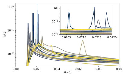
In practice, EOS can exhibit behaviors between an idealized phase transitions and merely sharp features, which also makes any semi-analytic approach ambiguous. In Fig. 1, we show the problematic term for a selection of nuclear physics EOS models (see Sec. IV.1). Although these contain only very weak phase transitions, the resulting peaks are quite sharp and difficult to resolve. In order to circumvent this problem altogether, we will now transform the ODE into a form that has regular coefficients at phase transitions and can be integrated using standard numerical methods.
We start by noting that the offensive term is closely related to the derivative of the density.
| (55) |
We can now simply cancel the degeneracy by using the density instead of the radius as independent variable.
| (56) | ||||
| (57) | ||||
| (58) |
From Eq. (51) and Eq. (52), we get
| (59) | ||||
Using the identity
| (60) |
we can rewrite the first term as
| (61) | ||||
Collecting terms, we find
| (62) | ||||
| (63) | ||||
The coefficients of the new ODE for are finite across phase transitions. They are also finite at the center, as follows from Eq. (46) and Eq. (53). Even if a phase transition happens exactly at the center, they remain finite. Although Eq. (63) contains a term which in this case diverges (see Eq. (53)) like , the coefficient in Eq. (62) remains finite.
At the surface, on the other hand, the term in the new ODE is now problematic, because the limit of zero density is not finite for all EOS. For example, it diverges for a polytropic EOS with (compare Eq. (18) and Eq. (19)).
To solve the problem near the surface, we derived yet another formulation, without sacrificing the good behavior at phase transitions. For this, we first change the dependent variable to
| (64) | ||||
| (65) |
The term in the integrand can be written as function of density since the density is strictly decreasing with radius for solutions of the TOV equations. The integrand is finite also at phase transitions, where it simply exhibits a plateau. The integration can thus easily be carried out numerically. The above subtraction eliminates the first term in Eq. (62), which becomes
| (66) |
Finally, we change the independent variable to , writing
| (67) |
The RHS given by Eq. (63) is completely unproblematic both at phase transitions and at the surface. The discontinuity in is now contained entirely in the variable . Although is smooth, and therefore have a jump at a phase transition.
As a crosscheck, we can recover the analytical contribution of a phase transition discussed in Postnikov et al. (2010); Takátsy and Kovács (2020). Denoting the density range of the phase transition by , the radial location by , and the constant enthalpy and pressure across the transition by and , respectively, we find
| (68) |
since the integrand in Eq. (65) is constant across the phase transition. Using , a straightforward computation yields
| (69) |
which agrees with Takátsy and Kovács (2020). A similar result in Han and Steiner (2019) seems to be intended to describe phase transitions near the surface and agrees in the limit of small .
Normally, the above ODE behaves well also at the center. Only in the rare case where the central density coincides with a phase transition, the coefficient diverges like (compare Eq. (53)). To sidestep this remaining problem, we use the formulation given by Eq. (62) to integrate up to some radius inside the star, and then switch to the formulation given by Eq. (67) to integrate up to the surface.
II.5 Moment of Inertia
The moment of inertia of uniformly rotating NS in the slow rotation limit was derived in Hartle (1967). This involves the solution of an ODE for a function related to frame dragging, with coefficients determined by the TOV solution describing the nonrotating NS. In detail,
| (70) |
Compared to the form in Hartle (1967), we inserted Eq. (30) and Eq. (31). To solve the ODE, we first transform it into an equivalent first order ODE using as independent variable
| (71) | ||||
| (72) |
Another variable transform leads to a form that can be integrated simultaneously with the TOV equations
| (73) |
where is given by Eq. (39).
The coefficients of ODE Eq. (70) are degenerate at the center, and the solution has just one degree of freedom given by . Using a Taylor expansion, one can show that the solution for in the limit is
| (74) |
As shown in Hartle (1967), the function outside the star is related to the angular momentum of the NS and its angular velocity as seen from infinity, , by
| (75) |
As a consequence,
| (76) |
which is unambiguous since is twice differentiable also across the NS surface. Combining the equations above, we compute the moment of inertia using the expression
| (77) |
Compared to Hartle (1967), this avoids another integration step.
II.6 Baryonic Mass, Binding Energy, Volume
The baryonic mass within a radius is given by the integral
| (78) | ||||
| (79) |
where we use the coordinates Eq. (29).
The total baryonic mass of a NS, , is important in the context of binary neutron star mergers. The law of baryon number conservation implies that the total baryonic mass of the system after merger is given by the sum of the baryonic mass of original coalescing NS. This can be used to relate the stability of the remnant to the EOS.
The binding energy of a NS is usually defined as . We note that this definition is a slight misnomer since is not exactly the energy difference between the ADM energy of a NS and a spacetime where the same amount of matter is infinitely dispersed. That would only be the case if each baryon contributes an energy given by the arbitrary constant for the dispersed state, whereas the actual value would depend on the nuclear composition of the matter.
Another quantity we compute is the proper volume enclosed within spherical surfaces of radius , which is given by
| (80) |
The proper volume of the NS is then given by . We are unaware of existing results providing outside the star, and derived the analytic expression below using straightforward integration.
| (81) | ||||
It is convenient to compute and while solving the TOV ODE instead of using a separate integration step. For this purpose, we can cast Eq. (78) and Eq. (80) into the differential equations
| (82) | ||||
| (83) |
For , we find
| (84) |
The advantage of this form is that the quantities and grow linearly with near the origin and the RHS of Eq. (82) and Eq. (83) remains finite.
II.7 Bulk measures
The proper volume is rarely used, which is surprising since it is a fundamental geometric property of any body, not restricted to spherical symmetry. This was utilized in the context of BNS merger remnants in Kastaun et al. (2016). To define measures applicable to any spacetime, one can use proper volume and baryonic mass enclosed within isodensity surfaces . One can also define an volumetric radius as the radius of the Euclidean sphere with equal volume. This allows to define a compactness measure . Although merger remnants lack a clearly defined surface, there is always one surface of maximum compactness , denoted as the bulk surface in Kastaun et al. (2016). This gives rise to definitions of bulk proper volume and bulk baryonic mass .
The same measures can easily be applied to a TOV solution, where the isodensity surfaces are just spheres . For a static NS, the formula given in Kastaun et al. (2016) to determine the bulk surface simplifies to
| (85) |
The bulk measures above are used in Kastaun et al. (2016) to compare the cores of TOV and merger remnants in a well-defined way. In detail, one can search for the intersection between the proper mass-volume relation of the remnants isodensity surfaces and the bulk mass-volume relation for the sequence of TOV solutions. If it exists, the corresponding TOV solution is called TOV core equivalent, because its bulk has a similar radial mass distribution than the merger remnant core.
II.8 Stable Circular Orbits
It is a well known fact that circular orbits of massive test particles in the Schwarzschild metric are unstable at radii smaller than the innermost stable circular orbit (ISCO) located at . Since the metric outside a spherical NS is the Schwarzschild metric, all orbits outside the NS surface are given by the latter. Therefore, all NS with compactness have an ISCO. Realistic NS models do indeed have an ISCO above some mass that depends on the EOS.
We could not find any reference regarding the stability of geodesics inside NS. This seems a somewhat academic question, but might be relevant when studying accumulation of particle dark matter inside NS. Below, we provide a short discussion of subsurface orbits. Interestingly, it turns out that NS with an ISCO also have an outermost stable internal circular orbit (OSICO in the following).
We start by setting up the usual geodesic invariants. For the line element Eq. (29), both and are Killing vectors. For a geodesic curve , we find the invariants
| (86) | ||||
| (87) |
where we have assumed that the curve is parametrized such that . From the above, it immediately follows that
| (88) | ||||
| (89) |
For a given angular momentum , the minima of the effective potential correspond to stable circular orbits, and the maxima to unstable circular orbits. It is trivial to compute
| (90) |
The condition yields the angular momentum for circular orbits at radius
| (91) |
Note that there is no circular orbit if . This happens for the Schwarzschild metric below (the location of the photonsphere). For simplicity, we will ignore the potential corner case of NS with or NS that violate anywhere within the interior. We can thus assume the existence of circular orbits at any radius inside a NS.
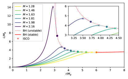
Next, we discuss the stability of the internal circular orbits. For a given , the roots of are the extrema of . Starting from the origin, the first root must correspond to a minimum since for . If there is a second root, it corresponds to a maximum (for the latter case, there must be a third root since for ). Therefore, circular orbits in the interval are stable, where is the location of the first maximum of within the star. Further, cannot have a maximum at the surface, where (still assuming ). The behavior of is illustrated in Fig. 2 for one EOS and different masses. To conclude, we find that NS with feature an ISCO outside the star and an OSICO located strictly below the surface.
We now turn to the orbital angular velocity of test particles on circular orbits. A general expression valid for axisymmetric stationary spacetimes can be found, e.g., in Laarakkers and Poisson (1999). Using Eq. (29) and Eq. (31), we can specialize to the spherical NS case to obtain
| (92) |
Outside the star, this simplifies to
| (93) |
Curiously, the orbital velocity assumes a nonzero value at the center. We are unaware of a corresponding formula in the literature, but it is trivial to derive. Using Eq. (46) and Eq. (92), we obtain
| (94) |
This provides a rough scale for the rotational velocity at which one should expect strong deformation of the core. For example, numerical merger simulations have found differential rotation profiles where the core is rotating much slower than the central orbital velocity, and radial mass distributions very similar to a nonrotating NS Kastaun and Galeazzi (2015); Kastaun et al. (2016, 2017).
III Implementation
In the following, we provide important technical details for the numerical implementation of the equations given in the previous section.
III.1 Avoiding numerical problems
The use of finite precision arithmetic can lead to severe accuracy problems. There are several places in our implementation where cancellation errors would lead to a catastrophic loss of accuracy with a naive implementation of our analytic formulas.
To avoid such a problem, we generally represent the pseudo-enthalpy in terms of . We recall that for . At low density, computing or would be inaccurate when using directly. Further, when evaluating the function for small arguments, we use a numerical implementation, denoted here as , that is accurate for , such that . Evaluating directly with finite precision arithmetic would result in catastrophic loss of accuracy.
Another type of problem is the correct treatment of ODE coefficients at boundaries. The coefficients of the TOV ODE in our formulation are finite and continuous when evaluated along a solution of the ODE. At the expressions Eq. (39), Eq. (40) are, however, only defined as a mathematical limit and cannot be evaluated numerically. Instead one has to use the expression for the limit. Further, the partial derivatives of the coefficients with respect to and diverge at the origin. This leads to a reduction of the convergence order for the first ODE integration step at the origin. When using an RK4/5 integration scheme with adaptive step size control, the impact on the global accuracy that can be achieved with given costs is small. However, we find that the maximum convergence order that can be reached with a fixed step size is limited to second order.
In our implementation, we evaluate the problematic term as follows
| (95) |
Above, denotes the stepsize when using fixed-step integrator, and when using an adaptive step size control. The error caused by using the approximation defined in Eq. (47) is of order . This limits the maximum convergence order for the ODE solution with fixed step size to 3rd order (one order higher than the error of the local RHS coefficient because it is integrated over the first step only). Compared to the order reduction present when using the exact formula, using the approximation thus increases the possible convergence order by one.
The integration of the moment of inertia ODE is mostly unproblematic, except for the term in Eq. (71). For , we use the analytic limit given by Eq. (74). Small on the other hand are not a problem because grows linearly from .
When integrating Eq. (62), there is one term which needs special care when evaluated numerically in the limit , although analytically it is finite
| (96) | ||||
First, we use as dependent ODE variable instead of . Otherwise the term would suffer catastrophic loss of accuracy for (where ) due to cancellation errors. Second, when evaluating the term above at , we use the analytic limit.
To compute proper volume and baryonic mass of a NS, we use the ODEs given by Eq. (82) and Eq. (83), using Eq. (84) when . The choice of dependent variables is more suitable for adaptive ODE solvers since they grow linearly with , in contrast to the straightforward ODEs for and . Using the binding energy instead avoids cancellation errors in the Newtonian limit (which is not a problem for NSs, but might be useful as a test case).
A third type of potential problems is the behavior of EOS and ODEs for NS properties at phase transitions. The problems with degenerate ODE coefficients are already taken care of by our analytical formulation, which also largely alleviates problems caused by inaccurate numerical representations of an EOS across a phase transition. Below, we provide the technical details of the corresponding implementation.
In order to compute the function defined in Eq. (65), we first perform a numerical integration based on the sample points obtained during the numerical solution of the TOV ODE. This step is not problematic since the integrand is finite and continuous everywhere, including the origin, the surface, and phase transitions. However, we found it necessary to use a 3rd-order accurate integration method (based on local quadratic interpolation) in order to not restrict the overall convergence order. The result of the integration is then used to construct a monotonic interpolation spline for . We also construct interpolation splines for and as functions of . It is important to interpolate instead of and , in order to avoid amplification of interpolation errors for . Using those splines and the EOS allow to evaluate Eq. (62) and Eq. (63).
To compute the tidal deformability, we use Eq. (62) to integrate from the central density to some lower density, compute using Eq. (64), and then use Eq. (67) to integrate to the surface. The exact matching point is not important, as we shall see. By default, our implementation uses .
We remark that Eq. (62) requires that the EOS implementation can accurately compute across a phase transition, whereas Eq. (67) does not even use . As long as the phase transition is below the matching density used for a given NS model, one can compute the tidal deformability accurately even if the EOS implementation does not resolve the sound speed across the phase transition.
It is also worth pointing out that it is much more difficult to numerically represent as function of than to represent it as function of , in particular when using interpolation of tabulated data. The reason is that merely stays zero over an interval, while for the entire phase transition is represented by a single point. Integrating the standard formulation Eq. (51) of the ODE across a phase transition would not just require some specialized ODE solver, but also require a special EOS implementation able to represent extremely sharp features in the soundspeed .
Another formula affected by large cancellation errors is Eq. (50), as was pointed out in Postnikov et al. (2010). When applied to stars with compactness much lower than typical NS, such as white dwarfs, several orders of the terms polynomial in cancel with the logarithmic term, as can be seen by Taylor-expanding it. The problem becomes manifest when testing our initial implementation on unrealistic polytropic EOS that result in stellar models with compactness .
In Postnikov et al. (2010), one can find an approximation based on Taylor-expansion that solves the cancellation problem. However, by numerical comparison to the exact formula in the regime where both approximation and exact formula are accurate, we find that the expansion contains several faults. We therefore re-derived the expansion in . For this, we approximate the love number as a polynomial as follows
| (97) |
Expanding the master equation Eq. (50) in powers of , we obtain the coefficients
| (98) | ||||
| (99) | ||||
| (100) | ||||
| (101) | ||||
| (102) | ||||
| (103) | ||||
| (104) | ||||
| (105) | ||||
| (106) |
We verified numerically that this expansion converges to the exact formula with error until the numerical cancellation errors start to dominate. For the final numerical implementation, we use
| (107) |
Here is a threshold value chosen based on plots of comparing exact expression and approximation formula. Further, and are the exact and approximate expressions given by Eq. (50) and Eq. (97). The addition of the sixth-order term proportional to the difference between the two at the threshold value reduces the error further, although it remains of order .
III.2 Interpolating EOS
For EOS provided only at sample points, some form of interpolation is required. The interpolation method needs to be monotonic in order to prevent overshoots that violate Eq. (7). It is also desirable that the interpolated functions are differentiable because otherwise the convergence order of any ODE solver drops as soon as the ODE step becomes comparable to the EOS sampling resolution. The sample points should cover many orders of magnitude in density and therefore is is best to perform the interpolation in logarithmic space. Finally, the numerical costs of interpolation should ideally not increase with number of sample points. To satisfy all those requirements, we use a monotonic cubic spline interpolation of , , , , and . The samples are spaced regularly in or . We interpolate in terms of instead of because it is impossible to resolve a phase transition for the latter case since it corresponds to a single point in but a range in . From the above interpolating functions, we consistently compute and .
EOS samples are typically not provided with the particular spacing described above. We therefore perform another interpolation step to create the required regularly spaced samples from the available ones. This is done as described above, only that we use a slower variant of the monotonic spline interpolation that allows non-regular spacing.
Often, EOS samples are only provided above some low density cutoff. Further, it is generally wasteful to use a large number of sample points for densities too low to have any impact on NS properties. Therefore, we restrict the range for interpolation above a suitably chosen cutoff density, which may be equal or larger than the lowest available sample point. Below the interpolated range, we attach a polytropic EOS using the matching conditions Eq. (21).
When solving TOV equations, the EOS is required down to zero density in order to reach the NS surface. Ideally, the sampled region extends to low enough densities such that the exact choice for the extrapolation to low densities does not matter. We will investigate this in Sec. III.4. In any case, the prescription provides a clearly defined EOS.
We note that it is much easier and more consistent to first extend an incomplete EOS to zero density than to add various technical workarounds during the computation of NS properties. Using workarounds in the TOV solver is either inconsistent or equivalent to some extrapolation of the EOS, with the disadvantage of not being made explicitly.
III.3 Testing ODE Solutions
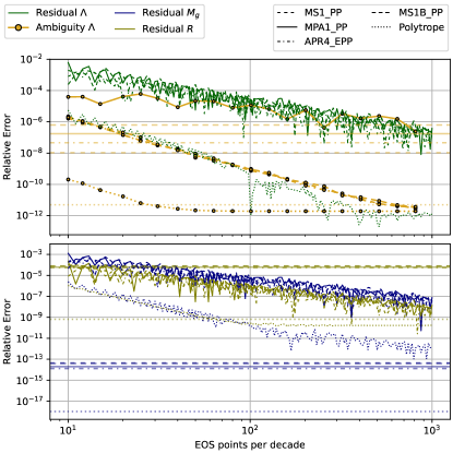
In order to assess the accuracy of the numerical ODE solutions, we first study the convergence behavior for the simple case of integrating the ODEs using fixed step size, employing a RK4/5 integrator. We use twice as many points for the tidal ODE than for the TOV ODE. We recall that TOV and tidal ODEs use different independent variables and therefore the integrations steps for each ODE are not constant in terms of the independent variable of the other ODE. The factor of two was determined by roughly optimizing computational costs at a given accuracy.
We are varying the step size for the TOV solution from 10 to 10000 points within the NS. As an estimate for the ODE integration error, we compute the residuals of NS properties with respect to an even higher resolution of 100000 points.
We perform this test for many different EOS, each time for a NS model with and for the maximum mass model. We use EOS from three different categories. The first group consists of 24 nuclear physics EOS represented as monotonic spline interpolation of tabulated data. Those EOS are described in Sec. IV.1. The second group consists of piecewise polytropic approximations of the MPA1 and MS1 EOS. The last group contains polytropic EOS with polytropic indices in the range . The polytropic constant is chosen such that the maximum mass is .
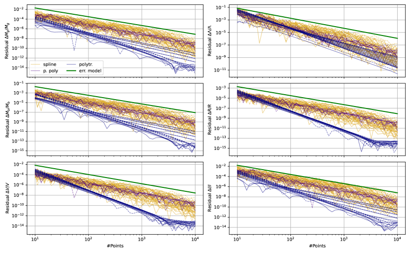
Fig. 3 shows the residuals for gravitational mass, baryonic mass, circumferential radius, proper volume, moment of inertia, and the tidal deformability. We find that the solutions converge with increasing resolution, but the convergence rate varies between the EOS, and the absolute error differs strongly. Not surprising, the errors are, on average, lowest for the analytic polytropic EOS. The piecewise polytropic EOS show slower convergence, which we attribute to the fact that they are not differentiable across the segment boundaries. For the spline-based EOS, we observe a somewhat more noisy convergence behavior. This might be caused by the interplay between the locations of ODE integration steps and EOS interpolation sample points. Further, some of those EOS exhibit relatively sharp features in the sound speed (see Fig. 1). Although those are not problematic, thanks to our choices of analytic formulations, they can still cause a non-constant convergence rate.
We note that for some of the polytropic models, the tidal deformability fails to converge in this test unless the love number is computed using our improved implementation Eq. (107) instead of Eq. (50). The reason is that the compactness of those models decreases rapidly with polytropic index, leading to models more similar to white dwarfs than neutron stars, thus triggering the cancellation errors present for low compactness in the naive implementation.
For practical purposes, it is important that users can specify the desired accuracy instead of technical details such as step size. For this, our implementation uses power laws for the residuals of each NS property as function of step size. Those power laws are chosen based on our test results, and are shown in Fig. 3. The exponents are for the deformability and for all other quantities. Those bounds are intended as heuristic estimates of the required resolution. We emphasize that one still needs to perform a convergence test for a given model if reliable error bounds are required.
Our results show that the accuracy for fixed step size can vary by orders of magnitude between different EOS. This suggests that an adaptive step size might be more efficient. More importantly, adaptive step size methods might reach the prescribed accuracy also for corner cases not covered in our selection of test cases. However, adaptive methods have one shortcoming for our use-case. We recall that we first solve the TOV equations, while the ODE for the tidal deformability is solved in a subsequent step. Using an adaptive step size for the TOV equations will only reduce the step size as needed for those equations. The tidal ODE might require finer resolution of the TOV solution in very different locations, in particular at densities where the sound speed has sharp features.
For our main general-purpose implementation, we use a hybrid approach for the step size selection. Both for TOV and tidal ODE, we employ a RK4/5 ODE integrator with adaptive step size control. However, if the computation of the deformability is requested, we also enforce a minimum resolution for the integration of the TOV ODE. This resolution is based on the heuristic power law error model found for the fixed step size tests above. Since ODE integration errors become less predictable in the low-accuracy regime, our implementation also employs a lower resolution limit.
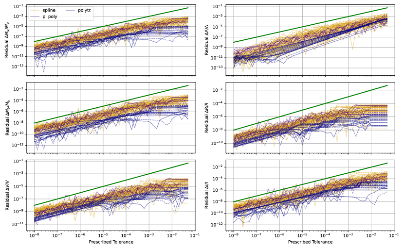
In order to measure the accuracy and to calibrate the adaptive step size control, we solve the same models as for the previous test, but using different values for the local tolerance used in the step size control. We then use simple constant scale factors to chose the local tolerance based on the desired global errors for the different NS properties. This allows to specify the desired accuracy for each quantity separately. Fig. 4 shows the prescribed accuracy for each property in comparison to the measured residual (again with respect to a much higher resolution). As one can see, almost all models achieve the prescribed accuracy. As a trade-off between reliability and efficiency, we deliberately did not chose the calibration factors large enough to cover the few outliers. The error model is intended as a heuristic guideline valid for typical EOS covered by our test cases. If more exact error bars are required, one should always perform a dedicated convergence test for the model at hand.
III.4 Testing the Impact of EOS Approximation
Our next test concerns the inaccuracies introduced by approximating a given EOS using monotonic spline interpolation. For this, we interpolate several analytic EOS with increasing number of sample points and compute the residuals of NS properties with respect to the original EOS. The EOS used for this test are two piecewise polytropic EOS and one simple polytropic EOS.
The residuals for mass, radius, and deformability are shown in Fig. 5. We find that the polytropic EOS is approximated much more accurate by the interpolation spline, and converges faster. This is not surprising since the piecewise polytropic EOS is not differentiable at the segment boundaries, while the polytropic one is differentiable everywhere.
However, for the polytropic case we also find that the residual of the radius does not decrease with resolution below a value of . As it turns out, the reason for this behavior is that our implementation of the interpolating EOS uses a matching polytropic EOS below a given low density threshold , in our example at . The polytropic index of this polytrope is chosen as for this test. This is the same value as the lowest segment of the piecewise polytropic examples, whereas the purely polytropic EOS has a different index of . At low densities, the polytropic example EOS is misrepresented, while the other two EOS are represented exactly.
We can easily obtain an estimate for the error introduced by the low-density approximation. Near the surface, we can assume . Equations Eq. (39), Eq. (32), and Eq. (35) then yield the approximation
| (108) |
where . This allows to compute the thickness of the shell with density below . We find
| (109) |
When using the polytropic approximation below , and assuming that , we obtain
| (110) |
The error in the NS radius caused by approximating the low density regime is given by the difference of obtained from Eq. (109) for original and approximating EOS. Computing from Eq. (110) already provides a useful estimate for the magnitude of the potential error, even though it is not a strict upper bound. The results from the above error estimates are shown in Fig. 5 as well. We find that the estimate for the polytropic case roughly agrees with the observed limitation of the NS radius accuracy.
It is worth pointing out that the error estimate for the other examples is many orders of magnitude larger, even though the matching density was the same in all cases. The actual error for this example is small compared to the estimate, but only because the low-density polytropic approximation happens to agree exactly with the original EOS. In general, however, this source of error needs to be taken into account.
The reason for the larger potential error is that the low-density behavior of the polytropic example is very different from the other examples. The polytropic constants was chosen such that the maximum NS mass is . As it turns out, the resulting differs by orders of magnitude from the polytropic constant of the lowest segment for the two piecewise polytropic EOS. The latter are representative for realistic nuclear matter EOS, for which the low-density behavior is relatively well constrained.
When processing many EOS from different sources, it is desirable to automate the conversion into a spline representation. For this, one may decide to always use the same low-density polytropic approximation mimicking realistic nuclear physics EOS, and to use the same matching density . We can find an appropriate universal matching density using Eq. (110)
| (111) |
where is the desired accuracy of the radius, and is the lowest compactness that will be considered. When using a low density polytrope with and , we obtain a matching density appropriate for and .
In contrast to the radius, the mass is not significantly affected by the low-density behavior of the EOS. Approximating the TOV equations near the surface, we obtain an estimate for the mass in the low density shell as
| (112) |
The result for our examples is shown in Fig. 5. As one can see, the impact on the mass is negligible.
Finally, we note that the use of interpolation splines to approximate EOS does not just introduce an error, but an ambiguity. The reason is that is not exactly the inverse function of , and thus one obtains slightly different results depending on which is used. One such ambiguity is manifest in our implementation of the deformability. We recall that we use two different formulations, one based on and one based on , switching between the two at some point inside the star. To measure the above ambiguity, we use the standard deviation of computed for 25 different choices (regularly spaced in ) for the location of the transition point. Fig. 5 shows the ambiguity versus the EOS sampling resolution. Again, we find much lower values for the polytrope. We also find that the ambiguity varies strongly within the piecewise polytropic examples, for unknown reasons.
IV Application
IV.1 Example EOS collection
As part of our EOS handling framework, we provide a small collection of EOS files. The aim of this collection is twofold. First, we use it for our tests of the library. Second, it provides a convenient starting point for exploring various NS related questions for a variety of EOS. The chosen set constitutes a representative selection of nuclear physics EOS models. For a more extensive collection of EOS data, we refer to Typel et al. (2018). The full list of available EOS is given in Table 1 together with the maximum mass TOV solutions (see next section). The EOS files are available in Kastaun (2024b).
In detail, our selection includes the EOS considered in Abbott et al. (2020). Those EOS are based on tables available in the literature on nuclear physics EOS modeling, but have been sanitized by removing clearly faulty samples, limiting the validity range to respect causality, resampling coarsely sampled tables, and supplementing missing low-density data. Some EOS have also been replaced by analytic piecewise polytropic approximations from Read et al. (2009) because the original tables were sampled too coarsely for unambiguous interpolation. For details, we refer to Abbott et al. (2020).
Our EOS framework supports piecewise polytropic EOS natively. However, we also sampled some piecewise polytropic EOS to obtain representations based on spline interpolation. This was done only for testing purposes and the sampled variants are not used in the following sections.
The EOS used here are as close to the ones from Abbott et al. (2020) as possible, but have been resampled to the regularly spaced values employed by our EOS implementation. Note that the EOS data used in Abbott et al. (2020) was already resampled from the original sources to a suitable common resolution. Our example set is therefore not the closest possible representation of the original data, in particular with regard to sharp features, such as weak phase transitions.
IV.2 Properties of NS for Common EOS Models
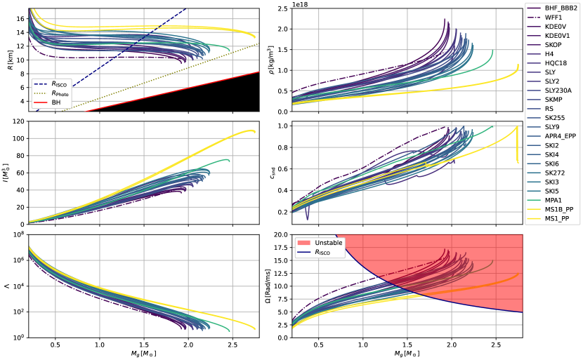
As a first application of our code infrastructure, we compute the sequences of TOV solutions for our collection of EOS. Fig. 6 shows the properties of stable NS as function of gravitational mass (up to the maximum).
As one can see from the mass-radius relations, none of the sequences have a photonsphere, i.e. allow circular photon orbits outside the star. Further, all of the TOV sequences in our selection develop an ISCO before reaching the maximum mass. This can also be seen from the panel showing the angular velocity of circular orbits at the NS surface in comparison to the one at the ISCO radius. In general, the surface orbital angular velocity increases with mass for our selection. Once it crosses the ISCO angular velocity, which decreases with mass, the surface orbits are unstable.
The panel showing the central density is useful to interpret EOS constraints from GW observations, since the signal cannot be influenced by the EOS at densities above the central ones for given range of involved NS masses. Of course, it is still possible to infer constraints on the pressure beyond those densities, using the causality constraint on the speed of sound. The mass-density plot also shows that the maximum NS mass and the central density of the corresponding NS are anticorrelated for our selection.
The mass-central soundspeed relation plot exhibits non-monotonic behavior as well as sharp features. The reason is simply that EOS can have a non-monotonic soundspeed-density relation and sharp features. For the same reason, the maximum sound speed inside a NS is not always the central value.
Fig. 6 also shows the moment of inertia. For any search for GW from single rotating NS, the moment of inertia is an important quantity as it relates GW amplitude, GW frequency, and spindown rate (for GW-dominated spindown). The plot can be used to assess the error made when using ballpark figures for typical NS. It also shows that maximum mass and maximum moment of inertia are strongly correlated.
The mass-deformability plot shows that the maximum mass models for our selection generally have a low tidal deformability of order 10. For current ground-based detectors, those maximum mass NS models are therefore near undistinguishable from BH. This seems to be mainly related to the high compactness of the maximum mass models for our EOS selection. As we will see in Sec. IV.5, one can easily construct EOS that have mass maxima with lower compactness and much higher tidal deformability.
For each EOS, the NS model of maximum mass is of particular interest. Table 1 provides gravitational mass , baryonic mass , proper circumferential radius , moment of inertia , central baryonic mass density , and central sound speed . In addition, we compute novel measures introduced in Kastaun et al. (2016), dubbed “bulk mass” and “bulk compactness” (see Sec. II.7). The bulk measures of the maximum mass TOV solution may be useful because they appear in a recently proposed empirical criterion for post-merger BH formation Ciolfi et al. (2017); Endrizzi et al. (2018); Kastaun and Ohme (2021). We checked that our results on the maximum masses are consistent with the ones reported in Abbott et al. (2020).
Next, we compute NS properties at a fiducial mass . Table 2 provides baryonic mass , proper circumferential radius , central baryonic mass density , moment of inertia , the angular velocity of internal circular orbits near the center according to Eq. (94), and dimensionless tidal deformability . In addition, we provide the first derivative
| (113) |
evaluated at .
Expanding the logarithmic tidal deformability around the fiducial mass to first order might be sufficient for many applications. For example, De et al. (2018) analyzed the GW data for the single event GW170817 assuming a constant slope of for all EOS and kept only the deformability at some fiducial mass as a free parameter. This approximation thus reduces the infinite-dimensional space of EOS to a single degree of freedom. Once there are further constraints on at different masses from future observations, it will become possible to constrain two degrees of freedom, which can be expressed in terms of and at some fixed fiducial mass. We caution that Taylor expansion (to any order) ceases to be a viable approach when considering EOS that lead to multiple stable NS branches. This case will be discussed in Sec. IV.5.
| EOS | ||||||||
|---|---|---|---|---|---|---|---|---|
| BHF_BBB2 Baldo et al. (1997) | ||||||||
| WFF1 Wiringa et al. (1988) | ||||||||
| KDE0V Gulminelli and Raduta (2015); Agrawal et al. (2005); Danielewicz and Lee (2009) | ||||||||
| KDE0V1 Gulminelli and Raduta (2015); Agrawal et al. (2005); Danielewicz and Lee (2009) | ||||||||
| SKOP Gulminelli and Raduta (2015); Reinhard et al. (1999); Danielewicz and Lee (2009) | ||||||||
| H4 Lackey et al. (2006) | ||||||||
| HQC18 Baym et al. (2018) | ||||||||
| SLY Douchin and Haensel (2001) | ||||||||
| SLY2 Gulminelli and Raduta (2015); Danielewicz and Lee (2009) | ||||||||
| SLY230A Gulminelli and Raduta (2015); Chabanat et al. (1997); Danielewicz and Lee (2009) | ||||||||
| SKMP Gulminelli and Raduta (2015); Bennour et al. (1989); Danielewicz and Lee (2009) | ||||||||
| RS Gulminelli and Raduta (2015); Friedrich and Reinhard (1986); Danielewicz and Lee (2009) | ||||||||
| SK255 Gulminelli and Raduta (2015); Agrawal et al. (2003); Danielewicz and Lee (2009) | ||||||||
| SLY9 Gulminelli and Raduta (2015); Danielewicz and Lee (2009) | ||||||||
| APR4_EPP Read et al. (2009); Akmal et al. (1998); Endrizzi et al. (2016) | ||||||||
| SKI2 Gulminelli and Raduta (2015); Reinhard and Flocard (1995); Danielewicz and Lee (2009) | ||||||||
| SKI4 Gulminelli and Raduta (2015); Reinhard and Flocard (1995); Danielewicz and Lee (2009) | ||||||||
| SKI6 Gulminelli and Raduta (2015); Nazarewicz et al. (1996); Danielewicz and Lee (2009) | ||||||||
| SK272 Gulminelli and Raduta (2015); Agrawal et al. (2003); Danielewicz and Lee (2009) | ||||||||
| SKI3 Gulminelli and Raduta (2015); Reinhard and Flocard (1995); Danielewicz and Lee (2009) | ||||||||
| SKI5 Gulminelli and Raduta (2015); Reinhard and Flocard (1995); Danielewicz and Lee (2009) | ||||||||
| MPA1 Müther et al. (1987) | ||||||||
| MS1B_PP Müller and Serot (1996); Read et al. (2009) | ||||||||
| MS1_PP Müller and Serot (1996); Read et al. (2009) |
| EOS | |||||||
|---|---|---|---|---|---|---|---|
| BHF_BBB2 | |||||||
| WFF1 | |||||||
| KDE0V | |||||||
| KDE0V1 | |||||||
| SKOP | |||||||
| H4 | |||||||
| HQC18 | |||||||
| SLY | |||||||
| SLY2 | |||||||
| SLY230A | |||||||
| SKMP | |||||||
| RS | |||||||
| SK255 | |||||||
| SLY9 | |||||||
| APR4_EPP | |||||||
| SKI2 | |||||||
| SKI4 | |||||||
| SKI6 | |||||||
| SK272 | |||||||
| SKI3 | |||||||
| SKI5 | |||||||
| MPA1 | |||||||
| MS1B_PP | |||||||
| MS1_PP |
IV.3 Multimessenger Applications
As another simple application of our code, we consider the case of a multi-messenger BNS merger detection where EM counterparts point to the formation of a BH. We will discuss some simple consequences of the assumption that a BH was formed, which would need to be considered in Bayesian parameter estimation and model selection studies of the GW data.
For a given EOS, we can easily compute the total baryonic mass of the system from the gravitational masses of the constituents, as parameterized by chirp mass and mass ratio . For simplicity, we assume that spin effects can be neglected. It is also straightforward to compute the total baryonic mass that can be contained in a single nonrotating NS. It is a safe assumption that the remnant is a stable NS if the total baryonic mass is below the above value. We note that although a priori the merger could still produce a BH by some dynamical effect, we are not aware of any such example from numerical relativity simulations. It should also be noted that BNS merger remnants have considerable angular momentum and can therefore support masses larger than the maximum for nonrotating NS, forming a long-lived supramassive remnant.
In Fig. 7, we show the resulting lower chirp mass limit for BH formation as function of mass ratio. For comparison, we show the estimate for the chirp mass in GW event GW170817 Abbott et al. (2019a). For this and similar events, the chirp mass can be constrained so well that for our discussion we can assume it to be known exactly. From the figure, we can read off immediately that the knowledge of the chirp mass can place strong constraints on the mass ratio, if the EOS is given. Under the assumption that a BH has formed the possible mass ratio drops rapidly once the chirp mass drops below a critical (EOS-dependent) value. The BNS mass ratio is an important nuisance parameter in GW parameter estimation studies aiming to constrain the EOS. Hence it might be beneficial to include the assumption of BH formation in the prior, by excluding at least the region below the aforementioned chirp mass limit. Of course, the correct approach is to use estimates for BH formation thresholds instead of simple lower limits, which could be obtained from numerical relativity simulations.
Computing the excluded region in the mass prior requires knowledge of the EOS. For Bayesian model selection studies, the EOS is given. For parameter estimation studies employing parametrized EOS, one needs to consider a different mass prior for each EOS. In other words, the assumption of BH formation introduces an additional correlation between priors for masses and EOS parameters, besides the existence of a maximum NS mass.
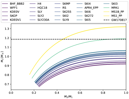
IV.4 Universal Relations for GW
There are several observational avenues for constraining the EOS of NS matter. A detection of GW from a BNS coalescence mainly provides constraints in the plane (setting aside complications when allowing for rapid spins or unequal masses) but no direct information on the radius (this might change once a signal from the merger itself can be observed). Electromagnetic observations such as NICER Bogdanov et al. (2019); Gendreau et al. (2016) provide constraints in , but no direct measurement of .
Both and depend on the EOS, so it is —in principle— possible to obtain combined EOS constraints in a fully consistent Bayesian manner. The difficulty lies in the nontrivial parametrization of the EOS uncertainties and the requirement for fully self-consistent prior assumptions.
The situation would be much simpler if radius and deformabilty would depend on the EOS in the same way. In detail: for a given mass, each possible EOS corresponds to a point in the plane. Let us assume that the set of those points does not constitute a two-dimensional region, but is constrained to some one-dimensional curve (or at least a sufficiently narrow band). Further, assume that this curve can be described as a monotonic function . One can then convert measurements of into measurements of , and vice versa, without considering the EOS.
There are several proposals for such EOS-independent relations (universal relations) Yagi and Yunes (2017); De et al. (2018) given as a functional relation , where is the compactness. We note that this relation is more restrictive than required. For the purpose of simplifying combined data analysis, it would be sufficient to have a relation for each mass , whereas the above universal relation is the same for all masses.
Both universal relations from Yagi and Yunes (2017); De et al. (2018) are derived as fits to a small selection of EOS models predicted by nuclear physics. Even for those EOS models considered, the relations have considerable residuals and can be called quasi-universal relations at best. This can be seen in Fig. 8 showing the relation computed with our code for many nuclear physics EOS. Instead of , we show the equivalent relation . As one can see, neither universal relation fits the band spanned by the EOS particularly well. The plot highlights that the “universality” of is simply owed to the factor in Eq. (49), i.e., the strong dependency on the compactness dominates other factors.
Using the universal relation to constrain the EOS from given observational data implies the assumption that the relation is respected by all EOS not yet ruled out by previous data, and not just by the selected examples used to establish the relation. In other words, any constraints on the EOS would already be based on assumptions about the EOS. We note that universal relations have already been used to convert deformability constraints into radius constraints in the context of gravitational wave event GW170817 Abbott et al. (2018); De et al. (2018).
Showing that the universal relations are truly universal in that sense is difficult. However, it is easy to answer the question whether the universal relations are a good approximation for all EOS, realistic or not. The set of polytropic EOS used for our tests provides counterexamples, as can be seen in Fig. 8. We stress that those polytropic EOS differ from the nuclear physics models already at low density, where the EOS is well constrained.
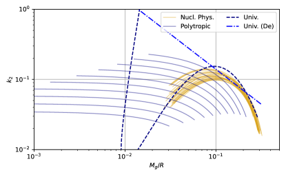
To get a more systematic measure for the universality of universal relations, we used our library to perform a numerical search for larger violations of said relations over a family of parametrized EOS. Our motivation is to get the universal relation violations under the simplistic assumption that the EOS at low densities is constrained by the spread of available nuclear physics models, while at high densities the EOS is completely unconstrained. The parametrized EOS we use to this end are based on modifying tabulated nuclear physics EOS only above a density threshold. For densities above , we replace the original speed of sound by a smooth monotonic interpolation between a small number of sample points at fixed energy densities. The parameter space of the EOS is simply given by the sound speeds at those points. From the speed of sound, the full EOS is constructed using Eq. (5) and Eq. (6) valid for isentropic (cold) EOS.
We then use a simple optimization scheme to look for the parameters with largest deviations from the universal relations. For this, we maximize a scalar function that computes the -norm of the compactness deviation as function of mass, weighted by a Gaussian mass “prior”. Doing so, we found that this can lead to parameters for which the maximum NS mass is well below . To suppress this region of parameter space, we multiply the scalar function by a penalty factor that is a smoothed-out step function in terms of the maximum NS mass. Another complication which emerged is the splitting of the stable NS branch into two, separated by an unstable branch. To account for this, we use the larger of the two mass maxima in the penalty factor for the maximum mass. Further, for a mass within the overlap of the mass ranges spanned by two branches, there are also two different values for the violation of the universal relation. We simply use the mean of the squares in the -norm of the scalar function we maximize.
We note that our maximization scheme is not designed to reliably find global maxima inside the multi-dimensional parameter space. Also note that we optimize the average violations and one could probably find larger violations for any given particular mass. Further, our EOS parametrization is not well suited to model phase transitions. As shown in Han and Steiner (2019), strong phase transitions can also have a significant effect on the deformability. The results of our search should therefore be regarded as examples that provide lower limits for the possible violations.
The results for parametrized EOS based on each of our nuclear physics EOS examples are shown in Fig. 9. For each EOS, it displays tidal deformabilty versus compactness for three selected masses, both for the original EOS and the corresponding parametrized EOS with the largest overall violation found by our search. As one can see, the deviations from the universal relations can be substantially larger than the spread of the original nuclear physics EOS. Our findings show that the compactness-deformability universal relations cannot be used in any study aiming to constrain the high-density part of the EOS, since obviously one already needs to assume EOS constraints to satisfy those relations.
It is instructive to compare the parametrized EOS members that violate the universal relations to the original EOS. This is shown in the bottom panel of Fig. 10. Apparently, decreasing the soundspeed at high density while increasing it at medium densities leads to the largest deviations found in our search. It should be noted that the spread surely depends on the density below which the EOS is kept constant. Our choice is pretty low, around one quarter of the nuclear saturation density. Hence, our results are not valid counterexamples against the use of universal relations for applications where the EOS is already assumed to be constrained by other means up to higher densities.
We remark that Fig. 9 highlights another problem with using the universal relations. As we already pointed out in Kastaun and Ohme (2019), the range of compactness at a given mass is limited, at least when considering only the EOS used to calibrate the universal relations. It is therefore not self-consistent to simply use universal relations of the form to convert a posterior probability density for that was obtained from some generic prior into a posterior for . For example, applying the universal relation from De et al. (2018) to a parameter sample with and is not meaningful because this region of parameter space is clearly excluded for all EOS models used to derive the universal relation (moreover, the resulting compactness exceeds that of a BH). Somewhere, one has to consider the limited range of for a given mass as well, ideally by incorporating the constraint into the multivariate prior probability density used for .
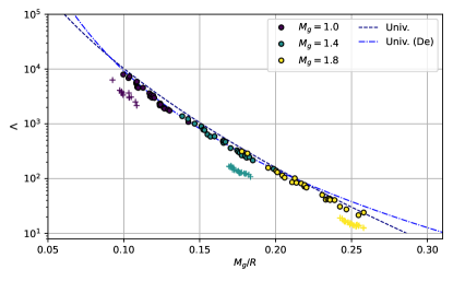
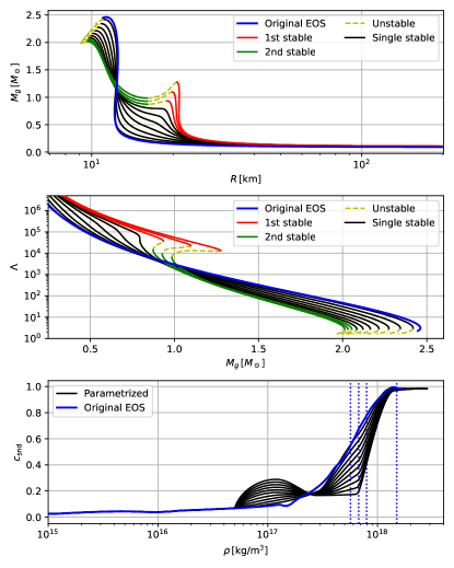
IV.5 Branch Splitting for Parametrized EOS
Our results for parametrized EOS indicate that the possibility of multiple stable branches needs to be taken seriously in parameter estimation studies using parametrized EOS. To emphasize this point, we visualized the branch structure along a one-parametric family of EOS connecting one of the nuclear physics EOS to the modified version with the largest deviation from universality, as shown in Fig. 10. The upper panel shows how, moving along this family, the single stable branch present for the original EOS first develops a plateau and then a second local maximum, thus splitting into two stable branches connected by an unstable one. To determine the stable and unstable branches, we use the mass-radius criteria from Bardeen et al. (1966) valid for cold NS EOS. As shown in the plot, the - curve bends counter-clockwise at the first local mass maximum, which means that one stable radial mode becomes unstable. At the subsequent local mass minimum, the curve bends clockwise, meaning that the single unstable mode becomes stable again. Finally, the second stable branch terminates at the second mass maximum, where the bend is counter-clockwise and a mode becomes unstable again.
We point out that the splitting of branches leads to a conceptual complication in parameter estimation studies using parametrized EOS. As shown in the middle panel of Fig. 10, the tidal deformability as function of mass becomes multi-valued where the mass ranges of the two branches overlap. To set up the multivariate prior for mass and deformability, even when just assuming a fixed EOS together with some mass prior, one now has to chose a branch for certain masses. This implies a physical assumption of how NS form. For example, one could assume that for a given mass, a NS is always located on the branch with lower central density. Or one could introduce a discrete “branch selection” prior instead. When assuming that both branches are allowed in some mass range, a further complication arises from the question which combinations are realized in a neutron star binary. The corresponding prior could just assume that each NS is randomly assigned a branch based on the single-NS branch prior, or it could introduce correlations incorporating models of binary formation channels. When using priors for mass and EOS parameters (which are not independent because of the maximum mass for each EOS) the prior for the tidal deformability is only fully determined after incorporating another prior for the selection of branches. The resulting full prior for mass, EOS, and deformability might become quite complex.
Fig. 10 also shows that the tidal deformability for a given mass can differ quite strongly between two branches. When assuming that a NS is always on the the lowest-density branch available for a given mass, it implies a discontinuity in . For an unequal mass binary, one cannot model the effective deformability anymore by approximating by a low-order Taylor-expansion. For the EOS in Table 2 however, there is just one stable branch, and the slope parameter remains useful.
Finally, we discuss how well GW observations from BNS coalescences can distinguish between the two stable branches. To estimate the order of magnitude of waveform differences, we use the post-Newtonian “TaylorF2” model Brown et al. (2007); Damour et al. (2001, 2002) as implemented in LALSimulation LIGO Scientific Collaboration (2024a). The agreement between signals is quantified by a noise-weighted inner product, or overlap Finn (1992). We assume Advanced LIGO’s design sensitivity Abbott et al. (2018); LIGO Scientific Collaboration (2024b) with lower cutoff frequency at .
Fig. 11 shows the mismatch (i.e., the overlap) between waveforms for an equal mass BNS coalescence that only differ in the tidal deformability parameter. For each BNS waveform, we assume that both NS follow the same EOS and are also on the same branch. We compare the two stable branches of the modified EOS shown in Fig. 10 that deviates most from the original one. In addition, we compare each of those branches to the single stable branch of the original MPA1 EOS.
Branch 1 (lower mass branch) of the modified EOS is characterized by very large tidal deformabilities, . These large values lead to a significant dephasing between signals assuming the original EOS and Branch 1, respectively, and also between the two branches of the modified EOS. This corresponds to mismatches that are significant for any SNR above the detection threshold. For example, is commonly used in the literature as a conservative mismatch threshold for indistinguishable signals Lindblom et al. (2008); Ohme et al. (2011). Conversely, a mismatch would start to become distinguishable already for SNRs . Therefore, if the EOS were known and similar to our example, ground-based detectors would be able to distinguish the two branches of the modified EOS example, and also between branch 1 of the modified EOS and the original EOS.
For masses in Fig. 11, Branch 2 (higher mass branch) of the modified EOS yields lower tidal deformabilities than the original EOS. The GW signals in this case are more similar and mismatches significantly lower (between and ). The signal differences in this regime only become distinguishable for SNRs between and .
We also considered the possibility of a BNS where the two NS are on different stable branch of the same EOS. Fig. 11 also shows the mismatch between the case where both NS are on the same branch and the case where each NS is on a different branch (still for equal masses). Not surprising, the mismatches are somewhere in-between the mismatch between branches when both NS are on the same branch.
These are order-of-magnitude estimates for an extreme example that do not take other parameter variations into account. Nevertheless, our considerations show that signal differences between the different branches may become observationally relevant in parameter estimation studies based on parametrized EOS. Any such study that aims to constrain the EOS therefore needs to incorporate the branch structure.
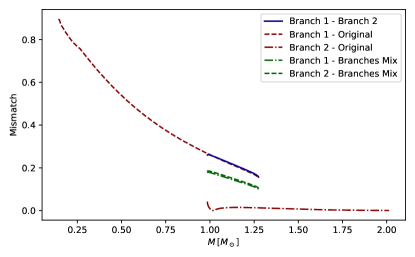
V Summary and Outlook
In this article, we collect everything required to compute the properties of nonrotating NS in GR. We provide novel analytic formulations of the tidal deformability differential equations that are robust when employing EOS with phase transitions. We also point out pifalls that occur in numerical implementations and how to avoid those.
The equations have been implemented in a publicly available library RePrimAnd. We demonstrate the accuracy of the solution and the robustness of the code using a wide range of example models. In addition, we used the convergence tests to set up a model of the error budget that was incorporated into the library, allowing users to specify the desired accuracy directly.
Our library makes it easy to compute NS models within C++ or Python code, or in an interactive Python environment such as Jupyter notebooks. Besides the NS functionality, the library also provides a consistent and generic interface to the use and exchange of various EOS models in a transparent manner. The aim of this library is to be useful for applications in GW data analysis involving NS, the testing of novel phenomenological relations between NS properties, for mapping novel EOS models to NS properties, and for initial data generation in numerical relativity.
As a first application, we compute properties of a typical NS with fiducial gravitational mass of for various EOS, including baryonic mass, radius, moment of inertia, and tidal deformability. We also provide the first derivative of the tidal deformability with respect to mass. This might be useful in BNS GW data analysis studies that reduce the EOS uncertainty to the values of tidal deformability and its derivate at some fiducial mass. Further, we compute the maximum mass models and their properties for each EOS. We also provide the corresponding EOS files for reference, as well as files with the TOV sequences. Those EOS and sequences are easily accessible through the Python interface of our library.
As a second application, we explore the reliability of universal relations between compactness and tidal deformability. We construct EOS for which those relations are violated much more than for nuclear physics EOS models. Those examples are based on nuclear physics EOS but modified above of the nuclear saturation density. They show that the universal relations can only be employed in situations where the EOS is already constrained to higher densities, but not for studies aiming to constrain the EOS without prior constraints.
As a third application, we demonstrate how the stable branch of a NS sequence splits into two branches when transitioning the EOS within a parametrized EOS family. We point out that this possibility needs to be taken into account on the technical level, but also requires addressing the physical model which branch NS with a given mass would occupy in nature. Further, we show that in such situations, it becomes infeasible to approximate the mass dependency of the tidal deformability using a Taylor expansion.
We show that branch splitting can cause significant differences in GW signals of BNS coalescence and demonstrate that those differences are relevant for current and future ground-based GW detectors. We note that our examples assume EOS constrains only at low densities. For studies that already assume EOS constraints at higher densities, branch splitting might not be an issue.
There are some NS properties not implemented in our library, which we leave for future versions. Most notable examples are the oscillation frequencies and the spin-induced quadrupole moment. Further, it may be useful to support more EOS types directly, such as spectral representations (although anything can be represented by tabulated EOS). In general, we hope that our library will become useful for the neutron star community as a common infrastructure.
Acknowledgements.
This work was supported by the Max Planck Society’s Independent Research Group Program. Some computations have been carried out on the holodeck cluster at the Max Planck Institute for Gravitational Physics, Hanover.References
- Tolman (1939) R. C. Tolman, Phys. Rev. 55, 364 (1939).
- Oppenheimer and Volkoff (1939) J. R. Oppenheimer and G. M. Volkoff, Phys. Rev. 55, 374 (1939).
- Bardeen et al. (1966) J. M. Bardeen, K. S. Thorne, and D. W. Meltzer, Astrophys. J. 145, 505 (1966).
- Hartle (1967) J. B. Hartle, Astrophys. J. 150, 1005 (1967).
- Hinderer (2008) T. Hinderer, Astrophys. J. 677, 1216 (2008).
- Hinderer (2009) T. Hinderer, Astrophys. J. 697, 964 (2009).
- Flanagan and Hinderer (2008) E. E. Flanagan and T. Hinderer, Phys. Rev. D 77, 021502 (2008).
- Hinderer et al. (2010) T. Hinderer, B. D. Lackey, R. N. Lang, and J. S. Read, Phys. Rev. D 81, 123016 (2010).
- Postnikov et al. (2010) S. Postnikov, M. Prakash, and J. M. Lattimer, Phys. Rev. D 82, 024016 (2010).
- Takátsy and Kovács (2020) J. Takátsy and P. Kovács, Phys. Rev. D 102, 028501 (2020).
- Özel et al. (2010) F. Özel, G. Baym, and T. Güver, Phys. Rev. D 82, 101301 (2010).
- Özel and Freire (2016) F. Özel and P. Freire, Annual Review of Astronomy and Astrophysics 54, 401 (2016).
- Özel (2006) F. Özel, Nature 441, 1115–1117 (2006).
- Raithel et al. (2016) C. A. Raithel, F. Özel, and D. Psaltis, Phys. Rev. C 93, 032801 (2016).
- Abbott et al. (2017a) B. P. Abbott, R. Abbott, et al., Phys. Rev. Lett. 119, 161101 (2017a).
- Abbott et al. (2019a) B. P. Abbott, R. Abbott, T. D. Abbott, F. Acernese, et al., Phys. Rev. X 9, 011001 (2019a).
- Abbott et al. (2019b) B. P. Abbott, R. Abbott, et al., Phys. Rev. X 9, 031040 (2019b).
- Abbott et al. (2017b) B. P. Abbott et al., Astrophys. J. 848, L12 (2017b).
- Aasi et al. (2015) J. Aasi, B. P. Abbott, et al., Class. Quantum Grav. 32, 074001 (2015).
- Acernese et al. (2015) F. Acernese, M. Agathos, et al., Class. Quantum Grav. 32, 024001 (2015).
- Abbott et al. (2017c) B. P. Abbott et al., Astrophys. J. 848, L13 (2017c).
- Typel et al. (2018) S. Typel, M. Oertel, and T. Klähn, “EoS catalog,” https://compose.obspm.fr (2018).
- Kastaun et al. (2021) W. Kastaun, J. V. Kalinani, and R. Ciolfi, Phys. Rev. D 103, 023018 (2021).
- Kastaun (2024a) W. Kastaun, “Reprimand library v1.7,” (2024a), code repository https://github.com/wokast/RePrimAnd.
- Zyla et al. (2020) P. Zyla et al., PTEP 2020, 083C01 (2020), and 2021 update.
- Pretel et al. (2023) J. M. Z. Pretel, T. Tangphati, A. Banerjee, and A. Pradhan, arXiv e-prints , arXiv:2311.18770 (2023).
- Dietrich and Hinderer (2017) T. Dietrich and T. Hinderer, Phys. Rev. D 95, 124006 (2017).
- Glendenning (1992) N. K. Glendenning, Phys. Rev. D 46, 1274 (1992).
- Han and Steiner (2019) S. Han and A. W. Steiner, Phys. Rev. D 99, 083014 (2019).
- Rau and Salaben (2023) P. B. Rau and G. G. Salaben, Phys. Rev. D 108, 103035 (2023).
- Read et al. (2009) J. S. Read, B. D. Lackey, B. J. Owen, and J. L. Friedman, Phys. Rev. D 79, 124032 (2009).
- Shapiro and Teukolsky (1983) S. L. Shapiro and S. A. Teukolsky, Black holes, white dwarfs and neutron stars. The physics of compact objects (1983).
- Glendenning (2007) N. K. Glendenning, Special and General Relativity With Applications to White Dwarfs, Neutron Stars and Black Holes (2007) ISBN: 978-0387471068.
- Lindblom (1992) L. Lindblom, Astrophys. J. 398, 569 (1992).
- Kastaun et al. (2016) W. Kastaun, R. Ciolfi, and B. Giacomazzo, Phys. Rev. D 94, 044060 (2016).
- Laarakkers and Poisson (1999) W. G. Laarakkers and E. Poisson, Astrophys. J. 512, 282 (1999).
- Kastaun and Galeazzi (2015) W. Kastaun and F. Galeazzi, Phys. Rev. D 91, 064027 (2015).
- Kastaun et al. (2017) W. Kastaun, R. Ciolfi, A. Endrizzi, and B. Giacomazzo, Phys. Rev. D 96, 043019 (2017).
- Kastaun (2024b) W. Kastaun, “Reprimand library v1.7 eos collection,” (2024b), folder EOS/nuclear_physics_eos_collection.
- Abbott et al. (2020) B. P. Abbott et al., Class. Quantum Grav. 37, 045006 (2020).
- Ciolfi et al. (2017) R. Ciolfi, W. Kastaun, B. Giacomazzo, A. Endrizzi, D. M. Siegel, and R. Perna, Phys. Rev. D 95, 063016 (2017).
- Endrizzi et al. (2018) A. Endrizzi, D. Logoteta, B. Giacomazzo, I. Bombaci, W. Kastaun, and R. Ciolfi, Phys. Rev. D 98, 043015 (2018).
- Kastaun and Ohme (2021) W. Kastaun and F. Ohme, Phys. Rev. D 104, 023001 (2021).
- De et al. (2018) S. De, D. Finstad, J. M. Lattimer, D. A. Brown, E. Berger, and C. M. Biwer, Phys. Rev. Lett. 121, 091102 (2018).
- Baldo et al. (1997) M. Baldo, I. Bombaci, and G. F. Burgio, Astronomy and Astrophysics 328, 274 (1997).
- Wiringa et al. (1988) R. B. Wiringa, V. Fiks, and A. Fabrocini, Phys. Rev. C 38, 1010 (1988).
- Gulminelli and Raduta (2015) F. Gulminelli and A. R. Raduta, Phys. Rev. C 92, 055803 (2015).
- Agrawal et al. (2005) B. K. Agrawal, S. Shlomo, and V. K. Au, Phys. Rev. C 72, 014310 (2005).
- Danielewicz and Lee (2009) P. Danielewicz and J. Lee, Nucl. Phys. A 818, 36 (2009).
- Reinhard et al. (1999) P. G. Reinhard, D. J. Dean, W. Nazarewicz, J. Dobaczewski, J. A. Maruhn, and M. R. Strayer, Phys. Rev. C 60, 014316 (1999).
- Lackey et al. (2006) B. D. Lackey, M. Nayyar, and B. J. Owen, Phys. Rev. D 73, 024021 (2006).
- Baym et al. (2018) G. Baym, T. Hatsuda, T. Kojo, P. D. Powell, Y. Song, and T. Takatsuka, Rep. Prog. Phys. 81, 056902 (2018).
- Douchin and Haensel (2001) F. Douchin and P. Haensel, Astron. Astrophys. 380, 151 (2001).
- Chabanat et al. (1997) E. Chabanat, P. Bonche, P. Haensel, J. Meyer, and R. Schaeffer, Nuc. Phys. A 627, 710 (1997).
- Bennour et al. (1989) L. Bennour, P. H. Heenen, P. Bonche, J. Dobaczewski, and H. Flocard, Phys. Rev. C 40, 2834 (1989).
- Friedrich and Reinhard (1986) J. Friedrich and P. G. Reinhard, Phys. Rev. C 33, 335 (1986).
- Agrawal et al. (2003) B. K. Agrawal, S. Shlomo, and V. Kim Au, Phys. Rev. C 68, 031304 (2003).
- Read et al. (2009) J. S. Read, B. D. Lackey, B. J. Owen, and J. L. Friedman, Phys. Rev. D 79, 124032 (2009).
- Akmal et al. (1998) A. Akmal, V. R. Pandharipande, and D. G. Ravenhall, Phys. Rev. C 58, 1804 (1998).
- Endrizzi et al. (2016) A. Endrizzi, R. Ciolfi, B. Giacomazzo, W. Kastaun, and T. Kawamura, Class. Quantum Grav. 33, 164001 (2016).
- Reinhard and Flocard (1995) P.-G. Reinhard and H. Flocard, Nucl. Phys. A 584, 467 (1995).
- Nazarewicz et al. (1996) W. Nazarewicz, J. Dobaczewski, T. R. Werner, J. A. Maruhn, P. G. Reinhard, K. Rutz, C. R. Chinn, A. S. Umar, and M. R. Strayer, Phys. Rev. C 53, 740 (1996).
- Müther et al. (1987) H. Müther, M. Prakash, and T. L. Ainsworth, Physics Letters B 199, 469 (1987).
- Müller and Serot (1996) H. Müller and B. D. Serot, Nucl. Phys. A 606, 508 (1996).
- Bogdanov et al. (2019) S. Bogdanov, S. Guillot, P. S. Ray, et al., The Astrophysical Journal Letters 887, L25 (2019).
- Gendreau et al. (2016) K. C. Gendreau, Z. Arzoumanian, P. W. Adkins, et al., in Space Telescopes and Instrumentation 2016: Ultraviolet to Gamma Ray, Society of Photo-Optical Instrumentation Engineers (SPIE) Conference Series, Vol. 9905, edited by J.-W. A. den Herder, T. Takahashi, and M. Bautz (2016) p. 99051H.
- Yagi and Yunes (2017) K. Yagi and N. Yunes, Physics Reports 681, 1 (2017), approximate Universal Relations for Neutron Stars and Quark Stars.
- Abbott et al. (2018) B. P. Abbott, R. Abbott, T. D. Abbott, F. Acernese, K. Ackley, C. Adams, et al., Phys. Rev. Lett. 121, 161101 (2018).
- Kastaun and Ohme (2019) W. Kastaun and F. Ohme, Phys. Rev. D 100, 103023 (2019).
- Brown et al. (2007) D. Brown, S. Fairhurst, B. Krishnan, R. A. Mercer, R. K. Kopparapu, L. Santamaria, and J. T. Whelan, (2007).
- Damour et al. (2001) T. Damour, B. R. Iyer, and B. S. Sathyaprakash, Phys. Rev. D 63, 044023 (2001), [Erratum: Phys.Rev.D 72, 029902 (2005)].
- Damour et al. (2002) T. Damour, B. R. Iyer, and B. S. Sathyaprakash, Phys. Rev. D 66, 027502 (2002).
- LIGO Scientific Collaboration (2024a) LIGO Scientific Collaboration, “LIGO Algorithm Library - LALSuite,” free software (GPL) (2024a), v7.21.
- Finn (1992) L. S. Finn, Phys. Rev. D 46, 5236 (1992).
- Abbott et al. (2018) B. P. Abbott et al., Living Rev. Rel. 21, 3 (2018).
- LIGO Scientific Collaboration (2024b) LIGO Scientific Collaboration, “LIGO Algorithm Library - LALSuite,” (2024b), lalsimulation/lib/LIGO-P1200087-v18-aLIGO_DESIGN.txt.
- Lindblom et al. (2008) L. Lindblom, B. J. Owen, and D. A. Brown, Phys. Rev. D 78, 124020 (2008).
- Ohme et al. (2011) F. Ohme, M. Hannam, and S. Husa, Phys. Rev. D 84, 064029 (2011).