Transition Graphs of Interacting Hysterons: Structure, Design, Organization and Statistics

Abstract

Collections of bistable elements called hysterons provide a powerful model to capture the sequential response and memory effects of frustrated, multistable media in the athermal, quasistatic limit. While a century of work has elucidated, in great detail, the properties of ensembles of non-interacting hysterons - the so-called Preisach model - comparatively little is known about the behavior and properties of interacting hysterons. Here we discuss a general framework for interacting hysterons, focussing on the relation between the design parameters that specify the hysterons and their interactions, and the resulting transition graphs (t-graphs), which are labeled directed (multi)graphs that encode the response of a collection of hysterons to any driving protocol. We show how the structure of such t-graphs can be thought of as being composed of a scaffold that is dressed by (avalanche) transitions selected from finite binary trees. This perspective not only provides insight into the structure of individual t-graphs, but also facilitates the understanding of the space of all t-graphs, including their statistical properties. Moreover, we provide a systematic framework to straightforwardly determine the design inequalities for a given t-graph, and discuss an effective method to determine if a certain t-graph topology is realizable by a set of interacting hysterons. Altogether, our work builds on the Preisach model by generalizing the hysteron-dependent switching fields to the state-dependent switching fields. As a result, while in the Preisach model, the main loop identifies the critical hysterons that trigger a transition, in the case of interacting hysterons, the scaffold contains this critical information and assumes a central role in determining permissible transitions. In addition, our work suggests strategies to deal with the combinatorial explosion of the number and variety of t-graphs for interacting hysterons. This approach paves the way for a deeper theoretical understanding of the properties and statistics of t-graphs, and opens a route to materializing complex pathways, memory effects and embodied computations in (meta)materials based on interacting hysterons.

In frustrated media, rugged energy landscapes lead to intermittent response and multistability, so that a system’s configuration is not only a function of the current driving but also of the driving history [1]. For athermal systems that are driven quasistatically, both the multistability and intermittent response can be encoded in a transition graph (t-graph) [2, 3, 4]. The nodes in a t-graph correspond to the metastable states, and the transitions between these states are encoded in the directed edges that connect nodes in the graph. To connect these transitions to the response, each edge is labeled by whether this transition was initiated by an increase (’up’) or decrease (’down’) of the driving $U$, and the value of $U$ - the switching field - where the transition is triggered [4, 2, 5]. The beauty of these t-graphs is that they encode the response to any driving protocol, and thus provide insight into the properties and memory effects of frustrated media [3, 6, 7], sequential biological evolution [8], crumpled thin sheets [9], corrugated sheets [10] and metamaterials [11, 12, 13, 14, 15, 16].

T-graphs can be obtained by experiments or by extensive simulations of microscopic models that specify an energy landscape and a dynamical rule [3, 17, 18]. However, a simpler and computationally more effective approach is based on collections of hysteretic two-state elements, called hysterons [19, 4, 20, 5, 10, 6, 9, 7, 17, 11, 8, 21, 13, 22]. Physically, the multitude of collective states of spatially extended frustrated systems can often be seen as the ‘direct product’ of localized two state elements - spins, local rearrangements, local folds, slender elements. Indeed, recent experiments have evidenced the physical reality of such hysterons in disordered media [10, 9, 23, 16, 24].

The link between hysteron models, memory effects and physical reality is well established for collections of independent hysterons, as introduced by Ferenc Preisach [19]. In the Preisach model, the state of each hysteron $i$ is characterized by its binary phase $s_{i}$, and its evolution is given by the hysteron-dependent switching fields $u_{i}^{\pm}$: $s_{i}\!\rightarrow\!1$ when the global driving field $U$ exceeds $u_{i}^{+}$, $s_{i}\!\rightarrow\!0$ when $U$ falls below $u_{i}^{-}$. When taking $u_{i}^{+}>u_{i}^{-}$, each hysteron has a bistable, history dependent regime. Collections of independent hysterons are fully specified by the joint distribution of the switching fields, and capture Return Point Memory (RPM) and the associated ’hysteresis loop within hysteresis loop’ nature of the response of a vast range of materials, ranging from disordered magnets to crumpled sheets [25, 9]. More recently, the structure and multiplicity of t-graphs of the Preisach model have been studied in detail [4, 20].

However, interactions between hysterons are emerging as a crucial ingredient to understand the response of many frustrated physical systems [6, 7, 5, 22, 3, 10, 9, 13]. Physically, local bistable elements can be expected to have interactions that are mediated through the bulk of the material, and hysteron interactions have been directly observed in experiments on macroscopic frustrated materials [10, 9] and metamaterials [13, 14, 15, 12, 16, 24]. Such interactions can be captured via a dependence of the switching fields of each hysteron on the phase of the other hysterons. Denoting the collective state $S:=\{s_{1},s_{2},\dots\}$, interactions thus lead to a large set of state dependent switching fields $U_{i}^{\pm}(S)$.

Numerical explorations of such models have shown that even weak interactions lead to a dramatic increase in the number and complexity of the t-graphs [5, 6, 7]. For example, while the space of t-graphs for two interacting hysterons can be sampled numerically yielding eleven distinct t-graphs, similar explorations show that the number of t-graphs for three interacting hysterons already exceeds $1.5\times 10^{4}$. By contrast, the number of Preisach t-graphs grows with the number of hysterons $n$ as $n!$ [5, 20]. Another striking feature indicated by numerical sampling is that the statistical weight of different t-graphs can vary over many orders of magnitude [5, 21]. Finally, t-graphs for interacting hysterons exhibit several properties not seen in the Preisach model. Most notable of these are scrambling and avalanches, which lead to an enormous variety of remarkable phenomena such as broken RPM, transient memories and multiperiodic responses, and even computational capabilities [2, 6, 5, 10, 9, 13].

Many open questions remain: We do not understand why the number of t-graphs grows so fast with $n$, and have no systematic way to generate all these t-graphs; we have no effective tools to check whether specific artificially designed t-graphs can be realized by sets of interacting hysterons, and if so, what the corresponding switching fields are; and we have little idea what governs their statistics.

Here we present a systematic framework for the t-graphs and design problem for the most general model of interacting hysterons, where we take the state dependent switching fields $U_{i}^{\pm}(S)$ as independent design variables; this model encompasses recently studied cases with specific parameterizations of the switching fields [6, 7, 17, 13]. We will assume that the sequence of intermediate states in avalanches is fully known - again, this naturally encompasses experimental or numerical systems for which only the starting and ending state of an avalanches are specified. We start by considering the forward problem of how a given set of switching fields produces a t-graph. We introduce the concept of the scaffold which allows to precisely define scrambling and the systematic construction of transitions and avalanches. We further clarify how certain choices of switching fields can produce ill-defined t-graphs (section. I).

We then consider the inverse problem: given a (part of a) t-graph, what are the corresponding necessary and sufficient conditions on the switching fields? We present a systematic method for obtaining the set of design inequalities, and discuss how these correspond to a partial order on the switching fields. This partial order straightforwardly allows to determine if a given target t-graph topology can be realized in the interacting hysteron model, and provides the underlying structure of the design space (section. II).

We subsequently consider the construction and organization of all t-graphs for a given number of hysterons $n$. We discuss how all scaffolds can be generated, and derive a simple expression for their number. We further show that all possible transitions for a given scaffold can be organized in finite binary trees, one for each state and initial direction (up or down). Combining scaffolds and trees, we obtain all candidate graphs, that need to be checked for realizability using their design inequalities. This method allows to systematically label all candidate t-graphs - the complexity lies in checking their realizability. As specific examples, we count and construct all possible t-graphs for $n=2$, all scaffolds for $n=3$ and all t-graphs for $n=3$ that contain one or two short avalanche(s) (section. III).

We finally discuss the statistical weight of t-graphs in design space. In particular, the number of total orders consistent with a given partial order is a proxy for the volume in design space, thus giving insight in the widely varying statistical weight of distinct t-graphs, as well as the percentage of ill-defined t-graphs [5, 22, 6] (section. IV).

Our approach illustrates how generalization of the ordering of the hysteron dependent switching fields of the Preisach model to the vastly more numerous orderings of the state-dependent switching fields leads to a rich structure of t-graphs and design space. Overall, our approach paves the way for a deeper theoretical understanding of the properties and statistics of t-graphs. In particular, our work suggests strategies to deal with the combinatorial explosion of the number and variety of t-graphs of the interacting hysteron model, with the scaffold facilitating strategies to gradually approach the complexity of the t-graphs. Moreover, our work provides a starting point for understanding the statistics of the interacting hysteron model. Finally, the combination of the systematic construction of design inequalities and the focus on the scaffold may facilitate the practical design of (meta)materials that realize targeted pathways, memory effects and embodied computations.

I Model, Transitions and T-Graphs

In this section we present the precise formulation for a general model for interacting hysterons, discuss in detail how this model predicts the response of interacting hysterons to changes of the global driving parameter $U$, and discuss the transition graphs that the model produces.
Recent years have seen the advent of numerous works that consider systems of (interacting) hysterons [6, 7, 5]. All abstract hysteron models describe interactions via a state dependence of the switching fields, but several different choices can be made for the functional form of this state dependence: interactions can be assumed to be reciprocal (so that the effect of the state of hysteron $i$ on the switching fields of hysteron $j$ equals the effect of hysteron $j$ on the switching fields of hysteron $i$) [7]; interactions can be assumed to be pairwise [5, 22, 7]; a final assumption is that the effect of hysteron $j$ on the up and down switching fields of hysteron $i$ is equal, such that the hysteron span is invariant. However, experimentally reciprocity and span invariance are often not respected [13, 10, 7], and we have evidence that multi-hysteron interactions generically occur in networks of geometrically coupled hysterons [26]. Here we focus on the most general formulation of the state dependency which naturally encompasses models with restricted forms of interactions (section I.1).

Once the interactions are specified, we can consider transitions between states where one or more hysterons change state in response to changes in the driving parameter $U$ (section I.2). We first discuss the critical hysterons that initiate such transitions, and use these to define the concept of a scaffold, which underpins the structure of all transitions and which allows a precise definition of the important property of scrambling [10, 5] (section I.2.1). We then discuss transitions and in particular avalanches and their relation to the scaffold (section I.2.2). Finally, not all choices of interaction parameters lead to collections of well-defined transitions (section I.2.3). First, the scenario where multiple hysterons become unstable during an avalanche leads to race conditions that cannot be resolved in the model; second, situations where the model predicts an endless cycle of state transitions can occur [5, 6, 22]. Both problems stem from the hysteron model being a coarse grained model that lacks an underlying energy landscape and dynamical rule. While the first situation can be resolved via the introduction of an additional rule - for example, by always flipping the hysteron that is furthest from stability[6, 7] - in this paper we consider both situations as ill-defined(section I.2.3).

We finally discuss the structure of well-defined transition graphs, in particular stressing that we consider the intermediate states of an avalanche transition to be fully specified (section I.3). Altogether, our framework presents an unambiguous mapping from a general set of state-dependent switching fields to a t-graph, thus providing a solid base for theoretical and numerical explorations of t-graphs as well as questions of design.

I.1 General Model for Interacting Hysterons

Here we detail a general model for a system of $n$ interacting hysterons. First, let us recall the definition of a hysteron. Each hysteron $i$ is a bistable element characterized by its binary phase $s_{i}$ and two switching fields $u_{i}^{\pm}$ ($u_{i}^{+}>u_{i}^{-}$) that determine its hysteretic response under driving with an external field $U$. A hysteron in phase $s_{i}=0$ is stable when $U<u_{i}^{+}$, but when $U>u_{i}^{+}$ it is unstable and switches from 0 to 1 — the hysteron ’flips up’. Similarly, a hysteron in phase $s_{i}=1$ is stable when $U>u_{i}^{-}$, but when $U<u_{i}^{-}$ it is unstable and switches from 1 to 0 — the hysteron ’flips down’. This response forms an elementary hysteresis loop.

For a collection of $n$ hysterons, we define the collective state $S$ as

$$S=\{s_{1},s_{2},\dots,s_{n}\}~{}$$ (1)

We define the magnetization $m:=\Sigma_{i}s_{i}$, and denote the saturated states where all hysterons are either 0 or 1 as $\{00\dots\}$ and $\{11\dots\}$. The set of hysteron indices for which $s_{i}=0$ ($s_{i}=1$) is referred to as $I_{0}(S)$ ($I_{1}(S)$) [8].

Interactions between hysterons can be modeled as state-dependent hysteron switching fields $U_{i}^{\pm}(S)$:

$$U_{i}^{\pm}(S)=u_{i}^{\pm}+\Delta_{i}^{\pm}(S)~{},$$ (2)

where $\Delta_{i}$ captures the dependence of the switching fields of hysteron $i$ on the collective state $S$.

We will assume that the hysteron switching fields $U_{i}^{\pm}(S)$ are non-degenerate and finite — this implies that the saturated states are always reached when $U\rightarrow-\infty$ and $U\rightarrow\infty$. We stress that the interaction term $\Delta_{i}^{\pm}(S)$ can encode any specific model for hysteron interactions. This includes models that assume no interactions (the Preisach model where $\Delta_{i}^{\pm}(S)=0$ [19]), pairwise interactions ($\Delta_{i}^{\pm}=-\Sigma_{j}c^{\pm}_{ij}s_{j}$, reciprocal interactions (the influence of hysteron $i$ on $U_{j}^{\pm}$ is equal to the influence of hysteron $j$ on $U_{i}^{\pm}$ [7]), or an equal shift of upper and lower switching fields ($\Delta_{i}^{+}(S)=\Delta_{i}^{-}(S)$.

We finally note that switching fields $U_{i}^{+}(S)$ ($U_{i}^{-}(S)$) are only relevant when the corresponding hysteron $i$ is in phase 0 (1). For example, for the state $\{001\}$, the only meaningful switching fields are $U_{1}^{+}(001),U_{2}^{+}(001)$ and $U_{3}^{-}(001)$ — in general there are $n$ switching fields per state. Hence, while Eq. (2) defines $2n\cdot 2^{n}$ switching fields, only half of these are relevant. A system of $n$ interacting hysterons is thus defined by precisely $n\cdot 2^{n}$ switching fields $U_{i}^{\pm}(S)$.

I.2 Response to Driving

We now consider how a collection of $n$ interacting hysterons responds to driving, i.e., changes in $U$ (Fig. 1a). While the state dependent switching fields $U_{i}^{\pm}(S)$ define for each state and value of $U$ whether its hysterons are stable, they do not specify what happens when a hysteron becomes unstable. Here we first consider the stability range of states $S$ and identify the critical hysterons that lose stability when $S$ becomes unstable (sec. I.2.1). We then discuss the ensuing state transitions, which can take on the form of multi-step avalanches (sec. I.2.2), and finally discuss the possibility that such transitions are ill-defined (sec. I.2.3).

I.2.1 Stability, Scaffold and Scrambling

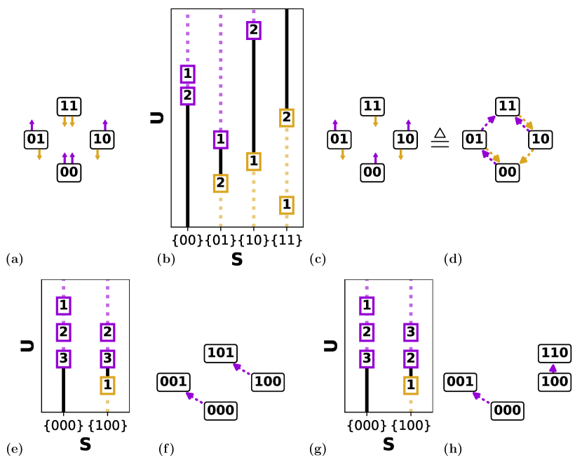
Figure 1: Scaffolds and switching fields. (a) Graphical representation of the set of $n=2$ switching fields: hysterons in state $s_{i}=0$ ($s_{i}=1$) have an up (down) switching field indicated by purple (gold) arrows. (b) Example of a given set of switching fields (boxes; number indicates hysteron index) and corresponding stability ranges (black lines) — in the dashed regions, the state is unstable. (c) Corresponding scaffold, with the $2^{n+1}-2$ critical hysterons $k^{\pm}(S)$ indicated. (d) Alternative yet equivalent graphical representation of the scaffold showing ’passages’, i.e., tentative transitions to a landing state $S^{(1)}$ that would occur upon flipping each critical hysterons $k^{\pm}(S)$ (see text). (e) Example of a subset of $n=3$ switching fields for the Preisach model where $\Delta_{i}^{\pm}(S)=0$. Since $U_{2}^{+}(000)=U_{2}^{+}(001)=u_{2}^{+}$, and $U_{3}^{+}(000)=U_{3}^{+}(001)=u_{3}^{+}$, hysterons 2 and 3 flip in the same order for both states, and since $k^{+}(000)=3$, $k^{+}(100)=3$. (f) Graphical representation of the corresponding scaffold. (g) Example of a subset of $n=3$ switching fields, for the states $\{000\}$ and $\{100\}$, for the general model where $\Delta_{i}^{\pm}(S)\neq 0$. Since the switching fields $\{U_{i}^{\pm}(S)\}$ are independent, the order in which hysterons 2 and 3 flip may be different (’scrambled’) between states $\{000\}$ and $\{100\}$. (h) Graphical representation of the corresponding scrambled scaffold.

As a first step in defining the response of a collection of hysterons to variations of the global driving field $U$, we define here the stability range of a state and its critical hysterons. We then introduce the concept of the scaffold, and use it to precisely define the concept of scrambling [5, 10, 22].

State $S$ is stable if $U$ is smaller than all its up switching fields $U_{i}^{+}(S)$ and larger than all its down switching fields $U_{i}^{-}(S)$. Hence, the stability range of $S$ is given by the state switching fields $[U^{-}(S),U^{+}(S)]$ defined as (Fig. 1b) [4]:

$$\begin{split}U^{+}(S)&=\min U_{i}^{+}(S)~{},\\ U^{-}(S)&=\max U_{i}^{-}(S)~{}.\\ \end{split}$$ (3)

When $S$ is initially stable and $U$ is swept up (down) to $U^{+}(S)$ ($U^{-}(S)$), $S$ loses stability through the instability of a single hysteron. We define these as the critical hysterons $k^{\pm}(S)$:

$$\begin{split}k^{+}(S)&=\arg\min U_{i}^{+}(S)~{},\\ k^{-}(S)&=\arg\max U_{i}^{-}(S)~{}.\\ \end{split}$$ (4)

We note here that the saturated states have only one critical hysteron, and we define $U^{-}(00\dots)=-\infty$, $U^{+}(11\dots)=\infty$. All other states have two critical hysterons and finite switching fields. We finally note that persistently unstable states may arise when $U^{+}(S)<U^{-}(S)$. Even though such states are never stable, they still can play a role as intermediate states in avalanches as we discuss in section I.2.2.

The definitions Eq. (3-4) map the $n\cdot 2^{n}$ hysteron switching fields $\{U_{i}^{\pm}(S)\}$ to $2^{n}-2$ critical hysterons $\{k^{\pm}(S)\}$, and corresponding state switching fields $\{U^{\pm}(S)\}$. We call the collection of states, critical hysterons and switching fields the scaffold, as it provides the underlying structure on which state transitions will be defined (Fig. 1c). In fact, the key role which the scaffold plays in informing the actual transitions between states motivates an alternative yet equivalent graphical representation of the scaffold: in this representation we show tentative transitions to the states that would be reached upon flipping the critical hysterons in each state. We term these tentative transitions passages. (Fig.  1d). We stress here that passages are not necessarily equal to state transitions, and we discuss the relation between scaffold and transitions in detail in section I.2.2.

The scaffold highlights that each state has at most one relevant up and down transition, and focusses on the $2^{n}-2$ state switching fields rather than the $n\cdot 2^{n}$ hysteron switching fields (compare Figs. 1a and 1c).

We now employ the scaffold to clarify the recently introduced scrambling property [5, 10, 22]. Loosely speaking, scrambling was introduced for pairs of transitions that evidence hysteron interactions [5]. However, this definition becomes complex when avalanches are present. As we show below, the scaffold allows a precise definition that does not suffer from such subtleties.

In the Preisach model, the critical hysterons for different states are tightly connected via the order of the bare hysteron switching fields $u_{i}^{\pm}$. For example, if $k^{+}(000)=2$, this implies that $u_{2}^{+}<u_{3}^{+}$, and therefore imposes that $k^{+}(100)=2$ (Fig. 1e-f). More precisely, consider two states $S_{A}$ and $S_{B}$ in the Preisach model. If the up switching hysteron in $S_{A}$ has phase 0 in $S_{B}$, and the up switching hysteron in $S_{B}$ has phase 0 in $S_{A}$, these up switching hysterons have to be equal (and similar for the down switching hysterons). Formally, if $k^{+}(S_{A})\in I_{0}(S_{B})$ and $k^{+}(S_{B})\in I_{0}(S_{A})$ then $k^{+}(S_{A})=k^{+}(S_{B})$; similarly, if $k^{-}(S_{A})\in I_{1}(S_{B})$ and $k^{-}(S_{B})\in I_{1}(S_{A})$ then $k^{-}(S_{A})=k^{-}(S_{B})$.

In contrast, for interacting hysterons the ordering of the hysteron switching fields $U_{i}^{\pm}(S)$ may be state-dependent: as an example, consider the case when $k^{+}(000)=2$ but $k^{+}(100)=3$ (Fig. 1g-h). Interactions thus lead to pairs of states with critical hysterons that cannot occur in the Preisach model: we define such pairs of states as scrambled. Formally, the critical up hysterons of a pair of states $S_{A},S_{B}$ are scrambled when $k^{+}(S_{A})\in I_{0}(S_{B})$, $k^{+}(S_{B})\in I_{0}(S_{A})$ and $k^{+}(S_{A})\neq k^{+}(S_{B})$; similarly, the critical down hysterons of $S_{A}$ and $S_{B}$ are scrambled when $k^{-}(S_{A})\in I_{1}(S_{B})$, $k^{-}(S_{B})\in I_{1}(S_{A})$ and $k^{-}(S_{A})\neq k^{-}(S_{B})$. We note that scrambling can only occur for $n\geq 3$, and define a scaffold as scrambled when it contains at least one pair of scrambled states.

I.2.2 Transitions and Avalanches

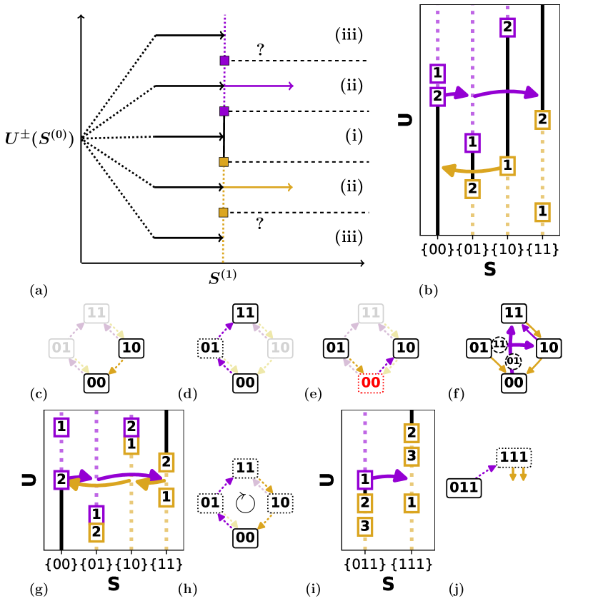
Figure 2: Construction of transitions and full transition graph from the set of switching fields. (a) Schematic of the three scenarios for the landing state $S^{(1)}$ at driving field $U^{\pm}(S^{(0)})$: (i) $S^{(1)}$ is stable; (ii) a single hysteron in state $S^{(1)}$ is unstable; (iii) $S^{(1)}$ multiple hysterons in $S^{(1)}$ are unstable (see text). (b) Two transitions ($l=1$ transition $\{10\}\rotatebox{90.0}{$\dashleftarrow$}\{00\}$ and $l=2$ transition $\{00\}\rotatebox{90.0}{$\dashrightarrow$}\{01\}\rotatebox{90.0}{$\dashrightarrow$}\{11\}$) for the set of switching fields shown in Fig. 2b. (c) The $l=1$ transition $\{10\}\rotatebox{90.0}{$\dashleftarrow$}\{00\}$ follows the scaffold (faded) (d) The avalanche transition $\{00\}\rotatebox{90.0}{$\dashrightarrow$}\{01\}\rotatebox{90.0}{$\dashrightarrow$}\{11\}$ follows the scaffold. (e) The tentative transition $\{01\}\rotatebox{90.0}{$\dashleftarrow$}\{00\}\rotatebox{90.0}{$\dashrightarrow$}\{10\}$ is incompatible with the scaffold, as the transition requires that $k^{+}(00)=1$, while the scaffold specifies that $k^{+}(00)=2$. (f) Full t-graph for the set of switching fields shown in panel b. (g) Set of switching fields that leads to a self-loop $\{00\}\rotatebox{90.0}{$\dashrightarrow$}\{01\}\rotatebox{90.0}{$\dashrightarrow$}\{11\}\rotatebox{90.0}{$\dashleftarrow$}\{10\}\rotatebox{90.0}{$\dashleftarrow$}\{00\}\rotatebox{90.0}{$\dashrightarrow$}\dots$. (h) Graphical representation for this self-loop. (i) Example of a (subset of) switching fields that leads to a race condition, due to the instability of multiple hysterons in state $\{111\}$ at $U^{+}(011)$. (j) Graphical representation for this race condition: we cannot draw a tentative down transition because the order in which hysterons 2 and 3 flip is not well defined.

When state $S$ becomes unstable, this triggers a transition to a new stable state $S^{\prime}$, which we denote as $S\rightarrow S^{\prime}$. Such a transition can be triggered by either an up sweep or down sweep of $U$, and we denote the corresponding up and down transitions as $S\uparrow S^{\prime}$ and $S\downarrow S^{\prime}$. Here we discuss in detail how the system evolves from $S$ to $S^{\prime}$, how $S^{\prime}$ is determined, and under which conditions the transition and $S^{\prime}$ are well-defined.

Each transition is initiated by the flipping of one of the critical hysterons $k^{\pm}(S)$, leading to a new ’landing’ state $S^{(1)}$. In the Preisach model, the landing state is always stable at $U_{k}^{\pm}(S)$ [20, 4, 27], so that $S^{\prime}=S^{(1)}$. This produces the transition $S\rightarrow S^{(l)}$ which trivially follows from the passages in the scaffold - in fact, for the Preisach model, transitions are equal to passages, and the scaffold captures all transitions.

In the presence of hysteron interactions, the stability of the landing state $S^{(1)}$ is no longer guaranteed, and this may lead to multi-step avalanches, which proceed via a sequence of intermediate states. We denote such transitions as $S^{(0)}\dashrightarrow S^{(1)}\dashrightarrow\dots\dashrightarrow S^{(l)}$, where $S^{(0)}$ is the initial state, $S^{(1)}$ is the landing state, $S^{(1)}-S^{(l-1)}$ are intermediate states and $S^{(l)}$ is the final state, and define the transition length as $l$.

We now show how a single transition is constructed, given the set of switching fields. A transition is initiated when $k$ flips at $U=U_{k}^{\pm}(S)$, yielding the first step $S^{(0)}\dashrightarrow S^{(1)}$. There are three possible scenarios (Fig. 2a) depending on the stability of the landing state $S^{(1)}$:

1. $S^{(1)}$ is stable at $U_{k}^{\pm}(S)$;

2. A single hysteron in state $S^{(1)}$ is unstable at $U_{k}^{\pm}(S)$;

3. Multiple hysterons in state $S^{(1)}$ are unstable at $U_{k}^{\pm}(S)$.

When the landing state $S^{(1)}$ is stable (case (i)), we obtain the $l=1$ transition $S^{(0)}\rightarrow S^{(1)}$. For example, the switching fields shown in Fig. 2b produce the $l=1$ transition $\{10\}\downarrow\{00\}$ (Fig.2b-c).

We now turn to case (ii), where a single hysteron $\kappa$ in state $S^{(1)}$ is unstable at $U=U_{k}^{\pm}(S)$. This provokes the next step $S^{(1)}\dashrightarrow S^{(2)}$ - please note that this scenario can occur even for a persistently unstable state (Section I.1). For the state $S^{(2)}$, the same three scenarios can occur as for $S^{(1)}$: if $S^{(2)}$ is stable (case (i)), the transition terminates. This produces the $l=2$ avalanche $S^{(0)}\rightarrow S^{(2)}$, which proceeds as $S^{(0)}\dashrightarrow S^{(1)}\dashrightarrow S^{(2)}$. We illustrate an example of an $l=2$ avalanche $\{00\}\rotatebox{90.0}{$\dashrightarrow$}\{01\}\rotatebox{90.0}{$\dashrightarrow$}\{11\}$ in Fig. (2b,d). If one of the hysterons in $S^{(2)}$ is unstable (case (ii)), the transition proceeds to the next state $S^{(3)}$. Assuming that case (iii) does not occur and that states are not revisited - as discussed below, both scenarios lead to ill-defined transitions[5] - we see that avalanches are constructed iteratively.

It is worth noting that all transitions must follow the passages of the scaffold. We already saw that $l=1$ transitions follow the passages, and now note that if a single hysteron $\kappa$ is unstable in the intermediate state $S^{(\lambda)}$, it must be one of the critical hysterons $k^{\pm}(S^{\lambda})$. Thus, avalanches must also follow the scaffold. Hence, once the scaffold is constructed from the switching fields, it immediately restricts the transitions that can occur; for example, for the scaffold shown in Fig. 2e, the transition $\{01\}\rotatebox{90.0}{$\dashleftarrow$}\{00\}\rotatebox{90.0}{$\dashrightarrow$}\{10\}$ is forbidden.

The relation between scaffold and avalanches can be explored to label an avalanche solely by its starting state and its sequence of up/down flips, letting the scaffold dictate the full transition path. For example, the transition path $\{00\}\rotatebox{90.0}{$\dashrightarrow$}\{01\}\rotatebox{90.0}{$\dashrightarrow$}\{11\}$ shown in Fig.  2d is labeled as 00uu. Consequently, all possible (avalanche) transitions can simply be collected in a set of binary trees; we further elaborate on and make use of this scaffold/avalanche relation in sec. III.

I.2.3 Ill-defined transitions

So far, we have discussed how a given set of switching fields produces transitions. However, there are two mechanisms by which a set of switching fields produce transitions that are ill-defined.

First, certain choices of switching fields produce self-loops, where after a number of steps, an avalanche revisits an earlier state. The simplest case is that where the switching hysteron is unstable in its landing state: for example, if after the partial transition $\{00\}\rotatebox{90.0}{$\dashrightarrow$}\{01\}$ hysteron 2 is unstable in $\{01\}$, this sets up a loop $\{00\}\rotatebox{90.0}{$\dashrightarrow$}\{01\}\rotatebox{90.0}{$\dashleftarrow$}\{00\}\rotatebox{90.0}{$\dashrightarrow$}\{01\}\rotatebox{90.0}{$\dashleftarrow$}\dots$. More generally, self-loops can arise from any cyclical path within the scaffold - for an example of a longer loop, see Fig. 2g-h. Such an orbit can never reach a stable state, and as hysteron systems are dissipative, such loops cannot occur in physical systems. We consider the hysteron model ill-defined for switching fields that produce such self-loops[5].

Second, when a transition reaches an intermediate state $S^{(\lambda)}$ where more than one hysteron is unstable at the critical field $U^{\pm}(S^{(0)})$, we consider the transition ill-defined - for an example of such case (iii) scenario, see Fig. 2i-j. The problem is that when multiple hysterons are unstable, the sequence of hysteron flips is ill-defined thus setting up a race condition [28]. As the hysterons are interacting, flipping operations do not commute: for example, when the hysterons $\kappa_{1}$ and $\kappa_{2}$ are unstable, and hysteron $\kappa_{1}$ flips first, this may make hysteron $\kappa_{2}$ stable again, whereas when hysteron $\kappa_{2}$ flips first, hysteron $k_{1}$ may remain unstable. Hence, different choices for the sequence of hysteron flips may then lead to different transition paths, a situation known as a critical race condition [28]. Such transition paths may break away from the scaffold, resulting in graphs that would not otherwise be possible. We note that some authors resolve race conditions by simply demanding that each intermediate step in a transition only flips one hysteron, and picking the most unstable hysteron if there is more than one; for such a model, the scaffold/avalanche relation is maintained [6, 7].

Both self-loops and race conditions arise because models for interacting hysterons have a very simple update rule. More physically complete models, based on an energy landscape and a dynamical rule, would not feature race conditions or loops — transitions would be well defined and loops would be avoided due to dissipation. All in all, hysteron models are perhaps the alpha, but not the omega of studies of the sequential response of complex media. Nevertheless, studies of more complex models come at a significant computational expense, and despite their (over)simplicity, hysteron models have proven valuable in capturing experimental and numerical data, as well as giving insight in memory effects.

I.3 Transition Graphs

All ingredients are now in place to construct the transition graph (t-graph) which encodes the full driving response for a set of hysteron switching fields $U_{i}^{\pm}(S)$. To do so, we first construct the scaffold (Section I.2.1), and then iteratively construct the full transition path $S^{(0)}\dashrightarrow S^{(1)}\dashrightarrow\dots\dashrightarrow S^{(l)}$ for each up and down transition. We collect these transitions in a directed graph, where the states form the nodes, and the transitions $S^{(0)}\rightarrow S^{(l)}$ form the edges. Each edge has further attributes: the value of the critical switching field, the direction (up/down), and the intermediate states $S^{(1)},\dots,S^{(l-1)}$. For example, the set of switching fields $\{U_{i}^{\pm}(S)\}$ shown in Fig. 2b produces a well-defined t-graph (Fig. 2f). In summary, the driving response of a collection of $n$ hysterons, characterized by a set of switching fields $\{U_{i}^{\pm}\}$, is captured by a directed t-graph.

We note that our t-graphs contain more information than what is usually considered. First, for a given set of switching fields the intermediate states are fully specified, whereas in, e.g., experimental contexts intermediate states in an avalanche can typically not be observed [10]. Second, our t-graphs may contain so-called Garden-of-Eden (GoE) states that are not reachable from the saturated states (for an example see state $\{01\}$ in Fig. 2f) [5, 11]. Unless otherwise specified, we will deal with t-graphs where GoE states and intermediate states are both included. In our visualization of t-graphs, we thus not only indicate a transition’s direction (up/down) and length $l$[5] but also explicitly indicate the intermediate states.

II Graph Design

In this section we consider the design question, also referred to as the inverse problem: given a transition graph, or part of a transition graph, what are the necessary and sufficient conditions on the switching fields so that they lead to this (sub)graph? Consistent with earlier work on this inverse problem [5, 7], we find that the design conditions take the form of sets of inequalities of the switching fields. Here, we establish a systematic approach for constructing and utilizing these design inequalities. We first present their systematic derivation (section II.1), then discuss how the design inequalities specify a partial order on the switching fields (section II.2). In particular, we utilize the inequalities to determine if a given t-graph topology is realizable (section II.2.2), and finally discuss how to construct explicit sets of switching fields that realize specific (sub)-graphs (section II.2.3).

II.1 Design Inequalities

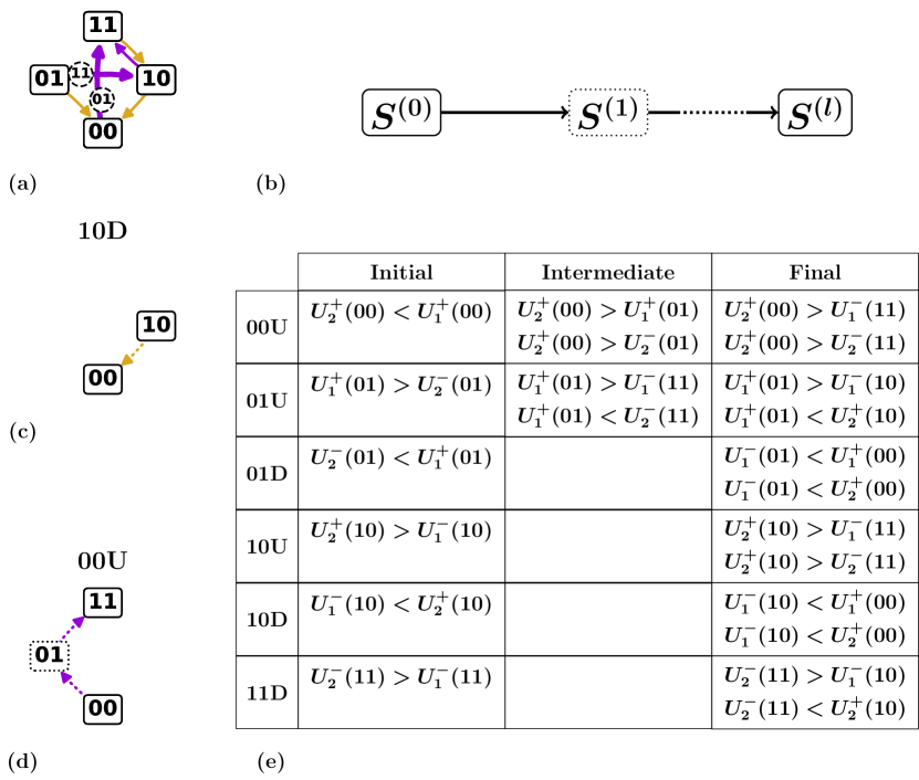
Figure 3: Design inequalities. (a) Example of an $n=2$ target t-graph. (b) The design inequalities are organized in three groups pertaining to the initial state $S^{(0)}$, intermediate states $S^{(1)},\dots,S^{(l-1)}$, and final state $S^{(l)}$. (c) Length-1 transition $\{10\}\rotatebox{90.0}{$\dashleftarrow$}\{00\}$. (d) Length-2 transition $\{00\}\rotatebox{90.0}{$\dashrightarrow$}\{01\}\rotatebox{90.0}{$\dashrightarrow$}\{11\}$. (e) The design inequalities for the target graph shown in panel (a). We label transitions by their starting state $S^{(0)}$ and their up or down direction: for example, the up transition starting from state $\{00\}$ is labeled 00U, and the down transition starting from state $\{10\}$ is denoted 10D (see also panels (c) and (d)). Note that all inequalities are organized by transition, and can be further separated by whether they are given by the initial state (scaffold), intermediate state (if present), or final state inequalities.

We define the design inequalities as the necessary and sufficient conditions on the switching fields $\{U_{i}^{\pm}(S)\}$ that produce a specific (sub)graph. We will frequently illustrate our approach with specific examples, such as the t-graph and its scaffold shown in Fig. 3a. As we show, each transition in a t-graph corresponds to a set of design inequalities that result from (i) conditions on the initial state (its stability and critical hysterons) (ii) the stability of the final state, and, if the transition is an avalanche, (iii) the (in)stabilities and critical hysterons of the intermediate states (section II.1.1). Combining the individual design inequalities for multiple transitions, taking potential redundancies into account, produces the set of inequalities for a specific t-graph or part thereof.

II.1.1 Conditions for Single Transitions

We now derive the design inequalities for a single transition. As avalanches for which only the initial state $S^{(0)}$ and final state $S^{(l))}$ are specified may proceed along various paths of intermediate states, each producing a different set of design inequalities, we assume that the full transition path $S^{(0)}\dashrightarrow S^{(1)}\dashrightarrow\dots\dashrightarrow S^{(l))}$ is known (Fig. 3b).

Initial inequalities.

The first set of design inequalities follows from the required stability of state $S^{(0)}$ for some range of $U$, and from the critical hysteron $k$ that flips when the driving $U$ is increased or decreased.

The first step in the transition $S^{(0)}\dashrightarrow S^{(1)}$ specifies that hysteron $k$ in state $S^{(0)}$ becomes unstable when $U$ is increased (decreased). This requirement leads to a set of inequalities which specifies that the corresponding up (down) switching field $U_{k}^{\pm}(S^{(0)})$ must be the lowest (highest) of all up (down) switching fields at this state:

up: $$U_{k}^{+}(S^{(0)})<U_{i}^{+}(S^{(0)}) \mbox{ $\forall i\in I_{0}(S^{(0)})\backslash\{k\}$}~{},$$ (5)

down: $$U_{k}^{-}(S^{(0)})>U_{i}^{-}(S^{(0)}) \mbox{ $\forall i\in I_{1}(S^{(0)})\backslash\{k\}$}~{}.$$ (6)

Here $I_{0/1}(S^{(0)})\backslash\{k\}$ is the collection of hysterons in phase $0~{}(1)$, unequal to $k$ in state $S^{(0)}$.

Moreover, state $S^{(0)}$ must be initially stable, and for an up (down) transition, this requires all down (up) switching fields to be below (above) the critical switching field $U_{k}^{\pm}(S^{(0)})$:

up: $$U_{k}^{+}(S^{(0)})>U_{i}^{-}(S^{(0)}) \mbox{ $\forall i\in I_{1}(S^{(0)})$}~{},$$ (7)

down: $$U_{k}^{-}(S^{(0)})<U_{i}^{+}(S^{(0)}) \mbox{ $\forall i\in I_{0}(S^{(0)})$}~{},$$ (8)

We illustrate the initial state inequalities using the example t-graph shown in Fig. 3a. The condition for the up transition from state $\{00\}$ to be initiated by critical hysteron $k^{+}(00)=2$ is $U_{2}^{+}(00)<U_{1}^{+}(00)$, and the stability condition is trivially satisfied. Similarly, the down transition from state $\{11\}$ produces one critical hysteron condition and no stability conditions. In contrast, the up and down transitions from the states $\{01\}$ and $\{10\}$ specify one stability condition and no conditions for the critical hysterons. In general, there are $n-1$ initial state inequalities, which arise from the comparison of the critical hysteron $k$ against every other hysteron.

Final Inequalities.

For each transition, the final state $S^{(l)}$ needs to be stable at the critical driving $U_{k}^{\pm}(S)$ where the transition is initiated. This requirement produces inequalities of the form:

$$U_{k}^{\pm}(S)<U_{i}^{+}(S^{(l)}) \mbox{ $\forall i\in I_{0}(S^{(l)})$}~{},$$ (9)

$$U_{k}^{\pm}(S)>U_{i}^{-}(S^{(l)}) \mbox{ $\forall i\in I_{1}(S^{(l)})$}~{},$$ (10)

For example, for the transition $\{10\}\downarrow\{00\}$ (Fig. 3c), the stability of the final state $\{00\}$ at $U_{1}^{-}(10)$ yields:

$$U_{1}^{-}(10) < U_{1}^{+}(00)~{},$$ (11)

$$U_{1}^{-}(10) < U_{2}^{+}(00)~{}.$$ (12)

In general, as each hysteron in state $S^{(l)}$ needs to be stable under the critical field $U_{k}^{\pm}(S)$, each transition produces $n$ final state inequalities.

Intermediate Inequalities.

While $l=1$ transitions, like $\{10\}\rotatebox{90.0}{$\dashleftarrow$}\{00\}$ in the example of Fig. 3, only produce initial state and final state inequalities, each intermediate step in an avalanche of length $l>1$ produces additional conditions to ensure that each intermediate step is well-defined and proceeds as described.

As an example, consider an avalanche initiated at $U=U_{k}^{\pm}(S)$ and an intermediate state $S^{(\lambda)}$ where hysteron $\kappa$ switches up, so $\kappa=k^{+}(S^{(\lambda)})$. The requirement that hysteron $\kappa$ is unstable at $U_{k}^{\pm}(S)$, while all other hysterons are stable, leads to the intermediate state inequalities:

$$U_{k}^{\pm}(S) <U^{+}_{i}(S^{(\lambda)}) \mbox{ $\forall i\in I_{0}(S^{(\lambda)})\backslash\{\kappa\}$}~{},$$ (13)

$$U_{k}^{\pm}(S) >U_{i}^{-}(S^{(\lambda)}) \mbox{ $\forall i\in I_{1}(S^{(\lambda)})$}~{},$$ (14)

$$U_{k}^{\pm}(S) >U_{\kappa}^{+}(S^{(\lambda)}) ~{}.$$ (15)

Similarly, when hysteron $\kappa$ switches down, the first two equations remain the same, but the last one changes to $U_{k}^{\pm}(S)<U_{\kappa}^{-}(S^{(\lambda)})$.

As an example, consider the $l=2$ avalanche $\{00\}\rotatebox{90.0}{$\dashrightarrow$}\{01\}\rotatebox{90.0}{$\dashrightarrow$}\{11\}$(Fig. 3d). The instability of hysteron 1 at the intermediate state $\{01\}$ gives rise to the equations:

$$U_{2}^{+}(00) > U_{1}^{+}(01)~{},$$ (16)

$$U_{2}^{+}(00) > U_{2}^{-}(01)~{}.$$ (17)

We note that, like for the final inequalities, there are $n$ intermediate inequalities for each of the states $S^{(1)},\dots,S^{(l-1)}$, which specify the stability of each hysteron in $S^{(\lambda)}$ under $U_{k}^{\pm}(S)$.

II.1.2 Full Graph

Combining the initial, intermediate and final inequalities, one obtains a set of inequalities that the switching fields must obey so that a given transition is realized. We see that, for example, the transition $\{00\}\rotatebox{90.0}{$\dashrightarrow$}\{01\}\rotatebox{90.0}{$\dashrightarrow$}\{11\}$ requires five inequalities: one initial inequality, two intermediate inequalities, and two final inequalities. In general, the number of inequalities per transition is $(l+1)n-1$.

This approach constructs conditions on the level of individual transitions, and is therefore modular. To construct design inequalities for t-graphs or subgraphs thereof, we simply combine the conditions of their respective transitions. We note that there are often redundancies between these inequalities: for example, in Figure 3f, the inequality $U_{1}^{+}(00)>U_{2}^{-}(10)$ appears twice.

II.2 Partial order and matrix representation

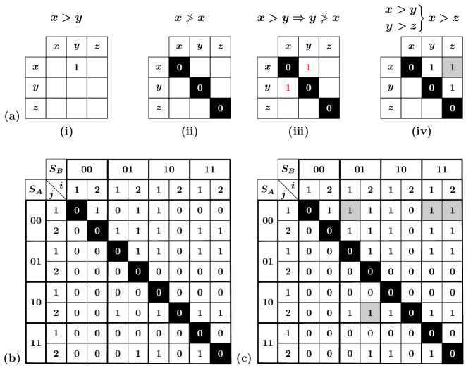
Figure 4: Partial order represented by adjacency matrices. (a) Representation of a partial order as an adjacency matrix (i) and three properties of a partial order: (ii) irreflexivity, shown by the diagonal highlighted in white-on-black; (iii) asymmetry, shown by a pair of entries highlighted in red, where $x>y$ rules out that $y>x$; and (iv) transitivity, where the induced inequality $x>z$ is highlighted in gray. (b) Example of the list of design inequalities shown in Fig. 3e as the adjacency matrix $P$. The matrix contains $n\times n$ blocks of inequalities that concern the same states $S_{A},S_{B}$, as shown by thicker lines. Notably, the block diagonal consists of the initial inequalities, as they concern comparisons between switching fields at the same state. (c) Transitive closure $P^{*}$ of the adjacency matrix $P$ shown in (b); note the addition of induced inequalities, highlighted in gray.

The design inequalities specify a partial order on the switching fields $U_{i}^{\pm}(S_{j})$. To see this, note that the design inequalities are a collection of pairwise inequalities of the form $U_{i}^{\pm}(S_{A})>U_{j}^{\pm}(S_{B})$. Crucially, whereas any ordering of the switching fields maps to a single t-graph topology, the converse is not true: a given topology may be consistent with multiple orderings. As we will see, there are also ’forbidden’ t-graph topologies for which no consistent order can be constructed.

We note that this situation, where the mapping from ordering to t-graph is injective but not invertible, generalizes the situation in the Preisach model. There the graphs are uniquely determined by the orderings of the up switching fields and those of the down switching fields; the order of pairs of one up and one down switching field does not play a role, except for the constraint that $u_{i}^{+}>u_{i}^{-}$ [20, 27]. Hence, in the Preisach model, the ordering of the state-independent switching fields $u_{i}^{\pm}$ also uniquely determines the t-graph topology but not vice versa.

In this section, we consider the fundamental role of the ordering of the switching fields. We first present a graphical representation and method to construct the partial order (section II.2.1). Second, while any target t-graph can be mapped to a set of design inequalities, the converse is not true: some target t-graph topologies are simply not consistent with any set of switching fields. For such a case, the corresponding design inequalities show up as violations of asymmetry — i.e., $x>y$ and $x<y$ — and this allows to systematically and quickly check if a given t-graph topology is realizable (section II.2.2). Finally, if the design inequalities are solvable, we discuss how one can compute specific examples of switching fields consistent for a given t-graph (section II.2.3).

II.2.1 Constructing a partial order

We represent the partial order of the switching fields via an adjacency matrix $P$, where a 1 at position $(x,y)$ indicates the presence of a design inequality $x>y$, and a 0 indicates no relation (Fig. 4a-(i)). It is useful at this point to recall the general properties of partial orders — irreflexivity, asymmetry, and transitivity — and translate these properties to the adjacency matrix $P$. First, irreflexivity entails that $x\ngtr x$, so that all diagonal elements of $P$ are zero (Fig. 4a-(ii)). Second, a partial order relation is asymmetric, such that if $x>y$, then $y\ngtr x$. In the matrix representation, this means a 1 at position $(x,y)$ rules out a 1 at position $(y,x)$ and vice versa (Fig. 4a-(iii)). Hence, as we discuss below, if the design inequalities would specify such a pair, they do not have a solution. Finally, a partial order has transitivity, meaning that if $x>y$ and $y>z$, then $x>z$ (Fig. 4a-(iv)). Including all such induced inequalities yields the transitive closure [29], and we define the corresponding transitive closure matrix $P^{*}$. Note that, while different matrices $P$ may imply the same partial order relation, the transitive closure for a given partial order is unique [29]. Therefore, it is the transitive closure matrix $P^{*}$ that corresponds one-on-one to a t-graph.

We now illustrate the construction of $P$ and $P^{*}$ for the design inequalities tabulated in Fig. 3f. The rows and columns of the partial order matrix $P$ correspond to the $n\cdot 2^{n}$ switching fields $U_{i}^{\pm}(S)$. We index the entry of the matrix corresponding to a pair of switching fields $U_{i}^{\pm}(S_{A})$, $U_{j}^{\pm}(S_{B})$ as $(S_{A},i;S_{B},j)$. By placing a 1 at any positions $(S_{A},i;S_{B},j)$ where one has a relation $U_{i}^{\pm}(S_{A})>U_{j}^{\pm}(S_{B})$, and a 0 elsewhere, one obtains the adjacency matrix representation $P$ of the design inequalities (Fig. 4b). We note that, whereas there are 19 design inequalities, $P$ only features 17 entries ’1’, because two inequalities appear twice (see Fig. 3). Based on $P$, we use a transitive closure algorithm such as Warshall’s algorithm [30] to uniquely construct the matrix $P^{*}$ (Fig. 4c). Hence, given any t-graph, the construction of the partial order $P^{*}$ is straightforward.

II.2.2 Realizability of t-graphs

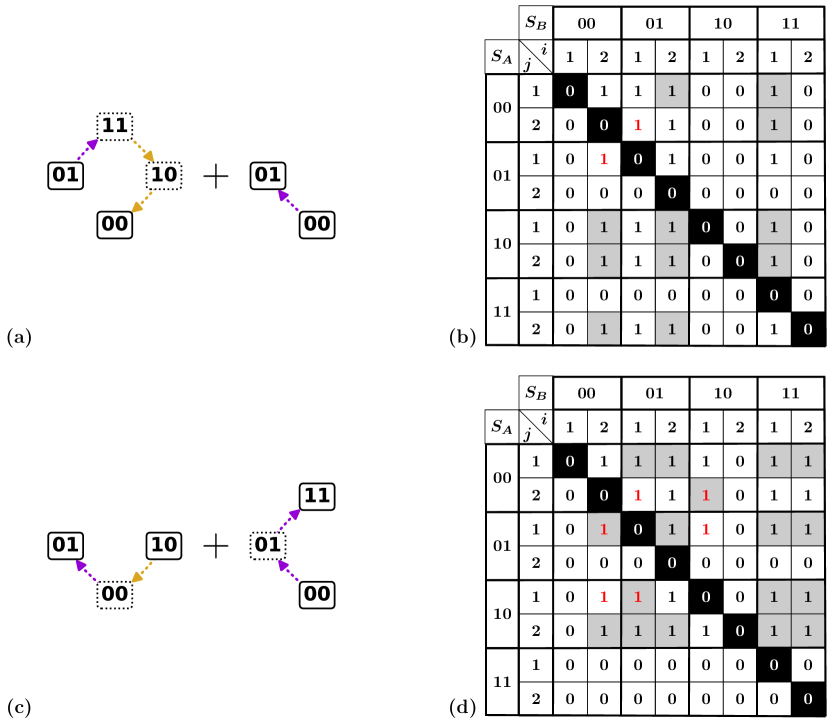
Figure 5: Illustration of impossible subgraphs and corresponding design inequalities. (a) Tentative combination of transitions $00\rotatebox{90.0}{$\dashrightarrow$}01$ and $01\rotatebox{90.0}{$\dashrightarrow$}11\rotatebox{90.0}{$\dashleftarrow$}10\rotatebox{90.0}{$\dashleftarrow$}00$. (b) Corresponding design inequalities $P^{*}$, with entries induced via transitivity highlighted in gray. The entries (00, 2; 01, 1) and (01, 1; 00, 2) show that asymmetry is broken (highlighted in red); note that the contradictory pair of inequalities already appears in the original set of inequalities $P$ (white blocks). (c) Tentative subgraph containing transitions $00\rotatebox{90.0}{$\dashrightarrow$}01\rotatebox{90.0}{$\dashrightarrow$}11$ and $10\rotatebox{90.0}{$\dashleftarrow$}00\rotatebox{90.0}{$\dashrightarrow$}01$. (d) Corresponding design inequalities $P^{*}$. The three pairs of entries highlighted in red show that the asymmetry condition is broken; note that this breaking of asymmetry is only visible in the transitive closure $P^{*}$, and not in the original matrix $P$.

While any target t-graph can be mapped to a set of design inequalities, design inequalities may at times contradict each other, such that they are not consistent with any set of switching fields. Hence, the question of existence of a set of switching fields that realize a target t-graph is tantamount to checking the satisfiability of the set of design inequalities. To solve the general problem of checking whether a set of inequalities is consistent, one can use the classical method of Fourier-Motzkin elimination [31], or alternatively, more refined linear programming methods such as the simplex algorithm [32].

For our sets of pairwise inequalities, checking solvability is more straightforward than in the general case: inconsistencies show up as violations of asymmetry, i.e., pairs of inconsistent inequalities of the form $x>y$ and $x<y$ occurring simultaneously. These pairs are easily detected using the matrices $P$ and $P^{*}$ introduced above. We illustrate our approach by discussing two examples of non-realizable t-graphs.

First we consider a target t-graph that contains a subgraph consisting of the $l=1$ up transition $\{00\}\rotatebox{90.0}{$\dashrightarrow$}\{01\}$, and the $l=3$ up transition $\{01\}\rotatebox{90.0}{$\dashrightarrow$}\{11\}\rotatebox{90.0}{$\dashleftarrow$}\{10\}\rotatebox{90.0}{$\dashleftarrow$}\{00\}$ (Fig. 5a). For this example a contradiction in the design inequalities is immediately visible from the partial order matrix $P$: the stability of the final state $\{01\}$ of the transition $\{00\}\rotatebox{90.0}{$\dashrightarrow$}\{01\}$ requires $U_{2}^{+}(00)<U_{1}^{+}(01)$, while the stability of the final state $00$ of the transition $\{01\}\rotatebox{90.0}{$\dashrightarrow$}\{11\}\rotatebox{90.0}{$\dashleftarrow$}\{10\}\rotatebox{90.0}{$\dashleftarrow$}\{00\}$ requires $U_{2}^{+}(00)>U_{1}^{+}(01)$. This contradiction is directly visible in $P$, as the symmetry related entries $(00,2;01,1)$ and $(01,1;00,2)$ both are 1, which is forbidden (Fig. 5b). Hence, the stability conditions directly produce a pair of inconsistent inequalities, and the target graph can not be realized within a model of interacting hysterons.

Second, we consider Fig. 5c. For this example the contradiction in the design inequalities is not directly visible in $P$, and requires the construction of $P^{*}$. To see this, note that the up transition $\{00\}\rotatebox{90.0}{$\dashrightarrow$}\{01\}\rotatebox{90.0}{$\dashrightarrow$}\{11\}$ requires that $U_{2}^{+}(00)>U_{1}^{+}(01)$, while the down transition $\{01\}\rotatebox{90.0}{$\dashleftarrow$}\{00\}\rotatebox{90.0}{$\dashrightarrow$}\{10\}$ requires $U_{1}^{+}(01)>U_{2}^{-}(10)$ and $U_{1}^{-}(10)>U_{2}^{+}(00)$. Together, this leads to the inconsistent chain of inequalities $U_{2}^{+}(00)>U_{1}^{+}(01)>U_{2}^{-}(10)>U_{2}^{+}(00)$ which cannot be identified immediately from $P$, but when we construct the transitive closure $P^{*}$, such contradictions become manifest (Fig. 5d). Hence, this target graph can not be realized.

II.2.3 Solving the design inequalities

To conclude, we discuss how explicit solutions for the switching fields $\{U_{i}^{\pm}(S)\}$ can be constructed for a given set of (consistent) design inequalities. For our sets of pairwise inequalities, an explicit solution can be constructed by finding a total order (or ’linear extension’ [22]) that satisfies the partial order specified by the design inequalities. We use a topological sorting algorithm such as Kahn’s algorithm[33, 34] to produce a random linear extension, without regard for the range and distributions of gaps between switching fields.

To convert such a random linear extension to an explicit solution, we set the switching fields to be equidistant with a spacing of $\epsilon={\left(n\cdot 2^{n}\right)}^{-1}$, and set the lowest switching field to $\epsilon/2$. This is a convenient choice because it guarantees that the switching fields lie within the range $[0,1]$, and the system is in the saturated states $\{00...\}$, $\{11...\}$ at driving values of 0 and 1 respectively.

Although we have emphasized that the design inequalities for a given t-graph topology only impose a partial order relation, additional constraints - for example, those imposed by the use of a specific model for $\Delta_{i}^{\pm}(S)$ - can lead to more complex sets of inequalities. In these cases, one can fall back on general linear programming methods such as the simplex algorithm [32] to solve the full set of inequalities. We note that, to make use of linear programming, one must first transform the set of strict design inequalities to a set of non-strict design inequalities $U_{i}^{\pm}(S_{A})-U_{j}^{\pm}(S_{B})\geq b$, with $b$ a small positive number. Like $\epsilon$ in the method described above, $b$ here sets an explicit spacing between switching fields, which is necessary because the problem is scale-invariant otherwise.

Altogether we have shown how for any t-graph or subgraph, we can construct corresponding design inequalities. These design inequalities allow us to check if a t-graph is realizable and, if so, to generate a random set of switching fields that realizes the graph. We make use of this in section III to generate all valid t-graphs for $n=2$. Moreover, the process of checking solvability and finding a solution is facilitated by the observation that the design inequalities only specify a partial order on the switching fields (section II.2). This observation has further implications for the statistical weight of t-graphs, as we will discuss in section IV.

III Constructing and organizing all graphs

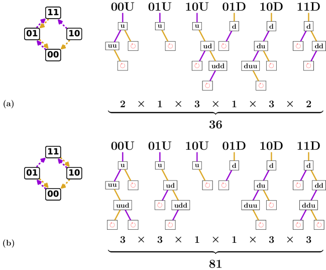
Figure 6: Binary trees of possible avalanches for $n=2$. a) First of two possible scaffolds for $n=2$, and associated binary trees of avalanches per transition. We label transitions by their starting state $S^{(0)}$ and their up or down direction marked respectively as U or D (see also Fig.3). Each tree node represents a transition $S^{(0)}\rightarrow\dots\rightarrow S^{(l)}$, characterized by a starting state and up/down sequence - please note the difference between uppercase and lowercase labels, as U and D signify the initial direction of a transition, whereas u and d signify intermediate steps. A length-$l$ transition can be extended to a transition of length $l+1$ by an up flip if $S^{(l)}=\{00...\}$, by a down flip if $S^{(l)}=\{11...\}$, and by either an up or down flip otherwise. Branches of the tree terminate where there is a self-loop, indicated in red. The number of avalanches in each tree is indicated below each transition; the product of these counts gives the number of avalanches for the given scaffold. b) Second of two possible scaffolds for $n=2$, and associated binary trees of avalanches per transition. Note that the structure of each tree is as in (a), but the nodes at which self-loops are encountered are different.

In this section we consider the space of all t-graphs. While the profusion of t-graphs with $n\geq 3$ makes brute force explorations unfeasible [5], we build here on the observation that any t-graph is created by combining transitions which proceed on a scaffold (sections  I.2.1, I.3). Thus, to systematically explore the space of all t-graphs, we proceed in three steps. First, for given $n$, we create and count all scaffolds (section III.1). Second, for any state in a scaffold, all possible (avalanche) transitions can be organized by finite binary trees (section III.2). Third, by combining scaffolds and selecting transitions from the binary trees, all candidate t-graphs can be systematically generated. Only a fraction of these are consistent with the corresponding design inequalities, and these are the sought-after valid t-graphs. We use this approach to determine all valid t-graphs for $n=2$, all scaffolds (and all avalanche-free t-graphs) for $n=3$, and a loose upper bound on the number of t-graphs for $n=3$ (section III.3). Our approach uncovers the root cause of the multiplicity and complexity of the space of all t-graphs: as each state allows a number of potential transitions, the multiplication of these numbers very quickly leads to astronomical numbers, while at the same time, the combination of longer and longer avalanches eventually leads to many t-graphs of which the design inequalities are inconsistent. Thus, while the number of valid t-graphs for general $n$ is presumably much smaller than the number of candidate graphs, the complexity of the underlying design inequalities makes it challenging to systematically construct - or even enumerate - these graphs.

III.1 Scaffolds

We now consider the multiplicity and organization of the scaffolds. We first define the up (down) boundary of a scaffold as the sequences of up (down) passages that connect the saturated states $\{00\dots\}$ and $\{11\dots\}$; together these form the main loop [20, 27]. We break the relabeling symmetry of the hysterons by requiring that the sequence of passages that connects the up boundary of the main loop is fixed, so that the hysterons flip in the order $n,n-1,\dots,1$ [20]. With this convention, there are $n!$ possible down boundaries and hence $n!$ main loops, which can be labeled by the sequence of down transitions. For example, the main loop of the scaffold in Fig. 6a, $\{00\}\rotatebox{90.0}{$\dashrightarrow$}\{01\}\rotatebox{90.0}{$\dashrightarrow$}\{11\}\rotatebox{90.0}{$\dashleftarrow$}\{01\}\rotatebox{90.0}{$\dashleftarrow$}\{00\}$, can be denoted as $(1,2)$ [20, 27].

The number $N_{s}(n)$ of scaffolds for $n$ hysterons can be obtained from a simple combinatorial argument. For each up (down) transition, the number of possible critical hysterons $n^{\pm}(S)$ equals the number of hysterons in phase 0 (1), so that $n^{+}(S)=n-m$ and $n^{-}(S)=m$, where $m$ denotes the magnetisation which follows from $S$ straightforwardly. As the number of states with magnetisation $m$ equals $\binom{n}{m}$, we immediately find that

$$N_{S}=\frac{\prod_{S}(n^{+}(S)~{}n^{-}(S))}{n!}=\frac{{\left(\prod_{m=1}^{n}m^{\binom{n}{m}}\right)}^{2}}{n!}~{},$$ (18)

where the division by $n!$ takes care of the relabeling symmetry.

The scaffolds can simply be labeled by the values of the critical hysterons, and can be organized by main loop and by the minimal number of scrambled passages. First, each main loop allows for the same number of scaffolds ($N_{S}/n!$) — to see this, note that, irrespective of the main loop, the same amount of choices of up and down transitions at each value of $m$ are available. Second, for each main loop we can define one unscrambled or Preisach scaffold, where all critical transitions follow the order of the up and down transitions along the main loop; all other scaffolds are obtained by scrambling, i.e. changing one or more critical hysterons. This suggests that we can characterize the complexity of the scaffold by the minimal number of such changes.

The scaffolds are far less numerous than t-graphs. For example, for $n=3$, there are only 96 scaffolds in total, and sixteen scaffolds per main loop. For $n=2$ we see that $N_{S}=2$, and so there is only a single scaffold per main loop; this reaffirms that scrambling can only occur for $n>2$. Because they are less numerous, scaffolds facilitate exploration of t-graphs.

III.2 Binary trees of transitions

We now discuss how, for a given scaffold, all (avalanche) transitions starting at a given state $S$ and initial direction can be organized in a finite binary tree (Fig. 6). To construct this tree, we start from a state and initial direction, and then iteratively construct all sequences of up and down steps in the scaffold (recall that only one hysteron can flip phase at each step in an avalanche). Since the number of hysterons is finite, the magnetization spans a finite range, so we terminate all branches that attempt an up (down) step from the saturated state $\{11\dots\}~{}(\{00\dots\})$. Furthermore, since each avalanche may visit states only once due to the ’no-loop’ condition, we also terminate branches that revisit a state. Hence, all branches in this tree terminate after a finite number of steps.

As an example, we consider the $n=2$ scaffold with down boundary (1, 2), and focus on the up transitions starting from $\{00\}$ (Fig. 6a). First, we construct the $l=1$ transition 00u - note the scaffold stipulates that $k^{+}(S)=2$, so that 00u corresponds to the transition $\{00\}\rotatebox{90.0}{$\dashrightarrow$}\{01\}$. We now check if the $l=2$ extensions of this transition, 00uu and 00ud, are allowed. Using the scaffold, we find that 00uu corresponds to the valid transition $\{00\}\rotatebox{90.0}{$\dashrightarrow$}\{01\}\rotatebox{90.0}{$\dashrightarrow$}\{11\}$, whereas 00ud leads to a self-loop and is forbidden; we terminate this branch (Fig. 6a). Extending 00uu, we find that 00uuu (not drawn) does not exist as there are no hysterons to flip up, and 00uud leads to a self-loop. All branches have now terminated, so we find that the only valid up sequences for transition 00U are 00u and 00uu. Repeating this procedure for all states and initial directions, we can construct six binary trees for this example scaffold containing twelve potential transitions in total(Fig. 6a). For $n=2$ there are only two scaffolds, and for the second scaffold we can construct fourteen potential transitions (Fig. 6b).

III.3 Constructing all t-graphs

By combining scaffolds and selecting (avalanche) transitions from the corresponding binary trees, we can systematically generate all so-called candidate t-graphs; if the corresponding design inequalities are consistent, such candidate graphs are valid t-graphs (section II.2.2).

For the $n=2$ case, by multiplying the sizes of all binary trees of transitions, we find that the first scaffold yields $2\times 1\times 3\times 1\times 3\times 2=36$ candidate graphs (Fig. 6a), while the second scaffold yields $81$ candidate graphs (Fig. 6b), yielding a total of 117 $n=2$ candidate graphs. We observe that the list of candidate graphs is often dominated by a single or small set of scaffold(s), due to the combinatorial explosion associated with large trees.

To determine all valid t-graphs, we simply check for each candidate graph whether it is realizable (section II.2.2). For $n=2$, we find that 35 of the 117 candidate graphs are realizable. When we exclude Garden-of-Eden states from the graph topology (section I.3) this number reduces to only thirteen. When we ignore the intermediate states of the avalanches, the number reduces further to eleven. All of these graphs were found previously using sampling [5]; we can now state conclusively that these are the only possible graphs for $n=2$ interacting hysterons.

The number of candidate graphs to be checked increases very rapidly with the number of hysterons. For just $n=3$ hysterons, we can systematically construct all trees for each of the 96 possible scaffolds, obtain all candidate graphs by multiplying the sizes of these trees for each scaffold, and then sum over the scaffolds; doing so, we obtain 4725217377852 candidate graphs. All of these candidate graphs need to be individually checked for realizability; thus, it is not feasible to use this method to find all realizable t-graphs for more than two interacting hysterons.

However, the enumeration of scaffolds and trees allows to gain insight into the space of possible t-graphs. For example, the 96 scaffolds for $n=3$ produce exactly 96 avalanche-free t-graphs When GoE states are excluded, this number even reduces further to 35. We note in passing that a total order of the state switching fields can easily be constructed such that an avalanche-free t-graph is obtained, for any choice of the scaffold. For example, one can use a ’staircase’ construction, where one first orders the state switching fields according to magnetization as $U^{-}(m=1)<U^{+}(m=0)<U^{-}(m=2)<U^{+}(m=1)<U^{-}(m=3)\dots$, and then arbitrarily choose an order of the state switching fields at each magnetization to obtain a well defined total order. By substituting these state switching fields $U^{\pm}(S)$ for the appropriate hysteron switching fields $U_{i}^{\pm}(S)$, one can obtain a total order that produces an avalanche-free t-graph for any scaffold. Thus, all 96 avalanche-free candidate graphs for $n=3$ (or 35 when excluding GoE states) are valid t-graphs.

We now illustrate how one can use the binary tree structure to include avalanches step by step. Considering again the $n=2$ transitions in Fig. 6, we first focus on only the $l=2$ avalanches. We see that there are four of these $l=2$ avalanches per scaffold. For the scaffold with main loop (1, 2), the corresponding sequences are 00uu, 10ud, 10du and 11dd - the sequences 00ud, 01du are forbidden because of self-loops. Similarly, the scaffold with main loop (2, 1) allows for four $l=2$ transitions 00uu, 01ud, 10du and 11dd. Thus, in total, we can construct eight candidate graphs with only a single $l=2$ avalanche. We find that all these candidate graphs are realizable.

We can apply the same approach for $n=3$. Considering the binary trees of transitions for each of the 96 scaffolds, we find that each of the scaffolds allows for either fourteen, sixteen or eighteen possible $l=2$ transitions - as we saw for $n=2$, this number depends on the number of $l=2$ transitions that lead to self-loops, and because these transitions must come in pairs, the total number of $l=2$ transitions is even. Summing over all scaffolds, we find that there are 1440 candidate graphs with a single $l=2$ transition. Again checking for each of these candidate graphs whether the design inequalities are consistent, we find that all these graphs are realizable. We believe that this phenomenon - where all candidate graphs with a single $l=2$ avalanche are realizable - extends to general $n$. To see that all such graphs are realizable, we need to construct a consistent order for the switching fields. To do so, one starts from a ’staircase’ construction to create a total order for the t-graph without avalanches, and then only modifies the switching fields responsible for the avalanche, leading to a minor change in the ordering.

For the next step in complexity, we have two options: we can either consider t-graphs with a single $l=3$ avalanche, or t-graphs which have two $l=2$ avalanches. We note that whereas candidate graphs with a single $l=2$ avalanche appear to always be realizable, neither candidate graphs with a single $l=3$ avalanche nor those with two $l=2$ avalanches are necessarily realizable, as can be seen from the example subgraphs in Figure 5.

We first consider the case of a single $l=3$ avalanche, once again starting with the simple $n=2$ case shown in Fig. 6. Like in the $l=2$ case, we can simply count the number of $l=3$ transitions in Fig. 6 to find that the scaffold with main loop (1, 2) has two possible $l=3$ transitions (10udd and 10duu) and the scaffold with main loop (2, 1) has four (00uud, 01udd, 10duu and 11ddu). Thus, one can construct six candidate graphs with a single $l=3$ avalanche. Checking the design inequalities, we find that two of these are realizable. Similarly, for $n=3$ there are 1488 possible $l=3$ avalanches and thus 1488 candidate graphs with a single $l=3$ avalanche. We find that 672 of these candidate graphs are realizable.

Constructing and counting all graphs with two $l=2$ avalanches is slightly more demanding: in Fig. 6, we must now find all possible pairs of $l=2$ transitions. Let us first consider the scaffold with main loop (1, 2). We note that there are four combinations of state and initial direction that allow for a $l=2$ transition (00U, 10U, 01D and 11D), out of which we must choose two: the number of ways in which this can be done is $\binom{4}{2}=6$. Furthermore, each of the initial states and directions 00U, 10U, 01D and 11D has only a single possible $l=2$ avalanche, namely 00uu, 10ud, 01du and 11dd respectively. Thus, for the $n=2$ scaffold with main loop (1, 2), there are six possible pairs of $l=2$ avalanches. The scaffold with main loop (2, 1) gives another six pairs, so that there are a total of twelve candidate graphs that have two $l=2$ avalanches. Once again checking whether the design inequalities are consistent, we find that eight of these are realizable. For $n=3$, using the same methodology, we find 9864 candidate graphs with two $l=2$ avalanches, and checking whether the design inequalities are consistent, we find that 9000 of these are realizable.

Generally speaking we see that, when even a few avalanches are included, the number of realizable t-graphs mushrooms, eventually becoming intractable. However, as each step of an avalanche includes additional design inequalities, we expect that more avalanche steps lead to less total orders consistent with the design inequalities, and hence a smaller volume in design space (see section IV) — such t-graphs, though numerous, are thus statistically rare [5]. Moreover, many of the interesting features of t-graphs rely on scrambling and the scaffold structure, rather than avalanches, and our method of separating these thus gives practical tools to explore the space of t-graphs.

IV Statistical weight of t-graphs

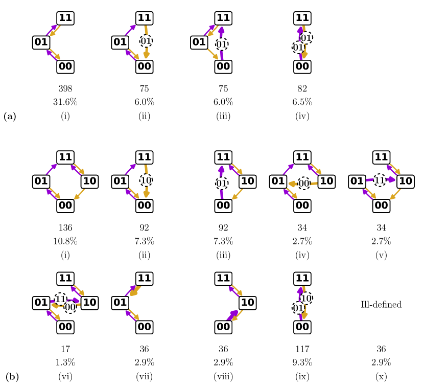
Figure 7: The thirteen $n=2$ t-graphs found by systematically constructing the candidate graphs, then checking via the design inequalities whether these are realizable; here we do not consider the GoE states. Note that, when intermediate states are ignored, graphs (a)-(ii) and (b)-(ii), and graphs (a)-(iv) and (b)-(ix) are equal, leading to the same eleven t-graphs as found previously via numerical sampling [5]. The corresponding number of total orders and associated percentages of parameter space, when eliminating simple self-loops, are shown below each graph. Note that the the sum of total order counts (1224) is higher than that obtained when GoE states are included (850). This is because transitions associated with GoE states are now allowed to be ill-defined: this includes both race conditions and self-loops occuring in a transition initiated from a GoE state (see I.2.3), as well as cases where the GoE state is persistently unstable (see section I.2). (a) T-graphs, total order counts and percentages for the $n=2$ scaffold with main loop (1, 2) (see also Fig. 6). (b) T-graphs, total order counts and percentages for the $n=2$ scaffold with main loop (2, 1). In panels (vii) and (viii), thicker arrows indicate $l=3$ avalanches; the full transition paths, not indicated in the figure, are $\{11\}\rotatebox{90.0}{$\dashleftarrow$}\{10\}\rotatebox{90.0}{$\dashleftarrow$}\{00\}\rotatebox{90.0}{$\dashrightarrow$}\{01\}$ and $\{00\}\rotatebox{90.0}{$\dashrightarrow$}\{01\}\rotatebox{90.0}{$\dashrightarrow$}\{11\}\rotatebox{90.0}{$\dashleftarrow$}\{10\}$ respectively.

In this section, we apply our framework to gain insight into the t-graph probabilities that were found using sampling [5]. We first use the design inequalities to quantify the statistical weight of a single t-graph (section IV.1). We then apply this method to all $n=2$ t-graphs found in section III, to find the percentage of graphs that is ill-defined (section IV.2).

IV.1 Domain in parameter space and counting total orders

Previously, the parameter space of switching fields has been explored through random sampling [5]. We now show how the statistical weight of a target t-graph can be quantified via the design inequalities, and corresponding partial order $P^{*}$.

To start with, for each partial order $P^{*}$ there are one or more total orders which satisfy that partial order (or ’linear extensions’, see section II.2.3) [35, 36]. The problem of generating all linear extensions for a given partial order is conceptually similar to that of generating a random linear extension, and several algorithms have been proposed based on topological sorting[37, 38, 39]. Yet, the computational time required blows up rapidly for more complex partial orders, and the general problem of generating all linear extensions - or even counting these - is in fact known to be #P-complete [40, 36]. For $n=2$, however, the number of inequalities is small, and so the problem of finding all linear extensions is manageable.

The approach we used to generate all linear extensions for $n=2$ is a breadth-first search algorithm: we add inequalities to $P^{*}$ one at a time, applying the transitive closure at each step, and let the number of added inequalities function as the algorithmic depth. The algorithm terminates when every element of the matrix is comparable (i.e., either $x>y$ or $x<y$ for all $x\neq y$), so that a total order is obtained. We find that, for example, the graph in Fig. 3a is associated with eighteen total orders of the switching fields.

As observed by Brightwell and Winkler [40], the problem of counting the number of linear extensions is closely related to that of computing the volume of a polyhedron. Namely, since there are $(n\cdot 2^{n})!$ possible permutations of the switching field order, and by symmetry each total order takes up the same volume in parameter space, the fractional volume of a t-graph is obtained by dividing its corresponding number of total orders by $(n\cdot 2^{n})!$. Applying this to the example t-graph in Fig. 3a, one obtains a fractional volume of $18/8!\approx 4.5\times 10^{-4}$.

We check this result by directly computing the volume bounded by the design inequalities. As each design inequality forms a codimension-1 hyperplane in the design space, each t-graph corresponds to an intersection of half-spaces, which is a convex polyhedron [41, 42]. This polyhedron is unbounded: we can arbitrarily increase the switching fields for a given graph as long as their order remains the same. Following the example of Keim and Paulsen [7], we generate the vertices of this polyhedron to generate a convex hull, and compute its volume using appropriate Python packages. To ensure the volume is finite, we set $U_{i}^{\pm}(S)\in[0,1]$ for all switching fields: under this convention the total volume of design space is 1, and the volume of the polyhedron corresponds directly to the probability of a t-graph under random sampling. Using this approach, we indeed find a volume of $4.5\times 10^{-4}$ for our example t-graph, in agreement with our exact result.

IV.2 The space of $n=2$-graphs

Our method for generating candidate graphs via scaffolds and trees (section III) allows to gain insight in the (relative) volume in design space occupied by different t-graphs. Here we focus in particular on the fraction of design space that leads to ill-defined t-graphs. To do so, we construct the design inequalities, the partial order $P^{*}$, and all corresponding total orders for a set of well-defined t-graphs (see sections II.2 and IV.1).

First off, since we are dealing with eight switching fields, the number of possible total orders equals $8!/2!=20160$, where we divide by $2!$ to take care of the relabeling symmetry. Each scaffold takes up an equal partition in this parameter space, as can be seen from a symmetry argument: for given state $S$, no hysteron is more likely than another to be critical. Thus, for $n=2$ each scaffold corresponds to 50 percent of parameter space, or 10080 total orders, where we note that these total orders contain both well-defined and ill-defined graphs.

If we include GoE states, the 35 well-defined t-graphs for $n=2$ interacting hysterons correspond to 850 total orders of the switching fields. Similarly, excluding GoE states, the 13 well-defined $n=2$ t-graphs correspond to 1977 total orders. This suggests that only a small part of parameter space yields well-defined t-graphs.

We have found that the vast majority of ill-defined graphs can be attributed to simple self-loops of length two — as discussed in section I.2.3, in such a case a hysteron becomes unstable in both phases as in $\{00\}\rotatebox{90.0}{$\dashrightarrow$}\{01\}\rotatebox{90.0}{$\dashleftarrow$}\{00\}\rotatebox{90.0}{$\dashrightarrow$}\{01\}\rotatebox{90.0}{$\dashleftarrow$}\dots$. We note in passing that this situation cannot occur in the additive pairwise model, but can easily occur when all switching fields are chosen independently.
We can straightforwardly prohibit such simple self-loops by enforcing additional pairwise inequalities: there are four of such inequalities for $n=2$, namely $U_{1}^{+}(00)>U_{1}^{-}(10)$, $U_{2}^{+}(00)>U_{2}^{-}(01)$, $U_{1}^{+}(01)>U_{1}^{-}(11)$ and $U_{2}^{+}(10)>U_{2}^{-}(11)$. We note that these inequalities are independent of each other and of the symmetry requirement $U_{1}^{+}(00)>U_{2}^{+}(00)$, and therefore, enforcing these inequalities reduces the number of possible total orders simply to $20160/2^{4}=1260$. Accordingly, the number of total orders per scaffold reduces to 630.

In the case where we include GoE states, the well-defined graphs still correspond to 850 total orders, as the mentioned four inequalities already emerge from each t-graph’s design inequalities. Thus, by elimination of the trivial self-loops from the set of total orders, the fraction of parameter space taken up by well-defined $n=2$ t-graphs becomes $850/1260=67.4\%$. When we exclude the GoE states, prohibiting simple self-loops via the same four inequalities yields 1224 total orders. We show the individual total order counts for each of the thirteen graphs, as well as the corresponding percentages of parameter space, in Fig. 7. The fraction of parameter space taken up by these well-defined $n=2$ t-graphs becomes $1224/1260=97.1\%$, which is qualitatively consistent with earlier estimates, although those concerned a specific parametrization of the switching fields [5].

V Conclusion, discussion and outlook

We discussed the relation between design parameters and t-graphs for the most general model for interacting hysterons. We introduced scaffolds which allow to precisely define scrambling and facilitate the systematic construction of transitions including avalanches. We presented a systematic method for obtaining the set of design inequalities for a given t-graph (or subgraph), discussed the corresponding partial order of the switching fields, and used the partial order to straightforwardly determine the realizability of t-graphs. We showed that the construction and organization of t-graphs can be seen as a three-step process: first, all scaffolds can easily be counted and generated; second, each transition in a scaffold can be selected from easily constructible finite binary trees that encode avalanches; third, the realizability of candidate graphs formed by combining scaffolds and trees can be checked using their design inequalities. As specific examples, we count all possible t-graphs for $n=2$, and when we exclude Garden-of-Eden states, we find thirteen distinct t-graphs; when we furthermore ignore differences between intermediate states, we find eleven t-graphs, consistent with an earlier estimate based on sampling the design space [5]. For $n=3$, the number of scaffolds is $96$, producing exactly 96 avalanche-free t-graphs, and when GoE states are excluded, there are 35 $n=3$ t-graphs without avalanches; including avalanches, we find more than $4.5\times 10^{12}$ candidate t-graphs, of which around $1.5\times 10^{4}$ have been found as actual t-graphs by random sampling [5]. To enter the complex design space, we show how we can count and determine the candidate graphs and realizable t-graphs for $n=2$ and $n=3$ that contain one or two $l=2$ avalanches, or one $l=3$ avalanche. We finally discuss the statistical weight of t-graphs in design space by relating it to the number of total orders consistent with a given partial order.

We stress that the rich structure of the t-graphs and design space can be seen as generalizing that of the Preisach model of non-interacting hysterons [19, 20, 4]. First, the $2n$ hysteron-dependent switching fields of the Preisach model are generalized to $n\cdot 2^{n}$ state-dependent switching fields. Second, while in the Preisach model the main loop determines all other transitions, here the scaffold can be seen as the generalization of the main loop. Third, while the ordering of the hysteron dependent switching field determines the different Preisach t-graph topologies, here we need to consider the orderings of the more numerous state-dependent switching fields. However, the occurrence of avalanches and ill-defined transitions has no obvious pendant in the Preisach model, and it is these that drive the combinatorial explosion and complexity of design space.

In closing, we list a number of important issues for future studies.

Importance of avalanches.—

Avalanches play a mixed role. On the one hand, avalanches are not required for a variety of interesting phenomena, or even can obscure their essence: scrambling, transients and multiperiodic responses under cyclic driving do not require avalanches to occur [43, 7, 10, 22, 13, 44]. Moreover, a scaffold-centered approach can simplify the design of experimental systems that exhibit transients [13, 10] or subharmonic loops [44]. On the other hand, avalanches can have a significant effect, for example allowing for transients and breaking of loop-RPM on scaffolds that are consistent with the Preisach model [13]. This suggests that an approach that focusses on the much smaller number of scaffolds, gradually adding a few avalanches of short length, may give already a good starting point to understand the statistics and typical response of systems of interacting hysterons: while adding many avalanches of longer lengths leads to a combinatorial explosion, and an even more severe growth of the corresponding number of total orders of the switching fields (these grow as $(n\cdot 2^{n})!/n!$ which already exceeds $3\times 10^{23}$ for $n=3$), the corresponding growth of the number of design inequalities suggest that such avalanche-heavy t-graphs, may only cover a small part of design space or even are not realizable. Whether such an approach truly captures the broad variety and statistics of transition graphs and memory effects remains an open question.

Specific parametrizations.—

While in this paper we consider all the switching fields to be completely independent, different parametrizations of $U_{i}^{\pm}(S)$ have been used and may be relevant in experiments [10, 26]. Most prominent are several variations of pairwise additive interactions of the form $U_{i}^{\pm}(S)=u_{i}^{\pm}{-}\Sigma_{j}c_{ij}^{\pm}s_{j}$, where $u_{i}^{\pm}$ are the bare switching fields, and the matrices $c_{ij}^{\pm}$ capture the interactions — for $c_{ij}^{\pm}\equiv 0$, we recover the Preisach model. Several further simplifications have been made: for example, one can assume that $c_{ij}^{+}=c_{ij}^{-}$; in addition one may assume reciprocity ($c_{ij}=c_{ji}$). However, both non-reciprocity and $c_{ij}^{+}\neq c_{ij}^{-}$ can be observed in experiments [10, 26, 44]. Conversely, specific experimental settings may require even more restricted interactions, such as $c_{ij}=-d_{j}$, where $d_{j}$ are positive, for serially coupled mechanical hysterons [13]. Such explicit parameterizations do not affect the structure of scaffolds, trees and candidate graphs, but significantly impact the design inequalities, either by augmentation of the design inequalities with additional constraints, or by explicit conversion of the design inequalities to the specific design parameters (such as $u_{i}^{\pm}$ and $c_{ij}^{\pm}$). Hence, specific parametrizations lead to stricter realizability conditions and a smaller group of realizable t-graphs. In some cases, specific parametrizations may even lead to qualitative restrictions on the realizable t-graphs: for example, ferromagnetic interactions ($c_{ij}^{\pm}>0$) do not allow to break (loop)-RPM, and thus cannot produce transients or subharmonic orbits [45, 46]; serial coupling ($c_{ij}=-d_{j}$) cannot produce scrambling, but can lead to breaking of (loop)-RPM via the formation of avalanches [13]. Gaining better insight on the relation between specific classes of interactions and t-graph topologies is an important topic for further study.

In the additive pairwise coupling model and its variants, requirements on the hysteron switching fields can be formulated in terms of coupling $c_{ij}^{\pm}$ between hysterons, and of the ’span’ of a single hysteron, $\sigma_{i}=u_{i}^{+}-u_{i}^{-}$. The hysteron span and coupling are identifiable in the design inequalities, even in the general model. For example, reconsidering the design inequalities in Fig. 3e, the inequality $U_{1}^{+}(00)>U_{1}^{+}(01)$ can be interpreted as a ferromagnetic coupling (positive $c_{ij}$), where hysteron 2 causes a downward (upward) shift in the up switching field of hysteron 1 upon flipping up (down). Similarly, the inequality $U_{1}^{+}(00)>U_{1}^{-}(10)$ is associated with hysteron 1 having a positive span. In fact, the conditions that we impose to prevent trivial self-loops (Section IV.2) essentially enforce that each hysteron span is always positive. Span and coupling strength may allow for a classification of different hysteron systems. First, the ratio between the coupling coefficients $c_{ij}$ and the span $\sigma_{i}$ quantifies the scale-invariant coupling strength, where the limit of zero coupling strength corresponds to the Preisach model [5, 7], and the limit of zero span corresponds to a spin model [7]; the presence of certain t-graphs and classes of t-graphs shows powerlaw scaling with coupling strength [5, 18]. A second relevant quantity is the dispersity in hysteron spans, as evidenced by the fact that even for the Preisach model, some t-graphs require hysterons to have differing spans while others do not [20, 4, 44]. An approach where the design inequalities (section II.1) and the associated partial order (section II.2) are formulated in terms of the hysteron span and coupling may provide additional insights [47].

Extended models.—

This work focussed on abstract hysterons with phenomenologically introduced interactions. More realistic models can give insight into the physical reality of hysterons, as well as the shortcomings of hysteron models, may help to establish a physical picture for their interactions, and may allow to access additional physical effects. First, for hysterons where each phase is associated with a different relation between two conjugated variables - such as force and deformation - one can explicitly work out the interactions that are mediated in networks of such hysterons [13, 26, 9]. Such enhanced models are one step in a hierarchy of increasingly realistic models, that may give insight into the mechanisms that govern hysteron interactions, as well as providing design strategies to realize metamaterials that leverage such interactions. An interesting question is if we can define enhanced hysteron models that avoid race conditions and infinite loops; conversely, it is unclear under which conditions complex energy landscapes can still be meaningfully described by interacting hysterons. Second, while (thermal) noise may lead to enhanced or suppressed memories [48], its role for interacting hysteron models is an important topic for future study. Third, many complex systems exhibit slow relaxations - determining which aspects stem from the complex transients exhibited by interacting hysterons, and which are due to slow relaxations of non-hysteron degrees of freedom remains an open question. Finally, this work, while general, focussed on the case of a few hysterons. While the continuum limit of the Preisach model has been studied in detail [49, 50], we have no continuum model for describing the statistics of large numbers of interacting hysterons.

Total order and finite state machines.—

The same t-graph topology can correspond to many total orders of the switching fields (Section IV.1). However, these total orders can lead to different responses when the system is subjected to specific driving protocols, as can be seen by considering subharmonic loops under cyclical driving [7, 5, 44], and breaking of return point memory under asymmetric driving [21]. In other words, while t-graphs describe the response to arbitrary driving, extracting qualitative information, such as whether there is a cyclical driving protocol that produces a subharmonic orbit is not easy [13]. One strategy to effectively describe the response of systems characterized by t-graphs to specific driving inputs, such as cyclic driving or sequences of driving pulses, is to use finite state machines (FSMs) [13]. In brief, the idea is that any finite t-graph has only a finite number of relevant switching fields, such that the number of, e.g., pulses in $U$ that result in a different response is also finite. Defining a finite set of symbols $\{a_{i}\}$ then allows to determine a transition table $S^{\prime}=a_{i}(S_{j})$ that maps an initial state $S_{j}$ and driving $a_{i}$ to a final state $S^{\prime}$, and therefore defines a FSM. This framework is effective in identifying specific types of responses, such as transients, for arbitrary t-graphs [13]. Moreover, this approach facilitates engineering applications, such as counting [51] and smart actuation for soft robots under a single input[52, 53, 13, 16].

The FSM framework is deeply linked with the total order of the state switching fields, with preliminary explorations indicating that any permutation in the switching fields produces a different transition table, and hence a different FSM. Hence, in addition to the design inequalities required for the t-graph topology, a more restricted partial order is required to ensure that the driving protocol leads the specific desired behavior, or to a specific FSM. Open questions for the future include how specific classes of hysteron interactions lead to, or limit, the associated FSMs and their computational power, and how to effectively design a (minimal) set of hysterons (and signals) that realize a target FSM [13, 54].

VI Acknowledgements

We gratefully acknowledge discussions with M. Mungan. M.T. and M.v.H. acknowledge funding from European Research Council Grant ERC-101019474.

References

- Keim et al. [2019] N. C. Keim, J. D. Paulsen, Z. Zeravcic, S. Sastry, and S. R. Nagel, Reviews of Modern Physics 91, 035002 (2019).
- Paulsen and Keim [2019] J. D. Paulsen and N. C. Keim, Proc. Roy. Soc. A 475 (2019).
- Mungan et al. [2019] M. Mungan, S. Sastry, K. Dahmen, and I. Regev, Phys. Rev. Lett. 123 (2019).
- Mungan and Terzi [2019] M. Mungan and M. M. Terzi, in Annales Henri Poincaré (Springer, 2019), vol. 20, pp. 2819–2872.
- van Hecke [2021] M. van Hecke, Phys. Rev. E 104 (2021).
- Lindeman and Nagel [2021] C. W. Lindeman and S. R. Nagel, Science Advances 7 (2021).
- Paulsen and Keim [2021] J. D. Paulsen and N. C. Keim, Science Advances 7 (2021).
- Das et al. [2022] S. G. Das, J. Krug, and M. Mungan, Phys. Rev. X 12 (2022).
- Shohat et al. [2021] D. Shohat, D. Hexner, and Y. Lahini (2021), eprint 2109.05212.
- Bense and van Hecke [2021] H. Bense and M. van Hecke, PNAS 118 (2021).
- Jules et al. [2022] T. Jules, A. Reid, K. E. Daniels, M. Mungan, and F. Lechenault, Phys. Rev. Research 4 (2022).
- Merrigan et al. [2022] C. Merrigan, D. Shohat, C. Sirote, Y. Lahini, C. Nisoli, and Y. Shokef, arXiv preprint arXiv:2204.04000 (2022).
- Liu et al. [2024, Accepted] J. Liu, M. Teunisse, G. Korovin, I. R. Vermaire, L. Jin, H. Bense, and M. van Hecke, PNAS (2024, Accepted).
- El Elmi and Pasini [2024] A. El Elmi and D. Pasini, Soft Matter 20, 1186 (2024).
- Muhaxheri and Santangelo [2024] G. Muhaxheri and C. D. Santangelo, arXiv preprint arXiv:2403.10721 (2024).
- Melancon et al. [2022] D. Melancon, A. E. Forte, L. M. Kamp, B. Gorissen, and K. Bertoldi, Advanced Functional Materials xx, https://doi.org/10.1002/adfm.202201891 (2022).
- Regev et al. [2021] I. Regev, I. Attia, K. Dahmen, S. Sastry, and M. Mungan, Physical Review E 103, 062614 (2021).
- Lindeman et al. [2023a] C. W. Lindeman, V. F. Hagh, C. I. Ip, and S. R. Nagel, Physical review letters 130, 197201 (2023a).
- Preisach [1935] F. Preisach, Zeitschrift für Physik 94, 277 (1935).
- Terzi and Mungan [2020] M. M. Terzi and M. Mungan, Phys. Rev. E 102 (2020).
- Lindeman et al. [2023b] C. W. Lindeman, T. R. Jalowiec, and N. C. Keim, Isolating the enhanced memory of a glassy system (2023b), eprint 2306.07177.
- Szulc et al. [2022] A. Szulc, M. Mungan, and I. Regev, The Journal of Chemical Physics 156 (2022).
- Ding and van Hecke [2022] J. Ding and M. van Hecke, The Journal of Chemical Physics 156 (2022).
- Hyatt and Harne [2023] L. P. Hyatt and R. L. Harne, Extreme Mechanics Letters 59, 101975 (2023).
- Barker et al. [1983] J. A. Barker, D. Schreiber, B. Huth, and D. H. Everett, Proceedings of the Royal Society of London. A. Mathematical and Physical Sciences 386, 251 (1983).
- Shohat and van Hecke [2024] D. Shohat and M. van Hecke, In preparation (2024).
- Ferrari et al. [2022] P. L. Ferrari, M. Mungan, and M. M. Terzi, Annales de l’Institut Henri Poincaré D (2022).
- Huffman [1954] D. A. Huffman, Journal of the Franklin Institute 257, 161 (1954).
- Grami [2022] A. Grami, Discrete Mathematics: Essentials and Applications (Academic Press, 2022).
- Warshall [1962] S. Warshall, Journal of the ACM (JACM) 9, 11 (1962).
- Dantzig et al. [1972] G. B. Dantzig, B. C. Eaves, et al. (1972).
- Dantzig and Thapa [1997] G. B. Dantzig and M. N. Thapa, The simplex method (Springer, 1997).
- Kahn [1962] A. B. Kahn, Communications of the ACM 5, 558 (1962).
- Knuth [1997] D. E. Knuth, The Art of Computer Programming: Fundamental Algorithms, volume 1 (Addison-Wesley Professional, 1997).
- Szpilrajn [1930] E. Szpilrajn, Fundamenta mathematicae 1, 386 (1930).
- Pruesse and Ruskey [1994] G. Pruesse and F. Ruskey, SIAM Journal on Computing 23, 373 (1994).
- Knuth and Szwarcfiter [1974] D. E. Knuth and J. L. Szwarcfiter, Information Processing Letters 2, 153 (1974).
- Varol and Rotem [1981] Y. L. Varol and D. Rotem, The Computer Journal 24, 83 (1981).
- Kalvin and Varol [1983] A. D. Kalvin and Y. L. Varol, Journal of Algorithms 4, 150 (1983).
- Brightwell and Winkler [1991] G. Brightwell and P. Winkler, Order 8, 225 (1991).
- [41] M. Mungan Priv. Comm.
- Grünbaum [2003] B. Grünbaum, Convex Polytopes (Springer, 2003), 2nd ed.
- Deutsch and Narayan [2003] J. M. Deutsch and O. Narayan, Physical review letters 91, 200601 (2003).
- Lishuai Jin and van Hecke [2024] H. B. Lishuai Jin, Colin Meulblok and M. van Hecke, In preparation (2024).
- Sethna et al. [1993] J. P. Sethna, K. Dahmen, S. Kartha, J. A. Krumhansl, B. W. Roberts, and J. D. Shore, Physical Review Letters 70, 3347 (1993).
- Deutsch et al. [2004] J. Deutsch, A. Dhar, and O. Narayan, Physical review letters 92, 227203 (2004).
- Teunisse and van Hecke [2024] M. Teunisse and M. van Hecke, In preparation (2024).
- Keim and Nagel [2011] N. C. Keim and S. R. Nagel, Physical review letters 107, 010603 (2011).
- Mayergoyz [1985] I. Mayergoyz, Journal of Applied Physics 57, 3803 (1985).
- Ortin [1992] J. Ortin, Journal of applied physics 71, 1454 (1992).
- Kwakernaak and van Hecke [2023] L. J. Kwakernaak and M. van Hecke, Physical Review Letters 130, 268204 (2023).
- Holmes et al. [2006] P. Holmes, R. J. Full, D. Koditschek, and J. Guckenheimer, SIAM review 48, 207 (2006).
- Overvelde et al. [2015] J. T. Overvelde, T. Kloek, J. J. D’haen, and K. Bertoldi, Proceedings of the National Academy of Sciences 112, 10863 (2015).
- Byun et al. [2024] J. Byun, A. Pal, J. Ko, and M. Sitti, Nature Communications 15, 2933 (2024).