FIELD METHOD APPROACH IN THE FACTORIZATION OF NONLINEAR SECOND ORDER DIFFERENTIAL EQUATIONS
Abstract
Abstract. In this paper, the general solution of second-order nonlinear differential equations of Liénard type is obtained within the nonlinear factorization method of Rosu and Cornejo-Pérez by the so-called field method approach. This method is based on writing the factorization conditions in the dynamical systems form and requires to assume that the intermediate function that occurs in the factorization be dependent not only on the dependent variable of the nonlinear equation, but also on the independent variable. The method is applied to several cases of Liénard type equations which are written in a commutative factorization form and their general solutions are obtained by solving Bernoulli differential equations.
Keywords: Liénard equation; commutative factorization; factorization condition; Sharma-Tasso-Olver equation; field method.
I Introduction
Nonlinear differential equations of the Liénard type lrbook ; hl16
| (1) |
where the dot denotes the derivative and and are arbitrary real functions, serve as an important class of ordinary differential equations (ODE’s) with widespread applications to a huge number of physical, chemical, biological, and engineering systems, see getal and references therein. Even linear differential equations corresponding to and const. can be included in the Liénard class.
The goal of this paper is to present a new approach to the nonlinear factorization method introduced by two of the authors a couple of decades ago rcp1 ; rcp2 which leads to exact solutions of many nonlinear equations in a simple way. The proposed method is similar to the so-called field method introduced by Vujanovic vuj1 ; vuj2 , see also kov1 ; kov2 , which states that for any nonconservative, holonomic, rheonomic, dynamical system whose evolution is given in the dynamical form
| (2) |
we can choose one coordinate of the system, say , which can be selected as a field depending on time and the rest of the coordinates
| (3) |
Taking the total time derivative with respect to time of Eq. (3) and using the last equations of (2), one can write the dynamical system as a quasi-linear first order partial differential equation given by
| (4) |
The complete solution of Eq. (4) is of the form
| (5) |
where is an arbitrary constant. In the nonlinear factorization method, the solution (5) can be used to construct the general solution of (1).
In this paper, we implement this field approach into the factorization method and show that one can obtain the general solution of the problem for the commutative factorization setting of nonlinear ODE’s in an easy and straightforward way.
Section II of the paper describes the implementation of the field method approach in the framework of commutative factorizations. In section III, we present some specific examples of the field method approach as applied to factored nonlinear ODE’s, including a unifying treatment of the examples. Finally, the conclusions are summarized in the last section.
II Factorization and Field Method Approach
Equation (1) can be factorized in the form
| (6) |
under the conditions rcp1 ; rcp2
| (7) | |||
| (8) |
From (8), one can see that if is a homogeneous polynomial then one can choose the factorization functions as complementary pairs in the set of divisors of the nonhomogeneous polynomial , a hint that reveals the efficiency of this factorization method in the case of polynomial nonlinearities. The commutative factorization setting can be achieved by demanding the following conditions
| (9) | ||||
| (10) | ||||
| (11) |
which implies that the two factorization functions differ only by a constant, i.e. .
Rosu and Cornejo-Pérez considered initially only , but also the extension to has been discussed in the literature wl2008 ; rmex17 . Borrowing from the field method, we assume now , which yields the following coupled ODE’s for the factorized Eq. (6),
| (12) | |||
| (13) |
which can be also written in the matrix dynamical systems form
| (14) |
According to the chain rule, the system of equations (12)-(13) can be rewritten as the quasi-linear first order partial differential equation
| (15) |
which can be solved by proposing the ansatz vuj1 ; kovacic2003 . Then, for the function , one obtains the first-order differential equation
| (16) |
If the commutative factorization condition is considered, then the subtraction of factorization functions holds for const., and (16) reduces to
| (17) |
which is a Bernoulli differential equation of nonlinear order two. Its solution is given as follows
| (18) | |||||
| (19) | |||||
| (20) |
where is an integration constant. This last result allows to rewrite the first-order ODE (12) in the form
| (21) |
which is a Bernoulli differential equation with the nonlinearity of one order higher than the order of the ’s. Its solution provides the general solution of Eq. (1) factored in the (commutative) form given in Eq. (6).
It is worth mentioning that for the complex case , the following symmetric factorization of Eq. (1) is necessary
| (22) |
from where the following compatible first order ODE is obtained
| (23) |
or by using Eq. (20), we obtain for this case the following Bernoulli differential equation
| (24) |
From the expressions of , one can see that only the one containing the tangent function is trigonometric. Therefore, taking into account that the general solutions of the Bernoulli equations can be written as logarithmic derivatives, then one may obtain periodic (isochronous) solutions of Eq. (21) only in the case of the trigonometric .
III Some applications
To show how the field method works in practice, we discuss three simple Liénard equations of the cubic oscillator type, one quintic oscillator case, the first corresponding to the inverse power , and the others corresponding to the trigonometric . The general higher-order nonlinear Liénard equations for which the field method can be applied is also presented.
1. A pure cubic anharmonic oscillator with nonlinear damping
Let us consider the following cubic anharmonic oscillator equation
| (25) |
which admits the commutative factorization
| (26) |
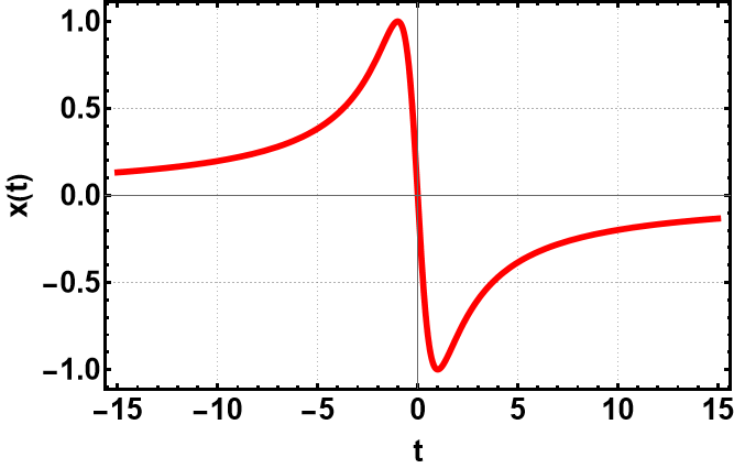
where , and . Then, by substituting the corresponding function from Eq. (18) into Eq. (21), we obtain the Bernoulli equation
| (27) |
whose general solution is given as follows
| (28) |
where is an integration constant, while appears as a parameter in the Bernoulli differential equation, which, from Eq. (28), can be also interpreted as a constant fixed through the initial conditions applied to Eq. (25). In Fig. 1, a particular case of the solution given in Eq. (28) is displayed.
2. Same cubic anharmonic oscillator with added harmonic term
Let us consider now the more general nonlinear ODE
| (29) |
which admits the commutative factorization
| (30) |
where , , and is an imaginary constant. Thus for this case, (24) takes the form
| (31) |
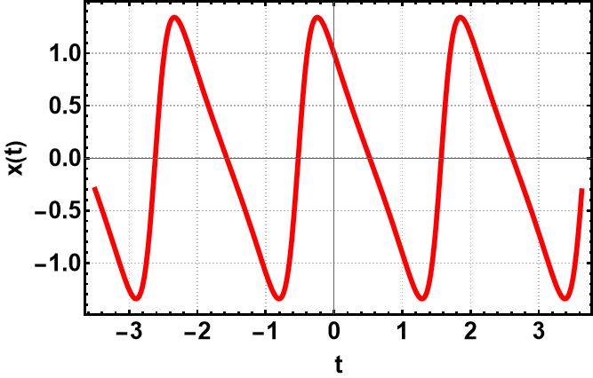
with solution given as follows
| (32) |
where is an integration constant, while has a role similar to of the previous case. If , the general solution (32) is an isochronous solution of frequency . In Fig. 2, we present the plot corresponding to the solution given in Eq. (32) for , , , and .
3. Travelling wave solution of the Sharma-Tasso-Olver equation
The Sharma–Tasso–Olver (STO) equation is an odd order nonlinear partial differential equation of the Burgers hierarchy that plays a very important role in sciences and engineering fields, for instance plasma, nonlinear optics, quantum fields with many solution methods available in the literature ll05 ; ww07 . The STO equation is given by
| (33) |
If we consider Eq. (33) in the moving reference frame under the transformation such that and integrating once we have the ODE
| (34) |
where is an integration constant. Next, we make the following shift transformation , where is a constant that satisfies the following cubic equation
| (35) |
The roots of this equation are classified according to the discriminant
If , there is only one real root, and if , all the three roots are real.
Through the shift transformation, one obtains the following second order nonlinear ODE
| (36) |
The latter equation can be factored in the following form
| (37) |
only for the case of the real roots of the cubic equation (35). For the special case when we choose the integration constant , where , and , we have the real roots for the cubic equation given by . Therefore, from the factorization given in Eq. (37), we have that , which implies . Consequently, the general solution of Eq. (37) is obtained by solving the following Bernoulli differential equation
| (38) |
with solution given as follows
| (39) |
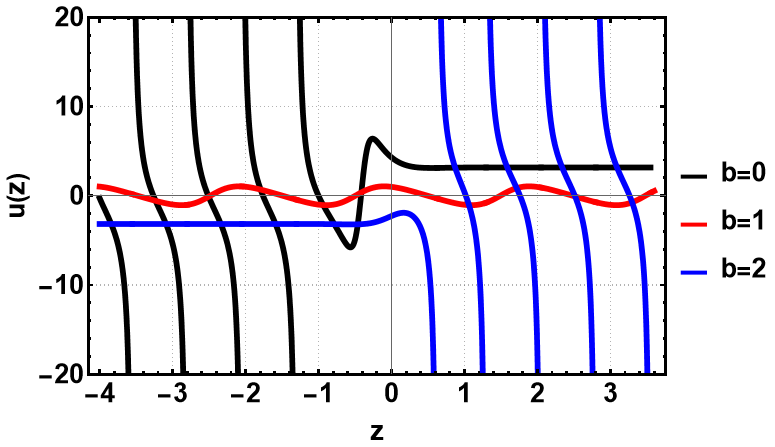
where and are integration constants. Because of the exponential function in the denominator, the solutions with periodic singularities in at least one direction can be avoided only in the case for which an isochronous solution similar to the isochronous solution (32) is obtained if . In Fig. 3, the plots corresponding to the particular STO solution obtained from Eq. (39) for , , , , and the three values of the shift parameter are displayed, showing the various types of solutions that can be obtained in this case.
4. Wilson polynomial Liénard equation
The Wilson polynomial Liénard equation WilsonL is the following particular case of quintic-cubic Duffing-van der Pol equation
| (40) |
It was the first example of Liénard equation with an algebraic hyperelliptic limit cycle for and also admits the commutative factorization
| (41) |
For this case the constant is
| (42) |
and the Bernoulli equation (21) has the trigonometric form
| (43) |
whose general solution is
| (44) |
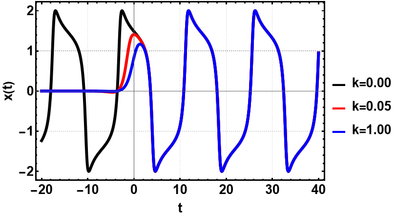
where and are integration constants. In Fig. 4, for and , one can observe the isochronous solution (44) when , and the way in which the isochronicity is lost for and .
5. A unifying treatment of the previous examples
Liénard equations of the type
| (45) |
can be factored with
| (46) |
which satisfy the commutative factorization condition of the form
| (47) |
implying the three possible cases of as in (18)-(20), but with replaced by .
The corresponding Bernoulli differential equation for reads
| (48) |
with the solution
| (49) |
where and is an arbitrary integration constant. This solution can be also written in the logarithmic derivative form
| (50) |
and represents the general Liénard solution of (45) since it depends on two arbitrary constants. The choice of a positive sign in front of the parenthesis for the factoring functions and in (46), yields a similar factorization scheme whose equivalence is obtained through and , however the same form of general solution given in Eq. (49) is obtained.
The factoring functions in (46) cover all the afore discussed particular cases and some others as well. Indeed, for , and , we have the linear damped oscillator case, for and , the nonlinear oscillator of the second case is obtained, and corresponds to the third case, and provides the STO case, and corresponds to equation (4) in iacono which has as a particular case the equation (29), a case with all nonzero and corresponds to a cubic-quintic Duffing-van der Pol unforced equation siewe , and the list can be continued.
IV Conclusion
An alternative way of solving the nonlinear commutative factorization setting previously studied in getal has been provided here. An intermediate function in the method is assumed to depend explicitly on the independent variable of the factored equation, aside to the dependent variable. This leads to a quasi-linear differential equation which can be solved and allows one to obtain the general solution of the problem for many commutative factorization settings. When a separable form in the two variables of the intermediate function is assumed, the dependent variable of the nonlinear equation is found to satisfy a Bernoulli differential equation with parameters and nonlinear part that depend on the factorization functions which is easily solved and leads to the general solution of the nonlinear second-order differential equation. This alternative method has been applied to several illustrative cases of Liénard equations and can be used for many equations by employing polynomial factoring functions that differ by a constant.
CRediT authorship contribution statement
G. González: Conceptualization, Writing – original draft.
O. Cornejo-Pérez: Methodology, Validation.
H.C. Rosu: Formal analysis, Writing - review and editing.
Declaration of competing interests
The authors declare that they have no known competing financial interests or personal relationships
that could have appeared to influence the work reported in this paper.
Data availability statement
No data have been used in this paper.
Acknowledgments
G.G. would like to acknowledge support by the program Cátedras Conahcyt through project 1757 and from project A1-S-43579 of SEP-CONAHCYT Ciencia Básica and Laboratorio Nacional de Ciencia y Tecnología de Terahertz.
References
- (1) Lakshmanan M, Rajasekar S. Nonlinear Dynamics: Integrability, Chaos, and Patterns. 2003; Springer: Heidelberg. https://doi.org/10.1007/978-3-642-55688-3
- (2) Harko T, Lian S-D. Exact solutions of the Liénard and generalized Liénard type ordinary differential equations obtained by deforming the phase space coordinates of the linear harmonic oscillator. J. Eng. Math. 2016; 98: 93-111. https://doi.org/10.1007/s10665-015-9812-z
- (3) González G, Rosu HC, Cornejo-Pérez O, Mancas SC. Factorization conditions for nonlinear second-order differential equations. 2024; In the NMMP-2022 proceedings book: Springer. arXiv:2211.01541, https://doi.org/10.48550/arXiv.2211.01541
- (4) Rosu HC, Cornejo-Pérez O. Supersymmetric pairing of kinks for polynomial nonlinearities. Phys. Rev. E 2005; 71: 046607. https://doi.org/10.1103/PhysRevE.71.046607
- (5) Cornejo-Pérez O, Rosu HC. Nonlinear second order ODE’s: Factorizations and particular solution. Prog. Theor. Phys. 2005; 114: 533-538. https://doi.org/10.1143/PTP.114.533
- (6) Vujanovic B. On the integration of the nonconservative Hamilton’s dynamical equations. Int. J. Eng. Sci. 1981; 19: 1739-1747. https://doi.org/10.1016/0020-7225(81)90164-6
- (7) Vujanovic BD, Jones SE. Variational Methods in Nonconservative Phenomena. 1989; Academic: Boston. ISBN: 9780080926421
- (8) Kovacic I. Analysis of a weakly non-linear autonomous oscillator by means of the field method. Int. J. Non-Linear Mech. 2005; 40: 775-784. https://doi.org/10.1016/j.ijnonlinmec.2004.06.009
- (9) Kovacic I. Invariants and approximate solutions for certain non-linear oscillators by means of the field method. Appl. Math. Comp. 2010; 215: 3482-3487. https://doi.org/10.1016/j.amc.2009.10.025
- (10) Wang DS, Li H. Single and multi-solitary wave solutions to a class of nonlinear evolution equations. J. Math. Anal. Appl. 2008; 343: 273-298. https://doi.org/10.1016/j.jmaa.2008.01.039
- (11) Rosu HC, Cornejo-Pérez O, Pérez-Maldonado M, Belinchón JA. Extension of a factorization method of nonlinear second order ODE’s with variable coefficients. Rev. Mex. Fís. 2017; 63: 218-222. ISSN:0035-001X
- (12) Kovacić I. Bohlin’s like integrals for nonconservative mechanical systems. J. Electrical Eng. 2002; 53(12s): 60-63. http://www.journals4free.com/link.jsp?l=14507657
- (13) Lian Z-j, Lou SY, Symmetries and exact solutions of the Sharma–Tass–Olver equation. Nonlinear Anal. 2005; 63: e1167-e1177. https://doi.org/10.1016/j.na.2005.03.036
- (14) Wazwaz A-M. New solitons and kinks solutions to the Sharma-Tasso-Olver equation. Appl. Math. Comp. 1997; 188: 1205-1213. https://doi.org/10.1016/j.amc.2006.10.075
- (15) Wilson JC. Algebraic periodic solutions of . Contrib. Differ. Equ. 1964; 3: 1-20.
- (16) Iacono R, Russo F. Class of solvable nonlinear oscillators with isochronous orbits. Phys. Rev. E 2011; 83: 027601. https://doi.org/10.1103/PhysRevE.83.027601
- (17) Siewe Siewe M, Moukam Kakmeni FM, Tchawona C, Resonant oscillation and homoclinic bifurcation in a -van der Pol oscillator. Chaos, Solitons, and Fractals 2004; 21: 841-853. https://doi.org/10.1016/j.chaos.2003.12.014