How Does Message Passing Improve Collaborative Filtering?

Abstract.

Collaborative filtering (CF) has exhibited prominent results for recommender systems and been broadly utilized for real-world applications. A branch of research enhances CF methods by message passing used in graph neural networks, due to its strong capabilities of extracting knowledge from graph-structured data, like user-item bipartite graphs that naturally exist in CF. They assume that message passing helps CF methods in a manner akin to its benefits for graph-based learning tasks in general (e.g., node classification). However, even though message passing empirically improves CF, whether or not this assumption is correct still needs verification. To address this gap, we formally investigate why message passing helps CF from multiple perspectives and show that many assumptions made by previous works are not entirely accurate. With our curated ablation studies and theoretical analyses, we discover that (i) message passing improves the CF performance primarily by additional representations passed from neighbors during the forward pass instead of additional gradient updates to neighbor representations during the model back-propagation and (ii) message passing usually helps low-degree nodes more than high-degree nodes. Utilizing these novel findings, we present Test-time Aggregation for Collaborative Filtering , namely TAG-CF, a test-time augmentation framework that only conducts message passing once at inference time. The key novelty of TAG-CF is that it effectively utilizes graph knowledge while circumventing most of notorious computational overheads of message passing. Besides, TAG-CF is extremely versatile can be used as a plug-and-play module to enhance representations trained by different CF supervision signals. Evaluated on six datasets (i.e., five academic benchmarks and one real-world industrial dataset), TAG-CF consistently improves the recommendation performance of CF methods without graph by up to 39.2% on cold users and 31.7% on all users, with little to no extra computational overheads. Furthermore, compared with trending graph-enhanced CF methods, TAG-CF delivers comparable or even better performance with less than 1% of their total training time. Beside the promising cost-effectiveness, we show that test-time aggregation in TAG-CF improves recommendation performance in similar ways as the training-time aggregation does, demonstrating the legitimacy of our findings w.r.t. how does message passing improves CF.

1. Introduction

Recommender systems are essential in improving users’ experiences on web services, such as product recommendations (wang2021dcn, ; schafer1999recommender, ), video recommendations (gomez2015netflix, ; van2013deep, ), friend suggestions (sankar2021graph, ; ying2018graph, ), etc. In particular, recommender systems based on collaborative filtering (CF) have shown superior performance (rendle2009bpr, ; koren2021advances, ; chen2023bias, ). CF methods use preferences for items by users to predict additional topics or products a user might like (su2009survey, ). These methods typically learn a unique representation for each user/item and an item is recommended to a user according to the similarity of their representations (he2017neural, ; wang2015collaborative, ).

One popular line of research explores Graph Neural Networks (GNNs) for CF, exhibiting improved results compared with CF frameworks without the utilization of graphs (wu2022graph, ; he2020lightgcn, ; wang2019neural, ; yu2022graph, ; cai2023lightgcl, ; wang2020disentangled, ). The key mechanism behind GNNs is message passing, where each node aggregates information from its neighbors in the graph, and information from neighbors that are multiple hops away can be acquired by stacked message passing layers (kipf2016semi, ; velivckovic2017graph, ; hamilton2017inductive, ). During the model training, traditional CF methods directly fetch user/item representations of an observed interaction (e.g., purchase, friending, click, etc.) and enforce their pair-wise similarity (rendle2009bpr, ). Graph-enhanced CF methods extend this scheme by conducting stacked message passing layers over the user-item bipartite graph, and harnessing the resulting user and item representations to calculate a pair-wise affinity.

A recent study (he2020lightgcn, ) shows that removing several significant components of the message passing layer (e.g., learnable transformation parameters) greatly enhances GNNs’ performance for CF. Its proposed method (LightGCN) achieves promising performance by linearly aggregating neighbor representations without any transformation, and it has been used as the de facto backbone model for later graph-based methods due to its simple and effective design (cai2023lightgcl, ; yu2022graph, ; wu2021self, ). However, this observation contradicts GNN architectures for classic graph learning tasks, where GNNs without these components severely under-perform (oloulade2021graph, ; wang2021bag, ). Additionally, existing research (he2020lightgcn, ; wang2019neural, ) assumes that the contribution of message passing for CF is similar to that for graph learning tasks in general (e.g., node classification or link prediction) - they posit that node representations are progressively refined by their neighbor information and the performance gain is positively proportional to the neighborhood density as measured in node degrees (tang2020investigating, ). However, according to our empirical studies in Section 3.2, message passing in CF improves low-degree users more than high-degree users, which also contradicts GNNs’ behaviors for classic tasks (tang2020investigating, ; hu2022tuneup, ). In light of these inconsistencies between the behaviors of message passing for CF and classic graph learning tasks, we ask:

What role does message passing really
play for collaborative filtering?

In this work, we investigate contributions brought by message passing for CF from two perspectives. Firstly, we unroll the formulation of message passing layer and show that its performance improvement could either come from additional representations passed from neighbors during the forward pass or accompanying gradient updates to neighbor representations during the model back-propagation. With rigorously designed ablation studies, we empirically demonstrate that gains brought by the forward pass dominate those by the back-propagation. Furthermore, we analyze the performance distribution w.r.t. the user degree (i.e., the number of interactions per user) with or without message passing and discover that the message passing in CF improves low-degree users more compared to high-degree users. For the first time, we connect this phenomenon to Laplacian matrix learning (zhu2021interpreting, ; dong2019learning, ; dong2016learning, ), and theoretically show that popular supervision signals (rendle2009bpr, ; wang2022towards, ) for CF inadvertently conduct message passing in the back-propagation even without treating the input data as a graph. Hence, when message passing is applied, high-degree users demonstrate limited improvement, as the benefit of message passing for high degree nodes has already been captured by the supervision signal.

With the above takeaways, we present Test-time Aggregation for Collaborative Filtering , namely TAG-CF. Specifically, unlike other graph CF methods, TAG-CF does not require any message passing during training. Instead, it is a test-time augmentation framework that only conducts a single message-passing step at inference time, and effectively enhances representations inferred from different CF supervision signals. The test-time aggregation is inspired by our first perspective that, within total performance gains brought by message passing, gains from the forward pass dominate those brought by the additional back-propagation. Applying message passing only at test time avoids repetitive queries (i.e., once per node and epoch) for representations of surrounding neighbors, which grow exponentially as the number of layers increases. Moreover, following our second perspective that message passing helps low-degree nodes more in CF, we further offload the cost of TAG-CF by applying the one-time message passing only to low-degree nodes. In short, we summarize our contributions as:

• This is the first work that formally investigates why message passing helps collaborative filtering. We demonstrate that message passing in CF improves the performance primarily by additional representations passed from neighbors during the forward pass instead of accompanying gradient updates to neighbors during the back-propagation, and prove that message passing helps low-degree nodes more than high-degree nodes.

• Given our findings, we propose TAG-CF, an efficient yet effective test-time aggregation framework to enhance representations inferred by different CF supervision signals such as BPR and DirectAU. Evaluated on six datasets, TAG-CF consistently improves the performance of CF methods without graph by up to 39.2% on cold users and 31.7% on all users, with little to no extra computational overheads. Furthermore, compared with trending graph-enhanced CF methods, TAG-CF delivers comparable or even better performance with less than 1% of their total training time.

• Beside promising cost-effectiveness, we show that test-time aggregation in TAG-CF improves the recommendation performance in similar ways as the training-time aggregation does, further demonstrating the legitimacy of our findings.

2. Preliminaries and Related Work

Collaborative Filtering. Given a set of users, a set of items, and interactions between users and items, collaborative filtering (CF) methods aim at learning a unique representation for each user and item, such that user and item representations can reconstruct all observable interactions (rendle2009bpr, ; wang2022towards, ; koren2009matrix, ). CF methods based on matrix factorization directly utilize the inner product between a pair of user and item representations to infer the existence of their interaction (koren2009matrix, ; rendle2009bpr, ). Further leveraging nonlinearities, CF methods based on neural predictors use multi-layer feed-forward neural networks that take user and item representations as inputs and output prediction results (he2017neural, ; zhang2019deep, ). Let $\mathcal{U}$ and $\mathcal{I}$ denote the user set and item set respectively, with user $u_{i}\in\mathcal{U}$ associated with an embedding $\mathbf{u}_{i}\in\mathbb{R}^{d}$ and item $i_{i}\in\mathcal{U}$ associated with $\mathbf{i}_{i}\in\mathbb{R}^{d}$, the similarity $s_{ij}$ between user $u_{i}$ and item $i_{j}$ is formulated as $s_{ij}=\hat{\mathbf{u}}_{i}^{\intercal}\cdot\hat{\mathbf{i}}_{j}$.

Graph Neural Networks. Graph neural networks (GNNs) are powerful learning frameworks to extract representative information from graphs (kipf2016semi, ; velivckovic2017graph, ; hamilton2017inductive, ; xu2018representation, ; ju2023let, ; fan2022heterogeneous, ; ju2023let, ). They aim to map each input node into low-dimensional vectors, which can be utilized to conduct either graph-level (xu2018powerful, ) or node-level tasks (kipf2016semi, ). Most GNNs explore layer-wise message passing (gilmer2017neural, ), where each node iteratively extracts information from its first-order neighbors, and information from multi-hop neighbors can be captured by stacked layers. Given a graph $\mathcal{G}=(\mathcal{V},\mathcal{E})$ and node features $\mathbf{X}\in\mathbb{R}^{|\mathcal{V}|\times d}$, graph convolution in GCN (kipf2016semi, ) at $k$-th layer is formulated as:

(1) $$\mathbf{h}_{i}^{(k+1)}=\sigma(\sum_{j\in\mathcal{N}(i)\cup{i}}\frac{1}{\sqrt{|N(i)|}\sqrt{|N(j)|}}\mathbf{h}_{j}^{(k)}\cdot\mathbf{W}^{(k)}),$$

where $\mathbf{h}_{i}^{0}=\mathbf{x}_{i}$, $\mathcal{N}(i)$ refers to the set of direct neighbors of node $i$, and $\mathbf{W}^{(k)}\in\mathbb{R}^{d^{k}\times d^{(k+1)}}$ refers to parameters at the $k$-th layer transforming the node representation from $d^{k}$ to $d^{(k+1)}$ dimension.

Recent works (ma2021homophily, ; ma2021unified, ) have shown that GNNs make predictions based on the distribution of node neighborhoods. Moreover, GNNs’ performance improvement for high-degree nodes is typically better than for low-degree nodes (tang2020investigating, ; hu2022tuneup, ; ju2024graphpatcher, ; guo2024node, ). They posit that node representations are progressively refined by their neighbor information and the performance gain is positively proportional to the neighborhood density as measured in node degrees.

Message Passing for Collaborative Filtering. Recent research tends to apply the message passing scheme in GNNs to CF (he2020lightgcn, ; wang2019neural, ; pal2020pinnersage, ; gao2022graph, ; shi2020heterogeneous, ; xia2021graph, ). In CF, they mostly conduct message passing between user-item bipartite graphs and utilize the resultant representations to calculate user-item similarities. For instance, NGCF (wang2019neural, ) directly migrates the message passing scheme in GNNs (similar to Equation 1) and applies it to bipartite graphs in CF. LightGCN (he2020lightgcn, ) simplifies NGCF (wang2019neural, ) by removing certain components (i.e., the self-loop, learning parameters for graph convolution, and activation functions) and further improves the recommendation performance compared with NGCF. The simplified parameter-less message passing in LightGCN can be expressed as:

(2) $$\mathbf{u}_{i}^{(k)}=\sum_{i_{j}\in N(u_{i})}\frac{1}{\sqrt{|N(u_{i})|}\sqrt{|N(i_{j})|}}\mathbf{i}_{j}^{(k-1)},$$

(3) $$\mathbf{i}_{i}^{(k)}=\sum_{u_{j}\in N(i_{i})}\frac{1}{\sqrt{|N(i_{i})|}\sqrt{|N(u_{j})|}}\mathbf{u}_{j}^{(k-1)},$$

where $N(\cdot)$ refers to the set of items or users that the input interacts with, $\mathbf{u}_{i}^{(0)}=\mathbf{u}_{i}$, and $\mathbf{i}_{i}^{(0)}=\mathbf{i}_{i}$. With $K$ layers, the final user/item representations and their similarities are constructed as:

(4) $$\hat{\mathbf{u}}_{i}=\frac{1}{K+1}\sum_{k=0}^{K}\mathbf{u}_{i}^{(k)},\;\;\hat{\mathbf{i}}_{i}=\frac{1}{K+1}\sum_{k=0}^{K}\mathbf{i}_{i}^{(k)},\;\;s_{ij}=\hat{\mathbf{u}}_{i}^{\intercal}\cdot\hat{\mathbf{i}}_{j}.$$

According to results reported in LightGCN and NGCF (he2020lightgcn, ; wang2019neural, ; chang2021sequential, ; gao2023survey, ) and empirical studies we provide in this work (i.e., Table 2 and Table 5), incorporating message passing to CF methods without graphs (i.e., matrix factorization methods (rendle2009bpr, ; he2017neural, )) can improve the recommendation performance by up to 20%. Utilizing LightGCN as the backbone model, later works try to further improve the performance by incorporating self-supervised learning signals (lin2022improving, ; yu2022graph, ; cai2023lightgcl, ; yu2021self, ; wei2021contrastive, ; ju2022multi, ). Graph-based CF methods assume that the contribution of message passing for CF is similar to that for graph learning tasks in general (e.g., node classification or link prediction). However, whether or not this assumption is correct still needs verification, even though message passing empirically improves CF. There also exists a branch of research that aims at accelerating or simplifying message passing in CF by adding graph-based regularization terms during the training (shen2021powerful, ; mao2021ultragcn, ; peng2022svd, ; xia2023graph, ). While promising, they still repetitively query representations of adjacent nodes during the training.

3. How Does Message Passing Improve Collaborative Filtering?

In this section, we demonstrate the reason behind why message passing helps collaborative filtering from two major perspectives: Firstly, we focus on inductive biases brought by the message passing explored in LightGCN, the de facto backbone model for graph-based CF methods. Secondly, we consider the performance improvement on different node subgroups w.r.t. the node degree with and without message passing.

3.1. Neighbor Information vs. Accompanying Gradients from Message Passing

Following the definition in Equation 3, given a one-layer LightGCN, we unroll the calculation of the similarity $s_{ij}$ between any user $u_{i}$ and item $i_{j}$ as the following:

$$s_{ij}=\Big{(}\mathbf{u}_{i}+\sum_{i_{n}\in N(u_{i})}\frac{1}{\sqrt{|N(u_{i})|}\sqrt{|N(i_{n})|}}\mathbf{i}_{n}\Big{)}^{\intercal}$$

$$\;\;\;\;\;\cdot\Big{(}\mathbf{i}_{j}+\sum_{u_{n}\in N(i_{j})}\frac{1}{\sqrt{|N(i_{j})|}\sqrt{|N(u_{n})|}}\mathbf{u}_{n}\Big{)}$$

$$\;\;\;=\;\mathbf{u}_{i}^{\intercal}\cdot\mathbf{i}_{j}+\sum_{u_{n}\in N(i_{j})}\frac{1}{\sqrt{|N(i_{j})|}\sqrt{|N(u_{n})|}}\mathbf{u}_{i}^{\intercal}\cdot\mathbf{u}_{n}$$

(5) $$\;\;\;\;\;\;\;\;\;\;\;\;\;\;\;\;\;\;+\sum_{i_{n}\in N(u_{i})}\frac{1}{\sqrt{|N(u_{i})|}\sqrt{|N(i_{n})|}}\mathbf{i}_{n}^{\intercal}\cdot\mathbf{i}_{j}$$

$$+\sum_{i_{n}\in N(u_{i})}\sum_{u_{n}\in N(i_{j})}\frac{1}{\sqrt{|N(u_{i})|}\sqrt{|N(i_{n})|}\sqrt{|N(i_{j})|}\sqrt{|N(u_{n})|}}\mathbf{i}_{n}^{\intercal}\cdot\mathbf{u}_{n}.$$

With derived similarities between user-item pairs, their corresponding representations can be updated by objectives (e.g., BPR (rendle2009bpr, ) and DirectAU (wang2022towards, )) that enforce the pair-wise similarity between representations of user-item pairs in the training data.

Table 1. Performance of LightGCN variants.

Method	Yelp-2018	Gowalla	Amazon-book
NDCG@20
LightGCN	6.36	9.88	8.13
w/o grad.	6.16  (3.1%$\downarrow$)	9.87  (0.1%$\downarrow$)	7.80  (4.1%$\downarrow$)
w/o neigh. info	4.71 (25.9%$\downarrow$)	6.95 (29.7%$\downarrow$)	6.95 (14.5%$\downarrow$)
w/o both	6.09  (4.2%$\downarrow$)	9.83  (0.5%$\downarrow$)	7.75  (4.7%$\downarrow$)
Recall@20
LightGCN	11.21	18.53	12.97
w/o grad.	10.87  (3.0%$\downarrow$)	18.51  (0.1%$\downarrow$)	12.81  (1.2%$\downarrow$)
w/o neigh. info	8.44 (24.7%$\downarrow$)	13.06 (29.5%$\downarrow$)	11.25 (13.3%$\downarrow$)
w/o both	10.71  (4.5%$\downarrow$)	18.42  (0.6%$\downarrow$)	12.57  (3.1%$\downarrow$)

CF methods without the utilization of graphs directly calculate the similarity between a user and an item with their own representations (i.e., $s_{ij}=\mathbf{u}_{i}^{\intercal}\cdot\mathbf{i}_{j}$), which aligns with the first term in Equation 5. Compared to the formulation in Equation 5, we can see that three additional similarity terms are introduced as inductive biases: similarities between users who purchase the same item (i.e., $\mathbf{u}_{i}^{\intercal}\cdot\mathbf{u}_{n}$), between items that share the same buyer (i.e., $\mathbf{i}_{n}^{\intercal}\cdot\mathbf{i}_{j}$), and between neighbors of an observed interaction (i.e., $\mathbf{i}_{n}^{\intercal}\cdot\mathbf{u}_{n}$). With these three additional terms from message passing, we reason that the performance improvement brought by message passing to CF methods without graph could come from (i) additional neighbor representations during the forward pass (i.e., numerical values of three extra terms in Equation 5), or (ii) accompanying gradient updates to neighbors during the back-propagation.

To investigate the origin of the performance improvement brought by message passing, we designed two variants of LightGCN. The first one (LightGCN${}_{\text{w/o neigh. info}}$) shares the same forward and backward procedures as LightGCN during the training but does not conduct message passing during the test time. In this variant, additional gradients brought by message passing are maintained as part of the resulting model, but information from neighbors are ablated. In the second variant (LightGCN${}_{\text{w/o grad.}}$), the model shares the same forward pass but drops gradients from these three additional terms during the backward propagation. Besides these two variants, we also experiment on LightGCN without message passing, denoted as LightGCN${}_{\text{w/o both}}$, a matrix factorization model with the same supervision signal (i.e., BPR loss). Implementation details w.r.t. this experiment are in Appendix C.

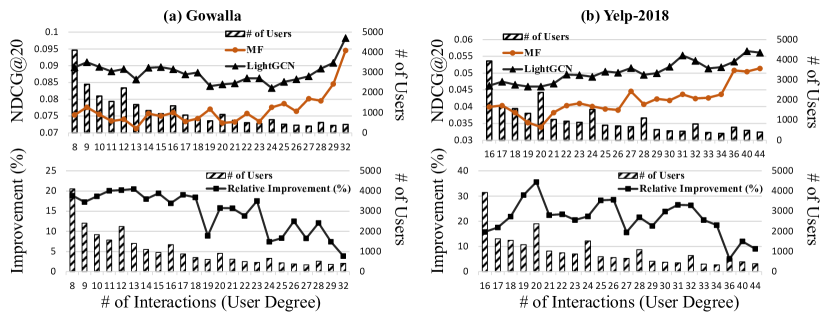
Figure 1. Performances of LightGCN and Matrix Factorization w.r.t. the user degree across datasets. The performance improvement brought by message passing decreases as the user degree goes up.

From Table 1, we observe that the performance of all variants is downgraded compared with LightGCN, with the most significant degradation on LightGCN${}_{\text{w/o neigh. info}}$. This phenomenon indicates that (i) both additional representations passed from neighbors during the forward pass and accompanying gradient updates to neighbors during the back-propagation help the recommendation performance, and (ii) within total performance gains brought by message passing, gains from the forward pass dominate those brought by the back-propagation. Comparing LightGCN with LightGCN${}_{\text{w/o grad.}}$, we notice that the incorporation of gradient updates brought by message passing is relatively incremental (i.e., $\sim$2%). However, to facilitate these additional gradient updates for slightly better performance, LightGCN is required to conduct message passing at each batch, which brings tremendous additional overheads.

3.2. Message Passing in CF Helps Low-degree Users More Compared with High-degrees

Both empirical and theoretical evidence have demonstrated that GNNs usually perform satisfactorily on high-degree nodes with rich neighbor information but not as well on low-degree nodes (tang2020investigating, ; hu2022tuneup, ). While designing graph-based model architectures for CF, most existing methods directly borrow this line of observations (wang2019neural, ; he2020lightgcn, ) and assume that the contribution of message passing for CF is similar to that for graph learning tasks in general. However, whether or not these observations still transfer to message passing in CF remains questionable, as there exist architectural and philosophical gaps between message passing for CF and its counterparts for GNNs, as discussed in Section 2. For instance, training signals for node classification usually come from labels agnostic of the graph structure; whereas the training signal for CF directly utilizes links between users and items to learn their representations. To validate these hypotheses, we conduct experiments over representative methods (i.e., LightGCN and matrix factorization (MF) trained with BPR) and show their performance w.r.t. the node degree in Figure 1.

We observe that, overall both MF and LightGCN perform better on high-degree users than low-degree users. According to the upper two figures in Figure 1, MF behaves similarly to LightGCN, even without treating the input data as graphs, where the overall performance for high-degree user is stronger than that for low-degree users. However, the performance improvement of LightGCN from MF on low-degree users is larger than that for high-degree users (i.e., lower two figures in Figure 1). According to literature in general graph learning tasks (hu2022tuneup, ; liu2021tail, ; tang2020investigating, ), the performance improvement should be positively proportional to the node degree - the gain for high-degree users should be higher than that for low-degree users. This discrepancy indicates that it might not be appropriate to accredit contributions of message passing in CF directly through ideologies designed for classic graph learning tasks (e.g., node classification and link prediction).

To bridge this gap, we connect supervision signals (i.e., BPR and DirectAU) commonly adopted by CF methods to Laplacian matrix learning. The formulation of BPR (rendle2009bpr, ) and DirectAU (wang2022towards, ) without the incorporation of graphs can be written as:

$$\mathcal{L}_{\text{BPR}}= -\sum_{(i,j)\in\mathcal{D}}\sum_{(i,k)\notin\mathcal{D}}\log\sigma(s_{ij}-s_{ik})=$$

(6) $$-\sum_{(i,j)\in\mathcal{D}}\sum_{(i,k)\notin\mathcal{D}}\log\sigma(\mathbf{u}_{i}^{\intercal}\cdot\mathbf{i}_{j}-\mathbf{u}_{i}^{\intercal}\cdot\mathbf{i}_{k}),$$

$$\mathcal{L}_{\text{DirectAU}}= \sum_{(i,j)\in\mathcal{D}}||\mathbf{u}_{i}-\mathbf{i}_{j}||^{2}+\sum_{u,u^{\prime}\in\mathcal{U}}\log e^{-2||\mathbf{u}-\mathbf{u}^{\prime}||^{2}}$$

(7) $$+\sum_{i,i^{\prime}\in\mathcal{I}}\log e^{-2||\mathbf{i}-\mathbf{i}^{\prime}||^{2}},$$

where $\mathcal{D}$ refers to the set of observed interactions at the training phase and $\mathbf{i^{\prime}}$ and $\mathbf{u^{\prime}}$ refers to any random user/item. According to works on Laplacian matrix learning (zhu2021interpreting, ; dong2019learning, ; ma2021unified, ), learning node representations over graphs can be decoupled into Laplacian quadratic form, a weighted summation of two sub-goals:

(8) $$\min_{\mathbf{Z}}\{||\mathbf{Z}-\mathbf{X}||^{2}+\text{tr}(\mathbf{Z}^{\intercal}\mathbf{L}\mathbf{Z})\},$$

where $\mathbf{Z}$ refers to the node representation matrix after the message passing, $\mathbf{X}$ refers to the input feature matrix, and $\mathbf{L}$ refers to the Laplacian matrix. The first term regularizes the latent representation such that it does not diverge too much from the input feature; whereas the second term promotes the similarity between latent representations of adjacent nodes, which can be re-written as: $\text{tr}(\mathbf{Z}^{\intercal}\cdot\mathbf{L}\cdot\mathbf{Z})=\sum_{(i,j)\in\mathcal{D}}||\mathbf{u}_{i}-\mathbf{i}_{j}||^{2}$ in CF bipartite graphs. (zhu2021interpreting, ) show that $K$ layers of linear message passing exactly optimizes the second term in Equation 8. Given this theoretical foundation, we derive the following theorem w.r.t. relations between BPR, DirectAU, and message passing in CF:

Theorem 1.

Assuming that $||\mathbf{u}_{i}||^{2}=||\mathbf{i}_{j}||^{2}=1$ for any $u_{i}\in\mathcal{U}$ and $I_{j}\in\mathcal{I}$, objectives of BPR and DirectAU are strictly upper-bounded by the objective of message passing (i.e., $\mathcal{L}_{\text{BPR}}\leq\sum_{(i,j)\in\mathcal{D}}||\mathbf{u}_{i}-\mathbf{i}_{j}||^{2}$ and $\mathcal{L}_{\text{DirectAU}}\leq\sum_{(i,j)\in\mathcal{D}}||\mathbf{u}_{i}-\mathbf{i}_{j}||^{2}$).

Proof of Theorem 1 can be found in Appendix A. According to Theorem 1, both BPR and DirectAU optimize the objective of message passing (i.e., $\sum_{(i,j)\in\mathcal{D}}||\mathbf{u}_{i}-\mathbf{i}_{j}||^{2}$) with some additional regularization (i.e., dissimilarity between non-existing user/item pairs for BPR, and representation uniformity for DirectAU). Hence, directly optimizing these two objectives partially fulfills the effects brought by message passing during the back-propagation.

Combining this theoretical relation with the aforementioned empirical observations, we show that these two supervision signals could inadvertently conduct message passing in the backward step, even without explicitly treating interaction data as graphs. Since this inadvertent message passing happens during the back-propagation, its performance is positively correlated to the amount of training signals a user/item can get. In the case of CF, the amount of training signals for a user is directly proportional to the node degree. High-degree active users naturally benefit more from the inadvertent message passing from objective functions, because they acquire more training signals from the objective function. Hence, when explicit message passing is applied to CF methods, the performance gain for high-degree users is less significant than that for low-degree users. Because the contribution of the message passing over high-degree nodes has been mostly fulfilled by the inadvertent message passing during the training.

To quantitatively prove this theory, we incrementally upsample low-degree training users and observe the performance improvement that TAG-CF could introduce at each upsampling rate. If our line of theory is correct, then we should expect less performance improvement on low-degree users for a larger upsampling rate. The results are shown in Section 5.6 with supporting evidence.

4. Test-time Aggregation for Collaborative Filtering

In Section 3, we demonstrate why message passing helps CF from two perspectives. Firstly, w.r.t. the formulation of LightGCN, we observe that the performance gain brought by neighbor information dominates that brought by additional gradients. Secondly, w.r.t. the improvement on user subgroups, we learn that message passing helps low-degree users more, compared with high-degree users.

In light of these two takeaways, we present Test-time Aggregation for Collaborative Filtering, namely TAG-CF, a test-time augmentation framework that only conducts message passing once at inference time and is effective at enhancing matrix factorization methods trained by different CF supervision signals. Given a set of well-trained user/item representations, TAG-CF simply aggregates neighboring item (user) representations for a given user (item) at test time. Despite its simplicity, we show that our proposal can be used as a plug-and-play module and is effective at enhancing representations trained by different CF supervision signals.

The test-time aggregation is inspired by our first perspective that, within total performance gains brought by message passing, gains from additional neighbor representations during the forward pass dominate those brought by accompanying gradient updates to neighbors during the back-propagation. Applying message passing only at test time avoids repetitive training-time queries (i.e., once per node and epoch) of surrounding neighbors, which grow exponentially as the number of layers increases by the neighbor explosion phenomenon (guo2023linkless, ; zhang2021graph, ; zeng2021decoupling, ). Specifically, given a set of well-trained user and item representations $\mathbf{U}\in\mathbb{R}^{|\mathcal{U}|\times d}$ and $\mathbf{I}\in\mathbb{R}^{|\mathcal{I}|\times d}$, TAG-CF augments representations for user $u_{i}$ and item $i_{i}$ as:

(9) $$\mathbf{u}_{i}^{*}=\mathbf{u}_{i}+\sum_{i_{j}\in N(u_{i})}|N(u_{i})|^{m}|N(i_{j})|^{n}\cdot\mathbf{i}_{j},$$

$$\mathbf{i}_{i}^{*}=\mathbf{i}_{i}+\sum_{u_{j}\in N(i_{i})}|N(i_{i})|^{m}|N(u_{j})|^{n}\cdot\mathbf{u}_{j},$$

where $m$ and $n$ are two hyper-parameters that control the normalization of message passing. With $m=n=-\frac{1}{2}$, Equation 9 becomes the exact formulation of one-layer LightGCN (i.e., Equation 3). Empirically, we observe that the setup with $m=n=-\frac{1}{2}$ for TAG-CF does not always work for all datasets. This setup is directly migrated from message passing for homogeneous graphs (kipf2016semi, ), which might not be applicable for bipartite graphs where all neighbors are heterogeneous (dasoulas2020learning, ). Unlike LightGCN which can fill this gap by adaptively tuning all representations during the training, TAG-CF cannot update any parameter since it is applied at test time, and hence requires tune-able normalization hyper-parameters.

Moreover, following our second perspective that message passing helps low-degree nodes more in CF, we further derive TAG-CF⁺, which reduces the cost of TAG-CF by applying the one-time message passing only to low-degree nodes with sparse neighborhoods. Focusing on only low-degree nodes has two benefits: (i) it reduces the number of nodes that TAG-CF⁺ needs to attend to, and (ii) message passing for low-degree nodes is naturally cheaper than for high-degree nodes given the surrounding neighborhoods are sparser (mitigating neighbor explosion). The degree threshold that determines which nodes to apply TAG-CF⁺ is selected by the validation performance, with details in Appendix C.

Leveraging our novel takeaways, TAG-CF can effectively enhance MF methods by conducting message passing only once at test time. The key novelty of TAG-CF is that it effectively utilizes graphs while circumventing most of notorious computational overheads of message passing. It is extremely flexible, simple to implement, and enjoys the performance benefits of graph-based CF method while paying the lowest overall scalability.

5. Experiments

We conduct extensive experiments to demonstrate the effectiveness and efficiency of TAG-CF. Specifically, we aim to answer the following research questions: RQ (1): how effective is TAG-CF at improving MF methods without using graphs, RQ (2): how much overheads does TAG-CF introduce, RQ (3): can TAG-CF effectively enhance MF methods trained by different objectives, RQ (4): how effective is TAG-CF⁺ w.r.t. different degree cutoffs, and RQ (5): do behaviors of TAG-CF align with our findings in Section 3?

Table 2. Recommendation performance (i.e., NDCG@20 and Recall@20) of all models across users with different numbers of interactions. The lower percentile indicates the set of nodes whose degrees are ranked in the lower 30% population. Bold and underline indicate the best and second best model respectively. LightGCN and MF are trained with DirectAU (wang2022towards, ).

Method	NGCF	LightGCN	ENMF	+TAG-CF	Impr. ($\uparrow$)	MF	+TAG-CF	Impr. ($\uparrow$%)	UltraGCN	+TAG-CF	Impr. ($\uparrow$%)
NDCG@20 – Low-degree Users (Lower Percentile)
Amazon-Book	5.32±0.08	8.09±0.10	5.33±0.02	5.67±0.03	6.4%	8.02±0.07	8.26±0.06	3.0%	5.61±0.19	6.04±0.21	7.7%
Anime	20.13±0.18	27.78±0.21	22.23±0.19	22.58±0.15	1.6%	23.95±0.07	27.15±0.04	13.4%	28.14±0.19	30.10±0.21	7.0%
Gowalla	8.46±0.06	10.08±0.13	3.87±0.15	4.08±0.11	5.4%	10.00±0.08	10.19±0.04	1.9%	8.21±0.09	8.63±0.11	5.1%
Yelp-2018	4.87±0.06	6.10±0.09	3.11±0.07	3.26±0.04	4.8%	6.08±0.08	6.18±0.05	1.7%	4.89±0.10	5.44±0.12	11.2%
MovieLens-1M	22.13±0.26	25.95±0.28	18.34±0.19	22.53±0.21	22.8%	20.98±0.12	29.20±0.19	39.2%	23.89±0.19	28.37±0.21	18.8%
Internal	5.91±0.07	8.12±0.03	OOM	-	-	6.79±0.04	8.52±0.06	25.5%	OOM	-	-
NDCG@20 – Overall
Amazon-Book	6.97±0.11	8.06±0.11	6.13±0.13	6.54±0.09	6.7%	8.01±0.03	8.13±0.03	1.5%	5.77±0.25	6.11±0.27	5.9%
Anime	22.54±0.25	27.97±0.21	30.17±0.09	30.86±0.12	2.3%	24.01±0.06	27.25±0.03	9.8%	30.30±0.11	30.89±0.11	1.9%
Gowalla	8.65±0.10	9.96±0.11	5.23±0.04	5.29±0.05	1.1%	9.77±0.08	9.88±0.04	1.1%	8.53±0.14	9.02±0.15	5.7%
Yelp-2018	5.54±0.06	6.33±0.06	3.79±0.09	3.89±0.05	2.6%	6.25±0.06	6.36±0.03	1.8%	5.01±0.11	5.53±0.11	10.4%
MovieLens-1M	23.17±0.18	26.64±0.23	20.57±0.18	22.98±0.20	11.7%	22.51±0.14	29.65±0.17	31.7%	26.50±0.15	29.68±0.21	12.0%
Internal	6.94±0.06	8.10±0.06	OOM	-	-	7.04±0.02	8.54±0.02	21.3%	OOM	-	-
Recall@20 – Low-degree Users (Lower Percentile)
Amazon-Book	10.71±0.14	13.18±0.17	10.42±0.16	11.08±0.11	6.3%	13.07±0.09	13.37±0.10	2.3%	7.92±0.15	8.31±0.10	4.9%
Anime	25.74±0.35	32.74±0.21	37.14±0.59	38.41±0.53	3.4%	29.08±0.09	31.94±0.05	9.8%	33.96±0.28	36.49±0.28	7.4%
Gowalla	17.53±0.32	19.14±0.20	8.73±0.08	9.01±0.06	3.2%	18.92±0.19	19.17±0.13	1.3%	15.57±0.18	16.01±0.15	2.8%
Yelp-2018	10.15±0.13	10.75±0.14	7.17±0.06	7.54±0.12	5.2%	10.63±0.13	10.98±0.14	3.3%	7.71±0.15	8.59±0.18	11.4%
MovieLens-1M	22.71±0.16	25.80±0.22	19.58±0.14	24.11±0.16	23.1%	23.64±0.18	28.10±0.20	18.9%	26.13±0.21	28.97±0.23	10.9%
Internal	10.54±0.09	13.81±0.02	OOM	-	-	11.13±0.05	13.97±0.06	25.5%	OOM	-	-
Recall@20 – Overall
Amazon-Book	10.30±0.21	12.76±0.18	10.89±0.18	11.35±0.09	4.2%	12.67±0.06	12.97±0.06	2.4%	8.01±0.25	8.53±0.27	6.5%
Anime	28.12±0.22	32.82±0.21	34.10±0.25	34.48±0.23	1.1%	29.15±0.09	31.95±0.05	6.9%	35.87±0.39	37.01±0.39	3.2%
Gowalla	17.93±0.06	18.65±0.14	9.68±0.06	9.74±0.09	0.6%	18.30±0.17	18.53±0.11	1.3%	15.93±0.21	16.36±0.22	2.7%
Yelp-2018	10.02±0.06	10.98±0.10	6.89±0.09	7.05±0.03	2.3%	10.81±0.10	11.21±0.09	3.7%	8.41±0.19	9.89±0.20	17.6%
MovieLens-1M	23.93±0.14	26.30±0.20	21.31±0.19	23.88±0.25	12.1%	26.30±0.14	28.40±0.15	8.0%	27.14±0.19	29.78±0.23	9.7%
Internal	6.91±0.04	13.89±0.06	OOM	-	-	11.83±0.02	14.41±0.08	21.8%	OOM	-	-

5.1. Experimental Settings

Datasets. We conduct comprehensive experiments on five commonly used academic benchmark datasets, including Amazon-book, Anime, Gowalla, Yelp2018, and MovieLens-1M. Additionally, we also evaluate on a large-scale real-world industrial user-item recommendation dataset Internal. Descriptions of these datasets are provided in Appendix B.

Baselines. We compare TAG-CF with two branches of methods: (1) CF methods that do not explicitly utilize graphs, including vanilla matrix factorization (MF) methods trained by BPR and DirectAU (rendle2009bpr, ; wang2022towards, ), Efficient Neural Matrix Factorization (chen2020efficient, ) (denoted as ENMF), and UltraGCN (mao2021ultragcn, ). (2) Graph-based CF methods, including LightGCN (he2020lightgcn, ) and NGCF (wang2019neural, ). Besides, we also compare with recent graph-based CF methods that extend LightGCN by adding additional self-supervised signals for better performance, including LightGCL (cai2023lightgcl, ), SimGCL (yu2022graph, ), and SGL (wu2021self, ). For the coherence of reading, we include comprehensive discussions about evaluation protocols across all methods, tuning for hyper-parameters, and other implementation details in Appendix C.

5.2. Performance Improvement to Matrix Factorization Methods

For RQ (1), Table 2 shows the performances of MF methods (MF and ENMF) as well as that of the performances of them with TAG-CF applied on their learned representations. We observe that TAG-CF unanimously improves the recommendation performance for both of them. Specifically, across all datasets, TAG-CF on average improves the low-degree NDCG@20 by 4.6% and 9.1% and overall NDCG by 3.2% and 7.1% for ENMF and MF, respectively. We also observe a similar performance improvement for Recall@20, where TAG-CF on average improves the low-degree Recall@20 by 4.5% and 8.4% and overall Recall@20 by 2.1% and 7.2% for ENMF and MF, respectively. Furthermore, we notice that TAG-CF can improve the performance of UltraGCN, a method that utilizes the graph knowledge as additional supervision signals. This phenomenon demonstrates the superior effectiveness of TAG-CF, indicating that our proposed test-time aggregation can further enhance graph-enhanced MF methods.

By comparing the performance gains brought by TAG-CF on low-degree users with that on all users, we notice that gains for low-degree users are usually higher. Hence, message passing in CF helps low-degree users more than for high-degree users, which echos with our observations in Section 3.1. To answer RQ (5), the behavior of TAG-CF aligns with our second perspective in Section 3.2 that the supervision signal inadvertently conducts message passing. Consequently, the room for improvement on high-degree users could be limited, as part of the contributions from message passing has already been claimed by the supervision signal.

Table 3. Running time ($1\times 10^{3}$ seconds) for MF methods and TAG-CF. Time % is the percentage of running time TAG-CF takes w.r.t. the time for corresponding MF methods. Speed$\uparrow$ refers to the ratio of running times between training-time aggregation (i.e., LightGCN) and TAG-CF. All training steps are timed and terminated by an early stopping strategy (see Appendix C).

Method	Sparsity	ENMF	+TAG-CF	Time %	UltraGCN	+TAG-CF	Time %	LightGCN	MF	+TAG-CF	Time %	Speed$\uparrow$
Anime	99.13%	12.31	+0.04	0.3%	93.31	+0.04	0.1%	138.85	34.12	+0.04	0.3%	4.06×
Yelp-2018	99.87%	2.15	+0.02	0.9%	5.02	+0.02	0.4%	5.81	3.17	+0.02	0.6%	1.83×
Gowalla	99.91%	4.56	+0.02	0.4%	12.55	+0.02	0.2%	13.27	7.74	+0.02	0.3%	1.72×
Amazon-Book	99.94%	11.54	+0.03	0.3%	39.25	+0.03	0.1%	46.62	29.21	+0.03	0.1%	1.59×
Internal	99.99%	OOM	-	-	OOM	-	-	47.32	32.62	+ 0.09	0.3%	1.44×

Table 4. The running time and performance of graph-based CF methods that extend LightGCN.

Method	SGL	SimGCL	LightGCL	TAG-CF
NDCG@20 – Overall
Anime	27.02±0.05	30.48±0.12	28.34±0.16	27.25±0.03
Yelp	5.67±0.04	5.99±0.09	4.93±0.06	6.36±0.03
Gowalla	9.67±0.17	10.32±0.06	8.99±0.13	9.88±0.04
Book	6.69±0.02	7.02±0.05	5.83±0.08	8.13±0.03
Avg. Rank	3.2	1.7	3.5	1.2
Recall@20 – Overall
Anime	31.29±0.09	34.93±0.14	33.64±0.22	31.95±0.05
Yelp	10.01±0.08	10.56±0.13	8.83±0.04	11.21±0.09
Gowalla	18.18±0.24	19.22±0.09	16.99±0.10	18.53±0.09
Book	11.15±0.04	11.51±0.09	10.06±0.05	12.97±0.06
Avg. Rank	3.2	1.5	3.5	1.7
Running Time ($1\times 10^{3}$ second)
Anime	69.48	87.77	97.31	34.15
Yelp	3.94	9.72	4.30	3.19
Gowalla	9.32	29.11	11.10	7.76
Book	63.21	71.39	38.87	29.24
Avg. Rank	2.2	3.8	3.0	1.0
Total Rank	3.6	2.8	3.9	1.9

Table 5. Performance of TAG-CF when applied to models trained with BPR loss.

Method	LightGCN	MF	+TAG-CF	Impr. ($\uparrow$%)
NDCG@20 – Low-degree Users (Lower Percentile)
Anime	30.02±0.07	29.36±0.23	30.56±0.27	4.1%
Yelp	4.34±0.07	3.63±0.15	3.81±0.18	5.0%
Gowalla	8.22±0.03	7.56±0.14	7.88±0.15	4.2%
Book	5.19±0.14	4.19±0.14	4.68±0.14	11.7%
NDCG@20 – Overall
Anime	30.14±0.07	29.51±0.21	30.23±0.26	2.4%
Yelp	4.87±0.06	3.96±0.14	4.26±0.17	7.6%
Gowalla	8.32±0.03	7.51±0.12	7.99±0.14	6.4%
Book	5.07±0.15	4.15±0.13	4.32±0.13	4.1%
Recall@20 – Low-degree Users (Lower Percentile)
Anime	34.23±0.08	34.81±0.32	35.42±0.35	1.8%
Yelp	8.19±0.20	6.93±0.26	7.25±0.19	4.6%
Gowalla	16.17±0.12	14.86±0.23	15.33±0.24	3.2%
Book	8.81±0.26	7.45±0.22	8.05±0.15	8.1%
Recall@20 – Overall
Anime	34.21±0.08	34.84±0.30	35.23±0.34	1.1%
Yelp	8.33±0.30	7.27±0.27	7.62±0.22	4.8%
Gowalla	15.69±0.07	14.47±0.23	14.92±0.25	3.1%
Book	8.65±0.24	7.35±0.22	7.64±0.20	3.9%

5.3. Performance Comparison Among Graph-based Methods

Comparing TAG-CF with LightGCN in Table 2, we can notice that TAG-CF mostly performs on par with and sometimes even outperforms LightGCN, without incorporating message passing during the training and only conducting test-time aggregation. This phenomenon indicates that conducting neighbor aggregation at the testing time can recover most of the contributions of training-time message passing. To answer RQ (5), TAG-CF aligns with our first perspective in Section 3.1 that the performance gain from beneficial neighbor information dominates their accompanying gradients.

We further compare TAG-CF with state-of-the-art graph-based CF methods, with their performance and efficiency shown in Table 4. Among these performant baselines, TAG-CF exhibits competitive performance, with an average rank of 1.2 on NDCG and 1.7 on Recall. Though not always the model that delivers the best performance, TAG-CF can deliver comparably promising results and introduces little computational overheads (i.e., ranked 1.0 for running time). Considering efficiency as one factor, TAG-CF achieves the best performance across all baselines with an average rank of 1.9.

While performing on par with graph-based CF methods that aggregate neighbor contents at the training time, TAG-CF enjoys the performance benefits of message passing while paying the lowest overall scalability. To answer RQ (2), according to Table 3, across all datasets, TAG-CF only introduces an average additional computational overhead of $0.05\times 10^{3}$ seconds, which is less than 0.5% of the total training time for matrix factorization methods. Comparing the running time of LightGCN with that of TAG-CF, we can observe that the latter can significantly improve the computational time, and the speedup is proportional to the sparsity of the dataset.

5.4. Effectiveness for Different Training Signals

To answer RQ (3), besides DirectAU, we also conduct experiments on BPR loss, as shown in Table 5. When applied to BPR, TAG-CF still consistently improves the performance by large margins (i.e., 6.3% and 5.1% average improvement on low-degree and overall NDCG respectively, and 4.4% and 3.2% on low-degree and overall Recall respectively). We notice that TAG-CF sometimes does not perform as competitively as LightGCN when both are trained with BPR. We check norms of learned representations from MF with BPR and discover that they have high variance since BPR does not explicitly enforce any regularization. This might not favor TAG-CF as a test-time augmentation method due to its simple design, which cannot adapt representations with high variance.

5.5. Performance w.r.t. User Degree

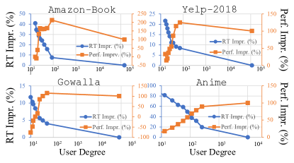
Figure 2. The performance and efficiency improvement of TAG-CF⁺ w.r.t. different cutoffs. TAG-CF⁺ further improves TAG-CF with less computational overheads. 100% is the original performance/efficiency of vanilla TAG-CF.

To answer RQ (4), we apply TAG-CF⁺ to four public datasets and the performance and the efficiency improvement are demonstrated in Figure 2. Overall, the running time improvement brought by TAG-CF⁺ exponentially increases as the degree decreases, since low-degree users have sparse neighborhoods and there is hence less information for TAG-CF⁺ to aggregation. When the degree cutoff is low (i.e., less than 100), the effectiveness of TAG-CF⁺ proportional increases as the degree cutoff increases.

When setting the cutoff to a user degree of around 100, on Amazon-Book, Gowalla, and Yelp-2018, TAG-CF⁺ can further improve TAG-CF by 125%, 17%, and 11%, respectively, with efficiency improvement of 7%, 4%, and 8%. In these cases, TAG-CF⁺ not only significantly improves the performance but also effectively reduces computational overheads. However, on these three datasets, after the cutoff bypasses a degree of 100, the performance improvement eventually decreases to the performance of TAG-CF (i.e., 100%), indicating that test-time aggregation jeopardizes the performance on high-degree nodes. On Anime, though no downgrade on high-degree users, the performance improvement of TAG-CF⁺ to TAG-CF is incremental. These phenomenons not only demonstrate the effectiveness and efficiency of TAG-CF⁺, but also verify our findings in Section 3.2 that message passing in CF helps low-degree users more than high-degree users.

Table 6. Improvement (NDCG@20) brought by TAG-CF at different degree cutoffs and upsampling rates on ML-1M.

Up-sampling	Up-sample Rate: 100%			Up-sample Rate: 300%
Degree
	MF	+ TAG-CF	Impr. ($\uparrow$%)	MF	+ TAG-CF	Impr. ($\uparrow$%)
40	20.62	28.87	38.8%	19.30	25.01	30.3%
80	20.10	27.43	35.9%	18.40	23.30	26.8%
160	19.39	26.63	36.6%	17.93	23.37	29.8%

5.6. Analysis of TAG-CF through Up-sampling

In Section 3, we connect CF objective functions to message passing and show that they inadvertently conduct message passing during the back-propagation. Since this inadvertent message passing happens during the back-propagation, its performance is positively correlated to the amount of training signals a user/item can get. In the case of CF, the amount of training signals for a user is directly proportional to the node degree of this user. High-degree active users naturally benefit more from the inadvertent message passing from objective functions like BPR and DirectAU, because they acquire more training signals from the objective function. Hence, when explicit message passing is applied to CF methods, the performance gain for high-degree users is less significant than that for low-degree users. Because the contribution of the message passing over high-degree nodes has been mostly fulfilled by the inadvertent message passing during the training.

To quantitatively prove this line of theory, we incrementally up-sample low-degree training examples and observe the performance improvement that TAG-CF could introduce at each upsampling rate. If our line of theory is correct, then we should expect less performance improvement on low-degree users for a larger upsampling rate. The results are shown in Table 6. From this table, though upsampling low-degree users hurts the overall performance, we can observe that the performance improvement brought by TAG-CF for low-degree users decreases, as the upsampling rate increases.

According to this experiment, we can conclude that the more supervision signals a user receives (no matter for a low-degree or high-degree user), the less performance improvement message passing can bring. This experiment quantitatively shows why the performance improvement of high-degree users could be limited more than low-degree users. Because high-degree users naturally receive more training signals during the training whereas low-degree users receive fewer training signals.

6. Conclusion

In this study, we investigate how message passing improves collaborative filtering. Through a series of ablations, we demonstrate that the performance gain from neighbor contents dominates that from accompanying gradients brought by message passing in CF. Moreover, for the first time, we show that message passing in CF improves low-degree users more than high-degree users. We theoretically demonstrate that CF supervision signals inadvertently conduct message passing in the backward step, even without treating the data as a graph. In light of these novel takeaways, we propose TAG-CF, a test-time aggregation framework effective at enhancing representations trained by different CF supervision signals. Evaluated on five datasets, TAG-CF performs at par with SoTA methods with only a fraction of computational overhead (i.e., less than 1.0% of the total training time).

Appendix A Proof of Theorem 1

One preliminary theoretical foundation for Theorem 1 to hold is that a K-layer graph convolution network (GCN) exactly optimizes the second term in Equation 8, which has been proved by (zhu2021interpreting, ). With this preliminary, the proof to Theorem 1 starts as:

Proof.

DirectAU optimizes:

(10) $$\mathcal{L}_{\text{DirectAU}} =\sum_{(i,j)\in\mathcal{D}}||\mathbf{u}_{i}-\mathbf{i}_{j}||^{2}$$

(11) $$+\sum_{u,u^{\prime}\in\mathcal{U}}\log e^{-2||\mathbf{u}-\mathbf{u}^{\prime}||^{2}}+\sum_{i,i^{\prime}\in\mathcal{I}}\log e^{-2||\mathbf{i}-\mathbf{i}^{\prime}||^{2}}.$$

Since $\sum_{u,u^{\prime}\in\mathcal{U}}\log e^{-2||\mathbf{u}-\mathbf{u}^{\prime}||^{2}}<=0$ and $\sum_{i,i^{\prime}\in\mathcal{I}}\log e^{-2||\mathbf{i}-\mathbf{i}^{\prime}||^{2}}<=0$, we directly have $\mathcal{L}_{\text{DirectAU}}\leq\sum_{(i,j)\in\mathcal{D}}||\mathbf{u}_{i}-\mathbf{i}_{j}||^{2}$.

BPR optimizes:

(12) $$\mathcal{L}_{\text{BPR}} =-\sum_{(i,j)\in\mathcal{D}}\sum_{(i,k)\notin\mathcal{D}}\log\sigma(s_{ij}-s_{ik})=$$

(13) $$-\sum_{(i,j)\in\mathcal{D}}\sum_{(i,k)\notin\mathcal{D}}\log\sigma(\mathbf{u}_{i}^{\intercal}\cdot\mathbf{i}_{j}-\mathbf{u}_{i}^{\intercal}\cdot\mathbf{i}_{k})$$

(14) $$=\sum_{(i,j)\in\mathcal{D}}\sum_{(i,k)\notin\mathcal{D}}-\log\Big{(}\frac{e^{\mathbf{u}_{i}^{\intercal}\cdot\mathbf{i}_{j}}}{e^{\mathbf{u}_{i}^{\intercal}\cdot\mathbf{i}_{j}}+e^{\mathbf{u}_{i}^{\intercal}\cdot\mathbf{i}_{k}}}\Big{)}$$

(15) $$=\sum_{(i,j)\in\mathcal{D}}\sum_{(i,k)\notin\mathcal{D}}-\mathbf{u}_{i}^{\intercal}\cdot\mathbf{i}_{j}+\log\Big{(}e^{\mathbf{u}_{i}^{\intercal}\cdot\mathbf{i}_{j}}+e^{\mathbf{u}_{i}^{\intercal}\cdot\mathbf{i}_{k}}\Big{)}$$

Since $||\mathbf{u}_{i}||^{2}=||\mathbf{i}_{j}||^{2}=1$ for any $u_{i}\in\mathcal{U}$ and $I_{j}\in\mathcal{I}$, $||\mathbf{u}_{i}-\mathbf{i}_{j}||=\sqrt{1-2\mathbf{u}_{i}^{\intercal}\cdot\mathbf{i}_{j}+1}\rightarrow-\mathbf{u}_{i}^{\intercal}\cdot\mathbf{i}_{j}=\frac{1}{2}||\mathbf{u}_{i}-\mathbf{i}_{j}||^{2}-1$. So Equation 15 can be written as:

(16) $$\mathcal{L}_{\text{BPR}}=\frac{1}{2}||\mathbf{u}_{i}-\mathbf{i}_{j}||^{2}-1+\log\Big{(}e^{\mathbf{u}_{i}^{\intercal}\cdot\mathbf{i}_{j}}+e^{\mathbf{u}_{i}^{\intercal}\cdot\mathbf{i}_{k}}\Big{)}.$$

The maximum possible value of $e^{\mathbf{u}_{i}^{\intercal}\cdot\mathbf{i}_{j}}+e^{\mathbf{u}_{i}^{\intercal}\cdot\mathbf{i}_{k}}$ is $2e$, which is less than 10. Hence $\log\Big{(}e^{\mathbf{u}_{i}^{\intercal}\cdot\mathbf{i}_{j}}+e^{\mathbf{u}_{i}^{\intercal}\cdot\mathbf{i}_{k}}\Big{)}<1$, which leads to the second part of Theorem 1: $\mathcal{L}_{\text{BPR}}\leq\sum_{(i,j)\in\mathcal{D}}||\mathbf{u}_{i}-\mathbf{i}_{j}||^{2}$. ∎

Appendix B Dataset Description and Statistics

We conduct experiments on five commonly used benchmark datasets, that have been broadly utilized by the recommender system community, including Amazon-book (mcauley2016addressing, ), Anime (anime, ), Gowalla (cho2011friendship, ), Yelp2018 (yelp, ), and MovieLens-1M (harper2015movielens, ). Additionally, we also evaluate our method on a large-scale industrial user-content recommendation dataset - Internal, with statistics shown in Table 7.

Appendix C Additional Experimental Settings

Evaluation Protocol. We evaluate all models using metrics adopted in previous works, including NDCG@20 and Recall@20 (he2020lightgcn, ). For the dataset split, we conduct the group-by-user splits and randomly select 80%, 10%, and 10% of observed interactions as training, validation, and testing sets respectively. We adopt an early stopping strategy, where the training will be terminated if the validation NDCG@20 stops increasing for 3 continuous epochs.

Hyper-parameter Tuning We only conduct 25 searches per model for all methods to ensure the comparison fairness, so that our experiments are not biased to methods with sophisticated hyper-parameter search spaces. Furthermore, we set the embedding dimensions for all models to 64 (i.e., $d=64$) to ensure a fair comparison, since a larger dimension usually leads to better performance in CF methods. For TAG-CF, we only tune $m$ and $n$ in Equation 9 during test time from the list of [-2, -1.5, -1, -0.5, 0].

Implementation Detail We conduct most of the baseline experiments with RecBole (zhao2022recbole, ). Besides, we use Google Cloud Platform with 12 CPU cores, 64GB RAM, and a single V100 GPU with 16GB VRAM to run all experiments.

Table 7. Dataset Statistics. Due to privacy constrains, we only report approximated values for Internal dataset.

Dataset	# Users	# Items	# Interactions	Sparsity
Amazon-book	52,643	40,981	2,984,108	99.94%
Anime	73,515	12,295	7,813,727	99.13%
Gowalla	29,858	40,981	1,027,370	99.91%
Yelp-2018	31,668	38,048	1,561,406	99.87%
MovieLens-1M	6,040	3,629	836,478	96.18%
Internal	$\sim$0.5M	$\sim$0.2M	$\sim$7M	99.99%

Table 8. Improvement of TAG-CF⁺ to TAG-CF. Degree cutoffs are selected according to Figure 3.

Metric	Yelp-2018	Gowalla	Amazon-book	Anime
BPR
NDCG@20	27.1%	10.3%	122.4%	0%
Recall@20	31.4%	14.2%	119.2%	0%
Running Time	8%	4%	9%	0%
DirectAU
NDCG@20	34.1%	22.5%	98.3%	0%
Recall@20	29.2%	30.1%	104.1%	0%
Running Time	8%	4%	9%	0%

Appendix D Degree Cutoff Selection for TAG-CF⁺

We first sort all users according to their degree and split the sorted list into 10 user buckets, where each bucket contains non-overlapped users with similar degrees. Starting from the bucket with the lowest user degree, TAG-CF⁺ keeps applying test-time-aggregation demonstrated in Equation 9 to all buckets until the validation performance starts to decrease or the performance improvement is less than $2\%$ compared with TAG-CF. The degree cutoffs circled in Figure 3 are the ones selected by this strategy and most of them correspond to the most performant configuration, shown in Table 8.

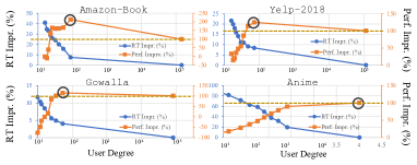
Figure 3. Improvement of TAG-CF⁺ w.r.t. different cutoffs. Yellow dashed lines indicate TAG-CF, and black circles refer to the optimal degree cutoff that TAG-CF⁺ selects.

References

- (1) Cai, X., Huang, C., Xia, L., and Ren, X. Lightgcl: Simple yet effective graph contrastive learning for recommendation. In Procs. of ICLR (2023).
- (2) Chang, J., Gao, C., Zheng, Y., Hui, Y., Niu, Y., Song, Y., Jin, D., and Li, Y. Sequential recommendation with graph neural networks. In Procs. of SIGIR (2021).
- (3) Chen, C., Zhang, M., Zhang, Y., Liu, Y., and Ma, S. Efficient neural matrix factorization without sampling for recommendation. ACM Transactions on Information Systems (TOIS) (2020).
- (4) Chen, J., Dong, H., Wang, X., Feng, F., Wang, M., and He, X. Bias and debias in recommender system: A survey and future directions. ACM Transactions on Information Systems 41, 3 (2023), 1–39.
- (5) Cho, E., Myers, S. A., and Leskovec, J. Friendship and mobility: user movement in location-based social networks. In Procs of SIGKDD (2011).
- (6) Dasoulas, G., Lutzeyer, J. F., and Vazirgiannis, M. Learning parametrised graph shift operators. In Procs of ICLR (2021).
- (7) Dong, X., Thanou, D., Frossard, P., and Vandergheynst, P. Learning laplacian matrix in smooth graph signal representations. IEEE Transactions on Signal Processing (2016).
- (8) Dong, X., Thanou, D., Rabbat, M., and Frossard, P. Learning graphs from data: A signal representation perspective. IEEE Signal Processing Magazine (2019).
- (9) Fan, Y., Ju, M., Zhang, C., and Ye, Y. Heterogeneous temporal graph neural network. In Procs. of SDM (2022).
- (10) Gao, C., Wang, X., He, X., and Li, Y. Graph neural networks for recommender system. In Procs. of WSDM (2022).
- (11) Gao, C., Zheng, Y., Li, N., Li, Y., Qin, Y., Piao, J., Quan, Y., Chang, J., Jin, D., He, X., et al. A survey of graph neural networks for recommender systems: Challenges, methods, and directions. ACM Transactions on Recommender Systems (2023).
- (12) Gilmer, J., Schoenholz, S. S., Riley, P. F., Vinyals, O., and Dahl, G. E. Neural message passing for quantum chemistry. In Procs. of ICML (2017).
- (13) Gomez-Uribe, C. A., and Hunt, N. The netflix recommender system: Algorithms, business value, and innovation. ACM Transactions on Management Information Systems (TMIS) (2015).
- (14) Guo, Z., Shiao, W., Zhang, S., Liu, Y., Chawla, N. V., Shah, N., and Zhao, T. Linkless link prediction via relational distillation. In International Conference on Machine Learning (2023), PMLR, pp. 12012–12033.
- (15) Guo, Z., Zhao, T., Liu, Y., Dong, K., Shiao, W., Shah, N., and Chawla, N. V. Node duplication improves cold-start link prediction. arXiv preprint arXiv:2402.09711 (2024).
- (16) Hamilton, W. L., Ying, R., and Leskovec, J. Inductive representation learning on large graphs. In Procs. of NeurIPS (2017).
- (17) Harper, F. M., and Konstan, J. A. The movielens datasets: History and context. Acm transactions on interactive intelligent systems (tiis) (2015).
- (18) He, X., Deng, K., Wang, X., Li, Y., Zhang, Y., and Wang, M. Lightgcn: Simplifying and powering graph convolution network for recommendation. In Procs. of SIGIR (2020).
- (19) He, X., Liao, L., Zhang, H., Nie, L., Hu, X., and Chua, T.-S. Neural collaborative filtering. In Procs. of WWW (2017).
- (20) Hu, W., Cao, K., Huang, K., Huang, E. W., Subbian, K., and Leskovec, J. Tuneup: A training strategy for improving generalization of graph neural networks. arXiv (2022).
- (21) Ju, M., Fan, Y., Zhang, C., and Ye, Y. Let graph be the go board: gradient-free node injection attack for graph neural networks via reinforcement learning. In Procs. of AAAI (2023).
- (22) Ju, M., Zhao, T., Wen, Q., Yu, W., Shah, N., Ye, Y., and Zhang, C. Multi-task self-supervised graph neural networks enable stronger task generalization. In Procs. of ICLR (2023).
- (23) Ju, M., Zhao, T., Yu, W., Shah, N., and Ye, Y. Graphpatcher: Mitigating degree bias for graph neural networks via test-time augmentation. In Procs. of NeurIPS (2023).
- (24) Kaggle. Anime Recommendatiosn Database. https://www.kaggle.com/datasets/CooperUnion/anime-recommendations-database, 2023. [Online; accessed June-2023].
- (25) Kipf, T. N., and Welling, M. Semi-supervised classification with graph convolutional networks. In Procs. of ICLR (2016).
- (26) Koren, Y., Bell, R., and Volinsky, C. Matrix factorization techniques for recommender systems. Computer (2009).
- (27) Koren, Y., Rendle, S., and Bell, R. Advances in collaborative filtering. Recommender systems handbook (2021), 91–142.
- (28) Lin, Z., Tian, C., Hou, Y., and Zhao, W. X. Improving graph collaborative filtering with neighborhood-enriched contrastive learning. In Procs of WWW (2022).
- (29) Liu, Z., Nguyen, T.-K., and Fang, Y. Tail-gnn: Tail-node graph neural networks. In Procs. of SIGKDD (2021).
- (30) Ma, Y., Liu, X., Shah, N., and Tang, J. Is homophily a necessity for graph neural networks? In Procs. of ICLR (2022).
- (31) Ma, Y., Liu, X., Zhao, T., Liu, Y., Tang, J., and Shah, N. A unified view on graph neural networks as graph signal denoising. In Proceedings of the 30th ACM International Conference on Information & Knowledge Management (2021), pp. 1202–1211.
- (32) Mao, K., Zhu, J., Xiao, X., Lu, B., Wang, Z., and He, X. Ultragcn: ultra simplification of graph convolutional networks for recommendation. In Procs. of CIKM (2021).
- (33) McAuley, J., and Yang, A. Addressing complex and subjective product-related queries with customer reviews. In Procs. of WWW (2016).
- (34) Oloulade, B. M., Gao, J., Chen, J., Lyu, T., and Al-Sabri, R. Graph neural architecture search: A survey. Tsinghua Science and Technology (2021).
- (35) Pal, A., Eksombatchai, C., Zhou, Y., Zhao, B., Rosenberg, C., and Leskovec, J. Pinnersage: Multi-modal user embedding framework for recommendations at pinterest. In Procs. of SIGKDD (2020).
- (36) Peng, S., Sugiyama, K., and Mine, T. Svd-gcn: A simplified graph convolution paradigm for recommendation. In Procs of CIKM (2022).
- (37) Rendle, S., Freudenthaler, C., Gantner, Z., and Schmidt-Thieme, L. Bpr: Bayesian personalized ranking from implicit feedback. In UAI (2009).
- (38) Sankar, A., Liu, Y., Yu, J., and Shah, N. Graph neural networks for friend ranking in large-scale social platforms. In Proceedings of the Web Conference 2021 (2021), pp. 2535–2546.
- (39) Schafer, J. B., Konstan, J., and Riedl, J. Recommender systems in e-commerce. In Procs. of ACM conference on Electronic commerce (1999).
- (40) Shen, Y., Wu, Y., Zhang, Y., Shan, C., Zhang, J., Letaief, B. K., and Li, D. How powerful is graph convolution for recommendation? In Procs. of CIKM (2021).
- (41) Shi, J., Ji, H., Shi, C., Wang, X., Zhang, Z., and Zhou, J. Heterogeneous graph neural network for recommendation. arXiv preprint arXiv:2009.00799 (2020).
- (42) Su, X., and Khoshgoftaar, T. M. A survey of collaborative filtering techniques. Advances in artificial intelligence (2009).
- (43) Tang, X., Yao, H., Sun, Y., Wang, Y., Tang, J., Aggarwal, C., Mitra, P., and Wang, S. Investigating and mitigating degree-related biases in graph convoltuional networks. In Procs. of CIKM (2020).
- (44) Van den Oord, A., Dieleman, S., and Schrauwen, B. Deep content-based music recommendation. In Procs. of NeurIPS (2013).
- (45) Veličković, P., Cucurull, G., Casanova, A., Romero, A., Lio, P., and Bengio, Y. Graph attention networks. In Procs. of ICLR (2017).
- (46) Wang, C., Yu, Y., Ma, W., Zhang, M., Chen, C., Liu, Y., and Ma, S. Towards representation alignment and uniformity in collaborative filtering. In Procs. of SIGKDD (2022).
- (47) Wang, H., Wang, N., and Yeung, D.-Y. Collaborative deep learning for recommender systems. In Procs. of SIGKDD (2015).
- (48) Wang, R., Shivanna, R., Cheng, D., Jain, S., Lin, D., Hong, L., and Chi, E. Dcn v2: Improved deep & cross network and practical lessons for web-scale learning to rank systems. In Procs. of WWW (2021).
- (49) Wang, X., He, X., Wang, M., Feng, F., and Chua, T.-S. Neural graph collaborative filtering. In Procs. of SIGIR (2019).
- (50) Wang, X., Jin, H., Zhang, A., He, X., Xu, T., and Chua, T.-S. Disentangled graph collaborative filtering. In Procs. of SIGIR (2020).
- (51) Wang, Y., Jin, J., Zhang, W., Yu, Y., Zhang, Z., and Wipf, D. Bag of tricks for node classification with graph neural networks. arXiv preprint arXiv:2103.13355 (2021).
- (52) Wei, Y., Wang, X., Li, Q., Nie, L., Li, Y., Li, X., and Chua, T.-S. Contrastive learning for cold-start recommendation. In Proceedings of the 29th ACM International Conference on Multimedia (2021), pp. 5382–5390.
- (53) Wu, J., Wang, X., Feng, F., He, X., Chen, L., Lian, J., and Xie, X. Self-supervised graph learning for recommendation. In Procs. of SIGIR (2021).
- (54) Wu, S., Sun, F., Zhang, W., Xie, X., and Cui, B. Graph neural networks in recommender systems: a survey. ACM Computing Surveys 55, 5 (2022), 1–37.
- (55) Xia, L., Huang, C., Shi, J., and Xu, Y. Graph-less collaborative filtering. In Procs. of WWW (2023).
- (56) Xia, L., Xu, Y., Huang, C., Dai, P., and Bo, L. Graph meta network for multi-behavior recommendation. In Procs. of SIGIR (2021).
- (57) Xu, K., Hu, W., Leskovec, J., and Jegelka, S. How powerful are graph neural networks? In Procs. of ICLR (2018).
- (58) Xu, K., Li, C., Tian, Y., Sonobe, T., Kawarabayashi, K.-i., and Jegelka, S. Representation learning on graphs with jumping knowledge networks. In Procs. of ICML (2018).
- (59) Yelp. Yelp Open Dataset. https://www.yelp.com/dataset, 2023. [Online; accessed June-2023].
- (60) Ying, R., He, R., Chen, K., Eksombatchai, P., Hamilton, W. L., and Leskovec, J. Graph convolutional neural networks for web-scale recommender systems. In Procs. of SIGKDD (2018).
- (61) Yu, J., Yin, H., Li, J., Wang, Q., Hung, N. Q. V., and Zhang, X. Self-supervised multi-channel hypergraph convolutional network for social recommendation. In Procs. of WWW (2021).
- (62) Yu, J., Yin, H., Xia, X., Chen, T., Cui, L., and Nguyen, Q. V. H. Are graph augmentations necessary? simple graph contrastive learning for recommendation. In Procs. of SIGIR (2022).
- (63) Zeng, H., Zhang, M., Xia, Y., Srivastava, A., Malevich, A., Kannan, R., Prasanna, V., Jin, L., and Chen, R. Decoupling the depth and scope of graph neural networks. Advances in Neural Information Processing Systems 34 (2021), 19665–19679.
- (64) Zhang, S., Liu, Y., Sun, Y., and Shah, N. Graph-less neural networks: Teaching old mlps new tricks via distillation. arXiv preprint arXiv:2110.08727 (2021).
- (65) Zhang, S., Yao, L., Sun, A., and Tay, Y. Deep learning based recommender system: A survey and new perspectives. ACM computing surveys (CSUR) (2019).
- (66) Zhao, W. X., Hou, Y., Pan, X., Yang, C., Zhang, Z., Lin, Z., Zhang, J., Bian, S., Tang, J., Sun, W., et al. Recbole 2.0: towards a more up-to-date recommendation library. In Procs. of CIKM (2022).
- (67) Zhu, M., Wang, X., Shi, C., Ji, H., and Cui, P. Interpreting and unifying graph neural networks with an optimization framework. In Procs. of WWW (2021).