1]\orgdivLaboratoire de Mécanique des Solides (LMS), \orgnameÉcole Polytechnique, Institut Polytechnique de Paris, CNRS UMR 7649, \orgaddress\streetRoute de Saclay, \postcode91120, \cityPalaiseau, \countryFrance
2]\orgdivSchool of Physics and Astronomy, \orgnameUniversity of Minnesota, \orgaddress\street116 Church St. SE, \cityMinneapolis, \postcode55455, \stateMinnesota, \countryUSA
Coupling Phase Field Crystal and Field Dislocation Mechanics for a consistent description of dislocation structure and elasticity
Abstract
This work addresses differences in predicted elastic fields created by dislocations either by the Phase Field Crystal (PFC) model, or by static Field Dislocation Mechanics (FDM). The PFC order parameter describes the topological content of the lattice, but it fails to correctly capture the elastic distortion. In contrast, static FDM correctly captures the latter but requires input about defect cores. The case of a dislocation dipole in two dimensional, isotropic, elastic medium is studied, and a weak coupling is introduced between the two models. The PFC model produces compact and stable dislocation cores, free of any singularity, i.e., diffuse. The PFC predicted dislocation density field (a measure of the topological defect content) is used as the source (input) for the static FDM problem. This coupling allows a critical analysis of the relative role played by configurational (from PFC) and elastic (from static FDM) fields in the theory, and of the consequences of the lack of elastic relaxation in the diffusive evolution of the PFC order parameter.
keywords:
dislocations, elasticity, phase field, stresses, distortions1 Introduction
Research on the motion of individual or a small number of dislocations at the nanoscale is motivated by ongoing advances in diagnostic techniques, for example, high energy X-ray and Bragg coherent diffractive imaging, that have opened the door to detailed nanoscale observation of crystalline defects such as dislocations (line-type defects) [1, 2, 3, 4, 5] and of emergent, collective mesoscale phenomena [6, 7, 8]. Combining this information with nanoscale theory and computation is key to understanding materials response, performance, and evolution across different length scales.
Field dislocation mechanics (FDM) [9, 10, 11, 12, 13, 14, 15, 16, 17] and phase field crystal models (PFC) [18, 19, 20] are two widely used approaches to study the nanoscale response of crystals containing dislocations [21, 22, 23]. Since fast temporal scales associated with lattice vibration are eliminated in both theories, their computational implementation can efficiently access long time phenomena that are difficult to describe by other methods operating at similar length scales such as molecular dynamics [24, 25].
FDM is a continuum theory [9, 10, 11, 13, 14, 15, 26, 27, 28] in which thermal lattice vibration is not considered. Rather, the theory focuses on the longer time scale of dislocation motion and chooses as a primary field the polar dislocation density tensor and its associated conservation law of topological charge [29, 30, 14, 31]. The theory also includes nonlinear, anisotropic elastic fields, and therefore it can account for topological defects in atomic configurations of nonlinear elastic media. The fundamental equations of the theory are directly derived from classical balances of mass and momentum, an elastic incompatibility equation linking the finite elastic distortion to the dislocation density tensor, and a conservation law for Burgers vector in the body. An energy dissipation inequality based on the Second Law leads to the equations for the various fields [27, 28]. Recently, the theory was extended to account for the role of thermal strain incompatibilities on the conservation of Burgers vector and temperature evolution due to dislocation activity through the first law of thermodynamics [32, 33]. The FDM theory requires some minimal, but essential constitutive input: The mobility law of single defects, and its constitutive nonlinear (and non-monotone) elastic behavior (i.e., nonlinear elasticity and appropriate generalized stacking fault energies [34, 35, 36]). Nevertheless, the theory does not require slip systems to be known a priori in order to define an energy density. Importantly, the dissipation inequality yields the proper nonlinear generalization of the Peach-Koehler force field acting on a dislocation segment.
The PFC model introduces a phase field that describes the temporally coarse grained atomic density of the crystal, and a phenomenologically specified free energy functional determined by lattice symmetry. By construction, the minimizer of the free energy is a spatially periodic phase field of the required symmetry [20]. Dissipative evolution of the phase field is assumed as a gradient flow driven by the same free energy functional. Prior research has considered both equilibrium properties, such as elastic constants [37], as well as many features of inhomogeneous systems such as, for example, dislocation motion [38, 39, 40, 41] and grain boundary structure and motion [37, 42, 43]. Since the configuration of the system is described by a single scalar field, the simultaneous description of mass density and crystalline lattice with the same order parameter constitutes an overspecified problem. This has been addressed by the introduction of a dissipative current associated with an independent vacancy diffusion mode in [44] (see, also, [45] for further discussion). This separation, however, is not sufficient to describe the motion of topological defects in which the difference between mass and lattice velocities has topological content [46, 29, 45]. Such a separation has been recently introduced in the PFC by assuming that the phase field order parameter determines only the transverse/incompatible part of the elastic distortion tensor, with the longitudinal/compatible part remaining free to capture compatible lattice distortion, and satisfy elastic equilibrium [39, 40]. However, the evolution equation for the phase field was modified in an ad hoc fashion to include an affine distortion derived from the compatible distortion.
A theory that is free of the limitations described above, and that couples FDM and the PFC, was proposed in [47]. The general approach is motivated by the great success of the Peierls model in elucidating basic dislocation physics, while the theory adds a consistent scheme for regularizing stress fields near dislocation cores. It borrows from the PFC model its definition of the order parameter and the associated free energy functional. This field naturally incorporates defect cores, which are kept localized and compact by its free energy, and features dissipative motion while preserving topological charge. All topological features of defects are maintained by the phase field evolution, which are solely dictated by the symmetry of the lattice (without any consideration of elastic interactions). The topological content of the PFC is then coupled to an elastic material described within finite deformation FDM theory. Elasticity is coupled back to the evolution of the phase field through consideration of a dissipation inequality for the full model.
However, a computational implementation of the coupled PFC and FDM model is lacking. As a first step, in this work, we propose an algorithm for a weakly coupled version of this theory within a small deformation framework. The numerical implementation is used to determine the equilibrium configuration of a dislocation dipole in two dimensions and in an elastically isotropic system. The aim of this study is to determine to what extent the PFC and FDM predicted distortions and stresses agree in equilibrium.
2 Coupled Phase Field Crystal and static Field Dislocation Mechanics
We focus on an analysis of the equilibrium configuration of a dislocation dipole in a two dimensional hexagonal lattice, in the small deformation approximation, starting from a weakly coupled formulation of the theory proposed in [47].
2.1 Phase Field Crystal
The PFC model is described by a single scalar order parameter , which is a function of position and time . The governing phenomenological free energy functional (in dimensionless form) is given by [48]
| (1) |
where is a dimensionless parameter. For , the minimizer is . For there is a continuum band of periodic solutions with either uniaxial or hexagonal symmetry of characteristic wavenumber . The amplitude of is proportional to for small . The symmetry of the minimizer depends on the value of
| (2) |
where is the surface area of the system. We focus here on and values of that correspond to a stable hexagonal phase [48]. To lowest order in (the “single mode approximation”), the minimizer is approximately given by,
| (3) |
with , , , , and [20]
| (4) |
The vectors are the Cartesian unit vectors. This solution is approximate up to , with the next order being . However, it is common practice in numerical work involving the PFC model to consider values of that are . Higher order terms in missing in Eq. (3) don’t seem to appreciably modify long wavelength modulation of . Indeed, the numerical solution for used below does contain the entire sequence of perturbative terms, though the decomposition involving complex amplitudes in Eqs. (3) and (6) is only approximate. In the small deformation limit, the energy of an elastic distortion of Eq. (1) is isotropic, with the Lamé coefficients given by [39].
The temporal evolution of is defined as a (nonconserved) -gradient flow
| (5) |
In order to maintain the value of fixed during the evolution of , we explicitly impose Eq. (2) as a global constraint. This procedure differs from the more conventional approach of rewriting Eq. (5) as a flow locally conserving (“conserved order parameter”). The variational analysis of [47] applies only to the nonconserved case, Eq. (5). It would have to be generalized to the locally conserved case if a conserved order parameter model were to be chosen. However, in that case the evolution equation for the order parameter contains two additional orders in derivatives of , and we see no physical reason to justify the added complexity.
A key tenet of the theory in [47] is that the coupling between order parameter configurational distortion and material elastic distortion takes place only over scales that are large compared with the (microscopic) order parameter wavelength. There is no reason to believe that elastic distortion and elastic energies could be meaningfully defined at the microscopic scale of the PFC model. As a first step a slowly varying configurational distortion is introduced in a standard way thorough a multiple scale expansion of the order parameter [49] as follows:
| (6) |
where it is understood that the variation of on its arguments is slow in a multiple scale expansion sense. From a numerical perspective, the slowly varying amplitudes will be computed below by a local demodulation of the phase field as
| (7) |
obtained through the convolution with a two-dimensional Gaussian kernel of width on the order of the lattice parameter of the phase field,
| (8) |
With this definition, the configurational distortion tensor of the phase field, , is defined as [39]
| (9) |
where is the dimension of the system, is the imaginary part of the complex number , and for a hexagonal lattice in two dimensions [41]. The tensor has the same symmetry properties under rotation as the elastic distortion (from FDM), is a functional at each point of the phase field , and is defined so as to capture the slowly varying distortion of surfaces of constant . Therefore this tensor describes a local configurational distortion of the phase field, without endowing it with any elastic properties.
In analogy with linear elasticity, a configurational stress tensor can be defined as
| (10) |
where plays the role of a stiffness tensor. In the isotropic elastic case it is given as .
It is also possible to define a configurational stress by directly computing the variation of the phase field free energy to an affine distortion , with as [39]
| (11) |
where the free energy density is defined in Eq. (1), and is the rank two identity tensor. A slowly varying configurational stress can be defined by demodulation as . While both and are linear in the distortion , the former is a variation relative to a possibly distorted reference configuration whereas the latter is a variation relative to the undistorted ground state. Therefore, they are expected to coincide in weakly distorted regions such as far from dislocation cores, but are expected to differ in the vicinity of defects.
The PFC order parameter supports not only smooth distortions but also isolated, topologically stable, dislocations. They have been extensively studied for two dimensional uniaxial and hexagonal patterns of fluid convection [50, 49, 51, 52]. For defected crystalline materials, they have been analyzed in [39] in two dimensions, and in [41] in three dimensions. A dislocation in a configuration of at corresponds to a nonzero around a contour containing only that dislocation. The corresponding distortion of the phase field leads to , with non singular and . Defining a topological charge as , , so that a dislocation at corresponds to vortices in the complex amplitude , of winding number . Note that . Therefore, in two dimensions, a phase field dislocation comprises vortices in two of the complex amplitudes (), whereas the third is non singular ().
This nonzero circulation can be transformed into an area integral, leading to the definition of the phase field dislocation density tensor,
| (12) |
Although the tensor can be explicitly written in terms of [41], in our calculations below we will first determine from the phase field amplitudes, Eq. (9), and then directly from Eq. (12).
2.2 Field Dislocation Mechanics
In the static setting within a small deformation framework, FDM takes as input a polar dislocation density field , and mechanical boundary conditions, and yields the elastic distortion field and the stress field . The latter is related to the former through the Hooke’s law as
| (13) |
In a simply connected domain with no dislocations, the elastic distortion field is compatible, such that (see Appendix A for notation). If a simply connected two-dimensional domain has a distribution of ‘’ point dislocations of Burgers vectors , the elastic distortion is related to the Burgers vector as , where the contour over which the integral is taken encloses only the dislocation. The inequality holds only when the elastic distortion field has an incompatible/transverse component i.e., a component with a non-zero curl. The static FDM model starts from a Stokes-Helmholtz type decomposition of a tensor to uniquely express the elastic distortion field into compatible/longitudinal (curl free) and incompatible/transverse (divergence free) components as , such that . In small deformation, the polar dislocation density field is defined as . Then, for a given field, can be obtained by solving the following Poisson-type equation
| (14) |
2.3 Weak coupling
We want to examine the equilibrium configuration of a defected medium comprising a stationary dislocation dipole under periodic boundary conditions. An initial configuration comprising a dislocation dipole is considered in a climb configuration. For values of , the order parameter relaxes everywhere according to Eq. (5), but the location of the dislocation cores remains constant for very long times due to Periels barriers to motion [52]. Therefore, at long times, the field is a constrained minimizer of given the location and Burgers vectors of the two dislocations. The phase field is used to compute (Eq. (12)). Next we set and solve the resulting static FDM problem for an elastic medium under periodic boundary conditions. The restricted assumption that the static FDM and the PFC only couple through the dislocation density tensor implies that the incompatible part is equal to the incompatible part of . However, importantly, the compatible part of i.e., , is not equal to the compatible part of . Determination of requires the resolution of equation (15).
3 Algorithm and numerical implementation
A uniform spatial grid is introduced in a rectangular domain with points along and along . The grid spacing is , with as dictated by the hexagonal ground state of the free energy in Eq. (1). The lateral size of the domain along and is and , respectively (Figure 1a) as we assume periodic boundary conditions along both directions. Given these boundary conditions, Fourier transforms of the variables are introduced. Spatial derivatives are computed by either their spectral representation or by central finite differences, whereas time discretization is performed using a forward Euler scheme.
The initial condition for the order parameter includes dislocations at ,
| (18) |
with computed using Eq. (4). For the current time step , with all the quantities known at the previous time step , the PFC problem is iterated first according to,
| (19) |
where is the linear operator of Eq. (5) acting on , is the time step, and quantities with superscript refer to the previous time step. The first term on the right hand side of Eq. (19), can be rewritten as an approximation of , where , and is the wavevector in Fourier space. The symbol stands for Fourier transform, and a tilde over a variable denotes its Fourier transform. For better accuracy, the expression involving the exponential function in Fourier space is used. Only wavenumbers are considered so that the first term in Eq. (19) is computed as,
| (20) |
with
| (21) |
where and are user-defined constants.
Finally, is computed as
| (22) |
Once has been obtained, it is used to find using,
| (23) |
which in turn is used to compute using the central difference approximation to Eq. (9). Then, is straightforwardly obtained using Eq. (10). The stress is obtained by first computing and then computing
| (24) |
Next, is computed using and Eq. (12). The result is assigned to , and the elastic problem under periodic boundary conditions is solved as follows: We obtain from (14) using the Fourier transform as
| (25) |
where is defined in Appendix A. Then
| (26) |
where is the fourth order modified Green’s tensor with components in Fourier space given by
| (27) |
The stress is then straightforwardly obtained from (13) using .
Note that the mean values of both and are undefined. We set their Fourier amplitudes at to be zero as appropriate for a system with periodic boundary conditions. In order to facilitate comparison with and , we also set the mean values of the configurational stresses to be zero.
The step by step algorithm is summarized in Table 1, which has been implemented in Fortran90. The FFTW 3 [55] C++ library is used to perform forward and inverse Fourier transforms. In Fourier space, derivatives (in real space) are approximated using the central difference approach [56, 57].
4 Results
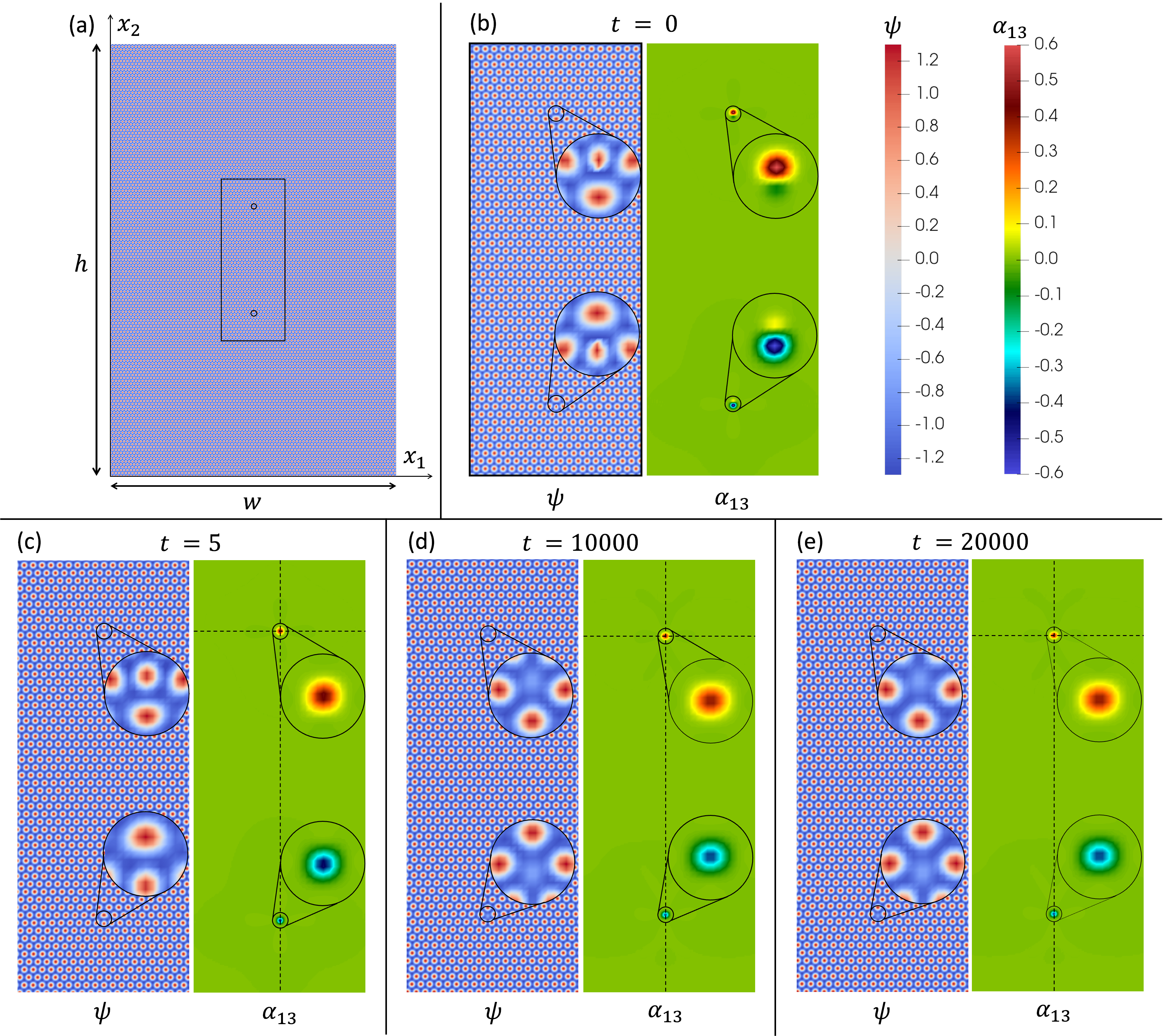
We have used points along and along , and the parameter values , well inside the hexagonal region of the phase diagram of the phase field. As initial condition, two dislocations are introduced along the line according to equation (18) with Burgers vectors at (top), and at (bottom), as shown in Figure 1b.
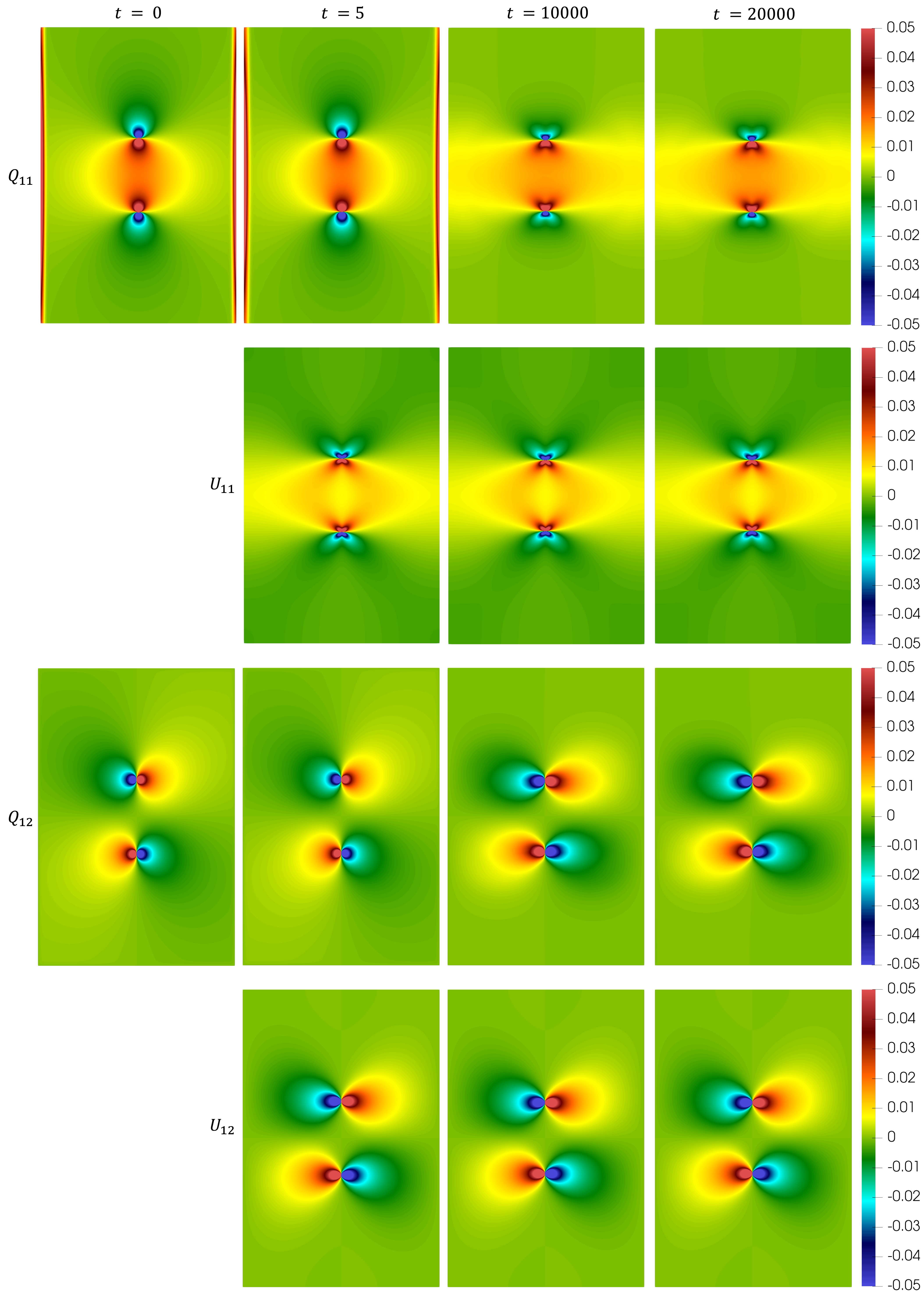
With this initial configuration, the only non zero component of the polar dislocation density is . The top and bottom dislocations should respectively exhibit and . Figure 1 shows the temporal evolution of and as the system relaxes from the initial condition. The order parameter reaches a steady state around , therefore, only results up to this time are shown. However, and as expected from the diffusive nature of the relaxation of the order parameter, reaches a time independent distribution much earlier ( in the figure). As a consequence, the contour lines of do not change or move significantly from this time until the end of the integration (Figure 2) despite the fact that continues to evolve. Indeed, after relaxation, the top and bottom dislocations respectively exhibit and .
Even though becomes time independent as early as , there are clear qualitative and quantitative differences between the spatial distributions of the corresponding components of and (Figure 2). These differences are most pronounced in the case of and . The former shows fourfold symmetry, which is the expected symmetry of this component of the elastic distortion for an edge dislocation with as the only non zero component. Meanwhile, shows a twofold geometry, which does not conform with the predictions of the elasto-static theory of dislocations i.e., static FDM. The differences are less pronounced in the case of and , nevertheless, they do exist, as evidenced in figure 2.
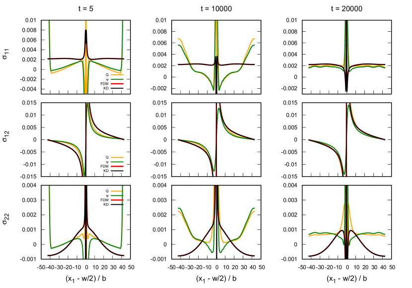
Next, a comparison is performed between the static FDM and PFC stress measures. Note that following Algorithm 1, and in order to facilitate comparison between the individual components of all the stress measures, their values have been normalized in such a way that their average over the computational domain is equal to zero. In other words, their zeroth wavenumber () component in Fourier space have been set to 0. We show comparisons of elastic and configurational stresses along two orthogonal lines in the system in Figs. 3 and 4. The various quantities plotted are along the vertical and horizontal lines shown in Figure 1, passing through the two dislocations and the top dislocation, respectively. Analogous plots comparing and lead to the same conclusions and are not been shown here.

Both figures show that the stress fields and are identical to numerical accuracy, as expected. This agreement serves as validation of the numerical algorithm and the numerical scheme based on the dislocation density as a source (input) in static FDM.
Figure 3 shows all the components of all the stress measures along . Along this line, the only non negligible components are the normal stress components; the shear stress is very small, and we do not attach any significance to any discrepancies in Figure 3. At early times (), and do not agree with anywhere along the line. The components and show better agreement with . Of course, the components of do not change significantly after (negligible changes occur due to slight movement of the dislocation cores), while the configurational stresses continue to relax. At long times ( and beyond), the system has reached a steady state. Far field configurational and elastic stresses coincide, however, they do not coincide in the region in between the dislocations. This near-field discrepancy is to be expected for several reasons. First, the core size in dimensionless units is on the order of (Fig. 1) which is not much smaller than the distance between dislocations (). Second, the phase field free energy is fully nonlinear, while the elastic stress has been obtained under the assumption of linear elasticity. Regions of large distortion will therefore have different stress distributions at equilibrium. Nevertheless, all stresses coincide far from the defect core region, thus validating the use of the PFC method to provide physically correct equilibrium values of elastic fields.
Similar conclusions can be drawn from an analysis of the stresses , and along (shown in Fig. 4). The shear stress is not negligible along this direction, with the figure showing good agreement between configurational and elastic stresses. There is some disagreement at early times (see ) because the elastic field is in equilibrium after the dislocation core has stabilized, but the phase field requires a much longer time to relax since it is doing so diffusively. At later times, however, the agreement between all the stresses is excellent. In addition to the origin of any discrepancies indicated above, the results along this direction are further affected by tensile strains at the edges of the domain; and deviate significantly from the far field equilibrium solution at all times. This is a consequence of the choice of periodic boundary conditions in a system with a small number of defects, and on the initial condition for the order parameter chosen to include two dislocations. The arctangent operator in equation (18) is clearly not compatible with periodic boundary conditions. Both effects would not be so prominent in a more complex calculation involving an ensemble of defects. In addition, since the values at of the various stress fields have been set to zero, their magnitudes in the core region affect the large distance asymptotic values when enforcing this constraint. This problem manifests in the results along but it does not manifest in the results along due to the different symmetry of the stress field.
5 Discussion and conclusions
A (weakly) coupled model involving the PFC (Phase Field Crystal) and the static FDM (Field Dislocation Mechanics) approaches has been introduced to obtain the constrained equilibrium state of a prototypical configuration involving a dislocation dipole. This configuration allows a critical analysis of the relative role played by configurational (from PFC) and elastic (from static FDM) fields in the coupled theory, the study of the consequences of introducing a consistent separation between diffusive and elastic time scales, and consideration of singularity regularization at defect cores.
The ulterior goal of this study is to endow the PFC model with material elasticity in a way that consistently respects the required independence between the order parameter and lattice distortion. We have adopted the view that the PFC order parameter only describes the topological content of the lattice, and that therefore, in equilibrium, it only determines the transverse/incompatible part of the distortion (as required by lattice incompatibility in the elastic problem). This choice leverages the fact that the PFC produces a compact and stable defect core, free of any singularity. We then use the resulting (diffuse) dislocation density in the core region as the source for the elastic problem.
Our results show that local relaxation of the order parameter at the defect core is fast, and therefore elastic equilibrium should be established rather quickly over the entire system, as shown by the resolution of the elastostatic problem. However, the configurational stresses have not been equilibrated in the early stages of the numerical calculation. It takes a long time for them to reach equilibrium because the phase field order parameter relaxes diffusively everywhere. This diffusive relaxation is unphysical for an elastic medium, and it has hindered the applicability of the PFC model to realistic elastic materials.
At much later times, the configurational stresses converge to the elasto-static solution at far field, indicating attainment of equilibrium. Any discrepancies remaining are due to the finite size of the computational domain and periodic boundary conditions. Near dislocation cores, deviations are found between the elastic and configurational stresses, which are related to the fact that the PFC model is defined by a nonlinear free energy, whereas linear elasticity has been assumed for the static FDM response.
In summary, the PFC provides a consistent method to introduce lattice incompatibility into a classical elasticity calculation in a defected medium. It remains to be investigated whether the same coupled theory provides a proper and efficient description of plastic defect motion as described in [47]. The algorithm presented in this work will provide the starting point in such an analysis. In addition to the proper separation of order parmameter and elastic time scales, attention has to be paid to a proper separation of dissipative contributions to dislocation motion of phase field and mechanical origin.
Supplementary information
Acknowledgments We are indebted to Amit Acharya for many useful and stimulating discussions. MVU is grateful to the European Research Council (ERC) for their support through the European Union’s Horizon 2020 research and innovation program for project GAMMA (Grant agreement No. 946959). The research of JV has been supported by the National Science Foundation under contract DMR-2223707.
Declarations
The authors declare no conflict of interest associated with this work.
Appendix A Definitions and notation
Scalars are denoted with an italic font (e.g., or ). Vectors are denoted by a lowercase bold and italic font (e.g., ). Unit vectors are identified by an additional overhead hat symbol e.g., . Second-order tensors are denoted by an uppercase bold and italic font or by bold and italic Greek letters (e.g., or ). The second-order identity tensor is written as , whose components are (the Kronecker delta). The third-order Levi-Civita permutation tensor is denoted by , with components (the permutation symbol). Fourth-order tensors are denoted by double-stroke letters (e.g., ). The null tensor is denoted for any tensor order. Consider a scalar , two vectors and , two second-order tensors and , a fourth order tensor and a fixed 2-dimensional (2D) Cartesian reference frame with orthonormal basis , () in the and directions, respectively. Adopting Einstein notation, the following operations are used in this work:
Tensor product:
Inner product:
Cross product:
Dot and double-dot product:
Differential operators:
where the comma indicates differentiation with respect to a given coordinate. Time derivatives are indicated by a superposed dot.
Overhead tilde signifies a variable in Fourier space. is the Fourier transform operator, is the inverse Fourier transform operator and is the angular wavevector in the Fourier space.
References
- \bibcommenthead
- [1] Ulvestad, A. et al. Topological defect dynamics in operando battery nanoparticles. Science 348, 1344–1347 (2015).
- [2] Yau, A., Cha, W., Kanan, M., Stephenson, G. & Ulvestad, A. Bragg coherent diffractive imaging of single-grain defect dynamics in polycrystalline films. Science 356, 739–742 (2017).
- [3] Shen, Y.-F., Liu, H. & Suter, R. M. Voxel-based strain tensors from near-field high energy diffraction microscopy. Current Opinion in Solid State and Materials Science 24, 100852 (2020).
- [4] Wilkin, M. J. et al. Experimental demonstration of coupled multi-peak bragg coherent diffraction imaging with genetic algorithms. Physical Review B 103 (2021).
- [5] Dresselhaus-Marais, L. E. et al. In situ visualization of long-range defect interactions at the edge of melting. Science Advances 7, eabe8311 (2021).
- [6] Suter, R. Multiscale measurements for materials modeling. Science 356, 704–705 (2017). URL http://science.sciencemag.org/content/356/6339/704.
- [7] Hanson, J. et al. Crystallographic character of grain boundaries resistant to hydrogen-assisted fracture in ni-basealloy 725. Nature Communications 9, 3386 (2018).
- [8] Bhattacharya, A. et al. Three-dimensional observations of grain volume changes during annealing of polycrystalline ni. Acta Materialia 167, 40–50 (2019).
- [9] Acharya, A. A model of crystal plasticity based on the theory of continuously distributed dislocations 49, 761–784. URL https://www.sciencedirect.com/science/article/pii/S0022509600000600.
- [10] Acharya, A. Driving forces and boundary conditions in continuum dislocation mechanics 459, 1343–1363. URL https://royalsocietypublishing.org/doi/abs/10.1098/rspa.2002.1095.
- [11] Acharya, A. Constitutive analysis of finite deformation field dislocation mechanics 52, 301–316. URL http://www.sciencedirect.com/science/article/pii/S0022509603000930.
- [12] Roy, A. & Acharya, A. Finite element approximation of field dislocation mechanics. Journal of the Mechanics and Physics of Solids 53, 143–170 (2005).
- [13] Acharya, A. & Roy, A. Size effects and idealized dislocation microstructure at small scales: Predictions of a phenomenological model of mesoscopic field dislocation mechanics: Part i 54, 1687–1710.
- [14] Acharya, A. Microcanonical entropy and mesoscale dislocation mechanics and plasticity. Journal of Elasticity 104, 23–44 (2011).
- [15] Zhang, X., Acharya, A., Walkington, N. J. & Bielak, J. A single theory for some quasi-static, supersonic, atomic, and tectonic scale applications of dislocations. Journal of the Mechanics and Physics of Solids 84, 145–195 (2015).
- [16] Arora, R., Zhang, X. & Acharya, A. Finite element approximation of finite deformation dislocation mechanics. Computer Methods in Applied Mechanics and Engineering 367, 113076 (2020).
- [17] Arora, A., Arora, R. & Acharya, A. Interface-dominated plasticity and kink bands in metallic nanolaminates. Crystals 13, 828 (2023).
- [18] Haataja, M., Müller, J., Rutenberg, A. D. & Grant, M. Dislocations and morphological instabilities: Continuum modeling of misfitting heteroepitaxial films. Phys. Rev. B 65, 165414 (2002).
- [19] Elder, K., Katakowski, M., Haataja, M. & Grant, M. Modeling elasticity in crystal growth. Phys. Rev. Lett. 88, 245701 (2002).
- [20] Elder, K. R. & Grant, M. Modeling elastic and plastic deformations in nonequilibrium processing using phase field crystals. Phys. Rev. E 70, 051605 (2004). URL https://link.aps.org/doi/10.1103/PhysRevE.70.051605.
- [21] Salvalaglio, M., Voigt, A. & Elder, K. R. Closing the gap between atomic-scale lattice deformations and continuum elasticity. npj Computational Materials 5, 48 (2019).
- [22] Zhao, Y. Understanding and design of metallic alloys guided by phase-field simulations. npj Computational Materials 9, 94 (2023).
- [23] Skogvoll, V., Rønning, J., Salvalaglio, M. & Angheluta, L. A unified field theory of topological defects and non-linear local excitations. npj Computational Materials 9, 122 (2023).
- [24] Emmerich, H. et al. Phase-field-crystal models for condensed matter dynamics on atomic length and diffusive time scales: an overview. Adv. in Physics 61, 665–743 (2012).
- [25] Momeni, K., Ji, Y., Zhang, K., Robinson, J. A. & Chen, L.-Q. Multiscale framework for simulation-guided growth of 2d materials. npj 2D Materials and Applications 2, 1–7 (2018).
- [26] Zhang, X. A continuum model for dislocation pile-up problems. Acta Materialia 128, 428–439 (2017).
- [27] Arora, R., Zhang, X. & Acharya, A. Finite element approximation of finite deformation dislocation mechanics. Computer Methods in Applied Mechanics and Engineering 367, 113076 (2020).
- [28] Arora, R. & Acharya, A. A unification of finite deformation von-Mises plasticity and quantitative dislocation mechanics. Journal of the Mechanics and Physics of Solids 143, 104050 (2020).
- [29] Kosevich, A. in Crystal dislocations and the theory of elasticity (ed.Nabarro, F.) Dislocations in Solids, Vol. 1 33 (North-Holland, New York, 1979).
- [30] Rickman, J. & Viñals, J. Modeling of dislocation structures in materials. Phil. Mag. A 75, 1251 (1997).
- [31] Perreault, B., Vinals, J. & Rickman, J. M. Impact of lattice rotation on dislocation motion. Physical Review B 93, 014107 (2016).
- [32] Upadhyay, M. V. On the thermo-mechanical theory of field dislocations in transient heterogeneous temperature fields. Journal of the Mechanics and Physics of Solids 145, 104150 (2020). URL https://www.sciencedirect.com/science/article/pii/S0022509620303835.
- [33] Lima-Chaves, G. D. & Upadhyay, M. V. Finite element implementation of the thermal field dislocation mechanics model: Study of temperature evolution due to dislocation activity. Computer Methods in Applied Mechanics and Engineering 421, 116763 (2024). URL https://www.sciencedirect.com/science/article/pii/S0045782524000197.
- [34] Vitek, V. Intrinsic stacking faults in body-centred cubic crystals. Philosophical Magazine 18, 773–786 (1968).
- [35] Vitek, V. Atomic structure of dislocations in intermetallics with close packed structures: a comparative study. Intermetallics 6, 579–585 (1998).
- [36] Vitek, V. & Paidar, V. Non-planar dislocation cores: a ubiquitous phenomenon affecting mechanical properties of crystalline materials. Dislocations in solids 14, 439–514 (2008).
- [37] Elder, K. R., Provatas, N., Berry, J., Stefanovic, P. & Grant, M. Phase-field crystal modeling and classical density functional theory of freezing. Phys. Rev. B 75, 064107 (2007).
- [38] Berry, J., Grant, M. & Elder, K. Diffusive atomistic dynamics of edge dislocations in two dimensions. Phys. Rev. E 73, 031609 (2006).
- [39] Skaugen, A., Angheluta, L. & Viñals, J. Dislocation dynamics and crystal plasticity in the phase-field crystal model. Phys. Rev. B 97, 054113 (2018).
- [40] Skaugen, A., Angheluta, L. & Viñals, J. Separation of elastic and plastic timescales in a phase field crystal model. Phys. Rev. Lett. 121, 255501 (2018).
- [41] Skogvoll, V., Angheluta, L., Skaugen, A., Salvalaglio, M. & Viñals, J. A phase field crystal theory of the kinematics of dislocation lines. Journal of the Mechanics and Physics of Solids 104932 (2022).
- [42] Mellenthin, J., Karma, A. & Plapp, M. Phase-field crystal study of grain-boundary premelting. Phys. Revi. B 78, 184110 (2008).
- [43] Wu, K.-A. & Voorhees, P. W. Phase field crystal simulations of nanocrystalline grain growth in two dimensions. Acta Materialia 60, 407–419 (2012).
- [44] Heinonen, V. et al. Consistent hydrodynamics for phase field crystals. Phys. Rev. Lett. 116, 024303 (2016).
- [45] Acharya, A., Angheluta, L. & Viñals, J. Elasticity versus phase field driven motion in the phase field crystal model. Modelling Simul. Mater. Sci. Eng. 30, 064005 (2022).
- [46] Mura, T. Continuous distribution of moving dislocations. Philosophical Magazine 8, 843–857 (1963).
- [47] Acharya, A. & Viñals, J. Field dislocation mechanics and phase field crystal models. Physical Review B 102, 064109 (2020).
- [48] Elder, K. R., Provatas, N., Berry, J., Stefanovic, P. & Grant, M. Phase-field crystal modeling and classical density functional theory of freezing. Physical Review B 75, 064107 (2007). URL https://link.aps.org/doi/10.1103/PhysRevB.75.064107.
- [49] Cross, M. C. & Hohenberg, P. C. Pattern formation outside of equilibrium. Rev. Mod. Phys. 65, 851–1112 (1993). URL https://link.aps.org/doi/10.1103/RevModPhys.65.851.
- [50] Siggia, E. D. & Zippelius, A. Dynamics of defects in rayleigh-bénard convection. Phys. Rev. A 24, 1036–1049 (1981). URL https://link.aps.org/doi/10.1103/PhysRevA.24.1036.
- [51] Tsimring, L. S. Dynamics of penta-hepta defects in hexagonal patterns. Physica D: Nonlinear Phenomena 89, 368–380 (1996).
- [52] Boyer, D. & Viñals, J. Weakly nonlinear theory of grain boundary motion in patterns with crystalline symmetry. Phys. Rev. Lett. 89, 055501 (2002).
- [53] de Wit, R. The continuum theory of stationary dislocations. Solid state physics 10, 249–292 (1960).
- [54] Kröner, E. Balian, R., Kléman, M. & Poirier, J. (eds) Continuum theory of defects. (eds Balian, R., Kléman, M. & Poirier, J.) Physics of Defects (North Holland, 1981). Proceedings of Les Houches, Session XXXV.
- [55] Frigo, M. & Johnson, S. G. The design and implementation of FFTW3. Proceedings of the IEEE 93, 216–231 (2005). Special issue on “Program Generation, Optimization, and Platform Adaptation”.
- [56] Berbenni, S., Taupin, V., Djaka, K. S. & Fressengeas, C. A numerical spectral approach for solving elasto-static field dislocation and g-disclination mechanics. International Journal of Solids and Structures 51, 4157–4175 (2014). URL https://www.sciencedirect.com/science/article/pii/S0020768314003138.
- [57] Upadhyay, M., Capolungo, L., Taupin, V., Fressengeas, C. & Lebensohn, R. A higher order elasto-viscoplastic model using fast fourier transforms: Effects of lattice curvatures on mechanical response of nanocrystalline metals. International Journal of Plasticity 83, 126–152 (2016). URL https://www.sciencedirect.com/science/article/pii/S0749641916300560.