Metastability of a periodic network of threads:
what are the shapes of a knitted fabric ?

Abstract

Knitted fabrics are metamaterials with remarkable mechanical properties, such as extreme deformability and multiple history-dependent rest shapes. This letter shows that those properties may stem from a continuous set of metastable states for a mechanically relaxed fabric, evidenced through experiments, numerical simulations and analytical developments. Those states arise from the frictional contact forces acting in the braid zone where the threads interlace and follow a line in the configuration space accurately described by a 2D-elastica model. The friction coefficient sets a terminal point along this line, and the continuous set of relaxed states is obtained by varying the braid inclination while contact forces remain on the friction cone.

Assemblies of long, flexible, and intertwined fibers with frictional contacts are materials involved in various phenomena, including surgical or shoe knots johanns_strength_2023 ; daily_roles_2017 , nests and self-assembled natural structures weiner_mechanics_2020 ; verhille.2017 , nonwoven fabrics with a wealth of applications albrecht_nonwoven_2006 , or the degradation of ancient manuscripts vibert_relationship_2024 . Despite being essential for most applications, the mechanical response of fiber assemblies is intrinsically non-linear, dissipative, and history-dependent, stemming from the fibers’ slenderness and the frictional contacts. Providing quantitative mechanical predictions for the assembly from the properties of the fibers remains a theoretical and numerical challenge, with recent advances made in simplified situations with tight geometries poincloux.2021 ; seguin_twist_2022 ; chopin.2024 . One particular class of ordered fiber assemblies, textiles, have tremendous industrial importance in manufacturing long_design_2005 or geo-engineering koerner_geotextiles_2016 . They also recently gained a renewed interest as metamaterials with extensive programmability poincloux.2018b ; singal_programming_2024 for emerging soft robotics and smart textile applications chen_smart_2020 ; sanchez_textile_2021 . However, the prediction of basic properties, like the rest shape of a knitted fabric given the length by stitch of its constitutive yarn, is an old but still open question munden_geometry_1959 ; lanarolle_geometry_2021 even though a reproducible state can be achieved after repeated multidirectional stretching allan_heap_prediction_1983 . One possible way of progress may emerge from yarn-level simulation of knitted fabrics for which the computer graphics community made enormous progress kaldor_simulating_2008 ; sperl_estimation_2022 ; ding_unravelling_2023 , but the dynamics usually rely on viscous dissipative forces at the contacts, ill-adapted to capture rest shapes arrested by dry friction. Nonetheless, recent numerical advances allow the combination of large fiber displacements with frictional interactions cirio_yarn-level_2017 ; li_implicit_2018 ; liu_computational_2018 ; crassous_discrete_2023 and open the way to explore the mechanics and stability of frictional fiber assemblies quantitatively sano_randomly_2023 . The complex geometry of the contact zones between fibers makes exact theoretical modeling extremely complicated. In this letter, we show that a simplified description of these zones can faithfully reproduce the mechanical equilibrium properties of a knitted fabric. The postulate of a single form of equilibrium must be abandoned. Even without applied stresses, the solid friction between the threads stabilizes the materials in very different forms depending on the system’s history.

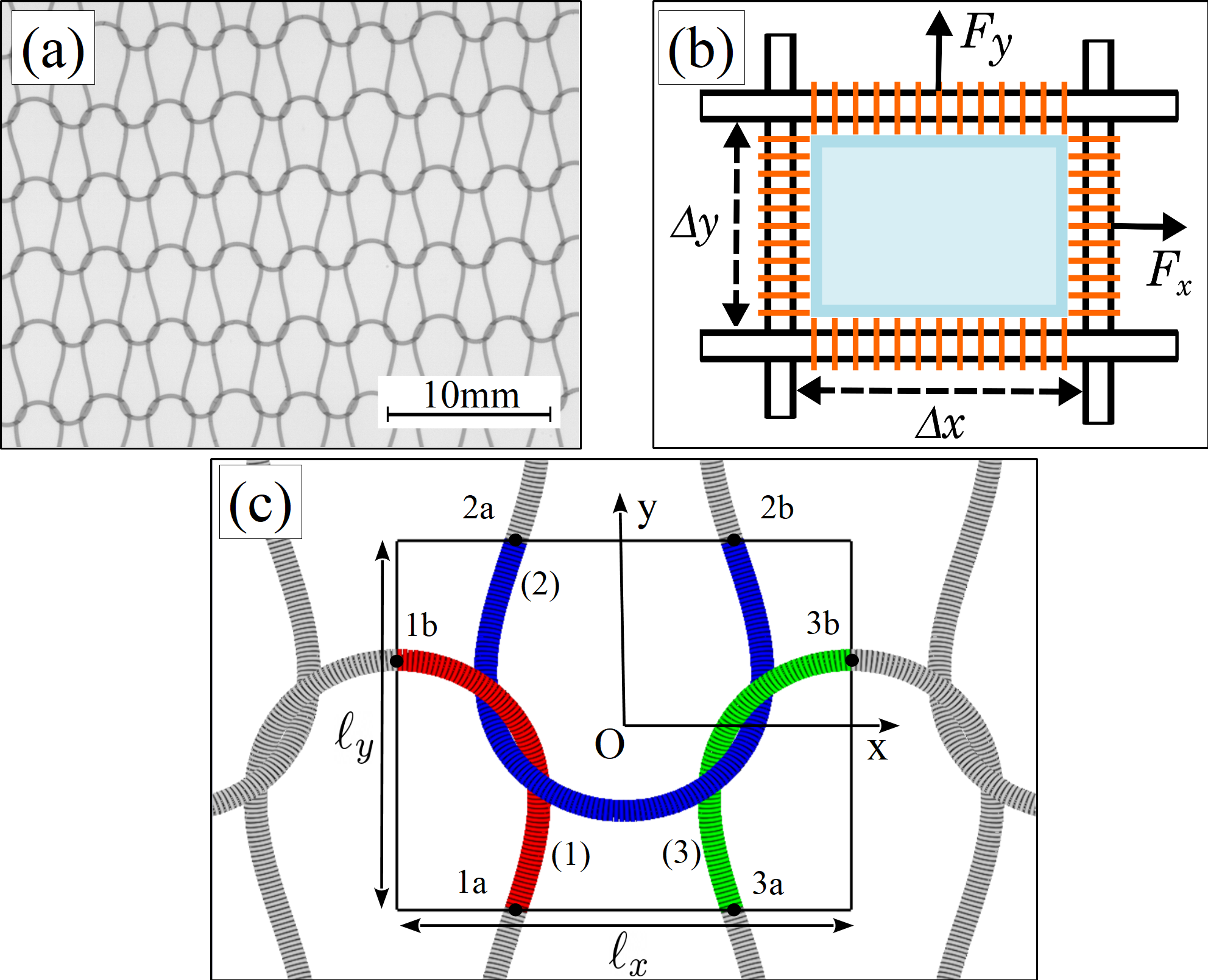
Figure 1: (a) Photo of a Jersey stitch knit. (b) Experimental set-up. The knitted fabric (light blue) is attached with metallic staples (orange) that can freely slide over 4 cylindrical bars linked to a biaxial tensile machine. (c) Geometry and numerical model. A rectangular cell of size $\ell_{x}\times\ell_{y}$ is composed of 3 threads $(1),(2)\&(3)$. Segments of cylinders composing the threads are colored. Dots $1a$, $1b$,… are the endpoints of the different threads, which are constrained to be on the cell boundaries with periodic boundary conditions.

In this study, we use a Jersey stitch knit, which is both simple and widely used. It consists of a single yarn forming interlocked loops as in fig. 1(a). Experimentally, we make a knitted fabric of $70\times 70$ stitches from a polyamide (Nylon) thread (Madeira Monofil n°40, $E=1.05~{}GPa$, $\mu=0.50$) of diameter $d=0.155~{}mm$. The length of thread per stitch is $\ell=9.7~{}mm$. The central $N\times N$ stitches ($N=50$) are attached to a biaxial tensile machine (fig. 1.b), where the spacing $\Delta x$ along the courses and $\Delta y$ along the wales can be varied by stepper motors. The forces per row $f_{x}\mathrel{\mathop{\mathchar 58\relax}}=F_{x}/N$ and columns $f_{y}\mathrel{\mathop{\mathchar 58\relax}}=F_{y}/N$ are measured using strain gauge force sensors. The network’s periodicity $(\ell_{x},\ell_{y})$ is obtained from images recorded with a camera. The network is also studied using numerical simulations based on Discrete Elastic Rods (DER) coupled with dry frictional contacts crassous_discrete_2023 . Threads are decomposed into segments of circular cylinders connected by springs, which account for the elastic forces of traction, flexion, and torsion. A mesh comprises 3 rods as shown in fig 1.c. The endpoints of these 3 wires are constrained to the $\pm\ell_{x}/2$ or $\pm\ell_{y}/2$ planes. Periodic boundary conditions in terms of positions and forces are applied at the junctions between the strands: for example, the strands $1$ and $2$ satisfy ${\bf r}_{2a}-{\bf r}_{1a}=\ell_{y}{\bf e}_{y}$, $\alpha_{2a}=\alpha_{1a}$, ${\bf r}^{{}^{\prime}}_{2a}={\bf r}^{{}^{\prime}}_{1a}$ and ${\bf r}^{{}^{\prime\prime}}_{2a}={\bf r}^{{}^{\prime\prime}}_{12}$. $\alpha$ is the torsion angle, ${}^{{}^{\prime}}$ and ${}^{{}^{\prime\prime}}$ are the 1st and 2nd derivatives with respect to the curvilinear abscissa $s$. Conditions on the derivatives ensure the continuity of the forces and moments.

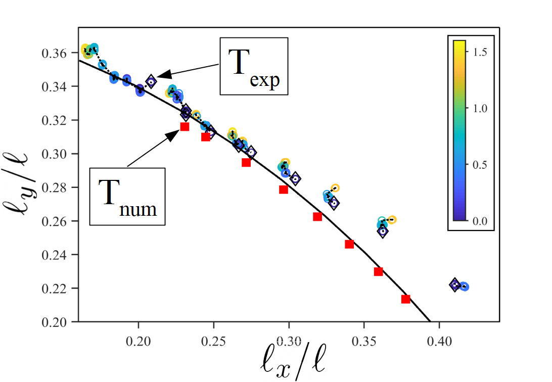
Figure 2: Relaxed configurations of a knitted fabrics ($\ell/d=62$, $\mu=0.5$). (open symbols): Experimental configurations during relaxation, color-coded by the value of $\log(f/f_{min})$. The dotted lines are guidelines. (black diamonds): Relaxed, experimental configurations; (red squares): Configurations obtained from DER simulations. There are no relaxed configurations above or to the left of the terminal points $T$, noted $T_{exp}$ (resp. $T_{num}$) for experimental (resp. numerical) data. (black plain line): Possible configurations expected from a 2D-elastica model with no applied stress.

The relaxed states are obtained as follows. Experimentally, the knitted fabric is stretched to an initial state $(\Delta x_{0},\Delta y_{0})$, then $\Delta x$ and $\Delta y$ are varied to reduce $f\mathrel{\mathop{\mathchar 58\relax}}=(f_{x}^{2}+f_{y}^{2})^{1/2}$ until it becomes lower than $f_{min}=8$ mN. Numerically, the knitted fabric is stretched, the forces are calculated. The stitch length is varied by $\delta\ell_{i}=-\lambda f_{i}$, with $i=x,y$ and $\lambda$ a numerical constant, until the force is smaller to a given threshold. Fig.2 shows the mesh sizes obtained following this experimental and numerical protocol. Firstly, the shape of the knitted fabric after the relaxation of the applied forces varies strongly with the initial state considered and is not uniquely defined. Secondly, these states are located on a curve which acts as an attractor in the space of $(\ell_{x},\ell_{y})$ configurations. This curve ends at a terminal point $T\mathrel{\mathop{\mathchar 58\relax}}=(\ell_{x_{T}},\ell_{y_{T}})$. A knit verifying $\ell_{y}>\ell_{y_{T}}$ or $\ell_{x}<\ell_{x_{T}}$ is impossible without external forces. Finally, the experimental and numerical data agreement is very satisfactory: assimilating a polyamide thread to an elastic fiber whose cross-sectional deformations are neglected is a reasonable hypothesis. The differences can be understood by noting that plastic deformations occur during knitting, meaning the stress-free yarn is no longer ideally rectilinear.

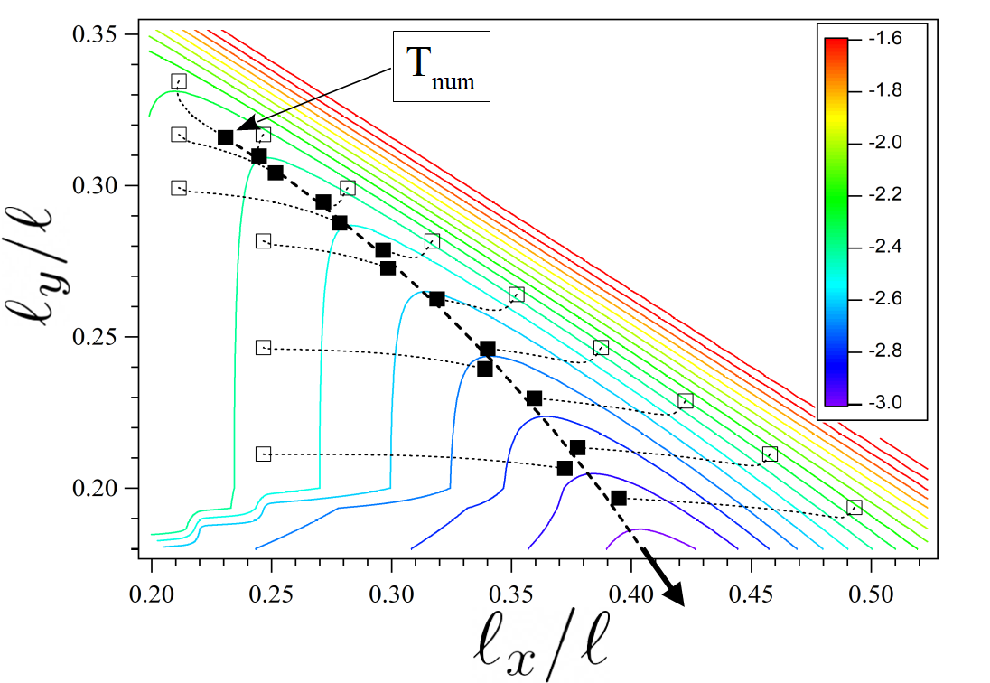
Figure 3: (Color): Curves of constant elastic energy $E$ for cells made of frictionless threads ($\mu=0$, $l/d=62$), color-coded by the values of $\log(E-0.01)$. (Dotted lines) Relaxation of fabrics with frictional thread ($\mu=0.5$) between an initial configuration (open square) and a relaxed configuration (filled square). $T_{num}$ is the terminal point. (Dashed curve): Relaxation of a fabric, initially at $T_{num}$, when $\mu$ is gradually decreased.

To describe the set of relaxed states, we first consider the elastic energy $E(\ell_{x},\ell_{y})$ of a frictionless knitted fabric. We obtain this quantity from DER simulation for each cell size at mechanical equilibrium. The iso-energy curves are shown fig.3. The traction zones (large $\ell_{x}$ or $\ell_{y}$) are separated from the compressive zones (small $\ell_{x}$ or $\ell_{y}$) by a valley that descends towards small $\ell_{y}$ and large $\ell_{x}$: the knitted fabric relaxes its bending energy by tending to align its yarns parallel to ${\bf e}_{x}$. The milder slope in this energy landscape acts as an attractor for knitted fabrics of finite friction. A knitted fabric initially placed on one side or the other of this line relaxes towards it and stops in its vicinity. Friction stops the deformation and allows metastability. The following numerical experiment can demonstrate this. We prepare a fabric with $\mu=0.5$ at its terminal point $T_{num}$. The friction coefficient is then decreased of $\delta\mu=-0.05$: the knitted fabric descends along the valley and stabilizes in a new position. By gradually reducing the friction, the line of milder slope (dashed line of fig.3) is followed toward the bottom of the valley. This line is the locus of terminal points obtained for different $\mu$.

Therefore, describing the set of metastable configurations requires i)understanding the shape of the valley, which a priori is independent of friction, and ii)knowing how the friction $\mu$ controls the position of the terminal point $T$ on the line of milder slope.

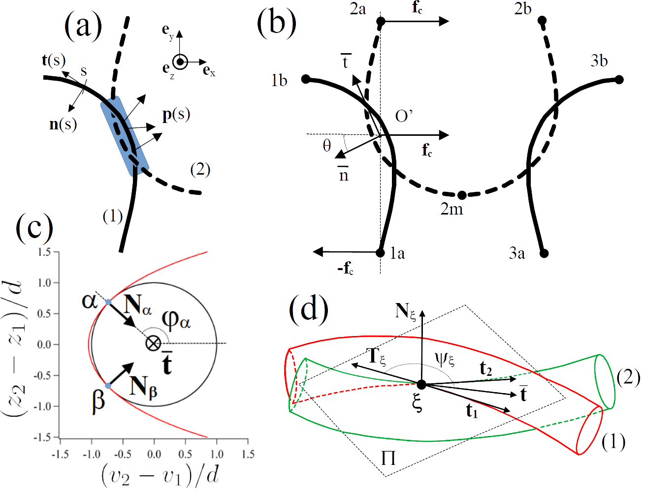
Figure 4: (a) Contact forces ${\bf p}(s)$ acting in the braid zone (blue rectangle) between two fibers. (b) Equilibrium of forces on the thread (1). The points $(1a)$ and $(2a)$ are on the vertical line of middle point $O^{\prime}$, and ${\bf{\overline{t}}}$ is the braid direction. (c) (Red line): Projection of the vector ${\bf r}_{2}-{\bf r}_{1}$, joining the centerlines, on the planes perpendicular to ${\bf{\overline{t}}}$. $v$ is the coordinate along an axis of direction $-{\bf{\overline{n}}}\mathrel{\mathop{\mathchar 58\relax}}={\bf{\overline{t}}}\times{\bf e}_{z}$. The circle is of unit radius. Contact occurs in two points $\alpha$ and $\beta$ (blue dots) that makes angles $\varphi_{\alpha}$ and $\varphi_{\beta}=-\varphi_{\alpha}$ with the $z=0$ plane. (d) Orientations of the contact force at a contact point $\xi$. The plane $\Pi$ containing ${\bf t}_{1}$ and ${\bf t}_{2}$ is normal to ${\bf N}_{\xi}$. ${\bf T}_{\xi}$ is the direction of the tangential contact force, which makes an angle $\Psi_{\xi}$ with ${\bf{\overline{t}}}$.

Interactions between the yarns take place in the area where they become entangled, creating both normal and tangential forces to the threads. This zone, schematically depicted in fig. 4.a, needs to be described. We introduce the curvilinear abscissa $s$ along the centerline of thread (1), and ${\bf p}(s)$ as the linear density of contact force exerted by (2) on (1). Because friction is present, ${\bf p}(s)$ is not necessarily aligned to the normal vector ${\bf n}(s)$. We define

$${\bf f}_{c}=\int_{s_{in}}^{s_{out}}{\bf p}(s)ds$$ (1)

the resultant of contact forces with $s_{in}$ the entrance of the contact zone: ${\bf p}(s_{in})\neq 0$ and ${\bf p}(s)=0$ for $s<s_{in}$, with reciprocal definition for $s_{out}$. For any relaxed state, we must have ${\bf f}_{c}\cdot{\bf e}_{y}=0$. Indeed (see fig.4.b), in the relaxed state, the total stress on each cell edge is $0$, so the external force on $(1b)$ is ${\bf f}_{1b}=0$. Since the force exerted by thread (2) on thread (1) is ${\bf f}_{c}$, we have ${\bf f}_{1a}=-{\bf f}_{c}$. No applied stress condition also implies ${\bf f}_{1a}+{\bf f}_{3a}=0$. Symmetry with respect to the $y$ axis at point (2m) implies ${\bf f}_{1a}\cdot{\bf e}_{y}={\bf f}_{3a}\cdot{\bf e}_{y}$, which leads to ${\bf f}_{c}\cdot{\bf e}_{y}=0$. It has been checked that the results of the simulations fulfilled all those requirements.

Let $s_{c}$ be the arbitrary abscissa at which ${\bf f}_{c}$ is applied. In the limit $d/\ell\ll 1$, we consider the bidimensional problem of finding the value of $f_{c}\mathrel{\mathop{\mathchar 58\relax}}=\|{\bf f}_{c}\|$ such that the 2D elastic curve ${\bf r}(s)$ representing the strand (1) is at equilibrium. The curve must satisfy the applied external force ${\bf f}_{c}$ at $s=s_{c}$ and $-{\bf f}_{c}$ at $s=s_{1a}=0$, and verifying $dy/ds=0$ at $s=s_{1b}=\ell/4$ and $\Bigl{(}{\bf r}(s_{c})+(d/2){\bf n}(s_{c})-{\bf r}(0)\Bigr{)}\cdot{\bf e}_{x}=0$. The last condition imposes contacts between the two threads in $O^{\prime}$. As shown on fig.4.c, the threads actually touch in two points but not in the middle point $O^{\prime}$. However, the distance between the centerlines in $O^{\prime}$ is typically $1.03~{}d\simeq d$. The solution of this 2D-elastica problem may be expressed with equations involving elliptic integrals. Since there is no explicit solutions, we solved this problem numerically. For each arbitrary value of $s_{c}$ we obtain $f_{c}$, ${\bf r}(s_{c})$ and ${\bf n}(s_{c})$. Using symmetries of the cell, we obtain:

$$\mathcal{L}_{x}(s_{c}) =\Bigl{(}4\bigl{[}{\bf r}(s_{c})-{\bf r}(\ell/4)\bigr{]}+2d~{}{\bf n}(s_{c})\Bigr{)}\cdot{\bf e}_{x}$$ (2a)

$$\mathcal{L}_{y}(s_{c}) =\Bigl{(}2\bigl{[}{\bf r}(s_{c})-{\bf r}(0)\bigr{]}+d~{}{\bf n}(s_{c})\Bigr{)}\cdot{\bf e}_{y}$$ (2b)

$(\mathcal{L}_{x}(s_{c}),\mathcal{L}_{x}(s_{c}))$ is the parametric curve in the plane $(\ell_{x},\ell_{y})$ shown on fig.2. This simple 2D approximation adequately captures the set of metastable points obtained from experiments and DER simulations.

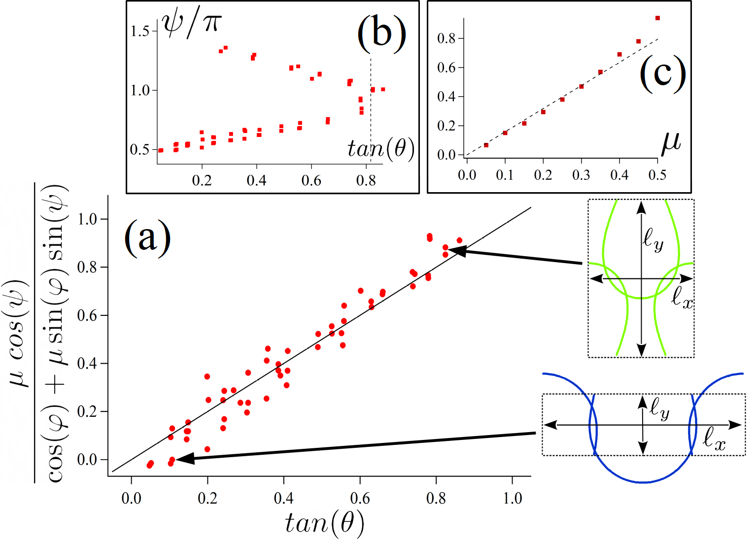
Figure 5: (a): $\mu~{}cos(\psi)/\bigl{[}\cos(\varphi)+\mu\sin(\varphi)\sin(\psi)\bigr{]}$ vs $\tan\theta$. Symbols are DER simulation results, and line is eq.(6). Insets are the threads centerlines for $\tan(\theta)\simeq 0$, and $\tan(\theta)\simeq\tan(\theta_{M})$. The dashed rectangles are the meshes of sizes $\ell_{x}\times\ell_{y}$. (b): Evolution of $\psi$ with $\tan(\theta)$. The maximal inclination $\tan(\theta_{M})$ (dashed line) is obtained for $\psi\simeq\pi$. Data of (a) and (b) are obtained for $\mu=0.5$. (c): Variation of $\tan(\theta_{M})$ with $\mu$. Dotted line is eq.(7) with $\varphi=129~{}deg$

All relaxed configurations $(\mathcal{L}_{x}(s_{c}),\mathcal{L}_{y}(s_{c}))$ are obtained using the condition ${\bf f}_{c}=f_{c}{\bf e}_{x}$ necessary to cancel the applied stress on one cell. We now discuss to which condition this constraint may be fulfilled. We consider the details of the contact force distribution ${\bf p}(s)$. The braid comprises two twisted fibers in a geometry similar to the one occurring in knots where the threads are twisted of $n$ turns. The cases $n=1$ ($3_{1}$ knot) audoly_2007 ; clauvelin_2009 , $n=2$ ($5_{1}$ knot) clauvelin_2009 and $n\gg 1$ jawed_2015 have been considered previously. Threads in the braid are approximately a helix contacting in a few points. It seems that our braid with $n=1/2$ has not been previously considered, but it exhibits a very similar behavior. The threads have nearly helical shape twisted around a common line of direction ${\bf{\overline{t}}}=\bigl{[}{\bf t}_{1}(s_{1})+{\bf t}_{2}(s_{2})\bigr{]}/\|{\bf t}_{1}(s_{1})+{\bf t}_{2}(s_{2})\|$, where ${\bf t}_{1}$ and ${\bf t}_{2}$ are the tangent vectors of centerlines of threads (1) and (2). The figure 4.c represents the relative position ${\bf r}_{2}(s_{2})-{\bf r}_{1}(s_{1})$ of the threads, where ${\bf r}_{1}(s_{1})$ and ${\bf r}_{2}(s_{2})$ are the projections of the centerlines on the plane perpendicular to ${\bf{\overline{t}}}$. The fibers are in contacts in two points $\alpha$ and $\beta$, and then:

$${\bf f}_{c}=\int{\bf p}(s)ds=\sum_{\xi=\alpha,\beta}\bigl{[}f_{\xi}^{(n)}{\bf N}_{\xi}+f_{\xi}^{(t)}{\bf T}_{\xi}\bigr{]}$$ (3)

with ${\bf N}_{\xi}$ the normal vector to the contact point, ${\bf T}_{\xi}$ the orientation of the tangential contact forces (see fig.4(d)), and $f_{\xi}^{(n)}$ and $f_{\xi}^{(t)}$ the normal and tangential forces. For all equilibrium configurations, we found $f_{\alpha}^{(n)}=f_{\beta}^{(n)}\mathrel{\mathop{\mathchar 58\relax}}=f^{(n)}$ and $({\bf N}_{\alpha}+{\bf N}_{\beta})\cdot{\bf e}_{z}=0$. Noting $\varphi_{\xi}$ the angle between ${\bf N}_{\xi}$ and $z=0$ (see fig.4.c), we have $\varphi_{\alpha}=-\varphi_{\beta}\mathrel{\mathop{\mathchar 58\relax}}=\varphi$, with $\varphi\simeq 3\pi/4$ for each relaxed configuration.

When the meshes are steadily deformed, the threads in contact make the braid slide. The friction is then fully mobilized, and $f_{\xi}^{(t)}=\mu f_{\xi}^{(n)}$. Since ${\bf N}_{\xi}\cdot{\bf t}_{i}(s_{\xi})=0$ for the two threads $i=1,2$, ${\bf N}_{\xi}$ is perpendicular to the plane containing ${\bf t}_{1}(s_{\xi})$ and ${\bf t}_{2}(s_{\xi})$. ${\bf T}_{\xi}$ belongs to this plane, and we may write:

$${\bf T}_{\xi}=\cos(\psi_{\xi})~{}{\bf{\overline{t}}}+\sin(\psi_{\xi})~{}\bigl{[}{\bf{\overline{t}}}\times{\bf N}_{\xi}\bigr{]}$$ (4)

where $\psi_{\xi}$ is the angle between ${\bf T}_{\xi}$ and ${\bf{\overline{t}}}$ (see fig.4.d). Using eq.(3) and eq.(4), we may calculate ${\bf f}_{c}$. With $\varphi_{\alpha}=-\varphi_{\beta}$, the equilibrium conditions ${\bf f}_{c}\cdot{\bf e}_{z}=0$ leads to $\psi_{\alpha}=-\psi_{\beta}\mathrel{\mathop{\mathchar 58\relax}}=\psi$, and finally:

$${\bf f}_{c}=2f^{(n)}\times\Bigl{(}\mu\cos(\psi){\bf{\overline{t}}}+\bigl{[}\cos(\varphi)+\mu\sin(\varphi)\sin(\psi)\bigr{]}{\bf{\overline{n}}}\Bigr{)}$$ (5)

The condition of mechanical equilibrium of a relaxed configuration ${\bf f}_{c}\cdot{\bf e}_{y}=0$ may then be written as:

$$\tan(\theta)=\frac{\mu~{}cos(\psi)}{\cos(\varphi)+\mu\sin(\varphi)\sin(\psi)}$$ (6)

In this equation, $\theta=\arccos({\bf{\overline{t}}}\cdot{\bf e}_{y})$ is the angle between the braid and y-axis. Fig.5.a shows the variations in the right and left members of eq.(6) for a fixed coefficient of friction $\mu=0.5$. The values of $\theta$, $\psi$, and $\varphi$ are measured at the various stopping points in fig.3, and the relationship eq.(6) is checked. The different $\theta$ values correspond to different aspect ratios of the meshes. For examples, insets of fig.5 shows configuration elongated in $x$ for $\theta\simeq 0$ and a configuration close to the terminal point $T$ for $\theta\simeq 40~{}deg$.

Given the expression of eq.(6), at a given friction coefficient, and $\varphi$ being roughly constant for all configurations, the only way to vary $\theta$ is to vary $\psi$, as can be seen clearly in fig.5.b. The tangential forces at the two contact points $\alpha$ and $\beta$ rotate on either side of the braid axis ${\bf{\overline{t}}}$. The effect of those rotations is to vary the amplitude of the total friction force along the ${\bf{\overline{t}}}$ axis, even if individual friction forces always evolve at the Coulomb threshold. Another consequence of eq.(6) is that $\tan(\theta)$ has a maximum value. With $\varphi\simeq 3\pi/4$ constant, $\tan(\theta)$ is maximal for a rotation $\psi=\pi-\arcsin(\mu)\simeq\pi$ for $\mu\ll 1$ (note that $\cos(\varphi)$ and $\cos(\psi)$ are negative), as shown in fig.5.b. This maximal value of $\theta$ is obtained when the frictional forces are roughly aligned with the common tangent of the centerline. Approximating $\psi=\pi$ in eq.(6), we finally obtain for small $\mu$:

$$\tan\theta\leq\tan(\theta_{M})\mathrel{\mathop{\mathchar 58\relax}}=\frac{\mu}{|\cos(\varphi)|}$$ (7)

where $\theta_{M}$ is the maximal value of $\theta$. This relation may be checked by measuring $\tan(\theta_{M})$ for different values of $\mu$. Fig.5.c shows that $\tan(\theta_{M})$ indeed follows eq.(7) with a constant $\varphi=129~{}deg$. For a given $\mu$, the maximal value of $\ell_{y}$ and minimal value of $\ell_{x}$ (corresponding to the terminal point $T$ of fig.2 and fig.3) is attained for $\theta=\theta_{M}$. When $\mu$ is varied, the line of terminal points (dashed line of fig.3) is traveled. On this line, $\theta=\theta_{M}(\mu)$, and $\psi\simeq\pi$, whatever is $\mu$: the friction forces are aligned and opposite to the relative displacements of the threads.

Our study rationalizes the relaxed states of a periodic yarn assembly. The relaxed state is not unique, but forms a continuous subset of the space of possible periodic configurations $(\ell_{x},\ell_{y})$ of a knitted fabrics. A terminal point (named T) bounds this subset. Those findings have many implications. Applying successive stretching cycles along $y$, the stitch size will converge to the terminal point $T$. The configuration corresponding to T would be the reproducible shape of a relaxed knitted fabric, even if metastability make other relaxed shapes possible. The existence of a continuum of relaxed states has important consequences for the macroscopic mechanical properties. The restoring forces are, therefore, weak over a wide range of the configuration space. Knitted fabrics are soft objects for deformations that remain in this zone but are relatively rigid when we move away from it. Finally, variations in aspect ratios mean that the area per stitch $\ell_{x}\times\ell_{y}$ can be varied at zero external force. A flat knitted fabric can thus be stretched to cover a surface with non-zero Gaussian curvature without any external forces being applied. This study can also serve as a ground basis for exploring further the mechanics of knitted fabrics or, more generally, of periodic structures made of threads with out-of-plane deformations or three-dimensional greer_2023 . The numerical and theoretical models can be adapted to different knitting topology singal_programming_2024 , but also for fibers closer to applications by modifying the elastic properties of the rod or smaller aspect ratio $l/d$. The methods introduced here are not limited to relaxed states but can also be adapted to explore the role of friction in the force vs. strain responses of textiles, including hysteresis poincloux.2018b and slip-induced fluctuations poincloux.2018 .

- (1) Paul Johanns, Changyeob Baek, Paul Grandgeorge, Samia Guerid, Shawn A Chester, and Pedro M Reis. The strength of surgical knots involves a critical interplay between friction and elastoplasticity. Sci. Adv., 9(23):eadg8861, 2023.
- (2) Christopher A Daily-Diamond, Christine E Gregg, and Oliver M O’Reilly. The roles of impact and inertia in the failure of a shoelace knot. Proc. R. Soc. A, 473(2200):20160770, 2017.
- (3) Nicholas Weiner, Yashraj Bhosale, Mattia Gazzola, and Hunter King. Mechanics of randomly packed filaments—the “bird nest” as meta-material. J. Appl. Phys., 127(5), 2020.
- (4) Gautier Verhille, Sébastien Moulinet, Nicolas Vandenberghe, Mokhtar Adda-Bedia, and Patrice Le Gal. Structure and mechanics of aegagropilae fiber network. Proc. Natl. Acad. Sci. U.S.A., 114(18):4607–4612, 2017.
- (5) Wilhelm Albrecht, Hilmar Fuchs, and Walter Kittelmann. Nonwoven fabrics: raw materials, manufacture, applications, characteristics, testing processes. John Wiley & Sons, 2006.
- (6) Caroline Vibert, Anne-Laurence Dupont, Justin Dirrenberger, Raphaël Passas, Denise Ricard, and Bruno Fayolle. Relationship between chemical and mechanical degradation of aged paper: fibre versus fibre–fibre bonds. Cellulose, pages 1–19, 2024.
- (7) Samuel Poincloux, Tian Chen, Basile Audoly, and Pedro M. Reis. Bending response of a book with internal friction. Phys. Rev. Lett., 126:218004, May 2021.
- (8) Antoine Seguin and Jérôme Crassous. Twist-controlled force amplification and spinning tension transition in yarn. Phys. Rev. Lett., 128(7):078002, 2022.
- (9) Julien Chopin, Animesh Biswas, and Arshad Kudrolli. Energetics of twisted elastic filament pairs. Phys. Rev. E, 109:025003, Feb 2024.
- (10) Andrew Craig Long. Design and manufacture of textile composites. Elsevier, 2005.
- (11) Robert Koerner. Geotextiles: from design to applications. Woodhead Publishing, 2016.
- (12) Samuel Poincloux, Mokhtar Adda-Bedia, and Frédéric Lechenault. Geometry and elasticity of a knitted fabric. Phys. Rev. X, 8:021075, Jun 2018.
- (13) Krishma Singal, Michael S. Dimitriyev, Sarah E. Gonzalez, A. Patrick Cachine, Sam Quinn, and Elisabetta A. Matsumoto. Programming mechanics in knitted materials, stitch by stitch. Nat. Commun., 15(1):2622, March 2024.
- (14) Guorui Chen, Yongzhong Li, Michael Bick, and Jun Chen. Smart textiles for electricity generation. Chem. Rev., 120(8):3668–3720, 2020.
- (15) Vanessa Sanchez, Conor J. Walsh, and Robert J. Wood. Textile Technology for Soft Robotic and Autonomous Garments. Adv. Funct. Mater., 31(6):2008278, February 2021.
- (16) D. L. Munden. THE GEOMETRY AND DIMENSIONAL PROPERTIES OF PLAIN-KNIT FABRICS. Journal of the Textile Institute Transactions, 50(7):T448–T471, July 1959.
- (17) Gamini Lanarolle. Geometry of compact plain knitted structures. Res. J. Text. Appar., 25(4):330–345, November 2021.
- (18) S. Allan Heap, Peter F. Greenwood, Robert D. Leah, James T. Eaton, Jill C. Stevens, and Pauline Keher. Prediction of Finished Weight and Shrinkage of Cotton Knits— The Starfish Project: Part I: Introduction and General Overview. Text. Res. J., 53(2):109–119, February 1983.
- (19) Jonathan M. Kaldor, Doug L. James, and Steve Marschner. Simulating knitted cloth at the yarn level. ACM Trans. Graph., 27(3):1–9, August 2008.
- (20) Georg Sperl, Rosa M. Sánchez-Banderas, Manwen Li, Chris Wojtan, and Miguel A. Otaduy. Estimation of yarn-level simulation models for production fabrics. ACM Trans. Graph., 41(4):1–15, July 2022.
- (21) Xiaoxiao Ding, Vanessa Sanchez, Katia Bertoldi, and Chris H. Rycroft. Unravelling the Mechanics of Knitted Fabrics Through Hierarchical Geometric Representation, July 2023. arXiv:2307.12360 [cond-mat].
- (22) Gabriel Cirio, Jorge Lopez-Moreno, and Miguel A. Otaduy. Yarn-Level Cloth Simulation with Sliding Persistent Contacts. IEEE Trans. Vis. Comput. Graph., 23(2):1152–1162, February 2017.
- (23) Jie Li, Gilles Daviet, Rahul Narain, Florence Bertails-Descoubes, Matthew Overby, George E Brown, and Laurence Boissieux. An implicit frictional contact solver for adaptive cloth simulation. ACM Trans. Graph., 37(4):1–15, 2018.
- (24) Dani Liu, Bahareh Shakibajahromi, Genevieve Dion, David Breen, and Antonios Kontsos. A Computational Approach to Model Interfacial Effects on the Mechanical Behavior of Knitted Textiles. J. Appl. Mech., 85(4):041007, April 2018.
- (25) Jérôme Crassous. Discrete-element-method model for frictional fibers. Phys. Rev. E., 107(2):025003, 2023.
- (26) Tomohiko G Sano, Emile Hohnadel, Toshiyuki Kawata, Thibaut Métivet, and Florence Bertails-Descoubes. Randomly stacked open cylindrical shells as functional mechanical energy absorber. Commun. Mater., 4(1):59, 2023.
- (27) B. Audoly, N. Clauvelin, and S. Neukirch. Elastic knots. Phys. Rev. Lett., 99:164301, Oct 2007.
- (28) N. Clauvelin, B. Audoly, and S. Neukirch. Matched asymptotic expansions for twisted elastic knots: A self-contact problem with non-trivial contact topology. J. Mech. Phys. Solids, 57(9):1623–1656, 2009.
- (29) M. K. Jawed, P. Dieleman, B. Audoly, and P. M. Reis. Untangling the mechanics and topology in the frictional response of long overhand elastic knots. Phys. Rev. Lett., 115:118302, Sep 2015.
- (30) Widianto P. Moestopo, Sammy Shaker, Weiting Deng, and Julia R. Greer. Knots are not for naught: Design, properties, and topology of hierarchical intertwined microarchitected materials. Sci. Adv., 9(10):eade6725, 2023.
- (31) Samuel Poincloux, Mokhtar Adda-Bedia, and Frédéric Lechenault. Crackling dynamics in the mechanical response of knitted fabrics. Phys. Rev. Lett., 121:058002, Jul 2018.