M-dwarf flares in the Zwicky Transient Facility data and what we can learn from them

Abstract

Aims. In this paper, we explore the possibility of detecting M-dwarf flares using data from the Zwicky Transient Facility data releases (ZTF DRs).

Methods. We employ two different approaches: the traditional method of parametric fit search and a machine learning algorithm originally developed for anomaly detection. We analyzed over 35 million ZTF light curves and visually scrutinized 1168 candidates suggested by the algorithms to filter out artifacts, occultations of a star by an asteroid, and known variable objects of other types.

Results. Our final sample comprises 134 flares with amplitude ranging from 0.2 to 4.6 magnitudes, including repeated flares and complex flares with multiple components. Using Pan-STARRS DR2 colors, we also assigned a corresponding spectral subclass to each object in the sample. For 13 flares with well-sampled light curves, we estimated the bolometric energy.

Conclusions. Our results show that the ZTF’s cadence strategy is suitable for identifying M-dwarf flares and other fast transients, allowing for the extraction of significant astrophysical information from their light curves.

1 Introduction

M-dwarf stars make up the vast majority of stars in our galaxy. As low-mass, fully convective stars, they exhibit frequent flaring events caused by powerful magnetic reconnection processes in their atmospheres (Gershberg & Pikel’Ner, 1972). The study of M-dwarf flares provides key insight into stellar magnetism, high-energy phenomena, and the impacts on potential planets orbiting these stars. However, many fundamental properties of M-dwarf flares remain poorly constrained, including their occurrence rates, energetics, and relationships with stellar properties such as age and metallicity (see for a review Kowalski 2024).

Multiple time-domain optical surveys have been utilised for systematic M-dwarf flare search projects. Space-based missions such as Kepler (Borucki et al., 2010) and TESS (Ricker et al., 2014) offer high regular cadence and very precise relative photometry, making their data excellent sources of stellar flares, especially those of small amplitude. Yang & Liu (2019) discovered approximately $1.6\times 10^{5}$ flares on around 3400 stars in the Kepler data. Günther et al. (2020) found 8695 flares in the first TESS data release, while Pietras et al. (2022) refined this number to roughly $1.4\times 10^{5}$ flares over three years of TESS data. While these space missions have revealed a vast number of stellar flares with good completeness, ground-based surveys could complement them. For instance, the Zwicky Transient Facility (ZTF; Bellm et al. 2019) covers sky areas that Kepler did not observe, with a bigger survey depth than TESS.

The recent advent of wide-field time-domain surveys provides new opportunities to build large statistical samples of stellar flares across a range of spectral types. Numerous systematic stellar-flare searches were performed with different ground-based surveys, occasionally observing high-amplitude flares. For example, Davenport et al. (2012) analyses hundreds of flares from SDSS and 2MASS time-domain surveys with the maximum $u$-band amplitude $\sim 4.5$ mag. The ASAS-SN M-dwarf flare catalogue counts 62 flares with the maximum amplitude being $\sim 2$ mag in the $V$-band (Rodríguez Martínez et al., 2020a). Webb et al. (2021) found 96 flares from 80 stars in the DECam data, with a maximum amplitude of $\sim 1.8$ mag. Aizawa et al. (2022) reveals 22 fast stellar flares from a one-second-cadence survey with Tomo-e Gozen with the largest amplitude of $\sim 3.25$ mag. Liu et al. (2023) presents a catalogue of 132 flares from 125 stars with amplitude up to $\sim 3.1$ mag found in two-year data of the Tsinghua University-Ma Huateng Telescopes for Survey.

In this work, we use photometric data from the Zwicky Transient Facility survey, which regularly monitors the northern sky from 2018 to detect transient events. ZTF runs multiple surveys, including a high-cadence survey, which provides a unique data set of minute-scale cadence with $\sim 21.5$ limiting magnitude (Kupfer et al., 2021). This makes ZTF data releases a source of well-sampled M-dwarf flare light curves occurring in a few hundred parsecs from the Sun. Crossland et al. (2023) used ZTF high-cadence survey for a systematic search for gravitational self-lensing binaries and presented 19 candidates. However, most of these candidates are likely to be stellar flares, making this data set to be the largest ZTF stellar flare catalogue previously published. Additionally, the SNAD team has discovered few stellar flares in ZTF data releases with our machine learning anomaly detection pipelines (Malanchev et al., 2020; Pruzhinskaya et al., 2023; Volnova et al., 2023).

Traditionally, flares are searched for by characteristic light-curve features, such as sharp brightening and a duration of up to a few hours. However, the diversity of flare shapes and the data volumes of ongoing wide-field surveys encourage the community to use machine learning techniques. The current paper uses both methodologies, which leads to the detection of a heterogeneous set of flaring stars. Since not all the candidates selected with these methods are stellar flares, we also conduct the dedicated one-by-one analysis to filter out bogus detections and objects of a different astrophysical origin.

This paper provides a catalogue of 134 flaring stars that we detected. We give the astrophysical properties of stars, such as spectral class and interstellar reddening. We also analyse well-sampled light curves to provide the total energy, amplitude, and timescale of the flares.

Our paper is structured as follows. In Section 2, we give an overview of the data sources used. In Section 3, we describe two methods for searching for stellar-flare candidates. In Section 4, we provide a description of our methodology for selecting flaring stars from the candidates. In Section 5, we analyse the physical properties of the flares and corresponding stars. In Section 6, we discuss the difference between the methods we used, the flare morphology and alternative interpretations of observed flaring light curves. We conclude our results in Section 7. Appendix A presents our catalog of ZTF flaring stars. Appendix B contains light curve plots of found M-dwarf flares candidates.

2 Data

The Zwicky Transient Facility is a wide-field astronomical survey of the entire northern sky, conducted with the 48-inch Schmidt-type Samuel Oschin Telescope at Palomar Observatory (Bellm et al., 2019). During phase I (Feb 2018 – Sept 2020), ZTF performed a three-day cadence survey of the visible northern sky and one-day for the Galactic plane. During phase II (Oct 2020 – Sept 2023), 50% of the ZTF camera time is dedicated to a two-day cadence public survey in $g$ and $r$ bands. Data from the public survey are released on a bi-monthly schedule as data releases (DRs). In addition, Kupfer et al. 2021 conducted a dedicated high-cadence Galactic plane survey with a cadence of 40 seconds.

In this work, we analyze the private and public data from ZTF DR8 (March 17, 2018 – September 3, 2021) as target data sets for searching for red dwarf flares. We used only ”clear” (catflags = 0) $r$- and $g$-band observations. ZTF DRs provide unique objects in each passband and observational field, so our dataset may have multiple light curves associated with a single source. In order to conduct further astrophysical analysis of the candidates found, we used data from additional catalogs: riz magnitudes from Pan-STARRS DR2 (Chambers et al., 2016; Flewelling, 2018), geometric distances from Gaia EDR3 (Gaia Collaboration et al., 2016, 2021; Bailer-Jones et al., 2021) and interstellar extinction from “Bayestar19” (Green et al., 2019) and Schlafly & Finkbeiner 2011 extinction maps.

3 Methods

In this paper we use two distinct approaches of M-dwarf flare identification. The first method is based on parametric search of flaring light curves in high-cadence subsample of ZTF Data Release 8 (DR8). The second method is based on an active anomaly detection approach applied to the full light curves of the entire ZTF DR8. We describe both methods in detail below.

3.1 Parametric fit search

As part of the ZTF survey, several different observational campaigns are conducted, including high-cadence survey (Kupfer et al., 2021). Unfortunately, bulk-downloadable ZTF DRs do not maintain the connection between each individual observation and the specific campaign to which this observation belongs. For this reason, it was necessary to develop a method for extracting high-cadence data from an entire DR.

The aim was to chunk light curves to form a dataset of intra-day light curves having: 1) enough observations for further analysis, 2) high cadence, and 3) covering the time interval typical for flare duration. To achieve the first two conditions, we set the minimum number of observations to 5 and the maximum delay between two consecutive observations to 30 minutes. As for the minimum duration of these partial light curves, it was decided to produce two samples, one with minimum duration of 2 hours (long-duration sample) and another with 30 minutes (short-duration sample). Such an approach allows us to detect both, short and long flares.

Along with the imposed conditions to the cadence and duration, all light curves were filtered according to observed source variability. We considered an object variable if a test based on 1-dimensional reduced $\chi^{2}$ statistics rejects the hypothesis about its non-variability (Sokolovsky et al., 2017):

$$\text{reduced}\leavevmode\nobreak\ \chi^{2}\equiv\frac{1}{N-d}\sum_{i}\left(\frac{m_{i}-\bar{m}}{\delta_{i}}\right)^{2},$$ (1)

where $m_{i}$ is the observed magnitude and $\delta_{i}$ its observational error, $\bar{m}$ is the weighted mean magnitude, $N$ is the number of observations and $d$ the number of model parameters. The final dataset consists of light curves with a value of the reduced $\chi^{2}$ statistics greater than 11. The total number of intra-day $r$-band light curve chunks in a long-duration sample is 4 027 686, and in a short-duration one is 10 351 985.

The parametric search method is based on light-curve fitting with an analytical function and selecting well-fit objects. For this purpose we adopt a semi-phenomenological model of flux evolution, $f(t)$, from Mendoza et al. (2022):

$$f(t)=f^{*}+\frac{\sqrt{\pi}AC}{2}\times\big{(}F_{1}\,h(t,B,C,D_{1})+F_{2}\,h(t,B,C,D_{2})\big{)}\,,$$ (2)

$$h(t,B,C,D)=\exp{(\alpha CD)}\times\text{erfc}(\alpha)\,,$$ (3)

$$\alpha(t,C,D)=\frac{B-t}{C}+\frac{1}{2}CD,$$ (4)

where $f^{*}$ is stellar (quiescence) flux density, $t$ is time, $A$ is the normalizing factor, $B$ is the reference time, $C$ is the Gaussian heating timescale, $D_{1}$ is the inverse of the rapid cooling phase timescale, $D_{2}$ is the inverse of the slow cooling phase timescale, $F_{2}\equiv(1-F_{1})\cdot\exp{(\frac{C^{2}}{4}(D^{2}_{1}-D^{2}_{2}))}$, where $F_{1}$ and $F_{2}$ describes the relative importance of the exponential cooling terms, and $\mathrm{erfc}$ is the complimentary error function. Note that here $A$ equals the value used by Mendoza et al. (2022) multiplied by $\exp{(B^{2}/C^{2}-D_{1}^{2}C^{2}/4)}$. We also changed the form of the equation by introducing the dimensionless function $\alpha(t,C,D)$ for better readability and robustness of the fit.

A Python function for fitting a light curve was implemented within the light-curve feature extraction library (Malanchev, 2021). This function chooses the optimal values of parameters $A$, $B$, $C$, $D_{1}$, $D_{2}$, $F_{2}$ and $f^{*}$ using least-squares fits provided by iminuit (Dembinski & et al., 2020). For better performance of the least-squares fitting, we used best-fit coefficients from the Markov Chain Monte Carlo analysis, presented in Mendoza et al. (2022), as initial values. The mean value of the $3\sigma$-clipped flux is used as the initial value of stellar flux $f^{*}$. The fit quality is evaluated using reduced $\chi^{2}$ statistics (Eq. 1) with $d=7$.

The next filtering step was to distinguish flares with enough points in the flare from ones with only a few points. For this reason, we used the OtsuSplit feature of the light-curve package (Lavrukhina et al., 2023). This feature uses a magnitude threshold to distinguish faint and bright subsamples of a light curve based on maximization of interclass variance. To filter out candidates, we used $\texttt{lower-to-all}>0.25$ (ratio of the number of points in the bright subsample to the number of points in the faint one) obtained for each object based on the determined threshold. However, this method does not guarantee perfect separation of the “flaring” part of the light curve from the “plateau”, so some candidates with few-point flares are still present in the final sample. The total number of candidates obtained with this procedure was 308.

3.2 Machine learning method

Active anomaly detection represents a family of machine learning techniques which sequentially uses expert feedback to fine-tune an initially standard unsupervised algorithm to a particular definition of scientifically interesting anomaly. In the implementation used in this work, we employ the Active Anomaly Discovery (AAD) algorithm developed by Das et al. (2018) in the form used by Ishida et al. (2019).

The algorithm starts from a traditional isolation forest (IF, Liu et al., 2008). It is based on the hypothesis that more objects in under-dense regions of the parameter space (statistical anomalies) are more rapidly isolated from the bulk of the data than nominal ones. In the first step of AAD, a traditional IF is built and the object with the highest anomaly score is shown to a human expert, who is required to provide a binary answer (“YES”/“NO”) to the question: is this anomaly scientifically interesting to you? The expert makes decisions based on both light curve behavior and auxiliary data, such as original scientific images and catalog cross-matches, see Section 4 for the details. If the answer is YES, the algorithm will show the second object with the highest anomaly score and pose the same question. Alternatively, if the expert answers NO, the algorithm recalculates the weights corresponding to the decision path which lead to that anomaly score. This modification is applied to the entire forest, the scores are recalculated, and the new object with the highest anomaly score is shown to the expert. After a few iterations, this procedure results in a personalized model which has a lower probability to give high anomaly scores to objects which are not in the expert’s main interest (full mathematical description is provided in Das et al., 2018).

Since the algorithm can be adapted to the opinion of the expert, it can be used for a targeted search for objects of a given type (see  Pruzhinskaya et al. 2023). Therefore, in this analysis, a human expert considered only M-dwarf flare candidates as anomalies; all other objects proposed by the algorithm are rejected by the expert as nominals.

The minimum number of observations per light curve was selected to be 300. To avoid nonvariable objects, we selected the reduced $\chi 2>3$ (Eq. 1, $d=1$). This selection resulted in 21 469 857 light curves.

We run AAD on the obtained data set and visually inspect 860 objects. Among those, we responded “YES” to 35 objects.

4 Sample selection

Visual inspection by human experts was a part of the sample selection process for both methods: as a final check of the parametric fit outputs, and at each iteration step of the AAD algorithm. All candidates were inspected using the SNAD ZTF Viewer, a special web interface developed by the SNAD team to facilitate expert analysis (Malanchev et al., 2023). For each object, the Viewer displays its multi-colour light curves and enables easy access to the individual exposure images and to the Aladin Sky Atlas (Bonnarel et al., 2000; Boch & Fernique, 2014). Moreover, it provides cross-matches with various catalogues of stars and transients, including SIMBAD and VizieR databases (Wenger et al., 2000), AAVSO VSX (Watson et al., 2006), Pan-STARRS DR2 (Flewelling et al., 2020), Gaia DR3 (Gaia Collaboration et al., 2023), and ZTF alert brokers^,,.

When deciding whether an event belongs to a red dwarf flare, we applied the following criteria:

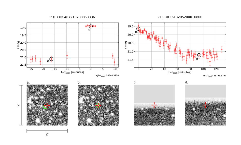
Figure 1: Light curves of a plateau (left) and an artefact (right) events discovered during the sample selection stage of flare identification. In the analysis of the light curve with a plateau in the peak, it was identified that such an increase in brightness is an overlap between the star and the asteroid 2003 XY 11. Two FITS images with different asteroid positions are presented at a. and b. subplots. The image scale is 1^′′ to 1 px. The right-hand panel shows a light curve that visually resembles a smooth decrease typical for red-dwarf flares, but analysis of its FITS files shows that its profile is due to the frame edge being on source localization. Two fits images with different frame edge position are presented at the c. and d. subplots.

• Light curve profile should be typical for a red dwarf flare: sharp increase in brightness followed by a smooth decrease. For example, the short-duration plateau observed during a “flare” is typically explained by the occultation of a star by an asteroid (left panel of Fig. 1).

• Absence of an artefact at the frame (satellite, edge of the frame, defocusing, ghost, bright star nearby, cosmics or hot pixels right panel of Fig. 1).

• The object should not be a known variable star, whose observed changes in brightness are caused by other processes.

Based on these criteria, we scrutinized 343 objects of both the parametric fit and the machine learning candidates. This resulted in a final dataset of 134 flaring M-dwarf stars. Only two flares (762109400005614,764114400003060) were found in ZTF $g$-band, the rest were identified in ZTF $r$-band. The remaining 209 candidates turned out to be artefacts (75 objects), instances of a star being occulted by an asteroid (128 objects) and parts of short-periodic star light-curves (6 objects).

The final sample of M-dwarf flares and their main characteristics are presented in Table LABEL:tab:Table_1. For M-dwarfs with recurrent flares, only the flare with the largest number of photometric measurements is listed. The first column contains the ZTF DR object identifiers (OIDs). The equatorial coordinates ($\alpha$, $\delta$) are presented in the second and third columns, respectively. The fourth column contains the geometric distance of each object estimated with Gaia EDR3 and its uncertainty (Bailer-Jones et al., 2021). In the fifth column, the object’s $A_{r}$ extinction is given (Schlafly & Finkbeiner, 2011; Green et al., 2019). The sixth, seventh, eighth, and ninth columns contain peak time, full width at half maximum (FWHM), amplitude, and number of points in the flare (see Sec. 5.2). The tenth column presents our spectral class prediction based on Pan-STARRS photometric colours. The last column contains notes. The next section provides detail of the analysis which led to columns four to nine.

5 Analysis

5.1 Flare energy

For further energy analysis, we used geometric distances derived from Gaia EDR3 (Bailer-Jones et al., 2021). Many candidates were found to be long-distant stars, for which distances have high uncertainties. We calculated the flare energy for the subsample of candidates whose Gaia DR3 parallax was measured with uncertainty not higher than 20%. We also keep candidates with enough points in the flare for higher quality of flare profile fitting. The final subsample consists of 13 flares that were used for the energy calculation.

We assume that flare radiation could be described by an optically thick black body with temperature $T_{\text{flare}}=9000$ K (Hawley & Fisher, 1992; Allred et al., 2006; Froning et al., 2019), so the bolometric luminosity, $L_{\textrm{f}lare}(t)$, is given by:

$$L_{\text{flare}}(t)=\rm{\sigma_{SB}}T^{4}_{\text{flare}}\mathcal{A}_{\text{flare}}(t)\,,$$ (5)

where $\rm{\sigma_{SB}}$ is the Stefan–Boltzmann constant, and $\mathcal{A}_{\text{flare}}(t)$ is the flare surface area that changes over time.

Now our objective is to estimate $\mathcal{A}_{\text{flare}}(t)$ from the observed flare flux. First, we introduce $\mathcal{A}_{\perp}$, a projection of $\mathcal{A}_{\text{flare}}$ in the picture plane. Then, the spectral flux density of the flare $F_{\nu}=\Omega B_{\nu}$, where $\Omega=\mathcal{A}_{\perp}/d^{2}$ is the solid angle of the flare as observed from distance $d$, and $B_{\nu}$ is the black-body intensity – Planck function.

We did not directly observe the spectral flux density with photometric surveys. Instead, its value was averaged over the passband transmission of the photometric filter in use. The averaged spectral flux density in ZTF $r$-band, $F_{r}$, is given by Koornneef et al. (1986):

$$F_{r}=\frac{\int F_{\nu}(\nu)/\nu\,R(\nu)\,\mathrm{d}\nu}{\int 1/\nu\,R(\nu)\,\mathrm{d}\nu}\leavevmode\nobreak\ =\leavevmode\nobreak\ \frac{\mathcal{A}_{\perp}}{d^{2}}\frac{\int B_{\nu}(\nu)/\nu\,R(\nu)\,\text{d}\nu}{\int 1/\nu\,R(\nu)\ \text{d}\nu},$$ (6)

where $R$ is the filter transmission function.

Using equation 6 we got $\mathcal{A}_{\perp}(t)$:

$$\mathcal{A}_{\perp}(t)=d^{2}\,\frac{F_{r}(t)}{B_{r}},$$ (7)

where $B_{r}$ is the black-body intensity averaged over $r$ passband. Being combined with Eq. (5) it gives the final expression of bolometric luminosity:

$$L_{\text{flare}}=\sigma_{\text{SB}}\,T^{4}_{\text{flare}}\,d^{2}\,\frac{\mathcal{A}_{\text{flare}}}{\mathcal{A}_{\perp}}\frac{F_{r}(t)}{B_{r}}\,.$$ (8)

Since we do not know the shape of the flare, we introduced the geometric factor $\mathcal{A}_{\text{flare}}/\mathcal{A}_{\perp}$. To be consistent with previous studies (Shibayama et al., 2013; Yang et al., 2017), we assume that this factor does not change with time and equals one.

Finally, we arrive at the expression for the bolometric energy:

$$E_{\text{flare}}=\int L_{\text{flare}}(t)\,\text{d}t\,.$$ (9)

This integral value depends only on the filter-averaged spectral flux density $F_{r}(t)$, which can be derived from observed magnitudes $m$. We convert observed magnitudes $m$ at time moments $t_{i}$ to fluxes taking into account extinction $A_{r}$ given by the 3-D map of Milky Way dust reddening (Green et al., 2019):

$$f(t_{i})=10^{-0.4(m(t_{i})-m_{0}-A_{r})}\,,$$ (10)

where $m_{0}$ is the AB-magnitude zero-point. To make the integral value more robust to observation uncertainties, we fit observations with the parametric function (2) and use these fitted model fluxes as a proxy to the filter-averaged spectral flux density: $F_{r}(t)=f(t)-f^{*}$.

The results of the energy calculations are given by Table 1.

oid	$E,10^{33}\,$erg
257209100009778	$88.95\pm^{15.44}_{11.26}$
283211100006940	$43.00\pm^{28.01}_{17.65}$
385209300066612	$6.71\pm^{2.70}_{1.54}$
412207100011243	$47.93\pm^{13.29}_{9.14}$
436207100033280	$13.15\pm^{3.13}_{2.36}$
437212300061643	$160.83\pm^{17.82}_{14.19}$
542214100014895	$7.74\pm^{0.32}_{0.32}$
592208400030991	$8.00\pm^{0.69}_{0.60}$
615214400005704	$404.08\pm^{195.02}_{87.72}$
726209400028833	$27.66\pm^{0.82}_{0.80}$
768211400063696	$7.21\pm^{2.10}_{2.00}$
771216100033044	$163.97\pm^{29.48}_{33.43}$
804211400018421	$36.34\pm^{20.74}_{9.54}$

Table 1: Bolometric energy estimations for the subsample of 13 flare candidates. The upper and lower bounds were defined according to the Gaia EDR3 estimated uncertainties on geometric distances.

5.2 Flare fit parameters

We used the same parametric function from (2) to estimate the amplitude, FWHM and number of points in the flare (Table LABEL:tab:Table_1). Firstly, a manual operation of flares’ observations subtraction from the full light curve was conducted – each stars’ light curve was trimmed to capture the flare itself and some amount of quiescent points which are necessary for the further fitting operation.

Secondly, for each flare, its profile was fitted using a parametric function (Equation (2)) to get a continuous representation convenient for further analysis. For complex light curves with several flare peaks, only the peak with the maximum amplitude (main peak) is considered for further fitting. The amplitude is calculated as the difference between the maximal and minimal model flux, which is achieved over a time interval. As a next step, the FWHM was measured as the difference between time points where the model curves possess values equal to half of the defined amplitude.

In order to define the number of points in the flare, we adopted the following criterion: all points of the light curve whose observed flux exceeds $f^{*}$ (quiescence stellar flux obtained from the model) by $3\sigma$, where $\sigma$ is the mean observational error of the selected part of the light curve, were considered as belonging to the flare.

5.3 Spectral class

Due to the lack of spectral information for most of our objects, we used a photometric approach to estimate their spectral types. We used stacked magnitudes from Pan-STARRS DR2 (Chambers et al., 2016; Flewelling, 2018) to build the ($r-i$, $i-z$) colour-colour diagram of our sample. The method in use is adopted from Kowalski et al. (2009) and allowed us to define the spectral subtypes of M-dwarfs based only on their photometric colours.

First, we corrected the colours for the galactic reddening. We used extinction values and coefficients from two different sources: the three-dimensional map of Milky Way dust reddening “Bayestar19” (Green et al., 2019), and, if this map does not contain the object, we used the map of Galactic Dust Reddening and Extinction presented by Schlafly & Finkbeiner 2011. Based on these maps, we calculated the final extinction value using:

$$\bm{A}=E\bm{R}$$ (11)

where $\bm{A}=(A_{r},A_{i},A_{z})$ represents the final extinction value in each filter, $\bm{R}=(R_{r},R_{i},R_{z})$ is the “extinction vector”, relating a scalar reddening to the extinction in each passband and $E$ is the reddening in the dust-map specific units. The extinction vector is $\bm{R}=(2.617,1.971,1.549)$ for the 3-D map “Bayestar19”, and $\bm{R}=(2.271,1.682,1.322)$ for the 2-D map of Galactic Dust Reddening and Extinction. For the 3-D map, we use Gaia EDR3 geometrical distance as discussed above.

Kowalski et al. (2009) proposed a table with the best-fit parameters of the two-dimensional Gaussian distribution for each M-dwarf spectral subtype in the ($r-i$, $i-z$) colour space. We calculated the probability of belonging to the corresponding spectral subclass following their proposal,

$$p_{m}(x)=\frac{1}{2\pi\|\Sigma_{m}\|^{1/2}}\exp(-\frac{1}{2}(\bm{x}-\bm{\mu}_{m})^{T}\Sigma_{m}^{-1}(\bm{x}-\bm{\mu}_{m}))\,,$$ (12)

where $m$ is an M-dwarf spectral subclass index, from 0 to 7, $\bm{\mu}_{m}$ and $\Sigma_{m}$ are Gaussian mean values and covariance matrix for this subclass, $\bm{x}=({r-i},{i-z})$ are deredded colors of the studied star.

For each star, we assigned the spectral subclass $m$ corresponding to the maximum probability $p_{m}$. We show the objects in the colour-colour diagram (Figure 2) with subclass corresponding to the point estimations of the pair of object’s colours. However, the deredded colour values may have large uncertainties associated with Pan-STARRS photometry error, distance estimation error (applicable only for the 3-D dust maps), and extinction errors.

Finally, we applied a colour cut based on West et al. (2008) and Bochanski et al. (2007), to construct a more pure M-dwarfs sample. Kowalski et al. (2009) presented the following limits, which take extinction into account: $(r-i)>0.42$, $(i-z)>0.23$.

From 134 stars found, we determined the spectral subclasses of $132$ of them (see Table LABEL:tab:Table_1, Figure 2). Five objects that lie outside of the M-dwarf limits might have a different spectral type. Their OIDs are 435211200068171, 540215200069194, 687207100049742, 687214100050598, and 768209200100383, with corresponding $A_{r}$ values of 1.14, 5.11, 1.15, 2.82, 2.67, respectively. It is possible that the interstellar reddening for these objects has been overestimated: four of them do not have Gaia distances, and for another, the distance is measured with high uncertainty, which may cause the object to appear shifted towards bluer colors.

For the 16 brightest objects, Gaia DR3 provides effective temperature estimations (Gaia Collaboration et al., 2023). We used these estimations to define a spectral class based on the relation between the stellar effective temperature and the spectral class for main-sequence stars adopted from Malkov et al. (2020). In all cases, this method confirms the spectral class M for these objects. For seven objects, we have an exact agreement for the spectral subclass between this method and the method based on Pan-STARRS colours. There is also an object (719206100008051) with available spectrum from SDSS DR18 (Almeida et al., 2023) data and the corresponding spectral classification, which is consistent with our colour-based classification. See the individual object information in the “note” column of Table LABEL:tab:Table_1.

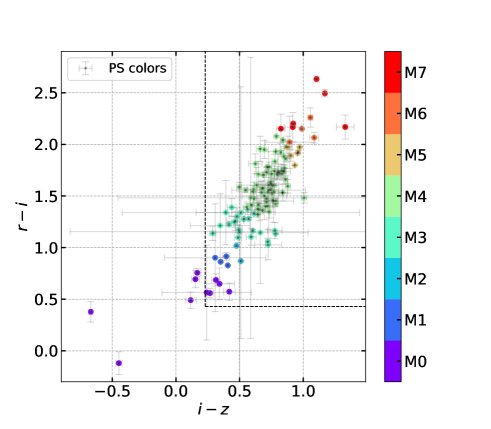
Figure 2: Spectral classes distribution calculated based on the photometric data from Pan-STARRS DR2. The black dashed lines show the blue limits of color indexes for the M-dwarf spectral type according to Kowalski et al. 2009. Five points that fall outside these limits likely belong to a different spectral class.

It should be noted that using Gaia geometric distances, we can estimate the absolute magnitude of our objects. The objects having much brighter absolute magnitude than expected for main-sequence M-dwarf stars (Pecaut & Mamajek, 2013), are found to have large parallax uncertainties. We mark the objects with large parallax uncertainties with crosses in the distance column of Table LABEL:tab:Table_1. Although most of the objects with more confident distance estimations are consistent with the main sequence, the outliers may be explained by system multiplicity or other systematic errors.

6 Discussion

6.1 Flares morphology

The flaring stars we study in this paper vary in the number of observational points per flare, flare recurrence, and light-curve profiles. The light curves of all the flares are provided in Appendix B.

For some of the flaring M-dwarfs multiple flares are observed: either multiple flares in a single passband (Fig. 3a), or a single flare simultaneously observed in $g$- and $r$-bands (Fig. 3b).

Additionally, we distinguish between classical and complex flare events on the basis of their temporal structure (e.g., Kowalski et al. 2013; Davenport et al. 2014). Classical flares have a single-peak profile, characterized by fast rise and exponential decay (Fig. 3c). However, the majority of our flares display a much more complex structure. This complexity ranges from relatively simple flares (see Fig. 3d) to highly complex flares consisting of multiple components (see Fig. 3e). According to Davenport (2015), studying such flare complexity could clarify their origins, as it remains uncertain whether they are produced by a single active region or by triggering separate nearby regions. In the first scenario, Davenport (2015) anticipates that the most energetic flare occurs first, followed by a sequence of less energetic events. However, this is not supported by some flares in our sample, where a less energetic peak precedes the most energetic one (Fig. 3f).

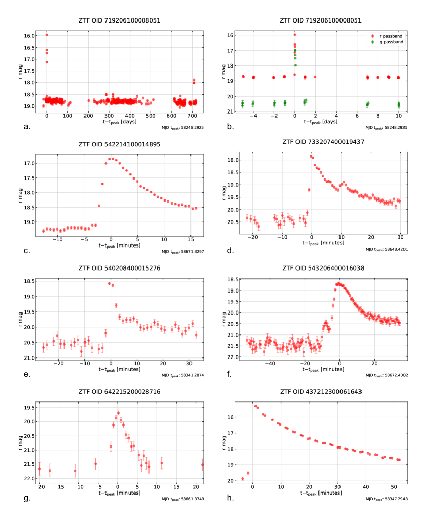
Figure 3: Light curves of M-dwarf flares with different morphology discovered with AAD (a-b, h) and parametric fit methods (c-g). a. Recurrent flares. b. Simultaneous flares in $g$- and $r$-bands. c. Classical singular flare with rapid rise and smooth decline. d. Complex flare with two components. e. Complex flare with multiple components. f. Complex flare with variable background, where a less energetic peak precedes the most energetic one. g. Flare with symmetric light-curve profile. h. Flare with highest magnitude amplitude.

Despite our best efforts, we recognize that there is still some inherited uncertainty in the classifications presented here, especially when only one point is available. They could be associated with hot spots on a stellar surface, self-lensing binaries or other types of stars that flare (e.g., Kowalski 2024). As it was recently stated by Crossland et al. 2023, a possible scenario would be self-lensing detached binaries, containing a stellar-mass neutron star or a black hole. The brightening occurs when the compact object transits the companion star. In that case, a symmetric light curve should be observed. Among our flares, there are a few candidates which satisfy this criteria (e.g., Fig. 3g).

6.2 Parametric fit vs AAD

Searching for flares on M-dwarfs is a complex task. Each set of data, whether it comes from different surveys or not, is unique. That is why it is so important to explore various searching strategies. In this paper, we applied two different methods for M-dwarf flares search. Below we compare both approaches.

First of all the parameters associated with the discovered flares are different. Due to the ZTF’s sporadic observation schedule, the flares found with AAD are sampled from incomplete light curves, often missing the peak brightness. In contrast, a parametric fit was applied to high-cadence data, thereby providing a well-defined light-curve profile of the flares. Consequently, flares found with AAD algorithm have systematically smaller amplitudes in comparison with the ones from the parametric fit (see Fig. 4(a)). The number of points in AAD flares is significantly lower, which makes them less reliable and harder to confirm. Also, recurrent flares were more often found by the AAD approach, since it had access to long-duration light curves (e.g., Fig. 3a).

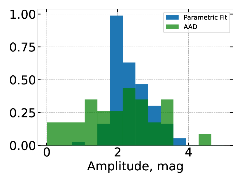
((a))

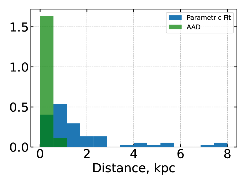
((b))

Figure 4: (a) Normalized histogram of amplitudes of flares found with parametric fit and AAD methods. (b) Normalized histogram of distances to M dwarfs found with parametric fit and AAD methods.

Secondly, regarding the spatial distribution of flares, the parametric fit search was limited by a ZTF high-cadence coordinate cut, resulting in flares that are located within the Milky Way plane. In contrast, the AAD does not have any coordinate restriction, yet the observed bias towards higher galactic latitudes in the Fig. 5 can be attributed to the selection effect, i. e. a fewer runs of the algorithm in fields within or close to the galactic plane, since this method requires expert evaluation at every step of its operation. Also, flares, obtained by parametric fit method, have a larger distance to Earth according to Gaia EDR3 (Fig. 4(b)). This can be explained by the use of a reduced $\chi^{2}$ metric to evaluate goodness of fit, which includes photometric errors, therefore lower metric quantities are systematically associated with fainter and more distant sources.

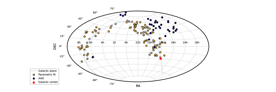
Figure 5: Spatial distribution of M dwarfs with flares in equatorial coordinates. Dark blue points indicate the flares found with AAD method, the yellow ones are flares detected with parametric fit search. Thin blue line shows the Galactic plane and red triangle is center of the Galaxy.

Finally, since AAD is an anomaly detection algorithm, it was not originally intended for flare detection. However, by treating flares as anomalies, we have been able to successfully adapt it to search for flares. It is interesting to note that only one over a few high-cadence flares identified by AAD exhibit exceptionally high amplitudes when compared to typical flare energy outputs (Fig. 3, see also Rodríguez Martínez et al. 2020b; Gorbachev & Shlyapnikov 2022). On the other hand, the parametric fit technique excels in isolating well-sampled flares within high-cadence amplitudes ZTF data, enabling the observation of complex substructures within the light curves (e.g, Fig. 3e). It allows performing a comprehensive analysis of individual flares (Davenport, 2015).

7 Conclusions

This paper is devoted to the search for M-dwarf flares in the eighth-data release of the Zwicky Transient Facility survey. We explored two different approaches: a parametric fit search and a machine learning method.

We visually scrutinized 1168 candidates, filtering out artefacts and known variables of other types, to identify 134 M-dwarf flares. This constitutes the largest sample of ZTF M-dwarf flares identified to date. The associations with the M spectral class was confirmed through the ($r-i$, $i-z$) colour diagram analysis, though some classifications may be incorrect, and we noted opportunities for identifying exotic events like self-lensing binaries. For 13 objects, we calculated the flare energy, ranging from $\sim$7$\times 10^{33}$ to $\sim$404$\times 10^{33}$ erg, which is consistent with the higher end of the energy distribution reported in the literature (Yang et al., 2017).

The comparison between the two approaches showed that each identifies flares of different parameters and distribution in the sky. For example, the parametric fit search found fainter flares, while AAD, despite lagging in flare light curve quality, identified recurrent flares. Additionally, the highest amplitude flare in the sample was discovered using AAD. Since each method has its own limitations, diverse strategies for flare detection are necessary to form a comprehensive picture of these phenomena.

Although the ZTF survey is not specifically designed for fast transients due to its 2-3 day cadence, it conducts private high-cadence observational campaigns. Such campaigns are also envisaged by the observational strategy of the Vera Rubin Observatory Legacy Survey of Space and Time. For the search and study of red dwarfs, we should not rely solely on dedicated surveys; instead, we must learn to extract necessary information from surveys not originally intended for this purpose. Therefore, developing methods for data filtering and flare identification are highly relevant.

In conclusion, ZTF data proved to be valuable for M-dwarf flare and other fast transient search, as well as being suitable for further astrophysical analysis.

Appendix A Table of M-dwarf flares

We show here the table of all found flares and the corresponding stars with their main characteristics.

ZTF DR OID	$\bm{\alpha}$, deg	$\bm{\delta}$, deg	distance, pc	$\bm{A_{r}}$, mag	$\bm{t}_{\mathrm{\bf peak}}$2, MJD$-$58000	FWHM2, hours	amplitude2, mag	n points2	spectral class	note
AAD method
257209100009778	92.9219	$-$22.7911	$195.41^{+16.28}_{-12.78}$	0.0000	471.3549	0.23444	3.01455	78	M7
437212300061643	287.9685	$-$1.9057	$171.94^{+9.28}_{-7.76}$	$0.0109^{+0.1871}_{-0.0109}$	347.2950	0.10187	4.55973	39	M4	Effective temperature available $2955.8^{+10.6}_{-19.6}$ K, M5
592208400030991	300.7593	17.5055	$130.01^{+5.46}_{-4.98}$	0.0000	343.2278	0.05552	3.54343	42	M7
634207400007102	255.6085	24.6610	$590.71^{+109.63}_{-89.24}$	0.1832	219.4415	–	3.45581	6	M4
676211100006667	218.9423	34.4342	$44.91^{+0.23}_{-0.19}$	0.0000	217.3884	–	0.90979	5	M3
677206300030165	228.0519	31.6719	$94.94^{+1.53}_{-1.60}$	0.0000	217.3703	–	3.09668	9	M6	Recurrent flares in $g$- and $r$- bands
678210100002177	237.5196	34.9555	$275.84^{+2.79}_{-3.29}$	0.1308	350.1435	–	0.61981	4	M3	Recurrent flares in $g$- and $r$- bands, effective temperature available $3408.1^{+3.7}_{-3.7}$ K, M2
718201300005383	212.5848	37.0767	$76.52^{+0.29}_{-0.26}$	0.0000	226.2941	–	0.98227	5	M4	Recurrent flares in $g$- and $r$- bands, simultaneous flares in both bands
719206100008051	219.6046	39.6384	$126.23^{+6.16}_{-4.84}$	0.0000	248.2924	–	2.60198	4	M5	Recurrent flares in $g$- and $r$- bands, simultaneous flares in both bands, spectrum available, SDSS J143825.07+393819.5, M5
719216300003437	213.9701	42.9291	$391.43^{+4.99}_{-4.74}$	0.0000	222.3259	–	0.22239	4	M2	Flares in $g$- and $r$- bands, effective temperature available $3592.5^{+11.1}_{-2.1}$ K, M1
721201200001366	238.6182	38.3407	$101.37^{+1.47}_{-1.50}$	0.0000	216.3633	–	2.09871	3	M5
726209400028833	282.5514	40.8524	$162.36^{+2.38}_{-2.37}$	0.0000	324.3501	0.12602	1.78179	65	M4	Effective temperature available $3231.9^{+5.5}_{-5.3}$ K, M3
756211200000623	192.6775	49.4891	$192.50^{+10.25}_{-9.49}$	0.0000	217.2386	–	2.34364	1	M4	Flares in $g$- and $r$- bands
761214100001680	245.8604	51.3084	$274.63^{+12.79}_{-10.89}$	0.0000	216.3775	–	2.76476	5	M4	Effective temperature available $3093.7^{+3.1}_{-1.9}$ K, M4
762109400005614	257.9108	47.7715	$126.54^{+0.46}_{-0.43}$	0.0000	635.4311	–	1.37889	4	M3
762201400007313	258.2507	44.1310	$150.43^{+2.80}_{-2.91}$	0.0000	377.1626	–	3.47028	3	M4	Recurrent flares in $r$-band, one simultaneous flare in both bands, effective temperature available $2966.4+^{9.7}_{-6.8}$ K, M5
764114400003060	275.3463	50.2501	$238.04^{+1.09}_{-1.22}$	0.0000	691.3068	–	0.27586	1	M1	Effective temperature available $3805.7^{+6.6}_{-4.5}$ K, M0
764203100012551	271.8373	44.9095	$480.39^{+46.77}_{-28.06}$	$0.1308_{-0.0205}$	198.5153	–	1.97728	3	M2	Effective temperature available $3249.5^{+35.6}_{-22.3}$ K, M3
791209200005999	205.9704	55.9733	$289.52^{+10.94}_{-13.54}$	0.0000	248.2657	–	1.46843	4	M4	Recurrent flares in $r$-band, effective temperature available $3210.1^{+8.7}_{-8.8}$ K, M4
792207200006505	211.3704	54.1319	$93.68^{+0.28}_{-0.34}$	0.0000	258.2268	–	1.52560	4	M4	Recurrent flares in $g$- and $r$- bands, one simultaneous flare in both bands, effective temperature available $3236.1^{+1.9}_{-4.0}$ K, M3
795213200016815	251.0949	57.8094	$153.76^{+2.51}_{-1.90}$	$0.0124^{+0.0074}_{-0.0057}$	262.3504	–	2.33200	2	M4	Recurrent flares in $g$- and $r$- bands, effective temperature available $3169.7^{+4.5}_{-3.9}$ K, M4
796214100003950	259.9339	58.2575	$33.87^{+0.03}_{-0.04}$	0.0000	379.2584	–	1.08040	1	M5	Recurrent flares in $g$- and $r$- bands, effective temperature available $2974.1^{+4.2}_{-7.6}$ K, M5
798207400001244	279.1108	53.9023	–	0.0899	318.3486	–	0.52966	4	M1	Recurrent flares in $g$- and $r$- bands, simultaneous flares in both bands
798209400009221	284.9472	55.2334	$264.90^{+18.62}_{-13.75}$	0.0000	198.5135	–	2.16658	3	M4	Flares in both $g$- and $r$- bands
821216100003336	200.1288	65.2912	$282.43^{+5.75}_{-5.59}$	0.0000	353.1419	–	1.39329	2	M4	Effective temperature available $3285.1^{+21.8}_{-7.5}$ K, M3
824205200007029	250.7534	61.4259	$397.62^{+60.71}_{-48.00}$	0.1570	377.1581	–	2.33040	1	M4
825213100013108	267.8115	64.9554	$186.73^{+10.76}_{-8.28}$	0.0000	325.2432	–	3.25031	4	M4
848205100005466	274.1424	68.5419	$91.45^{+0.41}_{-0.53}$	0.0000	385.1791	–	2.73741	3	M4	Recurrent flares in $g$-band and a flare in $r$-band
857207100012456	81.2459	76.2029	$242.02^{+3.42}_{-4.33}$	$0.2094_{-0.0429}$	358.4232	–	2.36735	3	M3	Effective temperature available $3364.6^{+4.4}_{-5.1}$ K, M3
858204400004738	100.5724	73.0318	$398.96^{+27.84}_{-18.38}$	0.2617	229.1904	–	1.82581	1	M2	Recurrent flares in $r$-band, effective temperature available $3491.1^{+12.5}_{-12.4}$ K, M2
858213100000788	126.4006	79.6325	$638.21^{+61.31}_{-53.07}$	0.1308	464.3079	–	1.19362	1	M3	Effective temperature available $3392.0^{+23.8}_{-25.3}$ K, M2
1866210400023756	78.2604	73.1147	$59.19^{+0.42}_{-0.43}$	0.0000	774.3110	–	2.54463	3	M7	Recurrent flares in $r$-band
Parametric fit method
257214400014856	91.0585	$-$22.0385	${}^{\dagger}1392.66^{+1373.00}_{-707.61}$	0.1308	468.3190	0.09414	1.62995	19	M4
260208100017563	109.4550	$-$24.6727	${}^{\dagger}1237.22^{+596.11}_{-397.29}$	$0.2355^{+0.0662}_{-0.0785}$	493.3462	0.04697	2.53987	32	M4
262201300031816	129.7493	$-$27.8083	–	0.2542	493.3885	0.15505	2.71971	33	M7
280214400089687	259.6615	$-$21.6633	${}^{\dagger}702.36^{+293.14}_{-188.09}$	$1.3500^{+0.1417}_{-0.1083}$	303.2693	0.04313	1.99418	30	M4
281201100016537	268.6979	$-$26.5830	${}^{\dagger}1223.03^{+1021.79}_{-669.60}$	$2.3154^{+0.2766}_{-1.9040}$	636.3873	0.24195	2.05648	36	M3
283211100006940	279.3314	$-$22.5463	$519.19^{+148.03}_{-120.53}$	$0.4972^{+0.0523}_{-0.0262}$	312.2717	0.04116	2.21516	9	M4
284212100096997	284.2108	$-$22.6351	${}^{\dagger}5038.87^{+2562.02}_{-2095.08}$	0.6804	287.3557	0.07169	2.31607	24	M4
308214300027206	100.8986	$-$14.8462	${}^{\dagger}707.18^{+331.81}_{-192.67}$	$0.3921^{+0.3930}_{-0.1304}$	464.3919	0.03514	2.55428	34	M4
309208200034266	104.3670	$-$17.7464	–	1.5852	464.3837	0.09362	2.47916	13	M0
310212300021722	111.9763	$-$16.8197	${}^{\dagger}1145.06^{+547.17}_{-419.21}$	$0.5234^{+0.5234}_{-0.0262}$	475.4510	0.05547	2.47399	37	M3
332213200128168	271.9229	$-$14.1020	${}^{\dagger}1548.68^{+2089.12}_{-852.08}$	$1.3555^{+2.3197}_{-0.2302}$	637.3692	0.29056	1.91586	123	M2
334203400074200	283.5040	$-$20.3306	${}^{\dagger}5221.32^{+2086.45}_{-2273.88}$	$0.8374_{-0.1832}$	320.3401	0.03386	2.87705	17	M4
336202400036948	299.2203	$-$20.7151	${}^{\dagger}375.64^{+109.16}_{-75.84}$	$0.4972_{-0.0766}$	667.4013	0.06337	2.46815	41	M4
336212400006103	295.0432	$-$16.2609	–	0.3741	667.3851	–	0.82742	16	M4
367206100004253	161.5502	$-$10.4167	$174.61^{+12.73}_{-10.62}$	0.0000	511.2607	0.04158	2.12943	18	M7
385209300066612	290.2818	$-$9.3424	$252.81^{+46.63}_{-30.98}$	$0.4304^{+0.0930}_{-0.2074}$	292.4055	0.04154	2.59133	21	M4
410210100030608	101.6796	$-$1.0568	–	2.3353	812.4599	0.06651	2.98777	33	M0
410215100032143	99.6352	0.5756	${}^{\dagger}1214.56^{+1149.74}_{-819.13}$	$0.5856^{+0.5397}_{-0.5594}$	812.4650	0.03854	2.17184	20	M4
410216400016069	97.7781	$-$0.3300	${}^{\dagger}2845.78^{+2208.58}_{-1154.52}$	$1.6008^{+0.4928}_{-0.3084}$	812.4972	0.08735	1.79725	24	M3
411203400031073	106.8275	$-$6.3215	${}^{\dagger}4538.29^{+3644.30}_{-2657.60}$	$1.2896^{+0.3330}_{-1.0279}$	457.3170	0.05976	2.39444	36	M4
412201100010804	117.6872	$-$5.1527	–	0.2787	456.4139	0.21868	2.23172	41	M2
412207100011243	114.1311	$-$3.1612	$248.12^{+32.29}_{-24.91}$	$0.0206^{+0.0056}_{-0.0206}$	456.5040	0.07497	3.12722	14	M5
412212400027889	112.2499	$-$1.9847	–	0.2395	457.4206	0.05865	3.82644	21	M4
413211400001358	121.0392	$-$1.7560	${}^{\dagger}1436.95^{+895.33}_{-590.04}$	0.0785	775.4796	0.10116	1.87288	65	M4
435211200068171	275.6615	$-$1.4027	–	2.5958	640.4373	–	1.80464	1	M0
436207100033280	283.7603	$-$3.3619	$376.80^{+42.50}_{-35.43}$	$0.7351^{+0.0500}_{-0.0285}$	347.3100	0.06881	2.18643	15	M4
436214200040092	284.6744	0.8566	${}^{\dagger}455.63^{+114.79}_{-79.21}$	$0.7328^{+0.2668}_{-0.1047}$	348.2973	0.09092	1.93071	40	M4
437203100058319	291.2111	$-$4.7123	${}^{\dagger}2765.85^{+1634.56}_{-1467.85}$	$1.4917^{+0.1570}_{-0.1570}$	348.3126	0.21199	1.91068	27	M4
437211400092016	291.2327	$-$1.8312	${}^{\dagger}3683.40^{+1707.96}_{-1886.50}$	$0.6804^{+0.1832}$	347.3185	0.17083	2.95975	19	M3
461216200033263	99.9443	7.4280	–	2.1996	853.2143	0.09151	1.84815	19	M3
462201300001148	112.7258	1.6316	${}^{\dagger}2524.95^{+1756.09}_{-1004.31}$	$0.3926_{-0.0188}$	482.4555	0.11739	2.28222	27	M3
486211400004409	274.1717	5.4338	${}^{\dagger}3099.40^{+1958.82}_{-1648.63}$	$0.5496_{-0.0804}$	643.4100	0.11097	1.78638	33	M4
487207400067044	280.5736	3.2671	${}^{\dagger}853.25^{+1527.94}_{-291.60}$	$2.1523^{+1.0928}_{-0.9774}$	644.4040	0.06409	1.73718	32	M2
488203200156038	286.7733	2.1147	${}^{\dagger}4936.48^{+2652.39}_{-2073.99}$	$3.1927^{+0.0262}_{-0.1570}$	340.2434	0.15744	2.07865	18	M0
491203400002897	308.7275	1.5507	–	0.1863	670.3563	0.10956	2.05567	24	M3
536204200026434	260.4943	8.9845	–	0.2463	634.3900	0.11730	1.65854	33	M4
537204100031453	268.7043	9.6602	–	0.5060	665.4077	0.06055	2.05396	24	M4
539209100126426	288.1225	12.9930	${}^{\dagger}2767.03^{+616.65}_{-513.43}$	$3.9255^{+0.1047}_{-0.0785}$	334.2062	0.07879	3.41830	19	M0	Present in DR8, absent in DR17
540208400015276	289.8905	10.4382	$321.89^{+49.02}_{-37.51}$	$0.6885^{+0.0383}_{-0.1889}$	341.2874	0.04033	2.16345	23	M6	Recurrent flares in $g$- and $r$- bands
540215200069194	290.4086	14.9622	–	11.6013	342.2201	–	3.03899	19	M0
542214100014895	307.2230	15.0669	$125.11^{+2.53}_{-2.64}$	0.0000	671.3297	0.08716	2.48119	29	M4
543206400016038	314.4593	10.0783	${}^{\dagger}1252.52^{+1561.89}_{-690.48}$	$0.2617_{-0.0523}$	672.4002	0.16202	2.76272	69	M4
543215400016323	312.3468	13.9935	–	0.2313	672.4067	0.07693	2.11956	19	M4
562216200020648	84.6147	22.3520	–	2.6877	852.2416	0.11486	2.33459	40	M1
563202400050273	96.8058	15.3731	${}^{\dagger}599.07^{+344.88}_{-187.01}$	$0.3218^{+0.3324}_{-0.2800}$	862.2359	–	2.31834	104	M3
565209300016509	112.6538	19.2998	–	0.0811	795.3952	0.10856	2.16999	41	M3
588211300040671	272.7993	19.6388	–	0.2051	645.4004	–	2.53612	6	M4
588212300042173	271.0911	19.3271	${}^{\dagger}5856.62^{+2846.60}_{-3822.58}$	0.4187	645.3718	–	1.86149	3	M2
592201300048015	306.0703	15.7461	–	0.4941	344.1939	–	2.71258	12	M3
611215200019569	82.1163	29.4668	–	1.5365	846.1697	0.07061	2.50922	33	M4
613214200021207	98.8276	29.4430	–	0.4955	791.4480	0.06009	1.65899	14	M4
615210400006263	115.5509	26.5841	–	0.0991	849.2762	0.15224	2.54879	8	M5
615214400005704	114.8512	28.5188	$496.64^{+108.08}_{-57.20}$	$0.0785^{+0.0262}_{-0.0262}$	846.3346	0.26036	2.62912	20	M4	Recurrent flares in $r$-band
616216400012099	118.0565	28.6515	–	0.0864	812.5463	–	3.06957	6	M5
642215200028716	314.0120	29.1802	–	0.3274	661.3749	0.05116	2.04285	10	M4
642215300060146	314.5377	28.5770	–	0.4228	802.1148	0.26050	1.79666	55	M3
655210200003936	55.9941	34.8996	${}^{\dagger}1044.42^{+669.57}_{-358.90}$	0.7851	789.3148	0.12400	3.80780	8	M4
660207200039946	92.7499	32.5936	–	1.3037	790.4454	0.15593	2.46155	44	M3
660207300043882	92.0245	32.0495	–	1.5532	790.4520	0.06394	2.17576	19	M4
660209300008318	97.2417	33.7800	–	0.6422	790.4604	0.18062	1.90401	26	M4
684209200042442	285.7614	35.1056	${}^{\dagger}2347.42^{+1476.64}_{-964.59}$	$0.2617^{+0.0262}$	299.2711	0.10895	1.92677	41	M4
685205100007414	294.3103	33.0739	${}^{\dagger}3403.98^{+1480.39}_{-1627.35}$	$0.3537^{+0.1986}_{-0.0658}$	345.2225	0.01509	3.42933	15	M4
685211100071699	289.4993	34.4177	–	0.3306	345.2271	0.14859	1.87430	17	M3
686201100023141	302.3502	30.7379	${}^{\dagger}4042.33^{+2290.52}_{-1536.73}$	$3.4090^{+0.1061}_{-0.4143}$	346.2240	0.27842	1.85088	26	M0
686208200055661	294.3102	33.0738	${}^{\dagger}3403.98^{+1480.39}_{-1627.35}$	$0.3537^{+0.1986}_{-0.0658}$	345.2221	0.10247	2.59321	18	M4
687207100049742	305.8142	33.1314	${}^{\dagger}2966.10^{+1774.93}_{-1357.79}$	$3.0095^{+0.1832}_{-0.5557}$	658.3663	0.04862	3.03718	36	M0	Recurrent flares in $r$-band
687214100050598	307.4067	36.2972	–	6.4051	658.3508	0.16569	2.56898	40	M0
688214300032111	313.9940	35.6929	${}^{\dagger}541.88^{+768.49}_{-142.82}$	$0.2187^{+0.4356}_{-0.1402}$	450.1517	0.04322	3.51725	13	–
689211400045274	320.7232	33.7768	${}^{\dagger}1836.04^{+1467.16}_{-721.42}$	$0.4187^{+0.0262}_{-0.1832}$	449.1489	0.18553	1.88723	21	M4
690210100033851	331.0012	34.3635	–	0.3364	660.3650	0.10866	3.21347	47	M4
700213100014818	58.7839	43.5987	–	1.0205	793.3194	0.08245	2.01478	17	M4
704203100027996	88.6826	37.8677	${}^{\dagger}5060.59^{+5223.01}_{-3068.89}$	$1.0206_{-0.1832}$	812.3948	0.05178	2.97422	43	M4
706208200005412	101.8098	39.9440	–	0.3238	793.3987	0.11954	2.19620	22	M2
728205100116115	299.7507	39.8352	${}^{\dagger}7906.58^{+4266.19}_{-2987.71}$	$0.8374_{-0.0785}$	437.0989	0.07523	1.92979	11	M2
733207400019437	337.1025	38.7816	${}^{\dagger}898.49^{+581.59}_{-194.95}$	$0.2094^{+0.0262}_{-0.0262}$	648.4201	0.05229	2.54306	49	M4
733209300032227	341.4235	40.9291	–	0.3876	648.4221	0.12216	2.26885	29	M4
742211400023238	61.8394	47.9758	–	2.8823	806.4472	0.06852	2.32372	21	M3
766203400032547	292.2349	44.4207	${}^{\dagger}422.97^{+156.86}_{-83.71}$	$0.0785^{+0.0262}_{-0.0785}$	295.4018	0.17767	1.50524	29	M4
766205100052523	297.4471	47.3023	${}^{\dagger}770.36^{+284.14}_{-203.85}$	$0.0785^{+0.1006}_{-0.0523}$	294.4330	0.14369	1.82875	22	M4
767206100019391	304.8313	47.2899	${}^{\dagger}4526.71^{+3963.91}_{-2037.80}$	$1.7534^{+0.0262}_{-0.4972}$	448.1220	0.14390	2.51425	19	M4
767212100038888	299.2655	49.0555	–	0.3939	448.1118	0.11812	1.94437	11	M4
768202400043820	313.9297	44.2798	$178.57^{+32.63}_{-25.55}$	0.0000	448.1355	0.05168	3.16981	10	M6
768209200100383	316.0178	49.1134	–	6.0695	451.1700	0.04848	2.93990	8	M0
768211400063696	311.4420	48.4437	$243.37^{+33.22}_{-36.45}$	$0.0236^{+0.1954}_{-0.0236}$	448.1217	0.07152	2.04332	18	M6
771211400031727	341.3488	47.8960	${}^{\dagger}1981.92^{+1431.51}_{-847.37}$	$0.4187^{+0.0262}_{-0.0473}$	461.1888	0.05117	3.37089	18	M4
771215100045769	341.0910	50.7499	${}^{\dagger}543.48^{+191.95}_{-143.98}$	$0.3402^{+0.0173}_{-0.0262}$	461.2259	0.09286	2.53980	29	M4
771216100033044	338.0857	50.6752	$450.52^{+38.82}_{-48.54}$	$0.1570_{-0.0653}$	461.2308	0.18924	2.10459	33	M3
772205100015789	357.2015	46.8119	${}^{\dagger}588.03^{+315.95}_{-132.54}$	$0.2355_{-0.0262}$	649.4396	0.11356	2.32602	43	M4	Recurrent flares in $g$- and $r$- bands
772210400025822	354.5118	48.2560	–	0.4213	776.3834	0.02708	3.35026	21	M4
778208300004589	54.8447	53.6707	$461.60^{+71.36}_{-55.11}$	$1.4394^{+0.0785}$	830.1527	–	2.07130	33	M4
800206300002069	303.3847	53.9294	${}^{\dagger}3817.64^{+2514.06}_{-1387.97}$	$0.7851_{-0.0262}$	441.1559	0.14065	2.15520	42	M3	Recurrent flares in $r$-band
803205200026342	339.1736	54.2447	${}^{\dagger}3135.60^{+1463.73}_{-1347.46}$	$1.0168^{+0.3441}_{-0.2840}$	468.1810	0.12514	2.14079	37	M4
803205400072878	340.1963	53.5281	${}^{\dagger}1022.21^{+877.26}_{-347.19}$	$0.3926^{+0.0262}_{-0.0262}$	468.1027	0.03316	1.93652	25	M4
803215400080106	334.9022	57.6831	${}^{\dagger}2825.96^{+2504.89}_{-1787.94}$	$2.1770^{+1.3915}_{-0.6684}$	468.1069	0.13338	2.11977	84	M0
804211400018421	344.3353	55.5434	$495.73^{+125.58}_{-70.05}$	$0.5234^{+0.0645}_{-0.1047}$	476.1397	0.15684	1.94415	19	M4
804215300063018	342.5648	57.6657	${}^{\dagger}2464.91^{+1194.40}_{-959.50}$	$0.9159^{+0.6543}_{-0.0785}$	476.1230	0.11517	3.54622	21	M4	Recurrent flares in $r$-band
806210400049537	9.6717	62.3984	${}^{\dagger}1423.76^{+636.28}_{-534.20}$	$1.0468^{+0.0407}_{-0.1579}$	473.1159	0.13693	2.83558	94	M3	Flares in both $g$- and $r$- bands
807203100058808	18.4002	60.1114	${}^{\dagger}396.42^{+79.30}_{-83.97}$	$0.7851^{+0.0548}_{-0.0426}$	474.1847	0.03827	1.92172	16	M4
807211100054997	19.8124	63.7229	$355.37^{+67.36}_{-51.40}$	$0.4979^{+0.0800}_{-0.2558}$	475.2446	0.08254	2.65618	15	M7
830208200021745	320.1856	61.2979	${}^{\dagger}937.77^{+362.58}_{-263.98}$	$1.0438^{+0.1077}_{-0.0493}$	777.2401	0.12994	1.72447	36	M4
831208100003902	334.4147	61.8522	${}^{\dagger}792.92^{+359.06}_{-286.97}$	$0.9159^{+3.4664}_{-0.2355}$	776.2748	0.01574	2.37630	11	M3
832210400037888	356.7705	62.2385	–	3.6745	775.2605	0.19886	2.03764	53	–

¹ For the objects with defined geometric distance a three-dimensional map of Milky Way dust reddening “Bayestar19” (Green et al. 2019) is used, if no — we used a map of Galactic Dust Reddening and Extinction by Schlafly & Finkbeiner 2011.
² Peak time, FWHM, amplitude and number of points are extracted from the parametric fit method. In case of small amount of points, a peak time corresponds to the photometric measurement with the minimum magnitude while an amplitude is calculated as difference between minimal magnitude and magnitude of quiescent star obtained from the parametric fit. FWHM is extracted based on the parametric fit method only for objects with enough points to construct an adequate flare profile.
^† Objects with $\text{Plx}/\text{e}\_\text{Plx}<5$ according to Gaia DR3 parallax estimations.

Appendix B ZTF light curves of M-dwarf flares candidates.

We present below the zoomed light curves of sample of 134 flares.