Problem-Driven Scenario Reduction Framework
for Power System Stochastic Operation

Abstract

Scenario reduction (SR) aims to identify a small yet representative scenario set to depict the underlying uncertainty, which is critical to scenario-based stochastic optimization (SBSO) of power systems. Existing SR techniques commonly aim to achieve statistical approximation to the original scenario set. However, SR and SBSO are commonly considered into two distinct and decoupled processes, which cannot guarantee a superior approximation of the original optimality. Instead, this paper incorporates the SBSO problem structure into the SR process and introduces a novel problem-driven scenario reduction framework. Specifically, we transform the original scenario set in distribution space into the decision applicability between scenarios in problem space. Subsequently, the SR process, embedded by a distinctive problem-driven distance metric, is rendered as a mixed-integer linear programming formulation to obtain the representative scenario set while minimizing the optimality gap. Furthermore, ex-ante and ex-post problem-driven evaluation indices are proposed to evaluate the performance of SR. A two-stage stochastic economic dispatch problem with renewable generation and energy storage validates the effectiveness of the proposed framework. Numerical experiments demonstrate that the proposed framework significantly outperforms existing SR methods by identifying salient (e.g., worst-case) scenarios, and achieving an optimality gap of less than 0.1% within acceptable computation time.

I Introduction

The rapid integration of renewable energy sources (RES) and new loads into the power systems has led to increased variability and uncertainty in operations. Thus, effective decision-making in power system operations must account for these uncertainties to effectively manage risks [1]. With complete information of uncertainties (e.g., a known probability distribution), distributionally robust optimization [2, 3], chance-constrained optimization [4, 5] and robust optimization [6, 7], have been shown to be effective approaches. In cases where incomplete information of uncertainties (e.g., historical, forecasted scenarios), a common practice is to employ scenario-based stochastic optimization (SBSO), where a finite scenario set is utilized to approximate the probability distribution of uncertainties [8]. However, scenario-based techniques typically struggle with the “curse of dimensionality”, which becomes more pronounced as the variety and number of uncertainties increase [9]. To reduce this complexity, scenario reduction (SR) can be used to identify a smaller representative scenario set that replaces the original scenario set for decision making while maintaining an acceptably robust optimal solution. However, two critical questions exist for SR: (i) how to evaluate the representativeness of the reduced scenarios? (ii) how to perform SR to yield a representative scenario set that optimally reflects the full original formulation?

Most SR methods implicitly assume that statistically better representations of the original scenario set in the distribution space necessarily yield better optimal solutions of SBSO. We refer these methods as distribution-driven scenario reduction (DDSR) methods. The overview of DDSR methods is summarized in Fig.1(a). DDSR methods generally construct the original scenario set using raw data from historical scenarios [10], deep features extracted by machine learning [11], and relevant problem properties manually selected based on engineering experience (e.g., power ramping [12], network power flow [13], and investment cost [14]). Moreover, to account for the impacts of worst-case scenarios, the original scenario set is often split into “normal” and “worst-case” subsets and SR is performed separately on each subset [15]. However, the definition of “worst-case” scenarios vary across different problem formulations (e.g., economic dispatch and resilience-oriented dispatch [16]) and are often difficult to explicitly define. Subsequently, distribution-driven distance metrics, such as Euclidean distance [10], Wasserstein distance [17] and dynamic time warping distance [18] are frequently used to measure the similarity between scenarios. Furthermore, clustering techniques, such as hierarchical clustering (HC) [19], $K$-means [20], Gaussian mixture model [21], are employed to cluster the original scenario set into the representative scenario set. However, these methods generally rely on a myriad of hyper-parameters (e.g., random initialization and iterative adjustments). Finally, statistical indices based on distribution-driven distance metrics (e.g., Davis-Bouldin index), are used to validate the clustering performance. Unfortunately, higher statistical similarities between reduced and original scenario sets may not guarantee a better optimal solution, which is particularly the case in optimization of power systems [22]. That is, since DDSR methods generally consider SR and SBSO as two distinct and decoupled processes, DDSR methods suffer from a critical oversight: an inability to consider the impacts of the reduced scenario set on the optimal solution to the original SBSO.

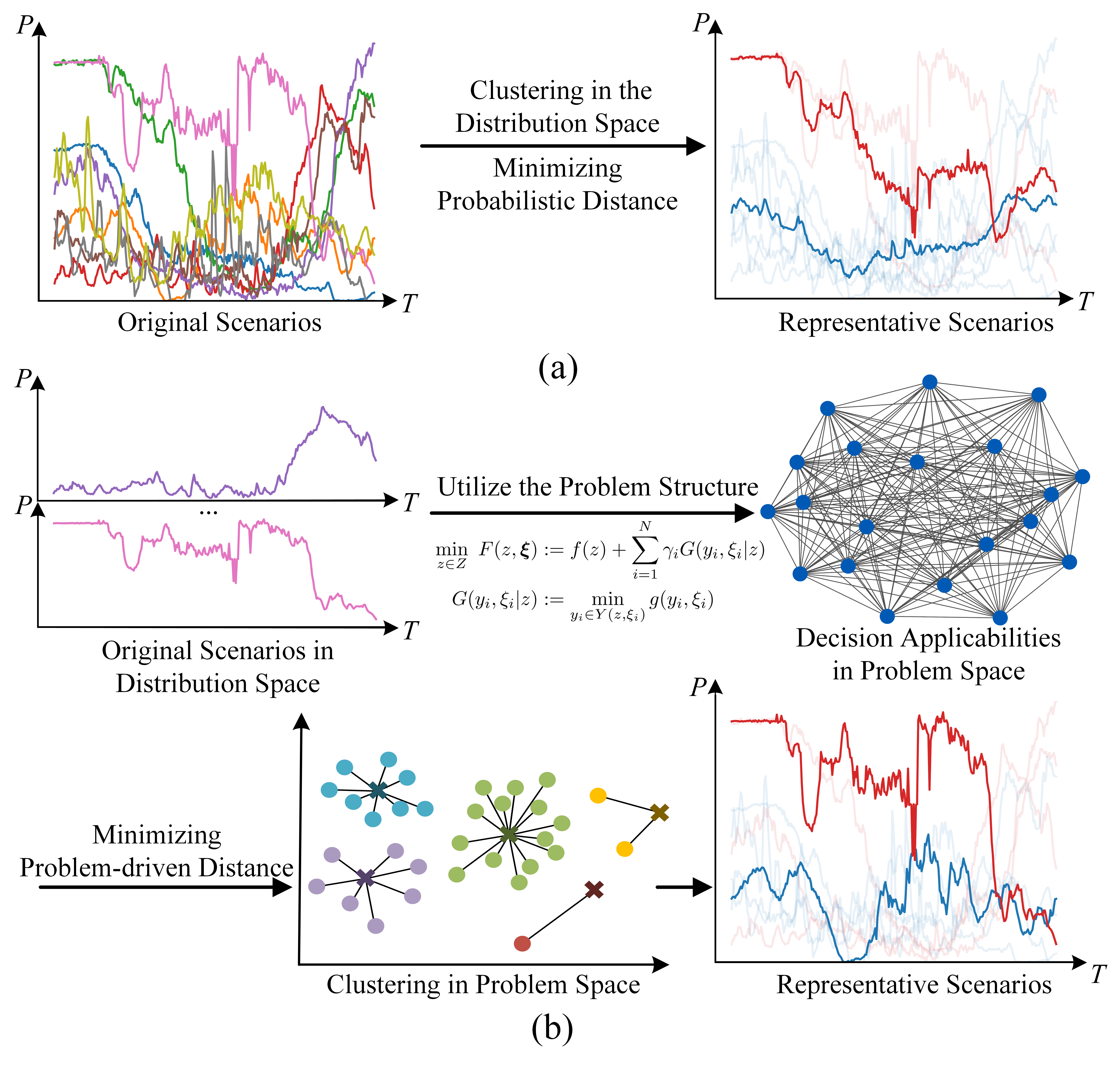
Figure 1: Diagrams of scenario reduction methodologies: (a) distribution-driven scenario reduction and (b) problem-driven scenario reduction.

To address this gap, SR methods should re-evaluate representativeness of scenarios. Specifically, the efficacy of SR should be gauged by the performance of the representative scenarios with consideration of the SBSO problem structure, i.e., in problem space, as illustrated in Fig. 1(b). This paper, therefore, focuses on identifying scenarios with high decision applicability, which refers to their relatively large impacts on the optimal objective value and decision-making. Recently, literature has employed decision applicability into the SR process and denote the framework problem-dependent SR. In [23], a problem-dependent methodology is proposed for SR that relies on a computationally complex Wasserstein distance metric and alternating minimization algorithm, which limits scalability. A symmetric opportunity cost is employed in [24] as the distance metric to measure the decision applicability between scenarios, and heuristic methods are used to perform SR, which limits the ability to characterize the optimality gap. Ref. [25] interestingly develops a problem-driven scenario clustering method with asymmetric distance metric where the representative scenarios are selected based on their average decision applicability in the entire cluster, which limits scalability of the method to SBSOs with few scenarios and is impractical in power system applications.

In this paper, we propose a novel problem-driven scenario reduction (PDSR) framework for solving SBSO problems to near-optimality and case studies illustrate improvements of up to ten times in terms of scalability and optimality gap over seven state-of-the-art methods, which enables PDSR applications to power systems for the first time. Specifically, our contributions are as follows:

1. Problem-Driven Scenario Reduction Framework: We propose a novel PDSR framework for general SBSO problems by defining the concept of optimality gap (OG) for SR and analytically characterizing the impacts of SR on the SBSO problem.

2. Problem-Driven Distance Metric: To evaluate the representativeness of scenarios, we introduce a provably effective problem-driven distance (PDD) metric that quantifies the mutual decision applicability between scenarios. We show that the OG can be bounded above by minimizing the sum of PDD within clusters (SPDD). Furthermore, we use the PDD to introduce new ex-ante and ex-post problem-driven SR evaluation indices.

3. Clustering Methodology: Based on the PDD, we convert the original scenario set partitioning and representative scenario selection processes into a mixed-integer linear program (MILP). The MILP objective balances minimization of SPPD within clusters and the total number of clusters (i.e., representative scenarios).

4. Simulation-based Analysis: A 24-hour, active distribution network (ADN) case study validates the presented PDSR framework by applying it to a stochastic economic dispatch problem, which co-optimizes day-ahead and intraday market participation by trading off energy storage capacity procurement and curtailment of renewable generation and load. Simulation results demonstrate PDSR’s ability to identify salient scenarios that achieve an SR optimality gap up to ten times smaller than the seven state-of-the-art SR methods.

The remainder of the paper is organized as follows. Section II introduces the proposed PDSR framework. Formulation of a scenario-based stochastic economic dispatch problem for an active distribution network is presented in Section III. Numerical studies based on real-world data are provided in Section IV to illustrate comparative performance. Finally, conclusions are summarized in Section V.

II Problem-Driven Scenario Reduction
Framework

In this section, we detail the novel PDSR framework within the context of a general two-stage stochastic optimization (TSSO) problem, which represents a rich set of power system problems. Note that the PDSR framework can be adapted to single-stage and multi-stage SBSO problems.

II-A Formulation of Two-Stage Stochastic Optimization

Two-stage stochastic optimization is an effective formulation in stochastic optimization to address uncertainties due to its “here-and-now” and “wait-and-see” characteristics, which respectively represent the decisions to be made before and after the uncertainty is revealed. The general formulation of the TSSO built on the original scenario set is

$$\min\limits_{z\in Z}\ F(z,\bm{\xi}) :=f(z)+\sum\nolimits_{i=1}^{N}\gamma_{i}G(y_{i},\xi_{i}|z)$$ (1a)

$$G(y_{i},\xi_{i}|z) :=\min\limits_{y_{i}\in Y(z,\xi_{i})}g(y_{i},\xi_{i}),$$ (1b)

where $F(z,\bm{\xi})$ is the objective function of the TSSO, including the cost of the first stage and the expected cost of the second stage. The original set of $N$ scenarios is denoted as $\bm{\xi}=\{\xi_{1},\xi_{2},...,\xi_{N}\}$ and $f(z)$ is the objective function of the first stage with the decision variable $z\in Z$. Here, $Z\subseteq R^{n}$ denotes the bounded feasible set. The second-stage problem is $G(y_{i},\xi_{i}|z)$ under the uncertainty $\xi_{i}$ with $y_{i}\in Y(z,\xi_{i}),Y\subseteq R^{m}$ as the decision variable and $z$ as the parameter. $g(y_{i},\xi_{i})$ is the objective function of the second stage. The probability of scenario $\xi_{i}$ is $\gamma_{i}\geq 0$, which satisfies $\sum_{i=1}^{N}\gamma_{i}=1$. We denote the optimal solution of (1) as $z^{\ast}_{\bm{\xi}}=\underset{z\in Z}{{\arg\min}}\ F(z,\bm{\xi})$. Additionally, we denote $F(z,\xi_{i}):=f(z)+G(y_{i},\xi_{i})$ with $z_{\xi_{i}}^{\ast}=\underset{z\in Z}{{\arg\min}}\ F(z,\xi_{i})$. We have $F(z,\bm{\xi})=\sum_{i=1}^{N}\gamma_{i}F(z,\xi_{i})$. We reasonably require the TSSO to satisfy the assumption of relatively complete recourse, implying that there exists a solution to TSSO for any $z\in Z$ and $\xi\in\bm{\xi}$. This assumption is common in stochastic optimization, ensuring sufficient resources to handle potential risks, even costly.

To address the challenges of computation complexity when $N$ is large, SR is employed to significantly reduce the computation complexity while maintaining the problem optimality approximation accuracy at an acceptable level. The SR process can be denoted as $\bm{C}(\bm{\xi},K)=\{\{C_{1},...,C_{K}\}:C_{i}\neq\emptyset,\forall i;C_{i}\cap C_{j}=\emptyset,\forall i\neq j;\cup_{i}C_{i}=I,I=\{1,\ldots,N\}\}$. The original scenario set $\bm{\xi}$ is partitioned into $K(K\ll N)$ clusters and is reduced to a representative scenario set $\bm{\zeta}=\{\zeta_{1},\zeta_{2},...,\zeta_{K}\}$. Each scenario cluster $C_{k}$ is represented by the representative scenario $\zeta_{k}$ with corresponding weight $\omega_{k}=\sum_{i\in C_{k}}\gamma_{i}$, which satisfies $\sum_{k=1}^{K}\omega_{k}=1$. In this paper, we concentrate on selecting $\bm{\zeta}$ as a subset of $\bm{\xi}$, instead of generating new scenarios. The TSSO formulated on the representative scenario set $\bm{\zeta}$ is given by

$$\min\limits_{z\in Z}\ \tilde{F}(z,\bm{\zeta}) :=f(z)+\sum\nolimits_{k=1}^{K}\omega_{k}G(y_{k},\zeta_{k}|z)$$ (2a)

$$G(y_{k},\zeta_{k}|z) :=\min\limits_{y_{k}\in Y(z,\zeta_{k})}g(y_{k},\zeta_{k}).$$ (2b)

The optimal solution of the reduced problem (2) is denoted as $z^{\ast}_{\bm{\zeta}}=\underset{z\in Z}{{\arg\min}}\ \tilde{F}(z,\bm{\zeta})$. Specifically, we would like to understand how SR affects the optimality of SBSO. Thus, we seek to define an SR optimality gap metric next.

II-B SR Optimality Gap

SR aims to minimize the optimality gap from using $K$ representative ($\bm{\zeta}$) vs. $N$ scenarios ($\bm{\xi}$). Towards this purpose, the OG can be defined as

$$OG:=F(z^{\ast}_{\bm{\zeta}},\bm{\xi})-F(z^{\ast}_{\bm{\xi}},\bm{\xi}),$$ (3)

where $F(z^{\ast}_{\bm{\zeta}},\bm{\xi})$ means solving (1) with $z=z^{\ast}_{\bm{\zeta}}$. Compared to [25], we present a distinct and rigorous derivation of an upper bound on OG.

Since $F(z,\bm{\xi})\geq F(z^{\ast}_{\bm{\xi}},\bm{\xi})$ for all $z\in Z$, we have $OG\geq 0$. A smaller $OG$ indicates a more accurate problem optimality approximation of $\bm{\zeta}$ to $\bm{\xi}$. Since $\tilde{F}(z,\bm{\zeta})\geq\tilde{F}(z^{\ast}_{\bm{\zeta}},\bm{\zeta})$ for all $z\in Z$, we can derive an upper bound of $OG$ as

$$\begin{split}OG\leq&F(z^{\ast}_{\bm{\zeta}},\bm{\xi})-F(z^{\ast}_{\bm{\xi}},\bm{\xi})+(\tilde{F}(z^{\ast}_{\bm{\xi}},\bm{\zeta})-\tilde{F}(z^{\ast}_{\bm{\zeta}},\bm{\zeta}))\\ =&(F(z^{\ast}_{\bm{\zeta}},\bm{\xi})-\tilde{F}(z^{\ast}_{\bm{\zeta}},\bm{\zeta}))-(F(z^{\ast}_{\bm{\xi}},\bm{\xi})-\tilde{F}(z^{\ast}_{\bm{\xi}},\bm{\zeta})).\\ \end{split}$$ (4)

Note that both the first and the last pair of terms share a common expression of $F(z,\bm{\xi})-\tilde{F}(z,\bm{\zeta})$, which can be further reformulated as

$$F(z,\bm{\xi})-\tilde{F}(z,\bm{\zeta})= \sum_{i=1}^{N}\gamma_{i}F(z,\xi_{i})-\sum_{k=1}^{K}\omega_{k}F(z,\zeta_{k})$$

$$= \sum_{k=1}^{K}\sum_{i\in C_{k}}\gamma_{i}F(z,\xi_{i})-\sum_{k=1}^{K}\sum_{i\in C_{k}}\gamma_{i}F(z,\zeta_{k})$$

$$= \sum_{k=1}^{K}\sum_{i\in C_{k}}\gamma_{i}\bigl{(}F(z,\xi_{i})-F(z,\zeta_{k})\bigr{)}.$$ (5)

Combining (4) and (5), the upper bound of $OG$ can be further expanded as

$$\begin{split}OG\leq\sum\nolimits_{k=1}^{K}\sum\nolimits_{i\in C_{k}}&\gamma_{i}\bigl{(}F(z^{\ast}_{\bm{\zeta}},\xi_{i})-F(z^{\ast}_{\bm{\zeta}},\zeta_{k})\bigr{)}\\ \quad-\sum\nolimits_{k=1}^{K}\sum\nolimits_{i\in C_{k}}&\gamma_{i}\bigl{(}F(z^{\ast}_{\bm{\xi}},\xi_{i})-F(z^{\ast}_{\bm{\xi}},\zeta_{k})\bigr{)}\\ \leq\sum\nolimits_{k=1}^{K}\sum\nolimits_{i\in C_{k}}&\gamma_{i}\bigl{(}|F(z^{\ast}_{\bm{\zeta}},\xi_{i})-F(z^{\ast}_{\bm{\zeta}},\zeta_{k})|\\ &\ +|F(z^{\ast}_{\bm{\xi}},\xi_{i})-F(z^{\ast}_{\bm{\xi}},\zeta_{k})|\bigr{)}.\\ \end{split}$$ (6)

Given that $z^{\ast}_{\bm{\xi}}$ and $z^{\ast}_{\bm{\zeta}}$ are not known, we use result from [26] to derive an upper bound on (6) based on (7), which states that for a locally Lipschitz continuous function $F(z,\xi)$, there exists a continuous symmetric function $d(\cdot)$ and a non-decreasing function $h(\cdot)$, such that for each $z\in Z$ and $\xi_{i},\zeta_{k}\in\bm{\xi}$, we have

$$|F(z,\xi_{i})-F(z,\zeta_{k})|\leq h(\|z\|)d(\xi_{i},\zeta_{k}),$$ (7)

where $d(\xi_{i},\zeta_{k})$ is required to satisfy the following properties:

C1) Consistency: $d(\zeta_{k},\xi_{i})=0\Leftrightarrow\zeta_{k}=\xi_{i}$;

C2) Symmetricity: $d(\zeta_{k},\xi_{i})=d(\xi_{i},\zeta_{k})$, $\forall\zeta_{k},\xi_{i}\in\bm{\xi}$;

C3) Convergence: $\sup\{d(\zeta_{k},\xi_{i}):\zeta_{k},\xi_{i}\in\bm{\xi},\|\zeta_{k}-\xi_{i}\|\leq\delta\}$ tends to 0 as $\delta\rightarrow 0$;

C4) Triangle inequality: $\exists$ measurable, bounded function $\lambda(\cdot)$, where $d(\zeta_{k},\xi_{i})<\lambda(\zeta_{k})+\lambda(\xi_{i})$.

Finally, combining (6) and (7) begets

$$\begin{split}OG\leq&(h(\|z^{\ast}_{\bm{\xi}}\|)+h(\|z^{\ast}_{\bm{\zeta}}\|))\sum\nolimits_{k=1}^{K}\sum\nolimits_{i\in C_{k}}\gamma_{i}d(\xi_{i},\zeta_{k}).\end{split}$$ (8)

Now, the primary challenge to apply the above result lies in defining an appropriate distance metric in the problem space, $d(\xi_{i},\zeta_{k})$, that satisfies properties C1)-C4). Note that since that $Z$ is bounded, $\|z\|$ is well-defined, i.e, $\exists M\gg 1,~{}\|z\|\leq M~{}\forall\,z\in Z$. Next, we construct the problem space and then define an appropriate metric $d(\xi_{i},\zeta_{k})$ within the problem space.

II-C Problem Space Transformation

In scenario-based problem formulations, each $z^{\ast}_{\zeta_{k}}$ is usually implemented within its respective scenario clusters. We denote $z_{\zeta_{k}}^{\ast}=\underset{z\in Z}{{\arg\min}}\ F(z,\zeta_{k})$. Motivated by this, our framework transforms the original scenario set in the distribution space into the problem space, which is constructed by the decision applicability between scenarios. The transformation process can be denoted as $\bm{\xi}\rightarrow\bm{F}$, where $\bm{F}:=\{F_{ij}=F(z_{\xi_{i}}^{\ast},\xi_{j})\mid i,j\in I\}$. Each $F_{ij}$ is a scenario-specific problem and is bounded under the condition of relatively complete recourse. In this way, we can directly quantify the impacts of uncertainty and systematically incorporate the inherent characteristics of the SBSO problem into the SR process. Of course, this approach necessitates solving $N^{2}$ optimization problems to determine $\bm{F}$, which may be computationally intensive for large $N$. However, since each problem is independent and can be solved in parallel, the absolute time required to find $F$ can be reduced significantly. The algorithmic efficiency is analyzed in IV-C.

II-D Problem-Driven Distance Metric

One way to describe the decision applicability is to use the opportunity cost, which pertains to the trade-off wherein the selection of a particular action necessitates the relinquishment of potential benefits associated with the best alternative. In the context of SR, when we choose scenario $\zeta_{k}$ to represent scenario $\xi_{i}$, the opportunity cost is defined as

$$c(\zeta_{k},\xi_{i}):=F(z_{\zeta_{k}}^{\ast},\xi_{i})-F(z_{\xi_{i}}^{\ast},\xi_{i}).$$ (9)

However, $c(\zeta_{k},\xi_{i})$ does not satisfy all properties C1)-C4) and cannot serve as distance metric, $d(\cdot)$. Instead, we consider the following problem-driven distance metric between scenarios $\xi_{i}$ and $\zeta_{k}$:

$$d(\xi_{i},\zeta_{k}):= c(\zeta_{k},\xi_{i})+c(\xi_{i},\zeta_{k})$$ (10)

$$= F(z_{\zeta_{k}}^{\ast},\xi_{i})-F(z_{\xi_{i}}^{\ast},\xi_{i})+F(z_{\xi_{i}}^{\ast},\zeta_{k})-F(z_{\zeta_{k}}^{\ast},\zeta_{k}).$$

Proposition 1.

The distance metric $d(\xi_{i},\zeta_{k})$ in (10) satisfies all four properties C1)-C4) for (7).

Proof.

Please see proof in Appendix -A. ∎

The PDD metric in (10) effectively quantifies the mutual decision applicability between two scenarios. That is, a small $d(\xi_{i},\zeta_{k})$ implies that scenario $\zeta_{k}$ can accurately represent scenario $\xi_{i}$.

Combining (8) and (10) begets

$$\begin{split}OG\leq 2h(M)\sum\nolimits_{k=1}^{K}\sum\nolimits_{i\in C_{k}}\gamma_{i}&\bigl{(}F(z_{\zeta_{k}}^{\ast},\xi_{i})-F(z_{\xi_{i}}^{\ast},\xi_{i})\\ +&F(z_{\xi_{i}}^{\ast},\zeta_{k})-F(z_{\zeta_{k}}^{\ast},\zeta_{k})\bigr{)}.\end{split}$$ (11)

Note that while the above analysis extends to non-convex formulations in (2), it is conditioned on finding the global optimum $z^{\ast}$. That is, convexity in (2) guarantees that bounds on $OG$ hold and is the focus of this paper. Next, we select salient scenarios that minimize the upper bound in (11).

II-E MILP Reformulation of Clustering

Since $2h(M)$ in (11) is a constant, minimizing the sum of PDD within clusters achieves the lowest upper bound of OG. To achieve this, the processes of scenarios partitioning and representative scenarios selection can be rendered as the following MILP formulation.

$$\min_{v,u,l,K} \ \sum\nolimits_{j=1}^{N}\ l_{j}+\beta K/{N}$$ (12a)

s.t. $$\sum\nolimits_{i=1}^{N}\gamma_{i}v_{ij}(F_{ji}-F_{ii}+F_{ij}-F_{jj})\leq l_{j},\ \forall j\in I$$ (12b)

$$v_{ij}\leq u_{j},\ v_{jj}=u_{j},\ \forall i,j\in I$$ (12c)

$$\sum\nolimits_{j=1}^{N}v_{ij}=1,\ \forall i\in I$$ (12d)

$$\sum\nolimits_{j=1}^{N}u_{j}=K$$ (12e)

In (12a), $\sum_{j=1}^{N}\ l_{j}$ describes the SPDD, and $K/N$ describes the reduction degree. $\beta$ is the trade-off factor to achieve a balance between the SPDD and reduction degree, while simultaneously deciding the optimal clustering number $K$. The binary variable $u_{j}$ indicates whether scenario $\xi_{j}$ is selected as a representative scenario of a cluster, while the binary variable $v_{ij}$ determines whether scenario $\xi_{i}$ is included in the cluster represented by scenario $\xi_{j}$. Constraint $v_{ij}\leq u_{j}$ ensures that $\xi_{i}$ can only be assigned to a cluster that has a designated representative, while $v_{jj}=u_{j}$ enforces that $\xi_{i}$ must be assigned to its own cluster if it’s a representative scenario. Constraint (12d) ensures that each scenario $\xi_{j}$ can only be assigned to one cluster, while (12e) guarantees that exactly $K$ clusters are formed. The weight of each cluster is calculated as $\omega_{k}=\sum_{i=1}^{N}v_{ik}\gamma_{i}$.

II-F Problem-Driven Evaluation Indices

In this section, two types of problem-driven evaluation indices are introduced: ex-ante and ex-post indices. Ex-ante indices emphasizes the SR’s ability in partitioning and representing the original scenario set in the problem space before solving the reduced problem. Ex-post indices focus on the impacts of SR on the outcomes of the TSSO after solving the reduced problem. For the following indices, the first three indices are classified as ex-ante indices, while the last two indices are ex-post indices.

II-F1 Sum of PDD within clusters (SPDD)

$$\text{SPDD}:=\sum_{j=1}^{N}\ l_{j}=\sum_{k=1}^{K}\sum_{i\in C_{k}}\gamma_{i}(F_{ki}-F_{ii}+F_{ik}-F_{kk}).$$ (13)

SPDD measures the dispersion between scenarios and their respective clusters. A smaller SPDD value indicates a tighter clustering result in the problem space.

II-F2 Problem-Driven Davies-Bouldin Index

Based on the Davies-Bouldin Index, we introduce the Problem-driven Davies-Bouldin Index (PDDBI) utilizing the PDD:

PDDBI $$:=\frac{1}{K}\sum_{m=1}^{K}\max_{1\leq n\neq m\leq K}\bigl{(}\frac{D_{m}+D_{n}}{d(\zeta_{m},\zeta_{n})}\bigr{)}$$ (14a)

$$D_{m} :=\sum_{i\in C_{m}}\frac{\gamma_{i}}{\omega_{m}}d(\zeta_{m},\xi_{i}).$$ (14b)

A smaller PDDBI value indicates a better quality of the balance between the within-cluster compactness and the between-cluster separation.

II-F3 Cluster decision similarity

PDSR underscores the emphasis on high strategy adaptability, which often aligns with similar strategies within the same cluster. Noted that clustering solely based on strategy similarity, as one of the DDSR methods, can not guarantee high strategy adaptability. We denote $sim(z_{\xi_{i}}^{\ast},z_{\xi_{j}}^{\ast})$ as the similarity between $z_{\xi_{i}}^{\ast}$ and $z_{\xi_{j}}^{\ast}$, and determine the decision similarity of the cluster $C_{k}$ as

$$S_{C_{k}}:=\sum_{i\in C_{k}}\sum_{j\in C_{k}}\frac{\gamma_{i}\gamma_{j}}{\omega_{k}^{2}}sim(z_{\xi_{i}}^{\ast},z_{\xi_{j}}^{\ast}).$$ (15)

$\bar{S}_{C}=\frac{1}{K}\sum_{k=1}^{K}S_{C_{k}}$ denotes the average cluster decision similarity of all clusters. The selection of $sim(\cdot)$ depends on the nature of decision variables. For instance, cosine similarity can be employed for continuous decision variables, while normalized Euclidean distance is a suitable choice for decision variables within intervals.

II-F4 Optimality gap

After solving (1) and (2), we apply $z^{\ast}_{\bm{\xi}}$ and $z^{\ast}_{\bm{\zeta}}$ to $\bm{\xi}$, and calculate the percentage value of OG as

$$OG_{\bm{\zeta}}(\%):=\bigl{(}F(z^{\ast}_{\bm{\zeta}},\bm{\xi})-F(z^{\ast}_{\bm{\xi}},\bm{\xi})\bigr{)}/{F(z^{\ast}_{\bm{\xi}},\bm{\xi})}.$$ (16)

This metric indicates the percentage deviation of the approximated optimality from the optimality of the original problem, and is desired to be close to zero .

II-F5 Representative scenario effectiveness

For the SBSO based on the representative scenarios, identifying the relative importance of individual representative scenario is crucial for comprehending the problem structure and making reasonable decisions. We introduce the concept of “Scenario Effectiveness”, measuring the significance of a given representative scenario in the problem space. The scenario effectiveness of scenario $\zeta_{k}$, denoted as $SE_{\zeta_{k}}(\%)$, is characterized by the changes in the percentaged OG upon its removal from $\bm{\zeta}$:

$$SE_{\zeta_{k}}(\%):=OG_{\bm{\zeta}_{-k}}(\%)-OG_{\bm{\zeta}}(\%),$$ (17)

where $\bm{\zeta}_{-k}=\bm{\zeta}\setminus\{\zeta_{k}\}$. A higher value of $SE_{\zeta_{k}}(\%)$ signifies that the removal of $\zeta_{k}$ induces more substantial changes in the OG. This indicates that $\zeta_{k}$ holds greater significance in influencing the reduced problem outcomes.

The proposed PDSR framework is illustrated in Algorithm 1. To illustrate the effectiveness of the proposed PDSR framework, we consider the following two-stage stochastic economic dispatch problem.

Input: Scenario set $\bm{\xi}$ of $N$ scenarios and weights $\bm{\gamma}$.

Output: Scenario set $\bm{\zeta}$ of $K$ scenarios and weights $\bm{\omega}$.

Step 1 - Transformation in Problem Space

       Step 1.1: Initialize problem space matrix $\bm{F}=\mathbf{0}$.;

       Step 1.2: Transform the distribution space into
problem space by:;

      

      for $i=1$ to $N$  do

             Solve the scenario-specific TSSO problem
$F(z,\xi_{i})$ and obtain the optimal decision $z_{\xi_{i}}^{\ast}$. ;

             Set $F_{ii}=F(z_{\xi_{i}}^{\ast},\xi_{i})$.;

             for $j=1$ to $N$, $i\neq j$ parallel do

                   Solve the single-stage and deterministic
problem $G(y_{j},\xi_{j}|z_{\xi_{i}}^{\ast})$ in (1b).;

                   Set $F_{ij}=F(z_{\xi_{i}}^{\ast},\xi_{j})$.

             end for

            

       end for

      

Step 2 - Clustering

      

      Step 2.1: Select $\beta$ in (12a) from ex-ante indices.;

       Step 2.2: Solve MILP in (12) to obtain the
representative scenario set $\bm{\zeta}$ with weights $\bm{\omega}$.;

      

Algorithm 1 Problem-Driven Scenario Reduction

III Two-Stage Stochastic Economic Dispatch for Active Distribution Networks

In this section, we consider an optimal stochastic economic dispatch of an ADN that trades with the transmission system. The ADN’s assets include wind turbines (WT), photovoltaic system (PV) and energy storage (ES) facilities. We will focus on uncertainties from WT, PV, loads and two electricity markets: day-ahead and intraday prices [27], which engenders the two stages for dispatch. In the day-ahead stage, uncertainties are addressed using the representative scenario set and the ADN needs to sign contracts for power trading with the transmission system operator and procure ES capacity from the ES owner. In the intraday stage, due to the uncertainties, there will exist deviations between the scheduled day-ahead power trading and the actual intraday power demand, and even violations of safety constraints especially in worst-case scenarios. Therefore, the ADN decision-maker is risk-averse and prefers to limit constraint violations, which are mainly considered as voltage magnitude constraint violations.

III-A Objective Function

In the day-ahead stage, the objective is to minimize the total operation cost including the day-ahead trading cost and the expected intraday balancing cost and penalty cost. The day-ahead trading cost in (18b) includes the cost of trading power with transmission system and the procurement of ES capacity. The intraday cost includes the balancing cost in the intraday balancing market in (18c), and the penalty cost of load shedding and RES curtailment in (18d).

$$\min\ C^{\mathrm{DA}}+C^{\mathrm{IN,im}}+C^{\mathrm{IN,p}}$$ (18a)

$$C^{\mathrm{DA}}=\sum_{s=1}^{S}{\omega_{s}}\sum_{t=1}^{T}{\pi_{s,t}^{\mathrm{T}}P_{t}^{\mathrm{T}}\Delta t}+\sum_{j\in\varOmega_{\mathrm{E}}}\pi_{j}^{\mathrm{E}}E_{j}$$ (18b)

$$C^{\mathrm{IN,im}}=\sum_{s=1}^{S}{\omega_{s}}\sum_{t=1}^{T}\Delta t(\pi_{s,t}^{\mathrm{T}+}P_{s,t}^{\mathrm{T}+}+\pi_{s,t}^{\mathrm{T}-}P_{s,t}^{\mathrm{T}-})$$ (18c)

$$C^{\mathrm{IN,p}}=\sum_{s=1}^{S}\omega_{s}\sum_{t=1}^{T}\Delta t(\mkern-4.0mu\sum_{j\in\varOmega_{\mathrm{R}}}\pi^{\mathrm{R},\mathrm{c}}P_{j,s,t}^{\mathrm{R},\mathrm{c}}+\mkern-6.0mu\sum_{j\in\varOmega_{\mathrm{L}}}\pi^{\mathrm{L},\mathrm{s}}P_{j,s,t}^{\mathrm{L},\mathrm{s}}).$$ (18d)

$\pi_{s,t}^{\mathrm{T}}$ and $P_{t}^{\mathrm{T}}$ are the trading electricity price and trading power between the ADN and transmission system in the day-ahead market, respectively. $\pi_{j}^{\mathrm{E}}$ and $E_{j}$ are the procurement price and procured ES capacity at bus $j$. $T$ and $\Delta t$ are time period and time interval for scheduling. $S$ is the number of scenarios and $\omega_{s}$ is the weight of scenario $s$. $\pi_{s,t}^{\mathrm{T}+}/\pi_{s,t}^{\mathrm{T}-}$ are the imbalancing price of up-regulation and down-regulation in the intraday balancing market under scenario $s$ and time $t$. $P_{s,t}^{\mathrm{T}+}/P_{s,t}^{\mathrm{T}-}$ are the imbalanced purchasing and selling power in the intraday balancing market. In the intraday balancing market, the ADN can only purchase balancing energy at a higher price than in the day-ahead market, while selling electricity at a lower price. $P_{j,s,t}^{\mathrm{R},\mathrm{c}}/P_{j,s,t}^{\mathrm{L},\mathrm{s}}$ are the power of RES curtailment and load shedding at bus $j$. $\varOmega_{\mathrm{R}}/\varOmega_{\mathrm{L}}/\varOmega_{\mathrm{E}}$ refer to the set of buses of RES, load, and ES. $\pi^{\mathrm{R},\mathrm{c}}/\pi^{\mathrm{L},\mathrm{s}}$ are the penalty cost of RES curtailment and load shedding.

III-B Operational Constraints

III-B1 Power flow constraints

The linear version of the DistFlow model, i.e., LinDistFlow [28] is used in this paper to approximate nodal voltage magnitudes and active/reactive line flows in the ADN with the assumption that line losses can be neglected. For $\forall j\in\varOmega_{\mathrm{B}}$, we have

$$V_{j,s,t}^{2}=V_{i,s,t}^{2}-2(r_{ij}P_{ij,s,t}+x_{ij}Q_{ij,s,t})$$ (19a)

$$p_{j,s,t}=P_{ij,s,t}-\sum_{l:j\rightarrow l}P_{jl,s,t}$$ (19b)

$$q_{j,s,t}=Q_{ij,s,t}-\sum_{l:j\rightarrow l}Q_{jl,s,t}$$ (19c)

$$\underline{V_{j}}\leq V_{j,s,t}\leq\overline{V_{j}},$$ (19d)

where $r_{ij}/x_{ij}$ are the line resistance/reactance between bus $i$ and $j$, respectively. $V_{j,s,t}$ is the voltage at bus $j$ for scenario $s$ at time $t$. $P_{ij,s,t}/Q_{ij,s,t}$ are the line active/reactive power between bus $i$ and $j$, respectively. $p_{j,s,t}/q_{j,s,t}$ are the active/reactive injection power at bus $j$. (19a) describes the voltage drop over branch from bus $i$ to bus $j$. (19b) and (19c) represent the active and reactive power balance at bus $j$. (19d) describes voltage magnitude limits at bus $j$, with $\overline{V_{j}}/\underline{V_{j}}$ as the upper/lower bound of voltage magnitude.

III-B2 RES curtailment and load shedding constraints

For $\forall j\in\varOmega_{\mathrm{R}}$, we have

$$0\leq P_{j,s,t}^{\mathrm{R},\mathrm{c}}\leq P_{j,s,t}^{\mathrm{R}}$$ (20a)

$$0\leq P_{j,s,t}^{\mathrm{L},\mathrm{s}}\leq P_{j,s,t}^{\mathrm{L}},$$ (20b)

where $P_{j,s,t}^{\mathrm{R}}/P_{j,s,t}^{\mathrm{L}}$ are the RES injection/active power consumption at bus $j$ for scenario $s$ at time $t$, respectively.

III-B3 ES operation constraints

For $\forall j\in\varOmega_{\mathrm{E}}$, we have

$$SoC_{j,s,t+1}=SoC_{j,s,t}+\Delta t(P_{j,s,t}^{\mathrm{E},\mathrm{c}}\eta_{j}^{\mathrm{c}}-P_{j,s,t}^{\mathrm{E},\mathrm{d}}/\eta_{j}^{\mathrm{d}})/E_{j}$$ (21a)

$$\sum\nolimits_{t=1}^{T}(P_{j,s,t}^{\mathrm{E},\mathrm{c}}\eta_{j}^{\mathrm{c}}-P_{j,s,t}^{\mathrm{E},\mathrm{d}}/\eta_{j}^{\mathrm{d}})\Delta t=0$$ (21b)

$$0\leq P_{j,s,t}^{\mathrm{E},\mathrm{c}}\leq(1-D_{j,s,t}^{\mathrm{E}})\overline{P_{j}^{\mathrm{E}}}$$ (21c)

$$0\leq P_{j,s,t}^{\mathrm{E},\mathrm{d}}\leq D_{j,s,t}^{\mathrm{E}}\overline{P_{j}^{\mathrm{E}}}$$ (21d)

$$\underline{SoC}\leq SoC_{j,s,t}\leq\overline{SoC},$$ (21e)

where $P_{j,s,t}^{\mathrm{E},\mathrm{c}}/P_{j,s,t}^{\mathrm{E},\mathrm{d}}$ are the charge/discharge power. Constraints (21a)-(21b) and (21e) are related to the state of charge (SoC). $\overline{SoC}/\underline{SoC}$ denote the maximum/minimum SoC, respectively. $\eta_{j}^{\mathrm{c}}/\eta_{j}^{\mathrm{d}}$ are the charge/discharge efficiency, respectively. Constraint (21b) guarantees that the capacity at the last time period is equal to the initial capacity. Constraints (21c) and (21d) impose restrictions on the maximum charging and discharging power and charging state of ES. $D_{j,s,t}^{\mathrm{E}}$ is a binary variable indicating the charging/discharging state.

III-B4 Trading constraints with transmission system

$$0\leq P_{s,t}^{\mathrm{T}+}\leq(1-D_{s,t}^{\mathrm{T}})\overline{P^{\mathrm{T}}}$$ (22a)

$$0\leq P_{s,t}^{\mathrm{T}-}\leq D_{s,t}^{\mathrm{T}}\overline{P^{\mathrm{T}}}$$ (22b)

$$-\overline{P^{\mathrm{T}}}\leq P_{t}^{\mathrm{T}}+P_{s,t}^{\mathrm{T}+}-P_{s,t}^{\mathrm{T}-}\leq\overline{P^{\mathrm{T}}},$$ (22c)

where $\overline{P^{\mathrm{T}}}$ is the maximum trading power between ADN and transmission system. (22a) and (22b) indicate that the ADN can only be in one balancing state at one time, with $D_{s,t}^{\mathrm{T}}$ as the balancing state of ADN.

III-B5 Energy balancing constraints

$$p_{j,s,t}=P_{j,s,t}^{\mathrm{E},\mathrm{c}}-P_{j,s,t}^{\mathrm{E},\mathrm{d}}+P_{j,s,t}^{\mathrm{L}}-P_{j,s,t}^{\mathrm{L},\mathrm{s}}-(P_{j,s,t}^{\mathrm{R}}-P_{j,s,t}^{\mathrm{R},\mathrm{c}})$$ (23a)

$$q_{j,s,t}=Q_{j,s,t}^{\mathrm{L}}-Q_{j,s,t}^{\mathrm{L},\mathrm{s}},$$ (23b)

where $Q_{j,s,t}^{\mathrm{L}}/Q_{j,s,t}^{\mathrm{L},\mathrm{s}}$ are the reactive power consumption and load shedding at bus $j$. We assume that all the RESs are of the unity power factor and the power factor of load demand remains the same after load shedding. $\forall~{}s,t$, if $j\notin\varOmega_{\mathrm{E}}$, $P_{j,s,t}^{\mathrm{E},\mathrm{c}}=P_{j,s,t}^{\mathrm{E},\mathrm{d}}=0$. Similarly, if $j\notin\varOmega_{\mathrm{R}}$, $P_{j,s,t}^{\mathrm{R}}=P_{j,s,t}^{\mathrm{R},\mathrm{c}}=0$.

Finally, the optimal day-ahead economic dispatch problem is formulated as (24), which is a mixed-integer linear problem, and can be solved by commercial solvers.

$$\begin{split}\min\ &C^{\mathrm{DA}}+C^{\mathrm{IN,im}}+C^{\mathrm{IN,p}}\\ s.t.\ &\eqref{pf}-\eqref{power balance}.\end{split}$$ (24)

IV Numerical Case Study

IV-A Problem Description

In this section, the proposed problem-driven scenario reduction framework is tested for two-stage stochastic economic dispatch in the modified IEEE 33-bus ADN. One WT is located at bus 10 and two PVs are located at buses 16 and 24, respectively. ES is located at bus 13. The voltage magnitude is restricted as $|V_{i}|\in[0.90,1.10]\ \text{(p.u.)},\ \forall i\in\varOmega_{\mathrm{B}}$. The time step is set as $\Delta t=15\min$ with $T=96$ steps. The original scenario set $\bm{\xi}$ comprises $N$ scenarios. It is worth mentioning that, to validate the performance of proposed PDSR framework in uncovering salient scenarios, particularly worst-case scenarios, we construct $\bm{\xi}$ by randomly selecting from historical observations, while also ensuring that it contains a specified number of bad scenarios [29]. Each individual scenario $\xi\in\mathbb{R}^{7T},~{}\xi\in\bm{\xi}$ is a multi-variable high-dimensional vector characterizing 7 sources of uncertainty. The capacities of WT and PVs are normalized to $1\mathrm{MW}$, $1.2\mathrm{MW}$ and $1\mathrm{MW}$. For simplicity, the intraday balancing market prices are set as $\pi_{s,t}^{\mathrm{T}+}=1.3\pi_{s,t}^{\mathrm{T}}$ and $\pi_{s,t}^{\mathrm{T}-}=0.7\pi_{s,t}^{\mathrm{T}}$. The power rating of ES is set as $0.4\mathrm{MW}/0.8\mathrm{MWh}$, and ES capacity procurement is limited by $E\leq 0.8\mathrm{MWh}$. The initial $SoC$ of ES is $0.5$ and $\eta^{\mathrm{c}}=\eta^{\mathrm{d}}=0.95$. The penalty costs of load shedding and RES curtailment are set as $\$1000/\mathrm{MWh}$ and $\$280/\mathrm{MWh}$, respectively. The TSSO problem built on $\bm{\xi}$ is used as the Benchmark. The optimization is coded in Python with the Yalmip interface and solved by Gurobi 11.0 solver. The programming environment is Intel Core i9-13900HX @ 2.30GHz with RAM 16 GB.

IV-B Performance of PDSR

First, we consider $N=400$ scenarios and construct the $\bm{F}$ matrix by solving $N^{2}$ scenario-specific deterministic problems. For all $F_{ij}$, the MIP-gap is $<10^{-4}$ (i.e., default Gurobi MIPGap), which ensures that the optimal solution is found. Then, we utilize the MILP formulation in (12) to decide $K$ through a comprehensive analysis of the normalized ex-ante indices under different $\beta$. The results are shown in Fig. 2. It is observed that $\beta=150$ and $K=7$ correspond to a local minimum in PDDBI alongside a relatively large $\bar{S}_{C}$, and the balance between reduction degree $K/N$ and SPDD is also achieved. It indicates that $7$ representative scenarios can provide the most favorable clustering structure for the dataset under analysis.

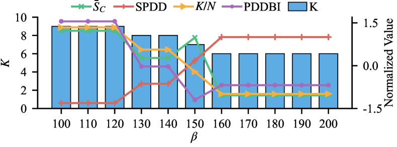
Figure 2: The ex-ante validity comparison of different $\beta$

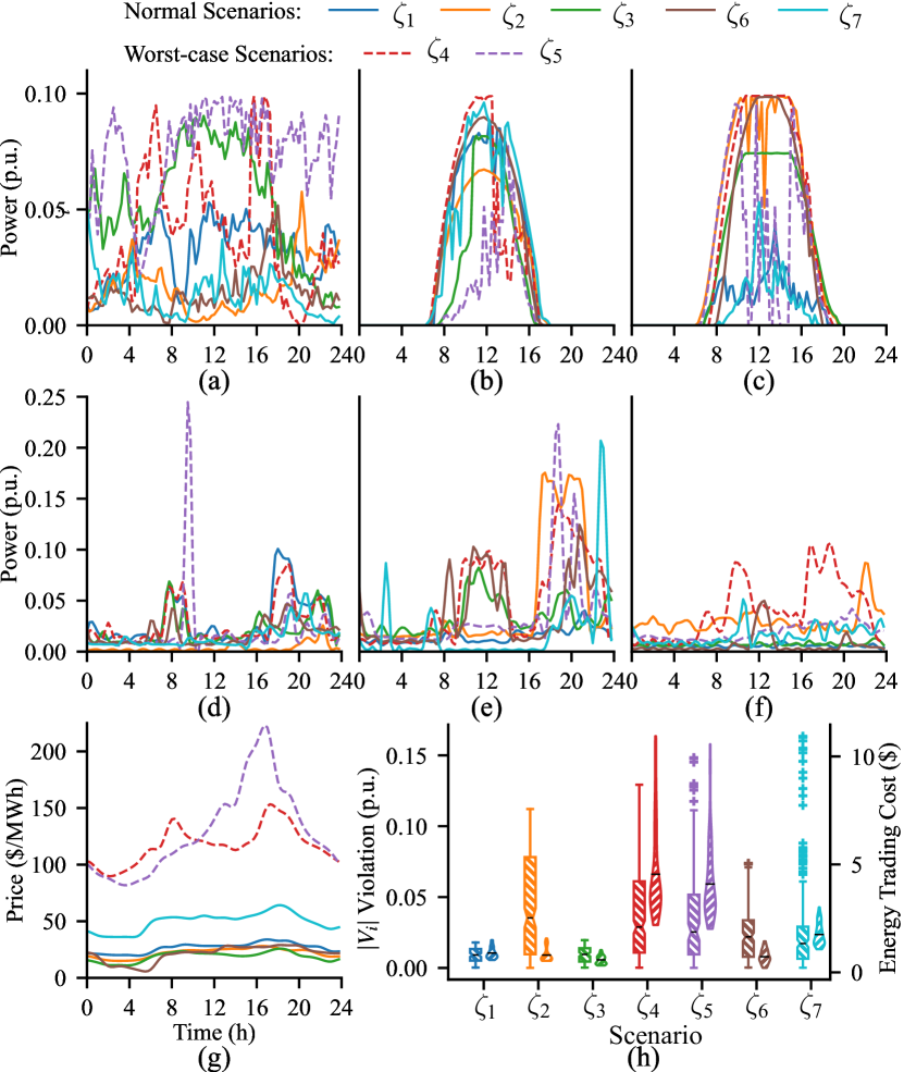
Figure 3: Representative scenarios obtained by the PDSR framework for $N=400$ and $K=7$: (a) WT at bus 10, (b) PV at bus 16, (c) PV at bus 24, (d) load at bus 10, (e) load at bus 16, (f) load at bus 24, (g) day-ahead electricity price and (h) un-optimization voltage magnitude violations (boxplot, left) and energy trading cost (violinplot, right) of the 7 representative scenarios from AC power flow.

The obtained $K=7$ representative scenario clusters of the proposed PDSR framework are presented in Fig. 3(a) to Fig. 3(g). Fig. 3(h) indicates the un-optimization voltage magnitude violations and energy trading cost of the 7 representative scenarios from AC power flow. This highlights the severity of these scenarios and underscores the importance of implementing reasonable dispatching practices. Curves in the same color belong to the same cluster. The corresponding weights of each cluster are $0.275$, $0.085$, $0.3025$, $0.0425$, $0.0525$, $0.1375$ and $0.105$, respectively. The representative scenarios in Fig. 3 illustrate PDSR’s effectiveness in identifying salient features from a large set of uncertainties in the system. Moreover, PDSR includes two worst-case scenarios (red $\zeta_{4}$ and purple $\zeta_{5}$) in the reduced set, where worst-case is based on top 5% decision adaptability rating defined as $\sum_{j=1}^{N}F(z_{\xi_{j}}^{\ast},\xi_{i})$ in the problem space. This metric describes the decision adaptability level of all other potential solutions to scenario $\xi_{i}$. Besides, their relatively small associated weight (only $0.0425$ and $0.0525$, indicating low occurrence probabilities), significant volatility and high values, and significant voltage magnitude violations and trading cost also verify them as worst-case scenarios. This observation is critical because incorporating too many worst-case scenarios into the representative scenario set may introduce conservatism, potentially leading to reduced economic efficiency.

The optimality gap $OG(\%)$ is $0.09\%$, which suggests a high level of approximation accuracy. We utilize the evaluation indices of cluster decision similarity and representative scenario effectiveness to further validate the performance of the proposed PDSR framework. In the two-stage stochastic economic dispatch problem of ADN, the similarity of power trading with transmission system is computed using cosine function, while the similarity in ES capacity procurement is calculated using normalized Euclidean distance. The results are illustrated in Table I.

TABLE I: Evaluation results of cluster decision similarity and representative scenario effectiveness for $N=400$ and $K=7$

	$C_{1}$	$C_{2}$	$C_{3}$	$C_{4}$	$C_{5}$	$C_{6}$	$C_{7}$
$S_{C_{k}}$	$0.920$	$0.983$	$0.981$	$0.938$	$0.922$	$0.933$	$0.928$
$SE_{\zeta_{k}}$	$0.14\%$	$0.19\%$	$0.12\%$	$0.35\%$	$0.50\%$	$0.12\%$	$0.22\%$

Table I indicates that the strategies across all clusters of the PDSR framework exhibit a notably high degree of similarity. This demonstrates that the PDSR framework has effectively grouped scenarios with similar operation strategies into the same cluster. Regarding the representative scenario effectiveness, Table I indicates that all the representative scenarios have a considerable impacts on the results of the problem. Notably, the scenario effectiveness of representative scenarios $\zeta_{4}$ and $\zeta_{5}$, corresponding to the red and purple curves in Fig. 3, are highlighted. This is consistent with the earlier analysis of the two scenarios being worst-case scenarios and important components of the representative scenario set.

IV-C Comparison with State-of-the-Art Methods

To further demonstrate the benefit of the proposed PDSR framework, we conduct a comparative analysis. DDSR methods including HC using Wasserstein distance (HC-W), $K$-means using Euclidean distances (KM-E), $K$-means using dynamic time warping distance (KM-D), and Gaussian mixture model using Mahalanobis distance (G-M) are compared. For DDSR methods incorporating relevant problem properties, we include $K$-means based on network power flow (KM-pf), and HC based on operational cost (HC-c) in comparison. Besides, we also include the method developed in ref. [24] with graph clustering (GC) for comparison. Additionally, the method of constructing the representative scenario set based on worst-case statistical indicators in the distribution space (WS) is included for comparison. The comparative indices include the number of worst-case scenarios captured in the representative scenario set $(\kappa)$, the $OG(\%)$ defined in (16), the ES capacity procurement $E$ from solving (2), the average penalty cost $\bar{C}^{\mathrm{IN,p}}$ from solving $F(z^{\ast}_{\bm{\zeta}},\xi)$ for all the $\xi\in\bm{\xi}$, the time required to process the data for clustering $(\tau_{\mathrm{p}})$, and the time required to solve the clustering problem $(\tau_{\mathrm{c}})$. The comparison results are presented in Table II.

TABLE II: Comparing SR methods for $N=400$ and $K=7$

Method	$\kappa$	$OG(\%)$	$E(\mathrm{MWh})$	$\bar{C}^{\mathrm{IN,p}}(\$)$	$\tau_{\mathrm{p}}(s)$	$\tau_{\mathrm{c}}(s)$
Benchmark	$20$	$0$	$0.44$	$632.4$	$-$	$-$
PDSR	$2$	$0.09$	$0.475$	$621.2$	$<0.3$	$2.74$
GC	$1$	$1.79$	$0.08$	$816.3$	$<0.3$	$0.21$
WS	$5$	$1.65$	$0.79$	$559.5$	$0.01$	$-$
HC-c	$0$	$2.69$	$0$	$860.1$	$86.31$	$0.01$
KM-pf	$0$	$2.63$	$0$	$859.9$	$86.31$	$0.78$
G-M	$0$	$2.51$	$0.01$	$852.0$	$-$	$6.96$
KM-D	$0$	$2.73$	$0$	$860.1$	$-$	$440.9$
KM-E	$0$	$2.66$	$0$	$860.1$	$-$	$0.31$
HC-W	$0$	$2.61$	$0$	$860.1$	$1.38$	$0.03$

SR Performance: The observations from Table II suggest that the PDSR framework, with a small value of $OG(\%)=0.09\%$, significantly outperforms other SR methods. Besides, the ES capacity procurement $E$ and $\bar{C}^{\mathrm{IN,p}}$ of PDSR also best approximate to the results of Benchmark. The DDSR methods, seeking for minimum statistical difference, fail to capture worst-case scenarios in their representative scenario sets, which leads to a neglect of potential risks during the operation, resulting in a zero procurement of ES capacity and an inability to cope with uncertainties, thus achieving relatively high penalty costs and $OG(\%)$. For instance, in heavy load situations, the bus voltage might drop below safety requirements. Without the support of ES, the ADN must resort to lots of load shedding to prevent violating the voltage safety constraints, thereby incurring substantial penalty cost. WS selects $7$ statistical worst-case scenarios in the distribution space, but only $5$ of them are real worst-case scenarios in the problem space. This discrepancy highlights that severity in statistical metrics does not necessarily equate to severity in problem outcomes. Moreover, focusing only on worst-case scenarios may result in overly conservative decisions and unnecessarily high costs. WS procures too much ES capacity as $E=0.79\mathrm{MWh}$, achieving a low penalty cost, which also leads to a relatively high $OG(\%)=1.65\%$. The GC method in ref. [24] captures 1 worst-case scenario with $OG(\%)=1.79\%$, which is much lower than the DDSR methods. This indicates that measuring the difference between scenarios by the symmetric opportunity cost can enhance the SR performance, but GC relies on heuristic methods to obtain the representative scenarios, potentially yielding suboptimal outcomes. Additionally, the method developed in [25] fails to solve the clustering process within 3 hours as their clustering methodology does not scale well with $N=400$. Compared to the above methods, the proposed PDSR framework efficiently considers the potential impacts of the scenarios on the problem, and include two reasonable worst-case scenarios in the representative scenario set, as analyzed in Section. IV-B. These comparative findings suggest that PDSR exhibits superior accuracy in representing the original scenario set, thereby offering more reliable information for decision-making in energy management under uncertainty.

Cluster Decision Similarity and Representative Scenario Effectiveness: The comparative results are illustrated in Fig. 4. Fig. 4(a) presents the comparative results of cluster decision similarity. We can see that the cluster decision similarity of DDSR methods and GC are substantially lower than those of PDSR. In Fig. 4(b), the comparative results of representative scenario effectiveness are depicted. For DDSR methods, the removal of any representative scenario does not have much impacts on the problem outcomes, whereas in PDSR, such a removal can significantly alter the problem outcomes. This indicates that the proposed PDSR framework can effectively capture the salient scenarios with significant impacts on the SBSO problem. Furthermore, all $OG(\%)$ results of PDSR are much lower than the DDSR methods and GC. These results indicate that statistically proximity in the distribution space does not equal to strategy closeness and better solution approximation in the problem space. Besides, the comparison between GC and PDSR indicates that the proposed MILP clustering methodology is more effective than the graph clustering employed in GC.

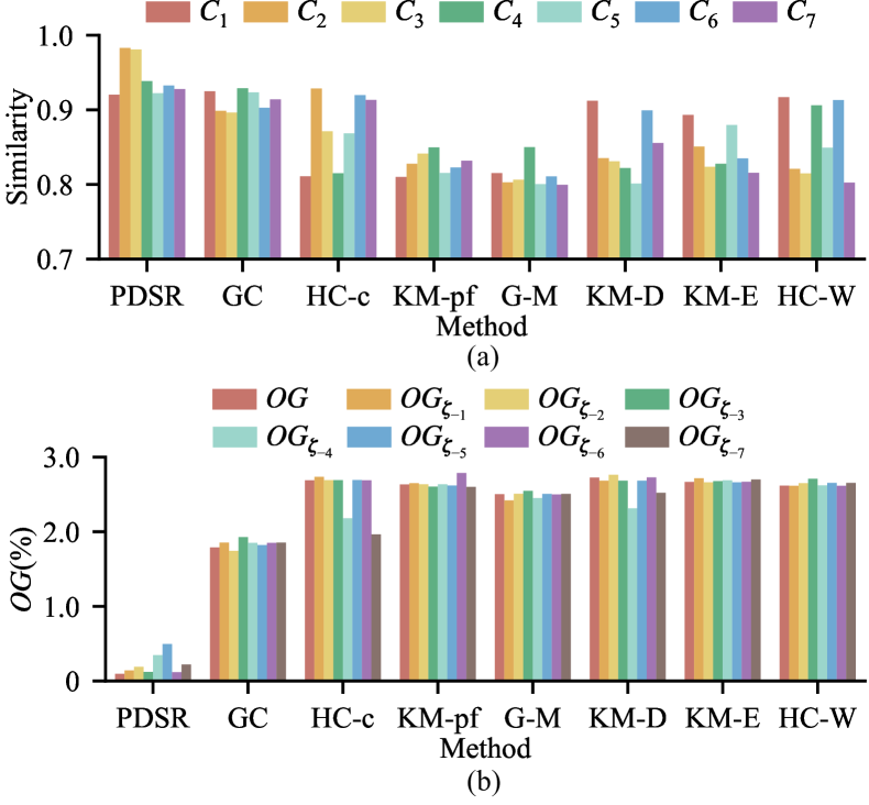
Figure 4: Comparative results for $N=400$ and $K=7$: (a) cluster decision similarity and (b) representative scenario effectiveness.

Computational Efficiency: The Benchmark struggles with computational complexity when $N$ is large. For example, for $N=400$ and $N=500$, the Benchmark takes nearly 38 and 60 mins, respectively. Moreover, for $N\geq 600$, computing times become impractical for the Benchmark. The DDSR methods, however, overcome computation bottlenecks, but at the price of potentially large $OG(\%)$ values. GC and PDSR decompose the original SBSO problem into mostly parallelizable and simple scenario-specific subproblems. Specifically, both GC and PDSR involve $N$ parallel computations followed by $N(N-1)$ parallel computations to determine matrix $\bm{F}$. In this paper, the computation time for each scenario-specific subproblem is $\tau_{\text{p}}<0.3s$ (with LinDistFlow model). Theoretically, with $N(N-1)$ parallel processes available, the computation time for calculating the $\bm{F}$ matrix can be reduced to $2\times\tau_{\text{p}}=0.6$s . For $N=400$ and $K=7$, after calculating the $\bm{F}$ matrix, the MILP clustering problem is solved consistently with MIP-gap with $\tau_{\text{c}}<3$s. We define $\tau_{\text{o}}(K)$ as the time required to solve (2) with $K$ representative scenarios and $\tau_{\text{o}}(7)<3s$. Generally, with $W$ parallel processors, the total computation time of the PDSR is

$$\tau:=(\lceil N/W\rceil+\lceil{N(N-1)/W\rceil)\tau_{\text{p}}+\tau_{\text{c}}+\tau_{\text{o}}(K)}.$$

For example, with $N=400$ and a practical $W=100$ processors, $\tau=8$ mins (or 21% of the Benchmark). Furthermore, as long as the original set of scenarios and SBSO problem formulation remain unchanged, matrix $\bm{F}$ can be stored and re-used. In conclusion, the PDSR framework can effectively reduce computational complexity while achieving a low SR optimality gap.

Scalability: We further compare the $OG(\%)$ results under different $N$ and $K$, as illustrated in Fig. 5. In Figs. 5(a,b), we observe that the proposed PDSR framework outperforms DDSR methods and GC across all values of $N$ and $K$, as evidenced by its consistently lower $OG(\%)$. This underscores the distinct superiority of the PDSR framework in identifying salient scenarios. Interestingly, the PDSR results (in blue) with $N=100$ has smaller $OG(\%)$ than the DDSR methods even for $N=400$, which means that to attain a comparable level of OG, the PDSR framework requires far fewer scenarios. Besides, As expected, increasing $K$ decreases the $OG(\%)$ for PDSR. However, for DDSR methods and GC, this inherent structural benefit of PSDR is not present. Furthermore, we conduct the performance comparison with a large original scenario set, using $N=1000$ and $K=10$ (i.e., a 99% reduction) as an example in Fig. 5(c). In this case, the original SBSO problem in (1) is computationally intractable. Therefore, we use $F(z^{\ast}_{\bm{\zeta}},\bm{\xi})$ as the performance evaluation metric, instead of $OG(\%)$. A smaller value of $F(z^{\ast}_{\bm{\zeta}},\bm{\xi})$ indicates a better approximation to the original SBSO optimality. Notably, PDSR outperforms other SR methods with the lowest $F(z^{\ast}_{\bm{\zeta}},\bm{\xi})$. Based on the representative scenarios from PDSR, the day-ahead SBSO problem obtains superior operational strategies with high adaptability and effectiveness across different scenarios. Moreover, for $N=1000$ and $K=10$, we have $\tau_{\mathrm{c}}=50$s, indicating that the MILP formulation can be solved efficiently. In conclusion, the above comparative analysis further emphasizes the benefit of the proposed PDSR framework.

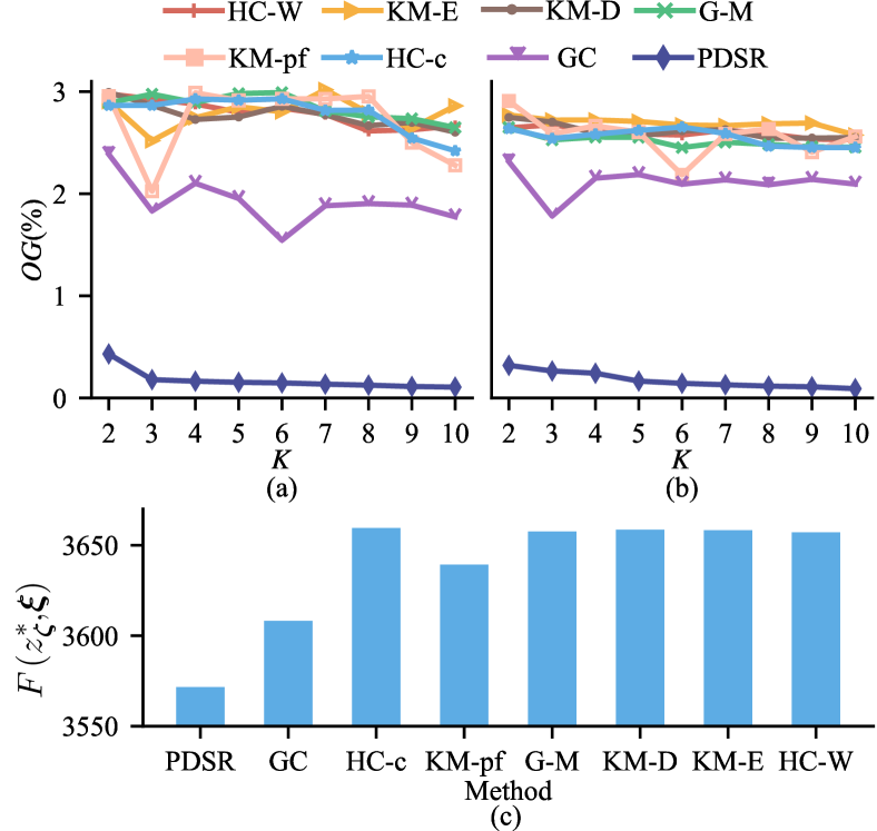
Figure 5: Comparing results for different $N$ and $K$: (a) $N=100$, (b) $N=400$ and (c) $N=1000$ and $K=10$.

IV-D Summarizing Discussion on PDSR Framework

For SBSO problems, the definition of “representativeness” is essential to construct the representative scenario set and yield effective strategies. In this paper, we demonstrate, both through theoretical analysis and numerical validation, that the “representativeness” should be defined as the decision applicability of the representative scenario to its represented scenario cluster. The advantages of the proposed PDSR framework lie in the following aspects:

1. Representativeness: With the problem space constructed from decision applicability, the PDSR framework successfully achieves a low optimality gap, demonstrating a significant level of representativeness.

2. Efficiency: The PDSR framework successfully captures the scenarios with significant impacts on the problem, especially the worst-case scenarios, enhancing the robustness and reliability. Moreover, in comparison to other SR methods, the PDSR framework effectively reduces the number of required scenarios with the same level of optimality gap, which is beneficial in cases with limited monitoring and data accumulation.

3. Determinateness: Instead of using heuristic methods, the PDSR framework transforms the processes of scenarios partitioning and representative scenarios selection into a MILP formulation, which attains deterministic and optimal outcomes with commercial solvers.

4. Generality: The proposed PDSR framework operates without reliance on probability distribution, and only have limited assumptions on the SBSO problem structure. As a result, the PDSR framework can be applied to a broad range of SBSO problems, ensuring high generality and scalability.

V Conclusion

In this paper, a novel problem-driven scenario reduction (PDSR) framework is proposed for power system SBSO problems, which fully incorporates the problem structure into the SR process. Specifically, we utilize the mutual decision applicability to construct the problem space as the input for SR, and propose the problem-driven distance metric to measure the similarity of scenarios in problem space. That is, PDSR decomposes the original large-scale and complex optimization problem into independent and simpler scenario-specific subproblems, thus, significantly decreasing computational complexity. Thus, the presented PDSR framework obtains near-optimal approximation accuracy with just a few salient representative scenarios whithin acceptable computation time, as illustrated with an extensive case study that balances operational energy storage capacity and economic costs. Moreover, a comprehensive comparative analysis with other SR methods is provided for different $N$ and $K$ values and demonstrates broadly the superior performance of our PDSR framework.

Future work will focus on further scaling Algorithm 1 by filtering the original scenario set for PDSR to reduce the size of the $\bm{F}$ matrix necessary to guarantee the desired optimality gap. Additionally, PDSR will benefit from extending the analysis to characterize the impacts of local solutions arising from non-convex problems, such as with the AC optimal power flow. Lastly, we are interested in extending the PDSR framework to other SBSO problems relevant to power engineering.

-A Proof of Proposition 1

In this part, we prove that the proposed problem-driven distance metric in (10) satisfies the required properties of (7).

Proof.

C1) Consistency: First we notice that $\zeta_{k}=\xi_{i}\Rightarrow d(\zeta_{k},\xi_{i})=0$. Conversely, given that both $c(\zeta_{k},\xi_{i}),\ c(\xi_{i},\zeta_{k})$ are nonnegative, $d(\zeta_{k},\xi_{i})=0$ implies $c(\zeta_{k},\xi_{i})=c(\xi_{i},\zeta_{k})=0$, thus $z_{\zeta_{k}}^{\ast}=z_{\xi_{i}}^{\ast}$. We reasonably require the problem to satisfy the assumption that $z_{\zeta_{k}}^{\ast}=z_{\xi_{i}}^{\ast}\Rightarrow\zeta_{k}=\xi_{i}$. This hypothesis rests on the premise that $F(z,\xi)$ is highly sensitive to variations in $\xi$ at particular $z$, suggesting that identical solutions imply identical scenarios. This assumption depends on the problem structure and can be restrictive. For certain problems dissatisfy this assumption, we can adjust the PDD by simply incorporating a regularized scaled norm component ($\mu>0$) as

$$\begin{split}\tilde{d}(\xi_{i},\zeta_{k})&=F(z_{\zeta_{k}}^{\ast},\xi_{i})-F(z_{\xi_{i}}^{\ast},\xi_{i})\\ &\quad+F(z_{\xi_{i}}^{\ast},\zeta_{k})-F(z_{\zeta_{k}}^{\ast},\zeta_{k})+\mu\|\zeta_{k}-\xi_{i}\|_{2}.\end{split}$$ (25)

In this case, $\tilde{d}(\xi_{i},\zeta_{k})=0\Rightarrow\zeta_{k}=\xi_{i}$ holds for any $\mu$. In this paper, we set $\mu=0$ and continue to use $d(\zeta_{k},\xi_{i})$ for brevity, but all the proofs and algorithms can be adapted for $\tilde{d}(\xi_{i},\zeta_{k})$.

C2) Symmetricity: From definition, $d(\zeta_{k},\xi_{i})=d(\xi_{i},\zeta_{k})$.

C3) Convergence: As $\delta\rightarrow 0$, $\zeta_{k}$ and $\xi_{i}$ become arbitrarily close. Given the Lipschitz continuity of $F(z,\xi)$ with respect to $\xi$, it follows that $F(z_{\zeta_{k}}^{\ast},\xi_{i})\rightarrow F(z_{\zeta_{k}}^{\ast},\zeta_{k})$ and $F(z_{\xi_{i}}^{\ast},\xi_{i})\rightarrow F(z_{\xi_{i}}^{\ast},\zeta_{k})$. Consequently, $d(\zeta_{k},\xi_{i})$ tends to 0.

C4) Triangle inequality: Let $\lambda(\xi_{i})=2\sup_{z\in Z}|F(z,\xi_{i})|$, given $F(z,\xi)$ is bounded for all $z$ and $\xi$. We have $F(z_{\zeta_{k}}^{\ast},\xi_{i})-F(z_{\xi_{i}}^{\ast},\xi_{i})<|F(z_{\zeta_{k}}^{\ast},\xi_{i})|+|F(z_{\xi_{i}}^{\ast},\xi_{i})|<\lambda(\xi_{i})$, and similar for $\lambda(\zeta_{k})$. Thus, we have $d(\zeta_{k},\xi_{i})<\lambda(\zeta_{k})+\lambda(\xi_{i})$. ∎

References

- [1] L. A. Roald, D. Pozo, A. Papavasiliou et al., “Power systems optimization under uncertainty: A review of methods and applications,” Electric Power Systems Research, vol. 214, p. 108725, 2023.
- [2] Y. Guo, K. Baker, E. Dall’Anese et al., “Data-based distributionally robust stochastic optimal power flow—part i: Methodologies,” IEEE Trans. on Power Systems, vol. 34, no. 2, pp. 1483–1492, 2018.
- [3] Y. Qiu, Q. Li, Y. Ai et al., “Two-stage distributionally robust optimization-based coordinated scheduling of integrated energy system with electricity-hydrogen hybrid energy storage,” Prot. Control Mod. Power Syst., vol. 8, no. 2, pp. 1–14, 2023.
- [4] Z. Guo, P. Pinson, S. Chen et al., “Chance-constrained peer-to-peer joint energy and reserve market considering renewable generation uncertainty,” IEEE Trans. on Smart Grid, vol. 12, no. 1, pp. 798–809, 2020.
- [5] N. Qi, P. Pinson, M. R. Almassalkhi et al., “Chance-constrained generic energy storage operations under decision-dependent uncertainty,” IEEE Trans. on Sustainable Energy, vol. 14, no. 4, pp. 2234–2248, 2023.
- [6] B. Zeng and L. Zhao, “Solving two-stage robust optimization problems using a column-and-constraint generation method,” Operations Research Letters, vol. 41, no. 5, pp. 457–461, 2013.
- [7] Y. Zhang, F. Liu, Z. Wang et al., “Robust scheduling of virtual power plant under exogenous and endogenous uncertainties,” IEEE Trans. on Power Systems, vol. 37, no. 2, pp. 1311–1325, 2021.
- [8] W. Yin, S. Feng, and Y. Hou, “Stochastic wind farm expansion planning with decision-dependent uncertainty under spatial smoothing effect,” IEEE Trans. on Power Systems, 2022.
- [9] Y. Liu, D. Liu, and H. Zhang, “Stochastic unit commitment with high-penetration offshore wind power generation in typhoon scenarios,” Journal of Modern Power Systems and Clean Energy, 2023.
- [10] N. Qi, L. Cheng, H. Li et al., “Portfolio optimization of generic energy storage-based virtual power plant under decision-dependent uncertainties,” Journal of Energy Storage, vol. 63, p. 107000, 2023.
- [11] L. Liu, X. Hu, J. Chen et al., “Embedded scenario clustering for wind and photovoltaic power, and load based on multi-head self-attention,” Prot. Control Mod. Power Syst., vol. 9, no. 1, pp. 122–132, 2024.
- [12] N. Huang, W. Wang, S. Wang et al., “Incorporating load fluctuation in feature importance profile clustering for day-ahead aggregated residential load forecasting,” IEEE Access, vol. 8, pp. 25 198–25 209, 2020.
- [13] D. Z. Fitiwi, F. de Cuadra, L. Olmos et al., “A new approach of clustering operational states for power network expansion planning problems dealing with res (renewable energy source) generation operational variability and uncertainty,” Energy, vol. 90, pp. 1360–1376, 2015.
- [14] M. Sun, F. Teng, X. Zhang et al., “Data-driven representative day selection for investment decisions: A cost-oriented approach,” IEEE Trans. on Power Systems, vol. 34, no. 4, pp. 2925–2936, 2019.
- [15] J. Xu, B. Wang, Y. Sun et al., “A day-ahead economic dispatch method considering extreme scenarios based on wind power uncertainty,” CSEE Journal of Power and Energy Systems, vol. 5, no. 2, pp. 224–233, 2019.
- [16] X. Liu, M. Shahidehpour, Z. Li et al., “Microgrids for enhancing the power grid resilience in extreme conditions,” IEEE Trans. on Smart Grid, vol. 8, no. 2, pp. 589–597, 2017.
- [17] X. Dong, Y. Sun, S. M. Malik et al., “Scenario reduction network based on wasserstein distance with regularization,” IEEE Trans. on Power Systems, vol. 39, no. 1, pp. 4–13, 2024.
- [18] T. Teeraratkul, D. O’Neill, and S. Lall, “Shape-based approach to household electric load curve clustering and prediction,” IEEE Trans. on Smart Grid, vol. 9, no. 5, pp. 5196–5206, 2018.
- [19] Y. Liu, R. Sioshansi, and A. J. Conejo, “Hierarchical clustering to find representative operating periods for capacity-expansion modeling,” IEEE Trans. on Power Systems, vol. 33, no. 3, pp. 3029–3039, 2017.
- [20] S. Lin, C. Liu, Y. Shen et al., “Stochastic planning of integrated energy system via frank-copula function and scenario reduction,” IEEE Trans. on Smart Grid, vol. 13, no. 1, pp. 202–212, 2021.
- [21] Z. Shi, L. Wu, and Y. Zhou, “Predicting household energy consumption in an aging society,” Applied Energy, vol. 352, p. 121899, 2023.
- [22] H. Teichgraeber and A. R. Brandt, “Clustering methods to find representative periods for the optimization of energy systems: An initial framework and comparison,” Applied Energy, vol. 239, pp. 1283–1293, 2019.
- [23] D. Bertsimas and N. Mundru, “Optimization-based scenario reduction for data-driven two-stage stochastic optimization,” Operations Research, vol. 71, no. 4, pp. 1343–1361, 2022.
- [24] M. Hewitt, J. Ortmann, and W. Rei, “Decision-based scenario clustering for decision-making under uncertainty,” Annals of Operations Research, vol. 315, no. 2, pp. 747–771, 2022.
- [25] J. Keutchayan, J. Ortmann, and W. Rei, “Problem-driven scenario clustering in stochastic optimization,” Computational Management Science, vol. 20, no. 1, p. 13, 2023.
- [26] J. Dupačová, N. Gröwe-Kuska, and W. Römisch, “Scenario reduction in stochastic programming,” Mathematical Programming, vol. 95, no. 3, pp. 493–511, 2003.
- [27] M. Almassalkhi, S. Brahma, N. Nazir et al., “Hierarchical, grid-aware, and economically optimal coordination of distributed energy resources in realistic distribution systems,” Energies, vol. 13, no. 23, 2020.
- [28] M. Baran and F. Wu, “Optimal sizing of capacitors placed on a radial distribution system,” IEEE Trans. on Power Delivery, vol. 4, no. 1, pp. 735–743, 1989.
- [29] Original scenarios. [Online]. Available: https://github.com/Yingrui-Z/Original-Scenarios