Localized Distributional Robustness in Submodular Multi-Task Subset Selection

Abstract

In this work, we approach the problem of multi-task submodular optimization with the perspective of local distributional robustness, within the neighborhood of a reference distribution which assigns an importance score to each task. We initially propose to introduce a regularization term which makes use of the relative entropy to the standard multi-task objective. We then demonstrate through duality that this novel formulation itself is equivalent to the maximization of a submodular function, which may be efficiently carried out through standard greedy selection methods. This approach bridges the existing gap in the optimization of performance-robustness trade-offs in multi-task subset selection. To numerically validate our theoretical results, we test the proposed method in two different setting, one involving the selection of satellites in low Earth orbit constellations in the context of a sensor selection problem, and the other involving an image summarization task using neural networks. Our method is compared with two other algorithms focused on optimizing the performance of the worst-case task, and on directly optimizing the performance on the reference distribution itself. We conclude that our novel formulation produces a solution that is locally distributional robust, and computationally inexpensive.

Keywords: Optimization, robustness, submodularity.

1 Introduction

Submodular functions have for long been the focus of extensive studies[1, 2, 3, 4], thanks to their propensity to occur naturally in many distinct domains such as economics and algorithmic game theory [5, 6, 7] and machine learning[8, 9, 10, 11, 12, 13, 14, 15, 16, 17], within many distinct problems, ranging from sensor selection [18, 4, 19, 20] to social network modeling [21]. In simplest terms, a submodular function is a set function that possesses the diminishing marginal gains property [22]. This property, at first glance, enables one to draw an analogy between submodular functions and concave functions in the continuous domain. However, interestingly, a similar analogy may be drawn between submodular functions and convex functions in the continuous domain, as well, through the use of certain extensions of submodular functions onto the continuous domain [23, 4]. The similarity of submodular functions to both convex and concave functions, the white whales of optimization literature, has also garnered interest in the study of the optimization of submodular functions.

The quintessential submodular optimization problem is that of the maximization of a submodular function under a cardinality constraint. This problem entails selecting a subset out of a ground set $N$ of elements, such that the size of the selection does not exceed a preset constraint value, and the evaluation of the selection under the submodular function is as high as possible. The evaluation $f(S)$ of a subset $S\subseteq N$ by $f$ is commonly called the score or utility of the set $S$. The following formulation, where, $f$ is a submodular function, $N$ is the ground set and $K$ is a positive integer representing the cardinality constraint, expresses this problem in mathematical terms[5]:

$$\begin{split}&\max_{S\subseteq N}f(S)\\ &\text{s. t. }\lvert S\rvert\leq K.\end{split}$$ (1)

The notion of robustness occurs very frequently in optimization literature and is the object of much consideration. Although there are differing definitions of robustness depending on the context at hand, such as being immune to removals from the solution [24], or to slight changes in parameters or input data[25], and others[26], it always encompasses the general idea of a produced solution to a problem (the output) staying correct and valid under perturbations to the input. In the present context of submodular optimization, one conception of robustness that is commonly encountered is multi-task robustness. As the name implies, with this conception, the aim is to algorithmically produce a solution set whose utility with respect to multiple submodular functions $f^{1},\ldots,f^{n}$ is satisfactory.

As it stands, the notion of being “satisfactory” is intentionally left to be vague, and the problem can be formulated in multiple ways to fit the description. A straightforward interpretation with this goal in mind might lead to what we will call the worst-case formulation [4, 27, 28, 29], which aims to focus on producing a solution that maximizes the worst-performing objective function among all. Using the shorthand notation $[n]\vcentcolon=\{1,\ldots,n\}$, this formulation is as follows:

$$\begin{split}&\max_{S\subseteq N}\min_{i\in[n]}f^{i}(S)\\ &\text{s. t. }\lvert S\rvert\leq K.\end{split}$$ (2)

A shortcoming of this formulation is the fact that it can be viewed as being too pessimistic[30], dedicating all resources to the maximization of the worst-performing objective function, at the expense of disregarding the others. In scenarios where one objective function is a clear outlier, as in it always scores significantly lower than all others, this approach may effectively lead to getting low utility on all functions in pursuit of the hopeless aim of maximizing that outlier.

Another way to formulate the multi-task robust problem could be to adopt what we will call the average-case formulation [30, 31], which aims to directly optimize the arithmetic average of all the objective functions. In this case, the formulation would be

$$\begin{split}&\max_{S\subseteq N}\frac{1}{n}\sum_{i=1}^{n}f^{i}(S)\\ &\text{s. t. }\lvert S\rvert\leq K.\end{split}$$ (3)

The apparent shortcoming of this formulation is the fact that contrary to the previous formulation, it provides no guarantees whatsoever about how low the utility with respect to any individual objective function may be. In essence, one or multiple objective functions could be scoring arbitrarily badly, as long as the other objective functions are scoring well enough to compensate for the underperformers.

The previous two formulations, even with their stated shortcomings, may very well be acceptable approaches, especially in the absence of any additional information. However, we argue that if we possess additional information on the nature of the objective functions, or a system at hand, for whose various tasks we use the multiple objective functions to model, we can progress to a more meaningful formulation. Suppose, for instance, that we have access to a reference distribution, an $n-$dimensional discrete probability distribution $Q\in\Delta_{n}$. In a practical setting, the reference distribution $Q$ may be obtained by a decision-maker subjectively assigning importance scores to each objective function, or by a frequentist approach, where the value assigned to each function would be given by how frequently the task that is modeled by said function is performed by the system. It is reasonable to argue that the reference distribution can facilitate incorporating the intent and priority of the main stakeholders in the problem. The incorporation of this additional information to the previous formulation leads to a generalization of Problem (3), where the reference distribution is simply assumed to be uniform. This idea is encapsulated in the following formulation:

$$\begin{split}&\max_{S\subseteq N}\sum_{i=1}^{n}Q_{i}f^{i}(S)\\ &\text{s. t. }\lvert S\rvert\leq K.\end{split}$$ (4)

We note that this previous formulation reduces exactly to Problem (2) when $P^{*}$ is a one-hot discrete distribution, indicating the worst-performing objective function.

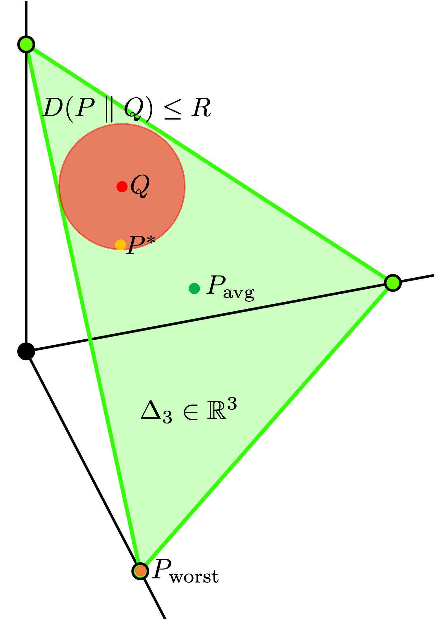
Fig. 1: Illustration of the three discrete distributions on the $3-$dimensional simplex that the three discussed approaches optimize. $P_{\text{worst}}$ corresponds to the global worst-case task scenario, assigning a weight of $1$ to the worst-case task and a weight of $0$ to all the others, residing on a vertex of the simplex. $P_{\text{avg}}$ assigns uniform weight to all tasks, and lies in the center of the simplex. $Q$ is the reference distribution within a neighborhood of which we want to achieve local robustness. $P^{\ast}$ is the local worst-case distribution within that neighborhood of $Q$.

1.1 Contribution

Based on this previous formulation, we present our novel robust formulation, which not only makes use of the reference distribution to simply weigh each objective function but to act as the center of a neighborhood of robustness, within which we will aim to be robust. The initial candidate formulation for this is as follows:

$$\begin{split}&\max_{S\subseteq N}\min_{P\in\Delta_{n}}\sum^{n}_{i=1}P_{i}f^{i}(S)\\ &\text{s. t. }\lvert S\rvert\leq K,\;D(P\;\|\;Q)\leq R,\end{split}$$ (5)

where the constraint $D(P\;\|\;Q)\leq R$ designates the requirement that we localize ourselves to a specified neighborhood of robustness, with radius $R$, only within which we will maximize our objectives, weighed by the worst possible distribution. $D(P\;\|\;Q)$ is intentionally unspecified and could be any metric or divergence. For an investigation of different statistical distances for $D(P\;\|\;Q)$, we refer the reader to Section 3.

Before we proceed with the theoretical analysis of Problem 5, we propose one last change to the formulation to make it more tractable. We relax the formulation by introducing the constraint $D(P\;\|\;Q)\leq R$ into the objective via a penalizing regularization constant $\lambda\geq 0$, instead of strictly enforcing it. This change reflects the standard idea of introducing Lagrange multipliers, utilized frequently in continuous optimization[32]. With this final addition, our novel formulation becomes

$$\begin{split}&\max_{S\subseteq N}\min_{P\in\Delta_{n}}\sum^{n}_{i=1}P_{i}f^{i}(S)+\lambda D(P\;\|\;Q)\\ &\text{s. t. }\lvert S\rvert\leq K.\end{split}$$ (6)

1.2 Related Works and Significance

Robust submodular optimization. Reference [18] is a fundamental work in establishing the notion of robustness in submodular optimization that is adopted in the current manuscript, and proposing an algorithmic solution to the worst-case formulation of Problem (2), namely, the Submodular Saturation Algorithm (SSA). This algorithm will be discussed considerably in the following sections and will constitute one of the baselines for our work to be compared against. References [33, 29] similarly adopt the same formulation of Problem (2) in consideration of robustness. The former of these works generalizes the results of [18], which deals with the cardinality-constrained problem, to cases where knapsack or other matroid constraints are present, including the case where the constraints themselves are submodular, as well. The latter shifts the focus to achieving higher computational efficiency, aiming for a fast and practical algorithm with asymptotic approximation guarantees when $n$, the number of objective functions is increased arbitrarily. Reference [30] proposes a novel notion of robustness that yet pertains to the context of multiple objective functions. The authors firstly motivate their novel approach by drawing attention to the pessimistic nature of Problem (2). They instead propose an approach that entails the maximization of the $p$^th quantile of the objective functions, where $0\leq p<1$. To simplify, this approach may be viewed as forgoing the consideration of the worst-performing $p$^th of the objective functions in favor of maximizing the remaining. Different from all of the previously mentioned works, the present work shifts the focus to the scope of distributional robustness, focusing on localizing our goal of robustness within a subset of the $n-$dimensional simplex, in a neighborhood of a reference distribution. References [24, 34] adopt one of the aforementioned different notions of robustness within the context of submodular optimization. In these works, the notion of robustness is against the post-processing of solutions for the arbitrary or adversarial deletion of a certain number of elements, rather than robustness against multiple submodular objective functions.

Distributionally-robust optimization. Our work is closely related to and motivated by the distributionally robust optimization paradigm. In a very general sense, distributionally robust optimization is a paradigm where some uncertainty about the nature of the problem is governed by a probability distribution and the goal is to leverage the information we have about this governing distribution with the goal of optimization or optimal decision-making. Reference [35] approaches a convex optimization problem in the context of distributionally robust optimization. Reference [36] broadens the scope of consideration of online optimization of nonconvex functions. In particular, the authors use relative entropy regularization, which we also employ in this work. Reference [31], much like our work, deals with distributionally-robust optimization of submodular functions. The authors here work in the presence of stochastic submodular objective functions that are drawn from a given reference distribution and aim to maximize the expected value of such functions. They propose an approach that entails a variance-regularized objective, making use of the multilinear extension of submodular functions and the Momentum Frank-Wolfe algorithm. In contrast to this line of work, we leverage distributionally robust optimization for discrete multi-task subset selection and demonstrate the possibility of formulating the distributionally robust problem as a simple submodular maximization problem, essentially allowing us to produce a distributionally robust solution at no additional cost to produce a solution to the naive formulation of Problem (4).

2 Preliminaries and Background

We begin by introducing the concept of the marginal gain in set functions because it is key in defining submodular functions.

Definition 1 (Marginal gain).

Given a set function $f\vcentcolon 2^{N}\rightarrow\mathbb{R}$ and $A,B\subseteq N$, we denote $f(B\cup A)-f(B)$, the marginal gain in $f$ due to adding $A$ to $B$, by $\Delta_{f}(A|B)$.
When the set $A$ is a singleton, i.e., $A=\{a\}$, we drop the curly brackets to adopt the short-hand notation $\Delta_{f}(a|B)$.

Now, we introduce the notion of submodularity using this definition.

Definition 2 (Submodularity).

A set function $f\vcentcolon 2^{N}\rightarrow\mathbb{R}$ is submodular if for every $A\subseteq B\subseteq N$ and $e\in N\setminus B,$ it holds that

$$\Delta_{f}(e|A)\geq\Delta_{f}(e|B).$$ (7)

This definition of submodularity highlights the renowned diminishing marginal gains property of submodular functions, which is commonly referred to when making the analogy to discrete concave functions. However, the following equivalent definition, although less intuitive, proves to be more useful in certain situations, including a part of our analysis:

Definition 3 (Submodularity, alternative).

A set function $f\vcentcolon 2^{N}\rightarrow\mathbb{R}$ is submodular if for every $A,B\subseteq N,$

$$f(A\cap B)+f(A\cup B)\leq f(A)+f(B).$$ (8)

The common notion in thinking about a submodular function $f$ is that it scores each set by its utility, as such, we will commonly refer to the evaluation $f(S)$ as the utility, performance, or score of set $S$.

Finally, we introduce two additional useful properties of set functions, that are combined with submodularity in the derivation of theoretical guarantees for approximation algorithms that optimize submodular functions.

Definition 4 (Normalized set functions).

A set function $f\vcentcolon 2^{N}\rightarrow\mathbb{R}$ is normalized if $f(\emptyset)=0$.

Definition 5 (Monotone nondecreasing set functions).

A set function $f\vcentcolon 2^{N}\rightarrow\mathbb{R}$ is monotone nondecreasing if for every $A\subseteq B\subseteq N,$ we have $f(A)\leq f(B).$

Note that a set function $f$ having both of the last two properties ensures that $f\geq 0$.

Possibly the most fundamental result in submodular optimization concerns the maximization of normalized, monotone nondecreasing submodular functions under a cardinality constraint. In this case, the iterative Greedy algorithm, which simply consists of going over the entire set of remaining elements at each iteration and adding the one with the highest marginal gain to the solution, obtains an approximation ratio of $1-1/e$. Although simple in principle, Greedy is demonstrably the optimal approximation algorithm, unless $\text{P}=\text{NP}$.[22]

While Greedy is demonstrably optimal and very easy to implement, its standard form is usually avoided due to the computational cost of reevaluating every remaining element at each iteration that it incurs. Several methods have been proposed to circumvent this shortcoming, two significant ones being Lazy Greedy[37], and Stochastic Greedy[38]. In particular, Stochastic Greedy achieves a reduced computational cost by reducing its evaluations to a subset of the remaining elements sampled uniformly at random at each iteration, instead of reevaluating every element. Stochastic Greedy also enjoys, on expectation, an approximation ratio similar to that of Greedy, with an additional term that designates the dependence on the cardinality of the randomly sampled subset.

Theorem 1 (Stochastic Greedy approximation ratio).

[38] Let $f\vcentcolon 2^{N}\rightarrow\mathbb{R}$ be a normalized, monotone nondecreasing submodular function. Let $R=(\lvert N\rvert/K)\log(1/\epsilon)$ be the size of the sampled set at each iteration of Stochastic Greedy used in the solution of Problem (1), where $\epsilon\in(0,1)$. Then, on expectation, Stochastic Greedy achieves an approximation ratio of $1-1/e-\epsilon$, i.e., Stochastic Greedy produces a solution $\hat{S}$ which satisfies

$$\mathbb{E}[f(\hat{S})]\geq(1-1/e-\epsilon)f(S^{\ast}),$$ (9)

where $S^{\ast}$ is a maximizer of Problem (1).

3 Investigation of Various Statistical Distances for Regularization

In the formulation of Problem (6), we have intentionally left unspecified the statistical distance $D(P\;\|\;Q)$ to be used in the regularization term, in order to localize our region of interest to a neighborhood around the reference distribution $Q$. In this section, we will be specifically interested in investigating which choices of $D(\cdot\;\|\;\cdot)$ lead to favorable algorithmic solutions and theoretical guarantees for Problem (6). In particular, of specific interest will be such $D(\cdot\;\|\;\cdot)$ that preserve the submodular nature of the problem. For, ensuring that the problem remains submodular allows us to produce a locally robust solution essentially at no additional cost with respect to the non-robust formulation of Problem (1), by falling back to our familiar tools such as Stochastic Greedy, and enjoying theoretical guarantees such as that presented in Theorem 1.

We first shift our attention to metrics induced by $\ell^{p}$ norms. One choice for $D(P\;\|\;Q)$ that leads to a favorable algorithmic solution is the metric induced by the $\ell^{\infty}$ norm, i.e., $D(P\;\|\;Q)=\lVert P-Q\rVert_{\infty}\vcentcolon=\max_{i\in[n]}\lvert P_{i}-Q_{i}\rvert.$ With this selection, Problem (6) becomes

$$\begin{split}&\max_{S\subseteq N}\min_{P\in\Delta_{n}}\sum^{n}_{i=1}P_{i}f^{i}(S)+\lambda\lVert P-Q\rVert_{\infty}\\ &\text{s. t. }\lvert S\rvert\leq K.\end{split}$$ (10)

In this case, we may exploit the reduction of the inner problem of (10) to a linear program to derive a result. Indeed, since we know that the optimal point of a linear program will occur at one of the vertices of the feasible region [39], we have the following equivalence:

$$\begin{split}\min_{P\in\Delta_{n}}\sum^{n}_{i=1}P_{i}f^{i}(S)+\lambda\lVert P-Q\rVert_{\infty}\equiv\min_{i\in[n]}f^{i}(S)-\lambda Q_{i}.\end{split}$$ (11)

Hence, Problem (10) reduces, in whole, to

$$\begin{split}&\max_{S\subseteq N}\min_{i\in[n]}f^{i}(S)-\lambda Q_{i}\\ &\text{s. t. }\lvert S\rvert\leq K.\end{split}$$ (12)

The main observation about Problem (12) is that it is strikingly similar to the worst-case formulation of Problem (2), however, in addition, the information due to the reference distribution $Q$ still holds influence. We propose to use SSA [18] with a slight modification enabling the incorporation of the reference distribution $Q$ for the solution of Problem (12). The full algorithm, which we name Saturate with Preference, is presented in Algorithm 1.

It is worth noting that the choice of the metric induced by the $\ell^{1}$ norm, i.e., $D(P\;\|\;Q)=\lVert P-Q\rVert_{1}\vcentcolon=\sum_{i=1}^{n}\lvert P_{i}-Q_{i}\rvert$, through the same reduction of the inner problem to a linear program, and the same equivalence of (11), results in the same formulation of Problem (12). Since $P$ and $Q$ are discrete probability distributions, one may also view the quantity $\lVert P-Q\rVert_{1}$ as a scaled version of the total variation distance, an example of an $f-$divergence, which motivates the discussion of the next section, in using one $f-$divergence with particularly significant theoretical outcomes, namely, the relative entropy or KL-divergence.

Algorithm 1 Saturate with Preference

Input: Finite collection of monotone nondecreasing submodular functions $f^{1},\ldots f^{n}$, ground set $N$, cardinality constraint $K\in\mathbb{N}$, regularization parameter $\lambda\geq 0$, reference distribution $Q\in\Delta_{n}$
   Output: Solution set $S$

1:$k_{m}\leftarrow 0$

2:$k_{M}\leftarrow\min_{i}f^{i}(N)-\lambda Q_{i}$

3:$\S\leftarrow\emptyset$

4:while $k_{M}-k_{m}\geq 1/n$ do

5:   $k\leftarrow(k_{M}-k_{m})/2$

6:   Define $\bar{f}_{(k)}(\mathord{\cdot})\leftarrow\frac{1}{n}\sum_{i=1}^{n}\min\{f^{i}(\mathord{\cdot})-\lambda Q_{i},k\}$

7:   $\hat{S}\leftarrow\textsc{Greedy}(\bar{f}_{(k)},k)$

8:   if $\lvert\hat{S}\rvert>\alpha K$ then

9:      $k_{M}\leftarrow k$

10:   else

11:      $k_{m}\leftarrow k$

12:      $S\leftarrow\hat{S}$

13:   end if

14:end while

4 Relative Entropy Regularization

The choice of relative entropy for the regularizing function, i.e., $D(P\;\|\;Q)=D_{\text{KL}}(P\;\|\;Q)$, where

$$D_{\text{KL}}(P\;\|\;Q)\vcentcolon=\sum_{i=1}^{n}P_{i}\log\left(\frac{P_{i}}{Q_{i}}\right),$$ (13)

leads to the most significant theoretical outcomes, as will be seen in the following analysis. With this choice, the novel formulation is as follows:

$$\begin{split}&\max_{S}\min_{P}\sum^{n}_{i=1}P_{i}f^{i}(S)+\lambda D_{\text{KL}}(P\;\|\;Q)\\ &\text{s. t. }S\subseteq N,|S|\leq K\text{, and }P\in\Delta_{n}.\end{split}$$ (14)

We start our analysis of the novel formulation by considering the dual formulation of the inner minimization problem in (14), by introducing a Lagrange multiplier for the constraint $P\in\Delta_{n}$ in Problem (14). We first note that this constraint is equivalent to the two constraints (i) $P_{i}\geq 0$ for all $i\in[n]$ and (ii) $\sum_{i=1}^{n}P_{i}=1.$ Introducing a Lagrange multiplier only for constraint (ii), we write the Lagrangian of the inner problem as

$$\mathcal{L}\left(P,S,\mu\right)=\sum_{i=1}^{n}P_{i}f^{i}(S)+\lambda D_{\text{KL}}(P\;\|\;Q)+\mu\sum_{i=1}^{n}P_{i}-\mu.$$ (15)

Minimizing $\mathcal{L}(P,S,\mu)$ over $P$ will yield the dual formulation of the inner problem of (14). We solve

$$\begin{split}&\min_{P}\mathcal{L}\left(P,S,\mu\right)\\ &\text{s. t. }P_{i}\geq 0\text{ for all }i\in[n].\end{split}$$ (16)

Leveraging the convexity of the problem in $P$, we simply look at the partial derivative of $\mathcal{L}$ with respect to each $P_{i},$ which is given by

$$\frac{\partial\mathcal{L}}{\partial P_{i}}=f^{i}(S)+\lambda\log\left(\frac{P_{i}}{Q_{i}}\right)+\lambda+\mu.$$ (17)

Setting this quantity equal to $0$, we obtain the minimizer $P_{i}^{*}$:

$$P_{i}^{*}=Q_{i}\exp{\left(-\frac{\lambda+\mu+f^{i}(S)}{\lambda}\right)}.$$ (18)

Using this, along with the fact that $\sum_{i=1}^{n}P_{i}^{*}=1,$ we get

$$\begin{split}\sum_{i=1}^{n}P_{i}^{*}&=\sum_{i=1}^{n}Q_{i}\exp{\left(-\frac{\lambda+\mu+f^{i}(S)}{\lambda}\right)}\\ &=\sum_{i=1}^{n}Q_{i}\exp{\left(-\frac{f^{i}(S)}{\lambda}\right)}\exp{\left(-\frac{\lambda+\mu}{\lambda}\right)}=1.\end{split}$$ (19)

Then,

$$\lambda+\mu=\lambda\log\left(\sum_{i=1}^{n}Q_{i}\exp{\left(\frac{-f^{i}(S)}{\lambda}\right)}\right).$$ (20)

Now, evaluating $\mathcal{L}$ at the minimizer $P^{*}$, we obtain

$$\begin{split}\mathcal{L}(P^{*},S,\mu)&=\sum_{i=1}^{n}P_{i}^{*}f^{i}(S)+\lambda D_{\text{KL}}(P^{*}\;\|\;Q)\\ &=\sum_{i=1}^{n}Q_{i}\exp{\left(-\frac{\lambda+\mu+f^{i}(S)}{\lambda}\right)}f^{i}(S)\\ &+\lambda\sum_{i=1}^{n}Q_{i}\exp{\left(-\frac{\lambda+\mu+f^{i}(S)}{\lambda}\right)}\\ &\cdot\left[-\frac{\lambda+\mu+f^{i}(S)}{\lambda}\right]\\ &=-\left(\lambda+\mu\right)\sum_{i=1}^{n}Q_{i}\exp{\left(-\frac{\lambda+\mu+f^{i}(S)}{\lambda}\right)}.\\ \end{split}$$ (21)

Since we have

$$\begin{split}\sum_{i=1}^{n}Q_{i}\exp{\left(-\frac{\lambda+\mu+f^{i}(S)}{\lambda}\right)}=\sum_{i=1}^{n}P_{i}^{*}=1,\end{split}$$ (22)

(21) becomes

$$\begin{split}\mathcal{L}(P^{*},S,\mu)=-\left(\lambda+\mu\right).\end{split}$$ (23)

Finally, from (20), we obtain:

$$\begin{split}g(S)\vcentcolon=\mathcal{L}(P^{*},S,\mu)=-\lambda\log\left(\sum_{i=1}^{n}Q_{i}\exp{\left(\frac{-f^{i}(S)}{\lambda}\right)}\right).\end{split}$$ (24)

Hence, the dual formulation of Problem (14) becomes that of the maximization of another set function $g$:

$$\begin{split}&\max_{S\subseteq N}g(S)\\ &\text{s.t. }\lvert S\rvert\leq K.\end{split}$$ (25)

A simple analysis of the extreme cases of values for the regularization parameter $\lambda$ is revealing of the equivalence of the two problems. We evaluate the limit

$$\begin{split}\lim_{\lambda\to x}-\lambda\log\left(\sum_{i=1}^{n}Q_{i}\exp{\left(\frac{-f^{i}(S)}{\lambda}\right)}\right)=\\ \lim_{\lambda\to x}-\frac{\log\left(\sum_{i=1}^{n}Q_{i}\exp{\left(\frac{-f^{i}(S)}{\lambda}\right)}\right)}{\frac{1}{\lambda}}\end{split}$$ (26)

This limit is equivalent to

$$\lim_{\lambda\to x}\frac{\sum_{i=1}^{n}Q_{i}\exp{\left(\frac{-f^{i}(S)}{\lambda}\right)f^{i}(S)}}{\sum_{i=1}^{n}Q_{i}\exp{\left(\frac{-f^{i}(S)}{\lambda}\right)}}.$$ (27)

Letting $x\to\infty$, we have:

$$\begin{split}\lim_{\lambda\to\infty}\frac{\sum_{i=1}^{n}Q_{i}\exp{\left(\frac{-f^{i}(S)}{\lambda}\right)f^{i}(S)}}{\sum_{i=1}^{n}Q_{i}\exp{\left(\frac{-f^{i}(S)}{\lambda}\right)}}=\sum_{i=1}^{n}Q_{i}f^{i}(S).\end{split}$$ (28)

This is indeed the expected behavior, since letting $\lambda\to\infty$ in Problem (14) effectively assigns all importance to the regularization term, and necessarily forces one to have $P=Q$, making the objective

$$\begin{split}&\max_{S\subseteq N}\sum_{i=1}^{n}Q_{i}f^{i}(S)\\ &\text{s.t. }\lvert S\rvert\leq K,\end{split}$$ (29)

which is recovered exactly in (28).

On the other hand, letting $x=0$, the value of the limit is determined by the most dominant term in the sums in the numerator and the denominator, that is,

$$\begin{split}&\lim_{\lambda\to 0}\frac{\sum_{i=1}^{n}Q_{i}\exp{\left(\frac{-f^{i}(S)}{\lambda}\right)f^{i}(S)}}{\sum_{i=1}^{n}Q_{i}\exp{\left(\frac{-f^{i}(S)}{\lambda}\right)}}\\ &=\min_{i\in[n]}\frac{Q_{i}\exp{\left(\frac{-f^{i}(S)}{\lambda}\right)f^{i}(S)}}{Q_{i}\exp{\left(\frac{-f^{i}(S)}{\lambda}\right)}}=\min_{i\in[n]}f^{i}(S).\end{split}$$ (30)

Hence, the problem becomes

$$\begin{split}&\max_{S\subseteq N}\min_{i\in[n]}f^{i}(S)\\ &\text{s.t. }\lvert S\rvert\leq K.\end{split}$$ (31)

Again, letting $x=0$ in Problem (14) removes the regularization term, and reduces the inner minimization problem to a linear program, whose solution will have $P_{i}=1$ for $i=\arg\!\min_{i\in[n]}f^{i}(S)$, and $P_{j}=0$ for all $j\neq i$, exactly recovering (31). Note that this is also exactly the worst-case formulation of Problem (2), demonstrating that our novel formulation is a generalization of the worst-case formulation.

The main question that arises directly from this novel formulation of Problem (25) is whether the function $g$ retains the properties of being normalized, monotone non-decreasing, and submodular since the presence of all three of these properties would reduce the solution of Problem (25) to the use of standardized methods. Fortunately, this is indeed the case, as demonstrated in Theorem 2.

Theorem 2.

The set function $g(S)$ is

1. normalized,

2. monotone non-decreasing, and

3. submodular.

Proof.

1. We have

   $$\begin{split}g(\emptyset)&=-\lambda\log\left(\sum_{i=1}^{n}Q_{i}\exp{\left(-\frac{f^{i}(\emptyset)}{\lambda}\right)}\right)\\ &=-\lambda\log\left(\sum_{i=1}^{n}Q_{i}\exp{\left(0\right)}\right)\\ &=-\lambda\log\left(1\right)=0.\end{split}$$ (32)

2. Let $S\subseteq T\subseteq N$. Then, for each $i\in[n],$ we have $f^{i}(S)\leq f^{i}(T).$ Hence, $-f^{i}(S)/\lambda\geq-f^{i}(T)/\lambda,$ and $\exp(-f^{i}(S)/\lambda)\geq\exp(-f^{i}(T)/\lambda),$ thanks to the monotone increasing property of the $\exp$ function and the nonnegativity of $\lambda$. Now, because $Q_{i}\geq 0$ for all $i\in[n],$

   $$Q_{i}\exp\left(-\frac{f^{i}(S)}{\lambda}\right)\geq Q_{i}\exp\left(-\frac{f^{i}(T)}{\lambda}\right),$$ (33)

   and thus

   $$\sum_{i=1}^{n}Q_{i}\exp\left(-\frac{f^{i}(S)}{\lambda}\right)\geq\sum_{i=1}^{n}Q_{i}\exp\left(-\frac{f^{i}(T)}{\lambda}\right).$$ (34)

   Finally, once again using the monotone increasing property of the $\log$ function, we get

   $$\begin{split}&\log\left(\sum_{i=1}^{n}Q_{i}\exp\left(-\frac{f^{i}(S)}{\lambda}\right)\right)\\ \geq&\log\left(\sum_{i=1}^{n}Q_{i}\exp\left(-\frac{f^{i}(T)}{\lambda}\right)\right),\end{split}$$ (35)

   and thus

   $$\begin{split}&-\lambda\log\left(\sum_{i=1}^{n}Q_{i}\exp\left(-\frac{f^{i}(S)}{\lambda}\right)\right)\\ \leq&-\lambda\log\left(\sum_{i=1}^{n}Q_{i}\exp\left(-\frac{f^{i}(T)}{\lambda}\right)\right),\end{split}$$ (36)

   that is, $g(S)\leq g(T).$

3. For this step, we use the alternative definition of submodularity, Definition 3. We have, for every $S,T\subseteq N,$

   $$\begin{split}&g\left(S\cap T\right)+g\left(S\cup T\right)\\ =&-\lambda\log\left(\sum_{i=1}^{n}Q_{i}\exp\left(-\frac{f^{i}(S\cap T)}{\lambda}\right)\right)\\ &-\lambda\log\left(\sum_{i=1}^{n}Q_{i}\exp\left(-\frac{f^{i}(S\cup T)}{\lambda}\right)\right)\\ =&-\lambda\biggl{[}\log\left(\sum_{i=1}^{n}Q_{i}\exp\left(-\frac{f^{i}(S\cap T)}{\lambda}\right)\right)\\ &+\log\left(\sum_{i=1}^{n}Q_{i}\exp\left(-\frac{f^{i}(S\cup T)}{\lambda}\right)\right)\biggr{]}\\ =&-\lambda\log\biggl{(}\sum_{i=1}^{n}Q_{i}\exp\left(-\frac{f^{i}(S\cap T)}{\lambda}\right)\\ &\cdot\sum_{j=1}^{n}Q_{j}\exp\left(-\frac{f^{j}(S\cup T)}{\lambda}\right)\biggr{)}\\ =&-\lambda\log\biggl{(}\sum_{i=1}^{n}\sum_{j=1}^{n}\exp\left(-\frac{f^{i}(S\cap T)+f^{j}(S\cup T)}{\lambda}\right)\\ &\cdot Q_{i}Q_{j}\biggr{)}.\end{split}$$ (37)

   With a similar derivation, we get that

   $$\begin{split}&g(S)+g(T)=\\ &-\lambda\log\left(\sum_{i=1}^{n}\sum_{j=1}^{n}\exp\left(-\frac{f^{i}(S)+f^{j}(T)}{\lambda}\right)Q_{i}Q_{j}\right).\end{split}$$ (38)

   Now, as in the previous step, using the fact that $f^{i}$ is submodular for each $i\in[n]$, that the $\exp$ and $\log$ functions are monotone increasing, and that each product $Q_{i}Q_{j}\geq 0$, we obtain

   $$\begin{split}&-\lambda\log\biggl{(}\sum_{i=1}^{n}\sum_{j=1}^{n}\exp\left(-\frac{f^{i}(S\cap T)+f^{j}(S\cup T)}{\lambda}\right)\\ &\cdot Q_{i}Q_{j}\biggr{)}\leq\\ &-\lambda\log\left(\sum_{i=1}^{n}\sum_{j=1}^{n}\exp\left(-\frac{f^{i}(S)+f^{j}(T)}{\lambda}\right)Q_{i}Q_{j}\right),\end{split}$$ (39)

   that is, $g(S\cap T)+g(S\cup T)\leq g(S)+g(T).$

∎

This theorem proves that the novel formulation of Problem (25) is once again a normalized, monotone nondecreasing submodular function maximization problem under a cardinality constraint. Then, any standard method, such as Stochastic Greedy, with well-established theoretical guarantees such as that of Theorem 1 may be used for the solution of Problem (25) (and hence for its equivalent, Problem 14). This, in turn, guarantees the production of a locally distributionally robust solution that is produced at no additional function evaluation cost with respect to the solution of the naive formulation of Problem (4). Our novel formulation greatly relaxes the SSA and enables the use of much less computationally expensive methods for the solution.

5 Application to Online Submodular Optimization

A natural application of the proposed scheme arises within the context of online submodular optimization, in the presence of time-varying objective functions. In this setting, we aim to produce solutions to a sequence of problems

$$\begin{split}&\max_{S_{t}}f_{t}(S_{t})\\ &\text{s.t. }S_{t}\subseteq N,\lvert S_{t}\rvert\leq K,\;\forall t\in\mathbb{N},\end{split}$$ (40)

where each $f_{t}$ is submodular, monotone nondecreasing, and normalized.

It is easy to approach this problem with the standard methods that we possess. One could treat the problem at each time step $t$ as a separate, standalone problem, and use any variant of the Greedy methods to produce a solution $S_{t},$ entirely decoupled from the problems arising at different time steps.

However, in practical settings, it may be desirable to forgo reconstructing a new solution independent of the previous solutions at each time step, especially if the selection of additional distinct elements incurs extra cost. In this case, it would be desirable to be able to construct a single solution that would perform satisfactorily over multiple time steps, if possible. One strategy to achieve this may be to set an observation window of $t_{w}$ time steps, so that over $t_{w}$ time steps we observe the objective functions played by the system, and only after $t_{w}$ time steps will we play our solution suitable for the $t_{w}$ observations. Ideally, if there is some structure or notion of continuity within the variation of the objective functions $f_{t},$ employing such a strategy might be worthwhile, as it would use up to $t_{w}$ times as few distinct elements while still achieving satisfactory results. In some sense, this would correspond to the inverse of the fairness considerations, where one customarily wants to diversify their selections. Rather, here, the aim is to limit diversification and conserve the same selection of elements over many time steps.

With this idea in mind, one has to consider what sort of strategy to use to leverage the $t_{w}$ observed objective functions $\{f_{1},\ldots,f_{t_{w}}\}$ over a given observation window. Drawing inspiration from prevalent methods that are in use in other optimization areas, e.g., momentum-based stochastic gradient descent methods in continuous optimization [40, 41] and the TD$(\lambda)$ method in reinforcement learning [42], we initially propose the following scheme: For a $\gamma\in[0,1],$

$$\begin{split}\max_{S}\gamma^{t_{w}}f_{1}(S)+(1-\gamma)\sum_{t=1}^{t_{w}}\gamma^{(t_{w}-t)}f_{t}(S)\end{split}$$ (41)

What this formulation aims to achieve is to geometrically weigh each of the $t_{w}$ observed objective functions, in a manner that may be tuned by the parameter $\gamma$ to determine how much importance will be assigned to older observations with respect to the newer observations. Note that a value of $\gamma=1$ assigns all the weight to the objective function that was observed first, $f_{1}$, whereas $\gamma=0$ assigns, with the convention that $0^{0}=1,$ all the weight to the most recently observed objective function $f_{t_{w}}.$ The values $\gamma\in(0,1)$ provide us with the whole spectrum of how much importance to assign to the past observations.

The important remark to be made in terms of this formulation and the relative entropy regularization is that the geometric weighing of the objective functions over time effectively gives us a reference distribution $\Gamma$, which we can instead use as the center of a neighborhood of robustness, resulting in the formulation

$$\begin{split}&\max_{S\subseteq N}\min_{P\in\Delta_{t_{w}}}\sum_{t=1}^{t_{w}}P_{t}f_{t}(S)+\lambda D_{\text{KL}}(P\;\|\;\Gamma)\\ &\text{s.t. }\lvert S\rvert\leq K,\end{split}$$ (42)

where $\Gamma=(\gamma^{t_{w}},(1-\gamma)\gamma^{(t_{w}-2)},\ldots,(1-\gamma)\gamma,1-\gamma)$. This formulation aims to then carry the concept of robustness into the online setting, where we attempt distributional robustness over time steps of the problem.

6 Experimental Results

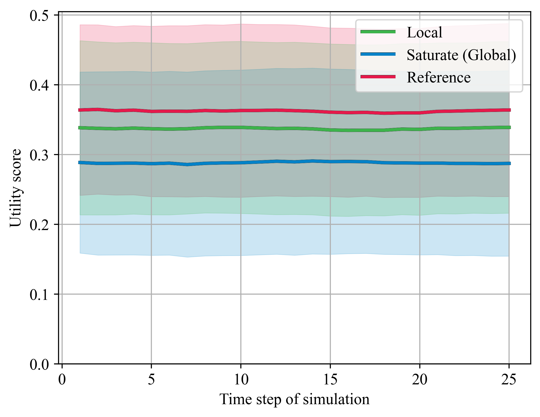
(a)

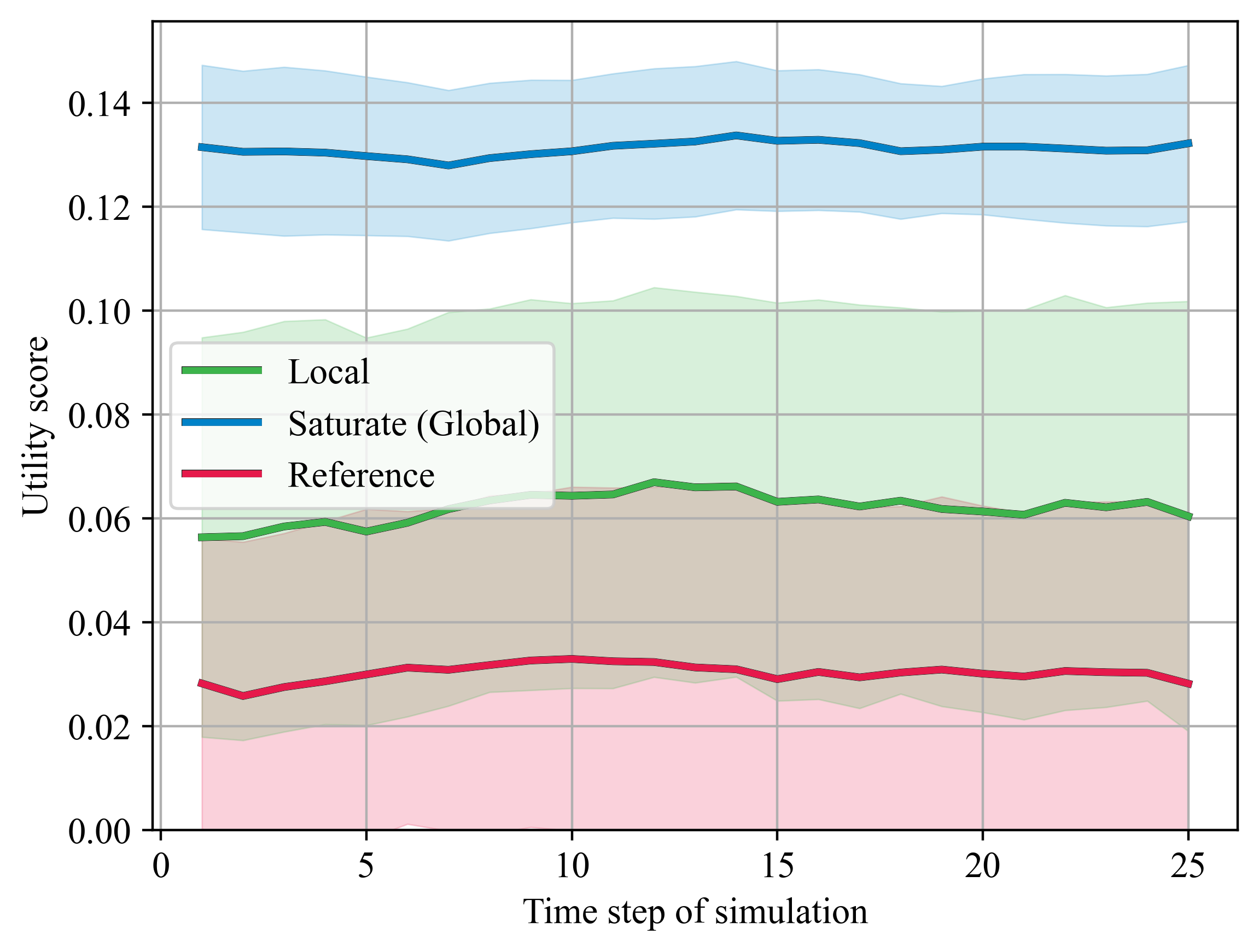
(b)

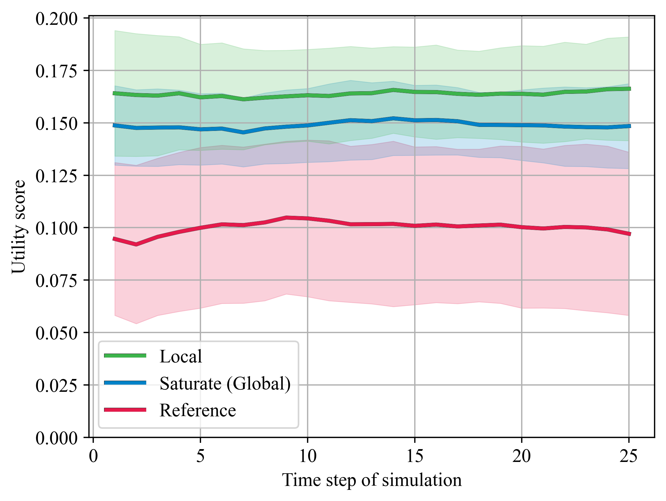
(c)

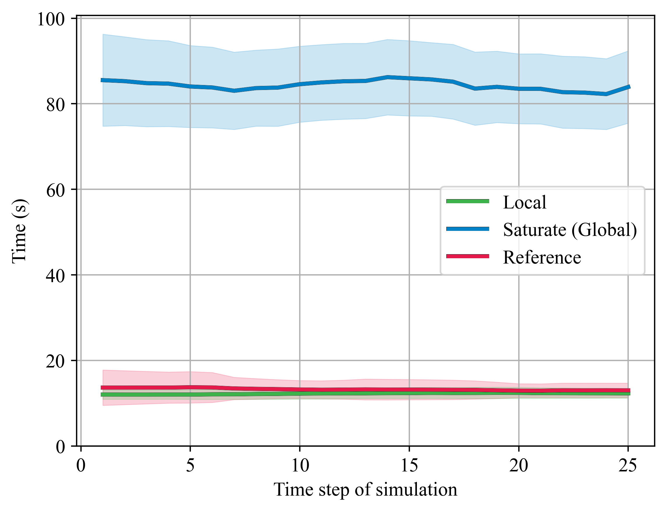
(d)

Fig. 2: The average performances over fifteen runs of the three algorithms focused on optimizing the reference distribution, the global worst-case task, and the local worst-case distribution as guided by the reference distribution, evaluated on the four criteria of reference distribution performance, worst-case task performance, local worst-case distribution performance and the wall-clock time elapsed taken by the algorithm in the construction of the solution in the satellite selection task of Section 6, Subsection 6.1. Local represents the relative entropy-regularized Stochastic Greedy algorithm solving our novel formulation, aiming for local worst-case distributional robustness in the neighborhood of the reference distribution. Saturate (Global) represents the Submodular Saturation Algorithm proposed in [18], aiming for global worst-case task robustness. Reference represents the Stochastic Greedy algorithm being used to directly optimize the utility of the reference distribution. The highlighted areas indicate one standard deviation. The results have been put through a moving average filter with window size 6.

In this section, we will use an application involving a constellation of low Earth orbit (LEO) satellites to test the performance of our three novelly proposed algorithms, namely, the relative entropy-regularized Stochastic Greedy algorithm detailed in Section 4, its application to the online submodular optimization setting detailed in Section 5, and the Saturate with Preference algorithm detailed in Section 3. For the results, we simulate a Walker-Delta constellation parameterized by $i:T/P/f$, where $i$ is the orbit inclination, $T$ is the number of satellites in the constellation, $P$ is the total number of orbital planes of the constellation, and $f$ is the phase difference in between the orbital planes in pattern units[43, 44]. The semi-major axis length of all of the orbits is $8378.1$ kilometers, and the satellites remain Earth-pointing with a field-of-view angle of $\pi/3$ radians. For the testing of all algorithms, we instantiate a constellation with parameters $75^{\circ}:240/12/1$.

In the testing of the relative entropy-regularized Stochastic Greedy and the Saturate with Preference algorithms, we instantiate six distinct tasks that yield six objective functions $f^{1},\ldots,f^{6}$. The objective functions $f^{1},\ldots,f^{5}$ relate to the performance of the algorithms on atmospheric sensing tasks. Each of these tasks involves taking atmospheric readings at a set of five randomly located points on Earth. The atmospheric conditions at these points are described by the Lorenz 63 model[45]. The dynamics at these points are parameterized by values that make the system chaotic. An illustration of one instance of these points is provided in Figure 3, where points labeled $1$ belong to atmospheric reading task $1$ whose performance is indicated by the value of $f^{1}$, and so on. In particular, the utility values $f^{1}(S),\ldots,f^{5}(S)$ of these tasks for a given subset of selected satellites $S$ are proportional to the additive inverse of the mean-squared error (MSE) achieved by the selection $S$ of satellites. The MSE is calculated by estimating the state of each atmospheric sensing point using an unscented Kalman filter [46], and comparing it with the actual values of the atmospheric state at the points of interest. This estimation is highly dependent on whether an atmospheric point is within the field of view of a satellite. Note also that the additive inverse of the MSE is known to be a weak-submodular function.[47, 48]

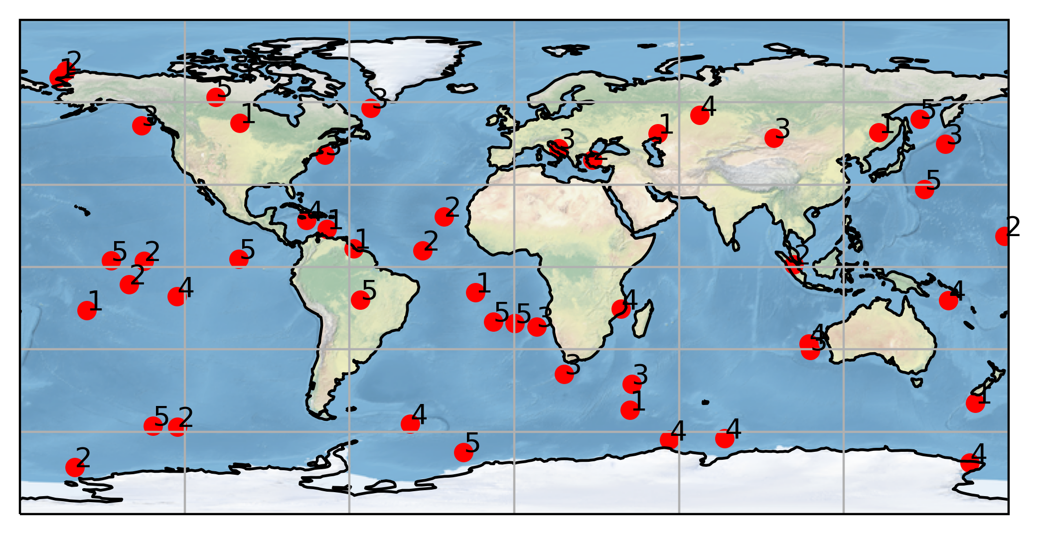
Fig. 3: A selection of atmospheric points of interest for the five atmospheric reading tasks, $f^{1},\ldots,f^{5}$ in one run of the simulation. Each task instantiates five points of interest, for a total of twenty-five points. The labels near the points indicate which atmospheric task a point belongs to.

The sixth and final task, whose performance is related by the objective function $f^{6}$, involves ground coverage of the Earth. The utility value $f^{6}(S)$ of this task is proportional to the Earth coverage achieved by the selected subset $S$ of the satellites in the constellation. The area of coverage is determined based on a grid of the Earth’s surface consisting of cells of width and height $2^{\circ}$. The area of each cell is calculated assuming a spherical Earth. If the center point of a cell on the grid is within the field-of-view of any satellite in the selection, that grid is taken to be covered by the selection.

The utility values of all six tasks $f^{1},\ldots,f^{6}$ are normalized to the range of $[0,1]$, by dividing the utility $f^{i}(S)$ of a selection $S$ on task $f^{i}$ at any time step by $f^{i}(N)$, the maximum utility achievable by selecting the entire ground set at that time step. This ensures that the importance score of an individual task $f^{i}$ is not influenced by the potentially arbitrary value of its utility, and is solely dictated by the weight $Q_{i}$ assigned to it.

We randomly sample a reference distribution $Q$ uniformly from $\Delta_{n}$ to assign an importance score $Q_{i}$ to each task $f^{i}$. Following, we simulate the atmospheric states of the points of interest and the trajectory of the Walker-Delta constellation, for 25 time steps, each corresponding to a time interval of 60 seconds, for 15 runs.

6.1 Relative Entropy-Regularized Stochastic Greedy for Satellite Selection

For the assessment of the relative entropy-regularized Stochastic Greedy algorithm, we compare the performance of the solutions produced by three algorithms, in terms of four distinct performance criteria. For each of the algorithms, we use a cardinality constraint of $K=10$, a sampling set size of $|R|=24$, and a regularization parameter of $\lambda=0.1$, where applicable. The three algorithms compared are as follows:

• Algorithm 1 - Local: The relative-entropy regularized Stochastic Greedy algorithm, that is, the Stochastic Greedy algorithm applied to the maximization of our novel objective function $g(S)=-\lambda\log(\sum_{i=1}^{n}Q_{i}\exp{(-f^{i}(S)/\lambda)}),$ of Problem (25).

• Algorithm 2 - Saturate (Global): The Submodular Saturation Algorithm, which aims to optimize the worst-case scenario in Problem (2).

• Algorithm 3 - Reference: The Stochastic Greedy algorithm, applied to the maximization of the objective function $f(S)=\sum_{i=1}^{n}Q_{i}f^{i}(S)$ of Problem (4), focused on directly optimizing with respect to the reference distribution with no consideration of robustness.

The four performance criteria are as follows:

• Criterion 1: The utility scores with respect to the objective $F_{1}(S)=\sum_{i=1}^{n}Q_{i}f_{i}(S)$, which represents the performance of the algorithms when weighed directly by the reference distribution itself.

• Criterion 2: The utility scores with respect to the objective $F_{2}(S)=\min_{i}f_{i}(S)$, which represents the global worst-case single task performance.

• Criterion 3: The utility scores with respect to the objective $F_{3}(S)=\sum_{i=1}^{n}P^{*}_{i}f_{i}(S)$, where $P^{*}=\arg\!\min_{P}\sum^{n}_{i=1}P_{i}f^{i}(S)+\lambda D_{\text{KL}}(P\;\|\;Q)$, hence representing the local worst-case scenario performance localized to a relative entropy neighborhood of the reference distribution. This criterion may be considered as the benchmark of our novel formulation.

• Criterion 4: The runtime of the algorithm.

The average performances of the three algorithms over 15 runs of the simulation as evaluated by these four criteria are presented in Figure 2.

Several observations may be made looking at these results. Firstly, the designation of Saturate as “too pessimistic” is indeed justified by the results, as seen from Figure 2 (a), where it fails to perform on the reference distribution as it is too focused on worst-case performance. However, it does indeed dominate in worst-case single-task performance over the other two algorithms, as evidenced by Figure 2 (b).

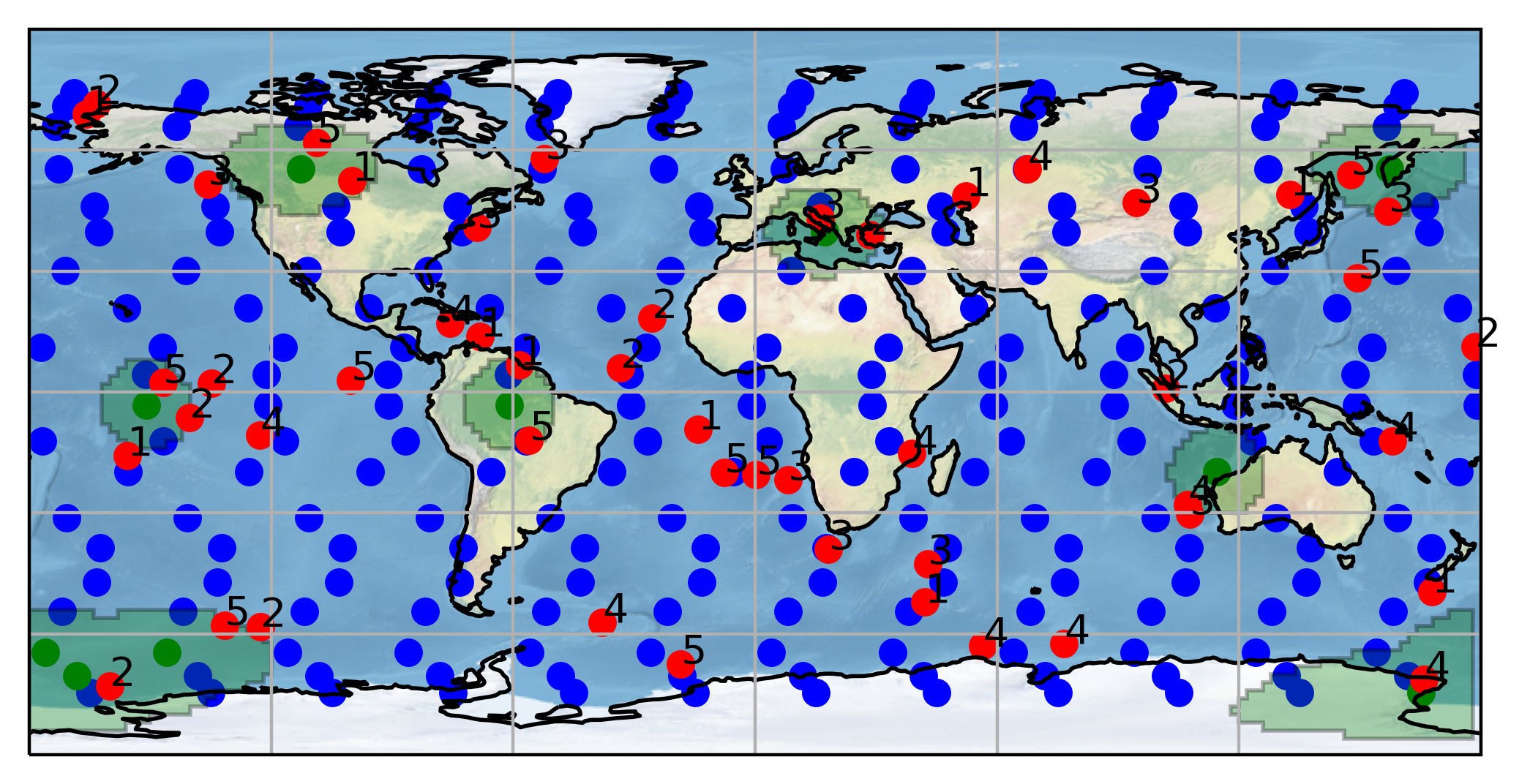
(a)

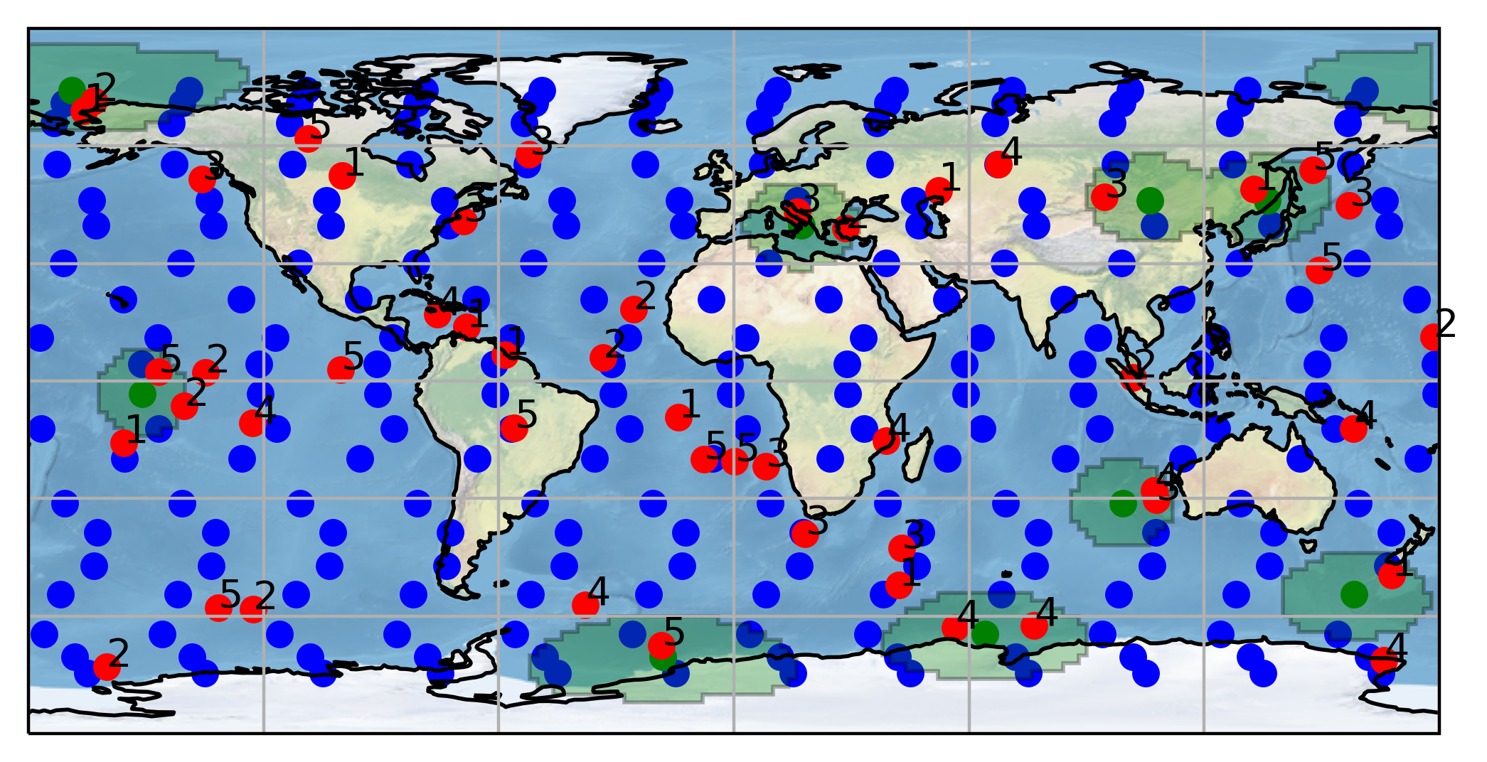
(b)

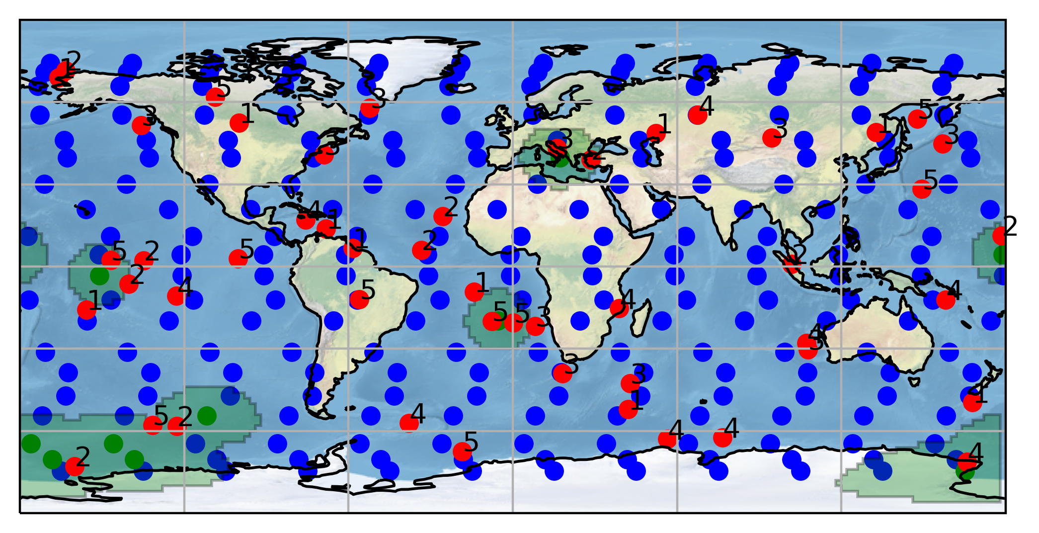
(c)

Fig. 4: The satellites selected by Algorithms 1, 2, and 3 on the 25^th time iteration of one run of the simulation. The red points with their corresponding numbers indicate the atmospheric points of interest and the tasks they belong to. The blue points indicate the satellites in the constellation. The green points indicate the selected satellites at the current time iteration. The highlighted green areas indicate the ground coverage provided by the selected satellites. The reference distribution for this run of the simulation is $Q=[0.022,0.267,0.088,0.087,0.183,0.353].$

Concerning the performance of Algorithm 1 - Local solving our novel formulation, we see from Figure 2 (a) that it has comparable performance on the reference distribution with Algorithm 3 - Reference, which directly optimizes the reference distribution. The usefulness of the Local approach is reflected clearly in Figure 2 (c), where we observe it fulfilling the local distributional robustness that our novel formulation aimed at achieving. Algorithm 1 - Local greatly outperforms Algorithm 3 - Reference and marginally outperforms Saturate on the worst-case scenario within a neighborhood around the reference distribution. However, this marginal surpassing is complemented by the much smaller runtime and computational complexity of the Local approach.

With regard to the wall-clock time taken by the algorithms, as expected, Algorithms 1 and 3 perform identically, as they are essentially the same Stochastic Greedy algorithm. Saturate performs much more poorly, consistently taking many times as much time at each time step. This is explained by the fact that due to its line search-based approach, Saturate uses several runs of the Stochastic Greedy procedure in each of its iterations.

We may conclude from these results that Algorithm 1 - Local, solving our proposed novel formulation, succeeds in constructing a solution that is comparable to Algorithm 3 - Reference in optimizing the performance of the reference distribution, while also achieving local distributional robustness within the neighborhood of the reference distribution. Although Saturate also manages to produce a solution that is more robust against worst-case tasks and achieves decent local distributional robustness, it is much more computationally expensive and has a much longer runtime.

6.2 Saturate with Preference for Satellite Selection

We now turn our attention to the assessment of Algorithm 1, Saturate with Preference. The general setting of the experiments remains similar to the previous subsection, with the same constellation parameters of $75^{\circ}:240/12/1$, and the same objective functions $f^{1},\ldots,f^{6}$. We compare the performance of the selection made by Saturate with Preference, with that of the unmodified Submodular Saturation Algorithm, by looking at the values achieved by the two objective functions that are assigned the highest weight by the random sampling of $Q$. In essence, this allows us to evaluate whether adding the element of preference to SSA works as intended. Indeed, Figure 5 demonstrates that for the two objective functions with the highest priority, Saturate with Preference leads to the selection of a subset that consistently achieves a higher utility score in comparison to SSA. Indeed, Figure 5 demonstrates that Saturate with Preference consistently outperforms SSA in terms of the performance on the objective functions with the highest assigned priority.

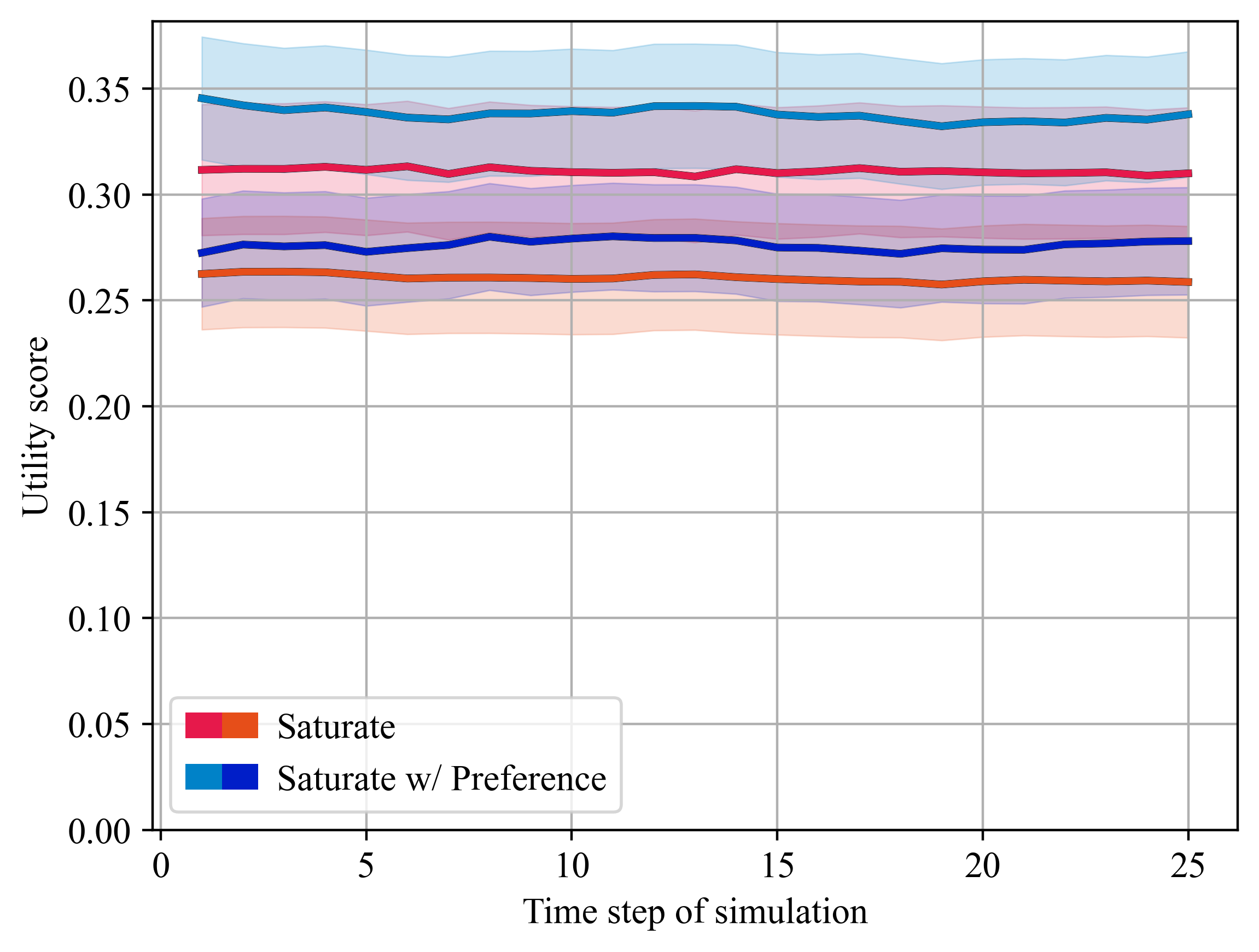
Fig. 5: The average performances over fifteen runs of Saturate with Preference in comparison to the Submodular Saturation Algorithm on the two objective functions with the highest assigned weight. The highlighted areas indicate one tenth standard deviation. The results have been put through a moving average filter with window size 6.

6.3 Application to Online Submodular Optimization

In this subsection, we will assess the performance of the novel formulation (42), which we will call the time-robust (TR) formulation for the sake of brevity, as detailed in Section 5. In summary, the TR formulation aims, using a combination of a momentum-like weighing scheme of the time-varying objective functions in an online setting, along with the idea of relative entropy regularization, to reuse the same selections made in one step over multiple time steps. In this way, it aims to be more cost-efficient in settings where the selection of more diverse elements incurs additional costs.

As a baseline, we choose the standard approach of treating each individual objective function $f_{t}$ observed at time step $t$ as a separate problem and solve it using the Stochastic Greedy algorithm, without any consideration for the conservation of solutions over time steps. Figure 6 demonstrates the comparison of our proposed approach with the time-window size $t_{w}=5$ against the standard approach, in terms of the utility achieved, the wall-clock time taken, and the total number of distinct elements used, i.e., $\lvert\bigcup_{t=0}^{T}S_{t}\rvert$, where $S_{t}$ represents the solution constructed at time step $t$ of the simulation. The results indicate that TR achieves a comparable yet slightly lower utility in comparison to the standard approach. The wall-clock time taken fluctuates in the TR formulation, since with a time-window size of $5$, the algorithm only observes during four of every five time steps and plays its solution, performing all function evaluations on every five time steps, although the total wall-clock time taken is in the same range as the standard approach. However, the total number of distinct elements chosen by the TR formulation is much lower, using less than half the number of distinct elements in comparison to the standard approach.

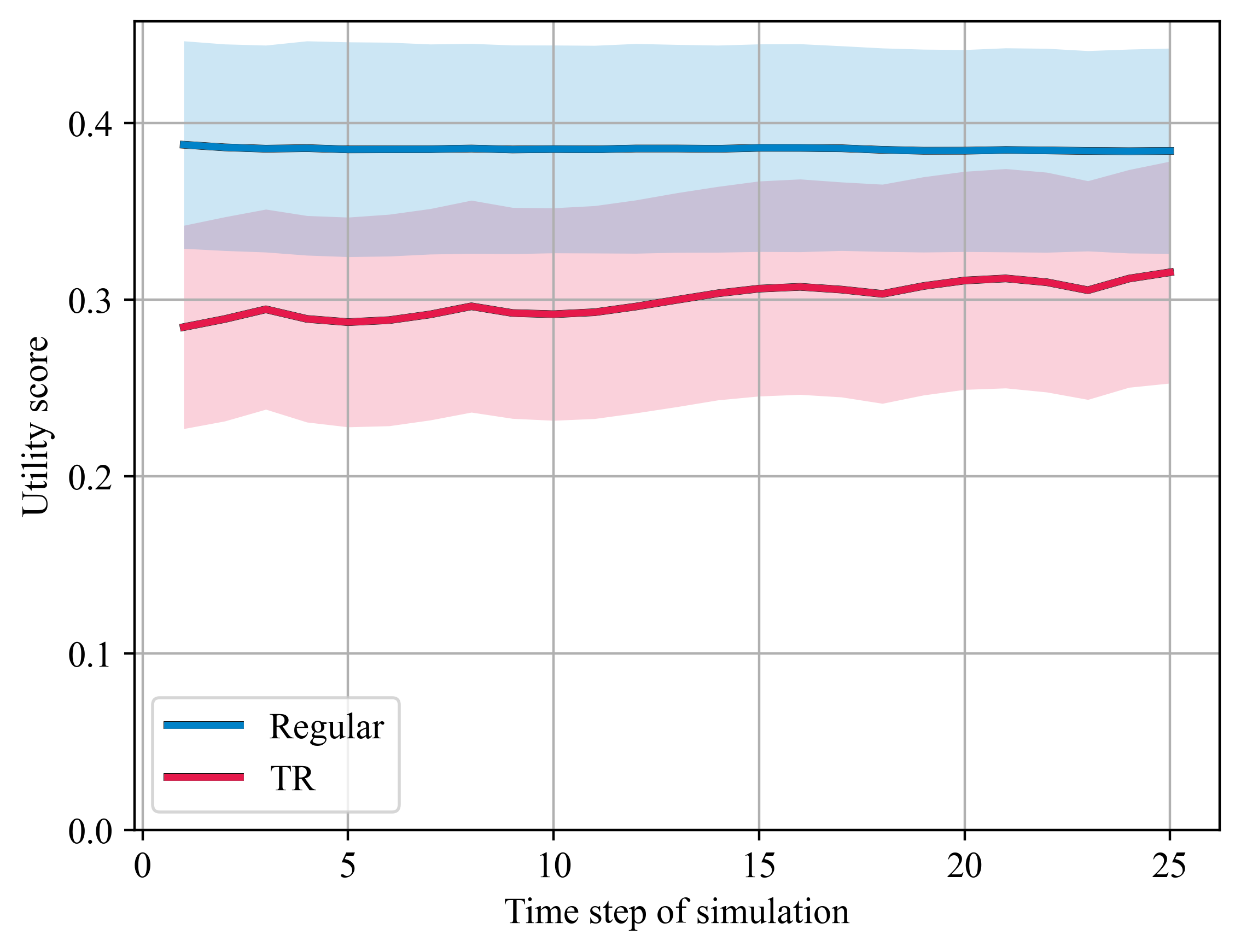
(a)

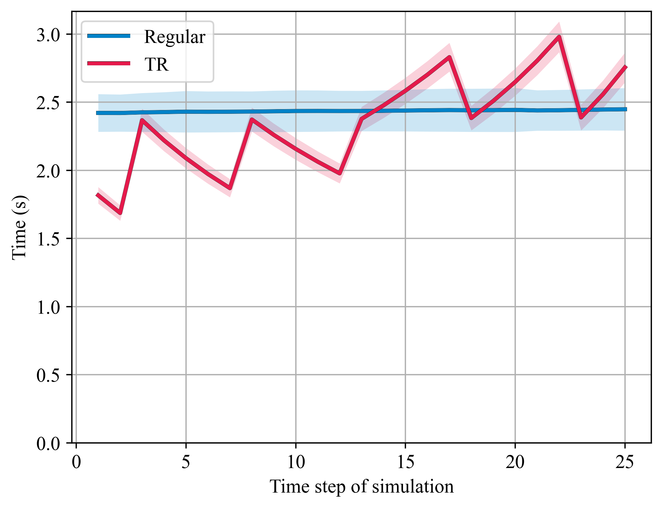
(b)

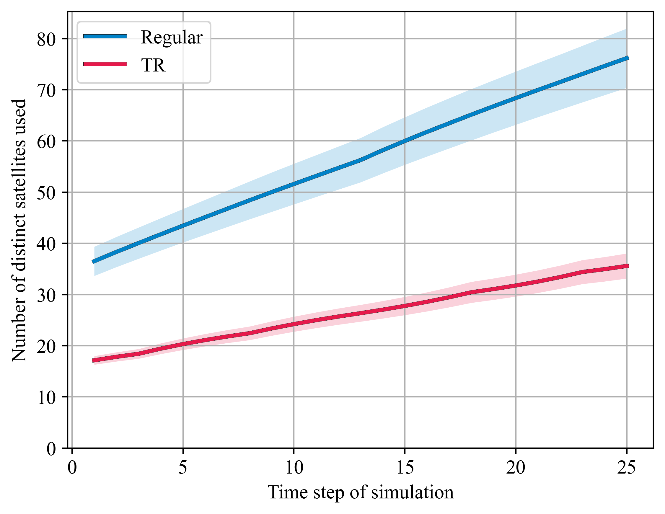
(c)

Fig. 6: The average performances over fifteen runs of the two algorithms in the online task detailed in Section 6, 6.3. The comparison criteria are the utility achieved, the wall-clock time taken, and the total number of distinct elements used. Regular represents the standard approach of solving each objective function $f_{t}$ observed at time step $t$ independently of the previous objective functions observed, using the Stochastic Greedy algorithm. TR represents the time-robust formulation detailed in Section 5, with a time-window size $t_{w}=5$. The highlighted areas indicate one standard deviation. The results have been put through a moving average filter with size 6.

6.4 Practical Application: Image Summarization

As a final demonstration using a more day-to-day application involving machine learning and signal processing, we apply the proposed method to image summarization. We tackle the case detailed in [30], which, in short, involves selecting the most representative $K\leq\lvert N\rvert$ images out of a dataset $N=\{1,2,\ldots,\lvert N\rvert\}$ of indexed images. More formally, for a selection $S\subseteq N$ of images, one can evaluate the utility $f^{i}(S)$ of each image $i\in N$ through its similarity to the closest image in the selection by:

$$f^{i}(S)=1-\min_{e\in S}d(i,e),$$ (43)

where $d(i,e)$ designates some measure of distance between images $i$ and $e$. Replicating the setting in the aforementioned work [30], we use the $\lvert N\rvert=819$-image Pokemon dataset[49], using image embeddings calculated with an AlexNet[29] trained on the ImageNet dataset[50]. We use the normalized cosine distance

$$d(i,e)=\frac{v_{i}\cdot v_{e}}{\lVert v_{i}\rVert\lVert v_{e}\rVert}+\min_{(e,e^{{}^{\prime}})\in N^{2}}\frac{v_{e}\cdot v_{e^{{}^{\prime}}}}{\lVert v_{e}\rVert\lVert v_{e^{{}^{\prime}}}\rVert}.$$ (44)

The average results obtained from fifteen runs of the algorithms, where in each the reference distribution $Q$ is the uniform distribution, are demonstrated in Figure 7. We observe that our proposed Local algorithm outperforms Saturate for nearly all values of the cardinality constraint $K$ on the reference distribution and on the local worst-case distribution, while also taking significantly less computation time, as evidenced by the results of the previous experiments. Regarding the performance on the worst-case task, Saturate only outperforms our algorithm within the cardinality constraint range of $K=1$ to $K=5$, but then both algorithms show virtually the same performance, again, with the Local algorithm being much less computationally expensive.

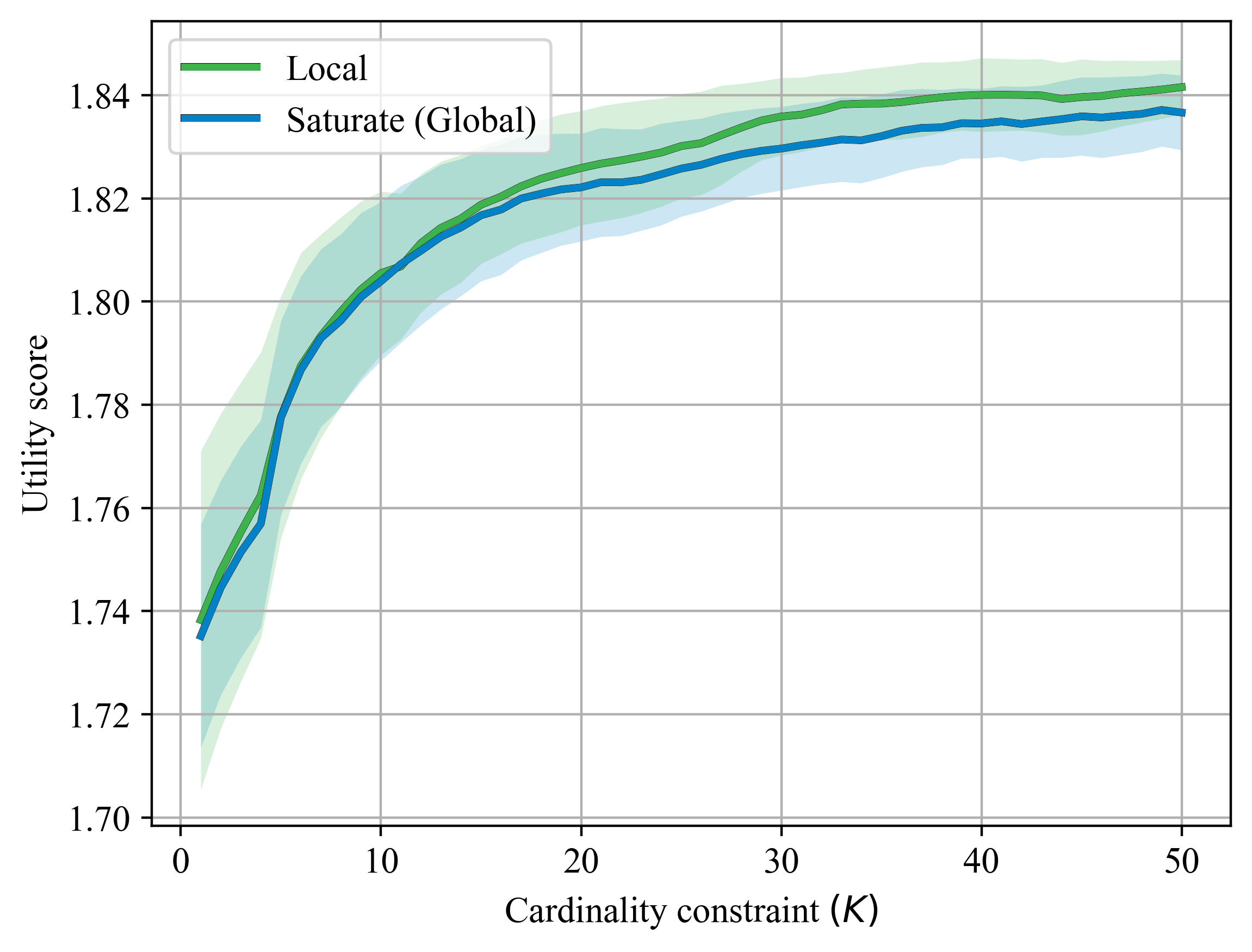
(a)

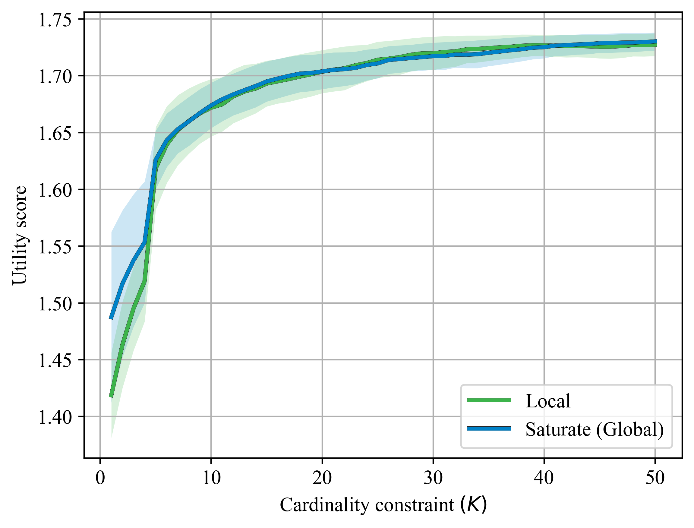
(b)

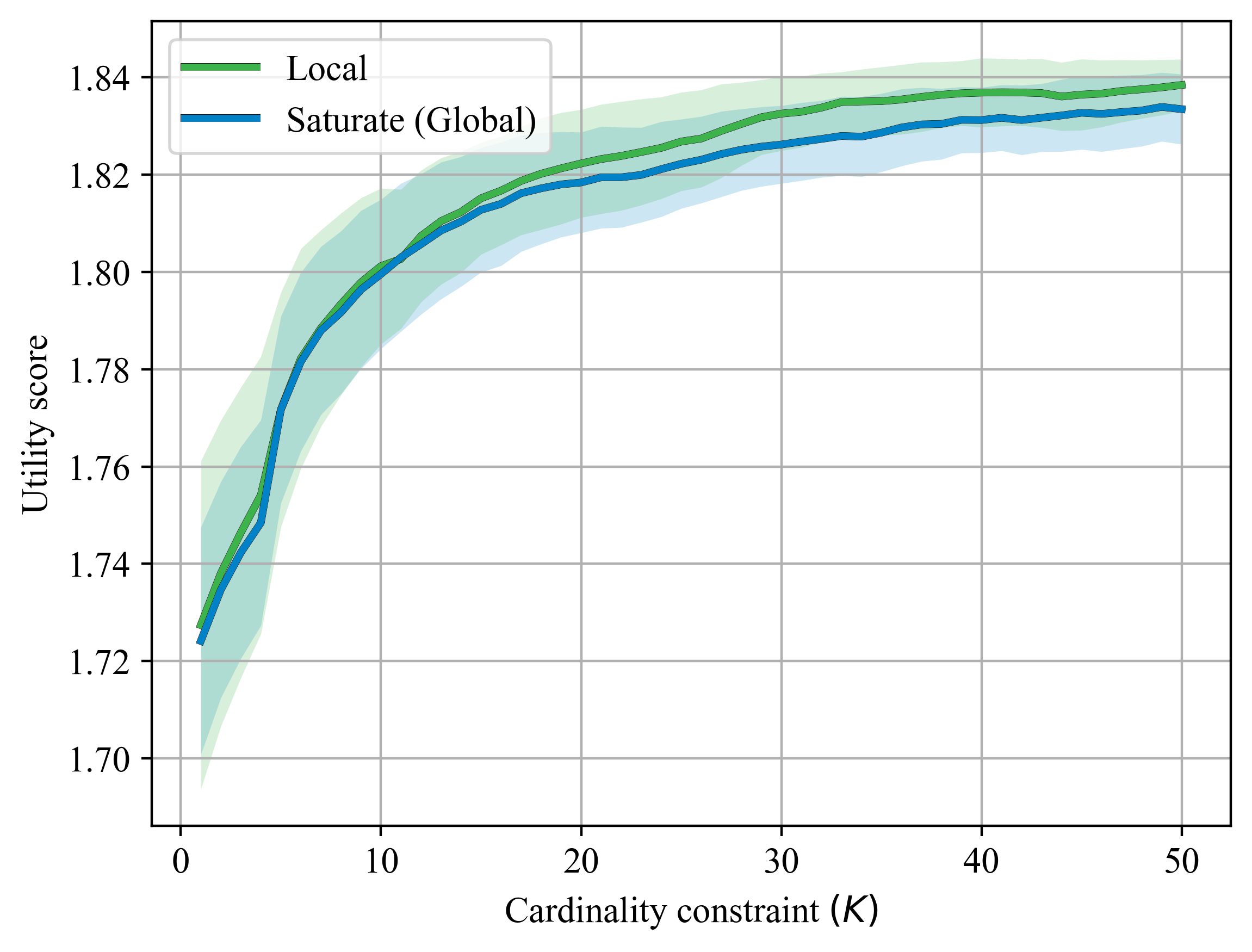
(c)

Fig. 7: The average performances over fifteen runs of the two algorithms focused on optimizing the global worst-case task, and the local worst-case distribution as guided by the reference distribution, evaluated on the three criteria of reference distribution performance, worst-case task performance, and local worst-case distribution performance in the image summarization task of Section 6, Subsection 6.4. Local represents the relative entropy-regularized Stochastic Greedy algorithm solving our novel formulation, aiming for local worst-case distributional robustness in the neighborhood of the reference distribution. Saturate (Global) represents the Submodular Saturation Algorithm proposed in [18], aiming for global worst-case task robustness. The highlighted areas indicate one standard deviation. The results have been put through a moving average filter with window size 6.

7 Conclusion

We proposed the novel formulation of Problem (14) to find a solution that is locally distributionally robust in the neighborhood of a reference distribution, assign an importance score to each task in a multi-task objective, using various statistical distances as a regularizer. The $\ell^{1}$ and $\ell^{\infty}$ distances led to the proposal of the Saturate with Preference algorithm, which incorporates an element of preference into the standard Submodular Saturation Algorithm. Afterward, we demonstrated that using relative entropy as a regularizer, through duality, one can show that this novel formulation is equivalent to Problem (25). Then, we proved that this dual formulation gives rise to another normalized, monotone nondecreasing submodular function, which can be optimized with standard methods such as the Stochastic Greedy algorithm, enjoying theoretical guarantees such as Theorem (1). We proposed an application of the relative entropy regularized to online submodular optimization, through the use of a momentum-like weighing of the objective functions observed at each time step. We then experimentally corroborated our results for all three of the proposed settings, motivated by a practical scenario involving a sensor selection problem within a simulation of LEO satellites. For the relative entropy regularization setting, we compared our algorithm with two other algorithms focused on optimizing the performance of the worst-case task, and on directly optimizing the performance reference distribution itself. We concluded that solving our novel formulation produces a solution that performs well on the reference distribution, is locally distributionally robust, and is quick in terms of computation time. For the Saturate with Preference setting, we showed that our algorithm consistently outperforms the standard Submodular Saturation Algorithm in terms of the performance on the objective functions with the highest assigned preference. For the application to the online submodular optimization setting, we demonstrated that our algorithm achieves a comparable utility to the regular method of solving each observed objective function at the moment of its observation, with a comparable wall-clock time taken. However, it does so by using a much smaller total number of distinct satellites. Finally, for a more general, real-life application of the proposed relative entropy-regularized algorithm, we tackled an image summarization task based on contemporary neural network usage.

References

- [1] J. Edmonds, “Submodular functions, matroids, and certain polyhedra,” in Combinatorial Optimization—Eureka, You Shrink! Papers Dedicated to Jack Edmonds 5th International Workshop Aussois, France, March 5–9, 2001 Revised Papers, pp. 11–26, Springer, 2003.
- [2] S. Fujishige, Submodular functions and optimization. Elsevier, 2005.
- [3] R. K. Iyer and J. A. Bilmes, “Submodular optimization with submodular cover and submodular knapsack constraints,” Advances in neural information processing systems, vol. 26, 2013.
- [4] A. Krause and D. Golovin, “Submodular function maximization.,” Tractability, vol. 3, pp. 71–104, 2014.
- [5] N. Buchbinder, M. Feldman, J. S. Naor, and R. Schwartz, “Submodular maximization with cardinality constraints,” in Proceedings of the Twenty-Fifth Annual ACM-SIAM Symposium on Discrete Algorithms, SODA ’14, (USA), p. 1433–1452, Society for Industrial and Applied Mathematics, 2014.
- [6] S. Dughmi, T. Roughgarden, and M. Sundararajan, “Revenue submodularity,” in Auctions, Market Mechanisms and Their Applications (S. Das, M. Ostrovsky, D. Pennock, and B. Szymanksi, eds.), (Berlin, Heidelberg), pp. 89–91, Springer Berlin Heidelberg, 2009.
- [7] A. S. Schulz and N. A. Uhan, “Approximating the least core value and least core of cooperative games with supermodular costs,” Discrete Optimization, vol. 10, no. 2, pp. 163–180, 2013.
- [8] H. Lin and J. Bilmes, “A class of submodular functions for document summarization.,” vol. 1, pp. 510–520, 01 2011.
- [9] F. Bach, “Structured sparsity-inducing norms through submodular functions,” vol. 23, 08 2010.
- [10] J. Gillenwater, A. Kulesza, and B. Taskar, “Near-optimal map inference for determinantal point processes,” Advances in Neural Information Processing Systems, vol. 4, pp. 2735–2743, 01 2012.
- [11] R. Kumar, B. Moseley, S. Vassilvitskii, and A. Vattani, “Fast greedy algorithms in mapreduce and streaming,” vol. 2, pp. 1–10, 07 2013.
- [12] R. Iyer and J. Bilmes, “Submodular Point Processes with Applications to Machine learning,” in Proceedings of the Eighteenth International Conference on Artificial Intelligence and Statistics (G. Lebanon and S. V. N. Vishwanathan, eds.), vol. 38 of Proceedings of Machine Learning Research, (San Diego, California, USA), pp. 388–397, PMLR, 09–12 May 2015.
- [13] A. Gotovos, H. Hassani, and A. Krause, “Sampling from probabilistic submodular models,” in Advances in Neural Information Processing Systems (C. Cortes, N. Lawrence, D. Lee, M. Sugiyama, and R. Garnett, eds.), vol. 28, Curran Associates, Inc., 2015.
- [14] V. Kolmogorov and R. Zabin, “What energy functions can be minimized via graph cuts?,” IEEE Transactions on Pattern Analysis and Machine Intelligence, vol. 26, no. 2, pp. 147–159, 2004.
- [15] Y. Liu, K. Wei, K. Kirchhoff, Y. Song, and J. Bilmes, “Submodular feature selection for high-dimensional acoustic score spaces,” in 2013 IEEE International Conference on Acoustics, Speech and Signal Processing, pp. 7184–7188, 2013.
- [16] A. Das and D. Kempe, “Submodular meets spectral: Greedy algorithms for subset selection, sparse approximation and dictionary selection,” in Proceedings of the 28th International Conference on International Conference on Machine Learning, ICML’11, (Madison, WI, USA), p. 1057–1064, Omnipress, 2011.
- [17] B. W. Dolhansky and J. A. Bilmes, “Deep submodular functions: Definitions and learning,” in Advances in Neural Information Processing Systems (D. Lee, M. Sugiyama, U. Luxburg, I. Guyon, and R. Garnett, eds.), vol. 29, Curran Associates, Inc., 2016.
- [18] A. Krause, H. B. McMahan, C. Guestrin, and A. Gupta, “Robust submodular observation selection,” Journal of Machine Learning Research, vol. 9, no. 93, pp. 2761–2801, 2008.
- [19] M. Shamaiah, S. Banerjee, and H. Vikalo, “Greedy sensor selection: Leveraging submodularity,” in 49th IEEE Conference on Decision and Control (CDC), pp. 2572–2577, 2010.
- [20] A. Krause and C. Guestrin, “Near-optimal observation selection using submodular functions,” in Proceedings of the 22nd National Conference on Artificial Intelligence - Volume 2, AAAI’07, p. 1650–1654, AAAI Press, 2007.
- [21] E. Mossel and S. Roch, “On the submodularity of influence in social networks,” pp. 128–134, ACM, 6 2007.
- [22] G. L. Nemhauser, L. A. Wolsey, and M. L. Fisher, “An analysis of approximations for maximizing submodular set functions—i,” Mathematical programming, vol. 14, pp. 265–294, 1978.
- [23] L. Lovász, Submodular functions and convexity, pp. 235–257. Berlin, Heidelberg: Springer Berlin Heidelberg, 1983.
- [24] I. Bogunovic, S. Mitrović, J. Scarlett, and V. Cevher, “Robust submodular maximization: A non-uniform partitioning approach,” in Proceedings of the 34th International Conference on Machine Learning (D. Precup and Y. W. Teh, eds.), vol. 70 of Proceedings of Machine Learning Research, pp. 508–516, PMLR, 06–11 Aug 2017.
- [25] G. Lan, Stochastic Convex Optimization, pp. 113–220. Cham: Springer International Publishing, 2020.
- [26] H.-G. Beyer and B. Sendhoff, “Robust optimization – a comprehensive survey,” Computer Methods in Applied Mechanics and Engineering, vol. 196, no. 33, pp. 3190–3218, 2007.
- [27] A. Ben-Tal, L. El Ghaoui, and A. Nemirovski, Robust optimization, vol. 28. Princeton university press, 2009.
- [28] A. Ben-Tal and A. Nemirovski, “Robust optimization–methodology and applications,” Mathematical programming, vol. 92, pp. 453–480, 2002.
- [29] R. Udwani, “Multi-objective maximization of monotone submodular functions with cardinality constraint,” in Advances in Neural Information Processing Systems (S. Bengio, H. Wallach, H. Larochelle, K. Grauman, N. Cesa-Bianchi, and R. Garnett, eds.), vol. 31, Curran Associates, Inc., 2018.
- [30] C. Malherbe and K. Scaman, “Robustness in multi-objective submodular optimization: a quantile approach,” in International Conference on Machine Learning, pp. 14871–14886, PMLR, 2022.
- [31] M. Staib, B. Wilder, and S. Jegelka, “Distributionally robust submodular maximization,” in Proceedings of the Twenty-Second International Conference on Artificial Intelligence and Statistics (K. Chaudhuri and M. Sugiyama, eds.), vol. 89 of Proceedings of Machine Learning Research, pp. 506–516, PMLR, 16–18 Apr 2019.
- [32] S. P. Boyd and L. Vandenberghe, Convex Optimization. Cambridge University Press, 2014.
- [33] T. Powers, J. A. Bilmes, S. Wisdom, D. W. Krout, and L. E. Atlas, “Constrained robust submodular optimization,” 2016.
- [34] V. Tzoumas, A. Jadbabaie, and G. J. Pappas, “Robust and adaptive sequential submodular optimization,” IEEE Transactions on Automatic Control, vol. 67, no. 1, pp. 89–104, 2022.
- [35] W. Wiesemann, D. Kuhn, and M. Sim, “Distributionally robust convex optimization,” Operations Research, vol. 62, no. 6, pp. 1358–1376, 2014.
- [36] Q. Qi, Z. Guo, Y. Xu, R. Jin, and T. Yang, “An online method for a class of distributionally robust optimization with non-convex objectives,” 2021.
- [37] M. Minoux, “Accelerated greedy algorithms for maximizing submodular set functions,” in Optimization Techniques (J. Stoer, ed.), (Berlin, Heidelberg), pp. 234–243, Springer Berlin Heidelberg, 1978.
- [38] B. Mirzasoleiman, A. Badanidiyuru, A. Karbasi, J. Vondrák, and A. Krause, “Lazier than lazy greedy,” in Proceedings of the AAAI Conference on Artificial Intelligence, vol. 29, 2015.
- [39] D. Bertsimas and J. Tsitsiklis, Introduction to linear optimization. Athena Scientific, 1997.
- [40] D. P. Kingma and J. Ba, “Adam: A method for stochastic optimization,” arXiv preprint arXiv:1412.6980, 2014.
- [41] R. Das, A. Acharya, A. Hashemi, S. Sanghavi, I. S. Dhillon, and U. Topcu, “Faster non-convex federated learning via global and local momentum,” in Uncertainty in Artificial Intelligence, pp. 496–506, PMLR, 2022.
- [42] R. S. Sutton and A. G. Barto, Reinforcement learning: An introduction. 2018.
- [43] M. Hibbard, A. Hashemi, T. Tanaka, and U. Topcu, “Randomized greedy algorithms for sensor selection in large-scale satellite constellations,” Proceedings of the American Control Conference, 2023.
- [44] J. G. Walker, “Satellite Constellations,” Journal of the British Interplanetary Society, vol. 37, p. 559, Dec. 1984.
- [45] E. N. Lorenz, “Deterministic nonperiodic flow,” Journal of Atmospheric Sciences, vol. 20, no. 2, pp. 130 – 141, 1963.
- [46] Y. Bar-Shalom, X. Li, and T. Kirubarajan, “Estimation with applications to tracking and navigation: Theory, algorithms and software,” 2001.
- [47] A. Hashemi, M. Ghasemi, H. Vikalo, and U. Topcu, “Randomized greedy sensor selection: Leveraging weak submodularity,” IEEE Transactions on Automatic Control, vol. 66, no. 1, pp. 199–212, 2021.
- [48] A. Hashemi, M. Ghasemi, H. Vikalo, and U. Topcu, “A randomized greedy algorithm for near-optimal sensor scheduling in large-scale sensor networks,” in 2018 Annual American Control Conference (ACC), pp. 1027–1032, 2018.
- [49] S. Churchill, “Pokemon images dataset,” 2017.
- [50] J. Deng, W. Dong, R. Socher, L.-J. Li, K. Li, and L. Fei-Fei, “Imagenet: A large-scale hierarchical image database,” in 2009 IEEE Conference on Computer Vision and Pattern Recognition, pp. 248–255, 2009.