Thermal noise squeezing and amplification in parametrically driven resonators

Abstract

Here we propose several methods with increasing precision for analytically estimating white noise squeezing in the frequency domain of classical parametrically-driven resonators with added noise. The analytical model is based on obtaining the response of the resonator to the added noise using Green’s function. The response consists of three parts: elastic, down, and up parametric conversions. We obtain the Green’s function approximately using the first-order averaging method or exactly, in principle, using Floquet theory. We characterize the noise squeezing by calculating the statistical properties of the real and imaginary parts of the Fourier transform of the resonator response to added noise. Furthermore, we observe that the squeezing effects occur only at half the parametric pump frequency. Due to correlation, the squeezing limit of $-6$ dB can be reached even with detuning around resonance near the instability threshold. Additionally, we validate some of our theoretical predictions of squeezing with the results obtained from the numerical integration of the stochastic differential equations of our model. We also applied our techniques to investigate squeezing in a pair of coupled parametric and harmonic resonators with a single noise input. The results obtained from Floquet theory can be applied generally to coupled resonators in which at least one of the resonators is parametrically modulated.

I Introduction

Parametric resonators and amplifiers have been implemented in many different systems of physics and engineering such as MEMS/NEMS Karabalin et al. (2009); Thomas et al. (2013); Prakash et al. (2012), optomechanics He et al. (2023), Josephson Junctions Castellanos-Beltran et al. (2008); B. H. Eom, P. K. Day, H. G. LeDuc, and Zmuidzinas (2012), atomic force microscopy Moreno-Moreno et al. (2006), ion traps Paul (1990), etc. Driving parametrically a harmonic resonator is a way to tune its quality factor Miller et al. (2018); Lee et al. (2022). A very high effective $Q$ can thus be obtained. Hence, these amplifiers can achieve very high gains and a very narrow gain bandwidth. The narrow band decreases the effect of fluctuations due to added noise. Further decrease of fluctuations can be achieved when noise squeezing techniques are used. These techniques have been used in high-precision position measurements Szorkovszky et al. (2013) and also to measure small forces and helped detect gravitational waves in the LIGO experiment Kimble et al. (2001); Chen (2013); Abbott et al. (2016).

In a seminal paper in 1991, Rugar and Grütter Rugar and Grütter (1991) experimentally observed the effect of thermomechanical noise squeezing of flexural vibrations of a clamped microcantilever that was parametrically excited at twice the fundamental mode frequency. The squeezing effect was observed and measured with the aid of a two-phase lock-in amplifier (LIA), in which the signal of the vibrations was split in two channels in quadrature with one another. In one channel it was multiplied by a cosine and in the other by a sine at half the pump frequency. Subsequently, an integration was performed over a long time compared to the vibration period and the result is divided by the integration time interval. Hence, the two LIA outputs were basically proportional to the real and imaginary parts of the Fourier transform of the signal at half the pump frequency. It was observed by the authors that when the parametric pump was turned on, the fluctuations increased in one quadrature phase, while in the other quadrature they decreased. This squeezing effect was most noticeable in the stable zone near the transition line of the first parametric instability with the parametric pump frequency set at twice the fundamental mode of the resonator. They reached a $-4.9$ dB amplitude deamplification experimentally and commented that a lower bound of $-6$ dB could be reached at the parametric instability threshold. No theoretical model based on stochastic differential equations was proposed by the authors to explain this thermal noise squeezing effect though.

DiFilippo et al. DiFilippo et al. (1992) developed further noise squeezing techniques and applied them to single ion mass spectroscopy based on classical harmonic and anharmonic oscillators parametrically driven at twice the natural frequency only. They proposed theoretical explanations for squeezing based on a Hamiltonian (area preserving) time evolution of a Gaussian distribution of initial values, thus neglecting dissipation and noise. They proposed two models of parametric squeezing which they called amplitude and quadrature squeezing. In amplitude squeezing, the stretching and squeezing of the initial distribution is a consequence of the strengthening nonlinear spring constant of the parametrically driven Duffing oscillator model they used that causes higher energy states to oscillate at higher frequencies than lower energy states. On the other hand, in quadrature squeezing, the squeezing and stretching that occurs in a dissipationless parametric oscillator pumped at twice its natural frequency is due to the inherent instability of the fixed point (a saddle point) of the averaged equations of motion. Thus, their model cannot be used to explain the sub-threshold thermomechanical noise squeezing and $-6$ dB deamplification limit observed experimentally by Rugar and Grütter. Subsequently Natarajan et al. Natarajan et al. (1995) proposed another squeezing technique that was applied to increase precision of amplitude measurement of oscillations of a single ion in a Penning trap, whose fixed point was made stable by parametric pumping. We point out that, unlike Floquet theory, the averaging method cannot be properly applied to explain squeezing in this system since without pumping there are no oscillations. In Ref. Cleland (2005), Cleland investigated thermal noise squeezing in a parametric resonator by analyzing the noise spectral density (NSD) in two channels in quadrature of the slowly-varying variables based on Louisell’s coupled mode method and by making subsequent phase averages over the external ac drive, not via the analysis of stochastic differential equations. Again, the results were limited to resonance when half the pump frequency is equal to the natural frequency of a single-degree-of-freedom parametric resonator.

There have been attempts at increasing thermal noise squeezing beyond the $-6$ dB level using several different systems and methods such as two-mode coupling in nanomechanical resonators Mahboob et al. (2014); Patil et al. (2015); Pontin et al. (2016); Singh et al. (2018), multi-mode coupling Zhao et al. (2021), feedback Vinante and Falferi (2013); Poot et al. (2015); Sonar et al. (2018), and nonlinear squeezing Almog et al. (2007); Huber et al. (2020). All methods used are approximate solutions adapted to each problem, none of them being general. Instead, what we propose here is a theoretical method that could be applied to all linear parametric amplifier systems without feedback. In addition to that, our method can be applied to nonlinear squeezing if the added noise can be considered as a small perturbation. In nonlinear squeezing, the response to noise will be given by a parametrically driven system in which the pump is given by a stable limit cycle solution of the unperturbed dynamical system (i.e. without added noise) Wiesenfeld (1985). The only systems that cannot be covered by our present analysis are those with feedback, since their dynamics is given by stochastic difference-differential equations.

Here, we propose a theoretical model based on stochastic differential equations that accounts for thermal noise squeezing such as first observed by Rugar and Grütter in a classical parametrically driven resonator. Qualitatively, thermal noise squeezing can be linked to a universal behavior of parametrically driven oscillators. Due to the constraint imposed by the Liouville’s formula, the two Floquet multipliers are either a complex conjugate pair whose module is less than or equal to 1 or are two different real numbers whose product is less than or equal to 1. The equality occurs when there is no dissipation. After the complex conjugate pair becomes real, with increasing pump amplitude, one Floquet multiplier increases in magnitude, while the other decreases, until the instability threshold is achieved when one of the multipliers becomes of magnitude 1. This is a general feature of any parametrically-driven damped harmonic oscillator whatever the periodic parametric drive. When the Floquet exponents are real, the thermal noise squeezing is enhanced due to the existence of two different effective dissipation rates: one larger and the other smaller than the equilibrium dissipation rate.

We begin our theoretical modeling for noise squeezing by writing down the frequency-domain response to added white noise of the parametrically modulated resonator. This response is split in three parts: one is an elastic scattering, and the other two are parametric up and down conversions. The elastic response can be obtained from the time translation invariant part of the Green’s function. The other responses are due to the Green’s function part that is not symmetric under time translation. Subsequently, we split the resonator response into real and imaginary parts. Afterwards, we obtain the average fluctuations of the real and imaginary parts and the correlation between them. For a generic pump phase, we obtain these statistical measures from a bivariate Gaussian distribution with correlation. By an appropriate change of coordinates, one can transform from this distribution to an uncorrelated product of two univariate Gaussian distributions. From the latter distributions, we obtain the length and width of the distribution of data points equivalent to the cloud obtained from the LIA measurements by Rugar and Grütter. Alternatively, one can choose one pump phase in which there is no correlation. We develop the approximate theory of noise squeezing in which the Green’s function of the parametrically-modulated resonator is obtained in the first-order averaging method. Finally, we also develop an exact theory of noise squeezing based on Floquet theory. We point out that with this general approach, in principle, one can extend the noise squeezing theory to any number of coupled parametrically modulated resonators with added noise.

The remainder of this paper is organized as follows: in Sec. II we state our problem and develop the analytical model of noise squeezing based on the first-order averaging approximation (in Subsec. II.1), and on Floquet theory (in Subsec. II.2). In Sec. III we present and discuss our results. In Sec. IV we draw our conclusions.

II Model and Analysis

We investigate here the effect of added white noise on the parametrically-driven resonator Batista (2011). Its stochastic differential equation can be written as

$$\ddot{x}=-x-\gamma\dot{x}+F_{p}\cos(2\omega t+\varphi_{p})\;x+r(t),$$ (1)

where $\gamma$ is the dissipation rate, $F_{p}$ is the pump amplitude, $\omega$ is half the pump frequency, $\varphi_{p}$ is the pump phase, and $r(t)$ is a Gaussian white noise that satisfies the statistical averages $\langle r(t)\rangle=0$ and $\langle r(t)r(t^{\prime})\rangle=2D\delta(t-t^{\prime})$, where $D$ is the noise level. Below, we tackle the problem of understanding thermal noise squeezing with two approaches: one using the first-order averaging approximation and the other using Floquet theory.

II.1 Noise squeezing in the 1st-order averaging approximation

The response in frequency space of the parametrically driven resonator to added white noise Batista et al. (2022) is given by

$$\tilde{x}(\nu) =\tilde{G}_{0}(\nu)\tilde{r}(\nu)-\frac{\beta}{2\omega}\left[\frac{e^{-i\varphi_{p}}\tilde{r}(\nu-2\omega)}{[\rho_{-}+i(\nu-\omega)][\rho_{+}+i(\nu-\omega)]}+\frac{e^{i\varphi_{p}}\tilde{r}(\nu+2\omega)}{[\rho_{-}+i(\nu+\omega)][\rho_{+}+i(\nu+\omega)]}\right]$$ (2)

$$=\tilde{G}_{0}(\nu)\tilde{r}(\nu)+\Gamma(\nu)\tilde{r}(\nu-2\omega)+\Gamma^{*}(-\nu)\tilde{r}(\nu+2\omega),$$

where we used the shorthand notations

$$\Gamma(\nu) =-\frac{\beta}{2\omega}\frac{e^{-i\varphi_{p}}}{[\rho_{-}+i(\nu-\omega)][\rho_{+}+i(\nu-\omega)]},$$ (3)

$$\tilde{G}_{0}(\nu) \approx\frac{1}{2\omega}\left[\frac{\delta+\nu-\omega+i\gamma/2}{[\rho_{-}+i(\nu-\omega)][\rho_{+}+i(\nu-\omega)]}+\frac{\delta-\nu-\omega-i\gamma/2}{[\rho_{-}+i(\nu+\omega)][\rho_{+}+i(\nu+\omega)]}\right],$$ (4)

in which $\rho_{\pm}=-\gamma/2\pm\kappa$ are the Floquet exponents in the first-order averaging approximation, where $\kappa=\sqrt{\beta^{2}-\delta^{2}}$, $\beta=-F_{p}/4\omega$, $\delta=\Omega/2\omega$, and $\Omega=1-\omega^{2}$ Batista (2012). Near the onset of instability, at $\nu=\omega$, we have

$$\tilde{G}_{0}(\omega)\approx\frac{1}{2\omega}\left[\frac{\delta+i\gamma/2}{\rho_{-}\rho_{+}}+\frac{\delta-2\omega-i\gamma/2}{(\rho_{-}+2i\omega)(\rho_{+}+2i\omega)}\right]\approx\frac{\delta+i\gamma/2}{2\omega\rho_{-}\rho_{+}}.$$ (5)

Here, we use the following notation for Fourier transforms

$$\tilde{f}(\nu)=\int_{-\infty}^{\infty}e^{i\nu t}f(t)\,dt.$$

We are now going to investigate the thermal noise squeezing phenomenon that occurs in the frequency domain of parametrically driven oscillators with added white noise. In order to do that we calculate the real and imaginary parts of $\tilde{x}(\nu)$, which we call $\tilde{x}^{\prime}$ and $\tilde{x}^{\prime\prime}$, respectively. From Eq. (2), we find

$$\tilde{x}^{\prime}(\nu) =\tilde{G}_{0}^{\prime}(\nu)\tilde{r}^{\prime}(\nu)-\tilde{G}_{0}^{\prime\prime}(\nu)\tilde{r}^{\prime\prime}(\nu)+\Gamma^{\prime}(\nu)\tilde{r}^{\prime}(\nu-2\omega)-\Gamma^{\prime\prime}(\nu)\tilde{r}^{\prime\prime}(\nu-2\omega)$$ (6)

$$+\Gamma^{\prime}(-\nu)\tilde{r}^{\prime}(\nu+2\omega)+\Gamma^{\prime\prime}(-\nu)\tilde{r}^{\prime\prime}(\nu+2\omega),$$

$$\tilde{x}^{\prime\prime}(\nu) =\tilde{G}_{0}^{\prime}(\nu)\tilde{r}^{\prime\prime}(\nu)+\tilde{G}_{0}^{\prime\prime}(\nu)\tilde{r}^{\prime}(\nu)+\Gamma^{\prime}(\nu)\tilde{r}^{\prime\prime}(\nu-2\omega)+\Gamma^{\prime\prime}(\nu)\tilde{r}^{\prime}(\nu-2\omega)$$

$$+\Gamma^{\prime}(-\nu)\tilde{r}^{\prime\prime}(\nu+2\omega)-\Gamma^{\prime\prime}(-\nu)\tilde{r}^{\prime}(\nu+2\omega),$$

where the real and imaginary parts of $\tilde{r}$ are $\tilde{r}^{\prime}$ and $\tilde{r}^{\prime\prime}$, respectively. Using the parity properties of the Fourier transform of a real function

$$\tilde{r}^{\prime}(\nu) =\tilde{r}^{\prime}(-\nu),$$ (7)

$$\tilde{r}^{\prime\prime}(\nu) =-\tilde{r}^{\prime\prime}(-\nu),$$

and the following statistical averages of white noise in the frequency domain:

$$\langle\tilde{r}^{\prime}(\nu)\tilde{r}^{\prime}(\nu^{\prime})\rangle =2\pi D\left[\delta(\nu-\nu^{\prime})+\delta(\nu+\nu^{\prime})\right],$$ (8)

$$\langle\tilde{r}^{\prime}(\nu)\tilde{r}^{\prime\prime}(\nu^{\prime})\rangle =0,$$

$$\langle\tilde{r}^{\prime\prime}(\nu)\tilde{r}^{\prime\prime}(\nu^{\prime})\rangle =2\pi D\left[\delta(\nu-\nu^{\prime})-\delta(\nu+\nu^{\prime})\right],$$

we obtain the dispersions in quadrature of the response of the parametric oscillator to added noise, when $\nu\neq\omega$. They are given by

$$\sigma_{c}^{2}(\nu) =\lim_{\Delta\nu\rightarrow 0^{+}}\int^{\nu+\Delta\nu}_{\nu-\Delta\nu}\langle\tilde{x}^{\prime}(\nu)\tilde{x}^{\prime}(\nu^{\prime})\rangle\;d\nu^{\prime}=2\pi D\left[|\tilde{G}_{0}(\nu)|^{2}+|\Gamma(\nu)|^{2}+|\Gamma(-\nu)|^{2}\right],$$ (9)

$$\sigma_{s}^{2}(\nu) =\lim_{\Delta\nu\rightarrow 0^{+}}\int^{\nu+\Delta\nu}_{\nu-\Delta\nu}\langle\tilde{x}^{\prime\prime}(\nu)\tilde{x}^{\prime\prime}(\nu^{\prime})\rangle\;d\nu^{\prime}=2\pi D\left[|\tilde{G}_{0}(\nu)|^{2}+|\Gamma(\nu)|^{2}+|\Gamma(-\nu)|^{2}\right].$$

Here, $\sigma_{c}$ is the dispersion of the in-phase cosine component and $\sigma_{s}$ is the dispersion of the quadrature sine component. We also obtain that there is no correlation between $\tilde{x}^{\prime}(\nu)$ and $\tilde{x}^{\prime\prime}(\nu)$ when $\nu\neq\omega$, that is

$$\lim_{\Delta\nu\rightarrow 0^{+}}\int^{\nu+\Delta\nu}_{\nu-\Delta\nu}\langle\tilde{x}^{\prime}(\nu)\tilde{x}^{\prime\prime}(\nu^{\prime})\rangle\;d\nu^{\prime}=0.$$

Before we proceed with our theoretical development, we verify that the results we obtain for the NSDs $S_{\tilde{x}^{\prime}}$ and $S_{\tilde{x}^{\prime\prime}}$ of $\tilde{x}^{\prime}$ and $\tilde{x}^{\prime\prime}$, respectively, are consistent with the NSD of $\tilde{x}$. That is, we verify below that $S_{\tilde{x}}=S_{\tilde{x}^{\prime}}+S_{\tilde{x}^{\prime\prime}}$ is indeed correct as expected. The NSD $S_{\tilde{x}}$ is defined Batista et al. (2022) as

$$S_{\tilde{x}}(\nu)=\lim_{\Delta\nu\rightarrow 0^{+}}\int^{\nu+\Delta\nu}_{\nu-\Delta\nu}\dfrac{\langle\tilde{x}(-\nu)\tilde{x}(\nu^{\prime})\rangle}{2\pi}\;d\nu^{\prime}.$$ (10)

With the help of Eq. (2) and Eq. (9), when $\nu\neq\omega$, it can be written as

$$S_{\tilde{x}}(\nu)=\frac{\sigma_{c}^{2}+\sigma_{s}^{2}}{2\pi}=2D\left[|\tilde{G}_{0}(\nu)|^{2}+|\Gamma(\nu)|^{2}+|\Gamma(-\nu)|^{2}\right].$$ (11)

We note that this result is in agreement with the NSD obtained and experimentally confirmed in Ref. Batista et al. (2022) in an analog electronic circuit and in a mechanical resonator in Ref. J. M. L. Miller et al. (2020). At $\nu=\omega$, we obtain the two dispersions in quadrature and the correlation to be given by

$$\sigma_{c}^{2}(\omega) =\lim_{\Delta\nu\rightarrow 0^{+}}\int^{\omega+\Delta\nu}_{\omega-\Delta\nu}\langle\tilde{x}^{\prime}(\omega)\tilde{x}^{\prime}(\nu^{\prime})\rangle\;d\nu^{\prime}$$ (12)

$$=2\pi D\left\{|\tilde{G}_{0}(\omega)|^{2}+|\Gamma(\omega)|^{2}+|\Gamma(-\omega)|^{2}+2\operatorname{Re}\{\tilde{G}_{0}(\omega)\Gamma(\omega)\}\right\},$$

$$\sigma_{s}^{2}(\omega) =\lim_{\Delta\nu\rightarrow 0^{+}}\int^{\omega+\Delta\nu}_{\omega-\Delta\nu}\langle\tilde{x}^{\prime\prime}(\omega)\tilde{x}^{\prime\prime}(\nu^{\prime})\rangle\;d\nu^{\prime}$$ (13)

$$=2\pi D\left\{|\tilde{G}_{0}(\omega)|^{2}+|\Gamma(\omega)|^{2}+|\Gamma(-\omega)|^{2}-2\operatorname{Re}\{\tilde{G}_{0}(\omega)\Gamma(\omega)\}\right\},$$

and

$$\sigma_{cs}(\omega) =\lim_{\Delta\nu\rightarrow 0^{+}}\int^{\omega+\Delta\nu}_{\omega-\Delta\nu}\langle\tilde{x}^{\prime}(\omega)\tilde{x}^{\prime\prime}(\nu^{\prime})\rangle\;d\nu^{\prime}=4\pi D\operatorname{Im}\left\{\tilde{G}_{0}(\omega)\Gamma(\omega)\right\}.$$ (14)

Experimental data points sampled (with a long enough sample time interval) by a LIA are statistically independent random variates generated by a Gaussian probability distribution with zero mean and these corresponding dispersions and correlation. As the pump amplitude is increased near the instability threshold, the correlation grows giving rise to what is known in the literature as thermal noise squeezing Rugar and Grütter (1991). As $|\Gamma(-\omega)|<<|\Gamma(\omega)|$, we can further simplify these expressions. More simply, we can write

$$\sigma_{c}^{2}(\omega) \approx 2\pi D\left\{|\tilde{G}_{0}(\omega)|^{2}+|\Gamma(\omega)|^{2}-\frac{\beta}{\omega\rho_{-}\rho_{+}}\left[\tilde{G}_{0}^{\prime}(\omega)\cos\varphi_{p}-\tilde{G}_{0}^{\prime\prime}(\omega)\sin\varphi_{p}\right]\right\}$$ (15)

$$=\frac{\pi D}{2(\omega\rho_{-}\rho_{+})^{2}}\left(\delta^{2}+\gamma^{2}/4+\beta^{2}-2\beta\delta\cos\varphi_{p}+\beta\gamma\sin\varphi_{p}\right)$$

$$=\frac{\pi D}{2\omega^{2}}\frac{\delta^{2}+\gamma^{2}/4+\beta^{2}-2\beta\delta\cos\varphi_{p}+\beta\gamma\sin\varphi_{p}}{\left(\gamma^{2}/4-\kappa^{2}\right)^{2}},$$

$$\sigma_{s}^{2}(\omega) \approx 2\pi D\left\{|\tilde{G}_{0}(\omega)|^{2}+|\Gamma(\omega)|^{2}+\frac{\beta}{\omega\rho_{-}\rho_{+}}\left[\tilde{G}_{0}^{\prime}(\omega)\cos\varphi_{p}-\tilde{G}_{0}^{\prime\prime}(\omega)\sin\varphi_{p}\right]\right\}$$ (16)

$$=\frac{\pi D}{2(\omega\rho_{-}\rho_{+})^{2}}\left(\delta^{2}+\gamma^{2}/4+\beta^{2}+2\beta\delta\cos\varphi_{p}-\beta\gamma\sin\varphi_{p}\right)$$

$$=\frac{\pi D}{2\omega^{2}}\frac{\delta^{2}+\gamma^{2}/4+\beta^{2}+2\beta\delta\cos\varphi_{p}-\beta\gamma\sin\varphi_{p}}{(\gamma^{2}/4-\kappa^{2})^{2}},$$

$$\sigma_{cs}(\omega)\approx-\frac{\pi D\beta}{\omega^{2}(\gamma^{2}/4-\kappa^{2})^{2}}\left(\frac{\gamma}{2}\cos\varphi_{p}-\delta\sin\varphi_{p}\right).$$ (17)

Notice that below the instability threshold ($\beta^{2}\leq\gamma^{2}/4+\delta^{2}$), one can show that both dispersions are positive. Assuming that $0<|\beta|<<1$, we then obtain

$$\sigma_{c}\sigma_{s}\approx 2\pi D|\tilde{G}_{0}(\omega)|^{2}.$$ (18)

For the important special case of $\delta=0$ and $\varphi_{p}=\pi/2$, we find

$$\sigma_{c}^{2}(\omega) =\frac{\pi D}{2\omega^{2}}\frac{1}{\left(\frac{\gamma}{2}+\beta\right)^{2}},$$ (19)

$$\sigma_{s}^{2}(\omega) =\frac{\pi D}{2\omega^{2}}\frac{1}{\left(\frac{\gamma}{2}-\beta\right)^{2}},$$

$$\sigma_{cs}(\omega) =0.$$

Further, notice that there is noise squeezing in the dispersions only at $\nu=\omega$. With the help of Eq. (14), the noise spectral density at $\omega$ is given by

$$S_{\tilde{x}}(\omega)=2D\left[|\tilde{G}_{0}(\omega)|^{2}+|\Gamma(\omega)|^{2}+|\Gamma(-\omega)|^{2}\right]\approx\frac{D}{2\omega^{2}}\frac{\delta^{2}+\gamma^{2}/4+\beta^{2}}{\left(\gamma^{2}/4-\kappa^{2}\right)^{2}}.$$ (20)

Hence, we see that $S_{\tilde{x}}(\nu)$ is a continuous function of $\nu$, unlike $\sigma_{c}(\nu)$ and $\sigma_{s}(\nu)$ which present a discontinuous behavior at $\nu=\omega$. We believe that the discontinuities at $\nu=\omega$ of $\sigma_{c}(\nu)$ and $\sigma_{s}(\nu)$ are due to the fact that we assumed that the noise is completely uncorrelated in time and, consequently, in frequency as well. In reality, when $\omega$ is very close to $\omega^{\prime}$, one should get $\langle\tilde{r}(\omega)\tilde{r}(\omega^{\prime})\rangle\neq 0$. How close these frequencies have to be so that the correlation is appreciable depends on the physical process that generates the noise $r(t)$.

II.2 Noise squeezing using Floquet theory

According to Ref. Batista (2023), the response in frequency space of the parametrically driven resonator to added white noise is given by

$$\tilde{X}(\nu)\approx{\bf\tilde{G}_{0}}(\nu)\tilde{R}(\nu)+{\bf A}(\nu)\tilde{R}(\nu-2\omega)+{\bf A}^{*}(-\nu)\tilde{R}(\nu+2\omega),$$ (21)

where $\tilde{X}$ and $\tilde{R}\in\mathds{C}^{N}$ and the matrices $\mathbf{\tilde{G}_{0}}$ and $\bf A$ $\in\mathds{C}^{N\times N}$. Here, these matrices are given by

$$\mathbf{\tilde{G}_{0}}(\nu) \approx-p_{1}^{*}\left[B+i(\nu-\omega)I\right]^{-1}q_{1}-p_{1}\left[B+i(\nu+\omega)I\right]^{-1}q_{1}^{*}$$ (22)

$$=-\sum_{k}\frac{p_{1}^{*}|v_{k}\rangle\langle v_{k}|q_{1}}{\rho_{k}+i(\nu-\omega)}-\sum_{k}\frac{p_{1}|v_{k}\rangle\langle v_{k}|q_{1}^{*}}{\rho_{k}+i(\nu+\omega)},$$

$$\mathbf{A}(\nu) =-p_{1}^{*}\left[B+i(\nu-\omega)I\right]^{-1}q_{1}^{*}=-\sum_{k}\frac{p_{1}^{*}|v_{k}\rangle\langle v_{k}|q_{1}^{*}}{\rho_{k}+i(\nu-\omega)}.$$

The vectors $|v_{k}\rangle$ are Floquet eigenvectors with corresponding Floquet exponents $\rho_{k}$. Also, note that according to Floquet’s theorem, the fundamental matrix of coherent evolution of Eq.(1), i.e. without the added noise, can be written as $\Phi(t)=P(t)e^{Bt}$, where $P(t+T)=P(t)$ is a periodic matrix. Furthermore, we assume that we are near (in parameter space) the first parametric instability region where $T=2\pi/\omega$. Therefore, we can write the Fourier series expansions of the periodic matrices

$$P(t)=\sum_{n=-\infty}^{\infty}p_{n}e^{in\omega t},$$ (23)

$$Q(t)=\sum_{n=-\infty}^{\infty}q_{n}e^{in\omega t},$$

where $Q(t)=P^{-1}(t)$.

II.2.1 Two-dimensional case

For the case of a single degree-or-freedom parametric oscillator with added noise we have

$$\tilde{x}(\nu)\approx\tilde{\mathcal{G}}_{0}(\nu)\tilde{r}(\nu)+{\mathcal{A}}(\nu)\tilde{r}(\nu-2\omega)+{\mathcal{A}}^{*}(-\nu)\tilde{r}(\nu+2\omega),$$ (24)

where the coefficients $\tilde{\mathcal{G}}_{0}(\nu)=\langle 1|\mathbf{\tilde{G}_{0}}(\nu)|2\rangle$ and ${\mathcal{A}}(\nu)=\langle 1|\mathbf{A}(\nu)|2\rangle$. Note that in this subsection, we replaced the notation $\tilde{X}_{1}$ by $\tilde{x}$.

Similarly to Eq. (6), we find

$$\tilde{x}^{\prime}(\nu) =\tilde{\mathcal{G}}_{0}^{\prime}(\nu)\tilde{r}^{\prime}(\nu)-\tilde{\mathcal{G}}_{0}^{\prime\prime}(\nu)\tilde{r}^{\prime\prime}(\nu)+\left[{\mathcal{A}}^{\prime}(\nu)\tilde{r}^{\prime}(\nu-2\omega)-{\mathcal{A}}^{\prime\prime}(\nu)\tilde{r}^{\prime\prime}(\nu-2\omega)\right.$$ (25)

$$+ \left.{\mathcal{A}}^{\prime}(-\nu)\tilde{r}^{\prime}(\nu+2\omega)+{\mathcal{A}}^{\prime\prime}(-\nu)\tilde{r}^{\prime\prime}(\nu+2\omega)\right],$$

$$\tilde{x}^{\prime\prime}(\nu) =\tilde{\mathcal{G}}_{0}^{\prime}(\nu)\tilde{r}^{\prime\prime}(\nu)+\tilde{\mathcal{G}}_{0}^{\prime\prime}(\nu)\tilde{r}^{\prime}(\nu)+\left[{\mathcal{A}}^{\prime}(\nu)\tilde{r}^{\prime\prime}(\nu-2\omega)+{\mathcal{A}}^{\prime\prime}(\nu)\tilde{r}^{\prime}(\nu-2\omega)\right.$$

$$+ \left.{\mathcal{A}}^{\prime}(-\nu)\tilde{r}^{\prime\prime}(\nu+2\omega)-{\mathcal{A}}^{\prime\prime}(-\nu)\tilde{r}^{\prime}(\nu+2\omega)\right].$$

Hence, we obtain the dispersions in quadrature of the response of the parametric oscillator to added noise, when $\nu\neq\omega$. They are given by

$$\sigma_{c}^{2}(\nu) =\lim_{\Delta\nu\rightarrow 0^{+}}\int^{\nu+\Delta\nu}_{\nu-\Delta\nu}\langle\tilde{x}^{\prime}(\nu)\tilde{x}^{\prime}(\nu^{\prime})\rangle\;d\nu^{\prime}=2\pi D\left\{|\tilde{\mathcal{G}}_{0}(\nu)|^{2}+|{\mathcal{A}}(\nu)|^{2}+|{\mathcal{A}}(-\nu)|^{2}\right\},$$ (26)

$$\sigma_{s}^{2}(\nu) =\lim_{\Delta\nu\rightarrow 0^{+}}\int^{\nu+\Delta\nu}_{\nu-\Delta\nu}\langle\tilde{x}^{\prime\prime}(\nu)\tilde{x}^{\prime\prime}(\nu^{\prime})\rangle\;d\nu^{\prime}=2\pi D\left\{|\tilde{\mathcal{G}}_{0}(\nu)|^{2}+|{\mathcal{A}}(\nu)|^{2}+|{\mathcal{A}}(-\nu)|^{2}\right\}.$$

We also obtain that there is no correlation between $\tilde{x}^{\prime}(\nu)$ and $\tilde{x}^{\prime\prime}(\nu)$ when $\nu\neq\omega$, that is

$$\lim_{\Delta\nu\rightarrow 0^{+}}\int^{\nu+\Delta\nu}_{\nu-\Delta\nu}\langle\tilde{x}^{\prime}(\nu)\tilde{x}^{\prime\prime}(\nu^{\prime})\rangle\;d\nu^{\prime}=0.$$

With the help of the definitions of NSD given in Eq. (10) and of Eq. (24), when $\nu\neq\omega$, $S_{\tilde{x}}$ can be written as

$$S_{\tilde{x}}(\nu)=2D\left\{|\tilde{\mathcal{G}}_{0}(\nu)|^{2}+|{\mathcal{A}}(\nu)|^{2}+|{\mathcal{A}}(-\nu)|^{2}\right\}.$$ (27)

When $\nu=\omega$, we obtain the two dispersions in quadrature and the correlation to be given by

$$\sigma_{c}^{2}(\omega) =\lim_{\Delta\nu\rightarrow 0^{+}}\int^{\omega+\Delta\nu}_{\omega-\Delta\nu}\langle\tilde{x}^{\prime}(\omega)\tilde{x}^{\prime}(\nu^{\prime})\rangle\;d\nu^{\prime}$$

$$=2\pi D\left[|\tilde{\mathcal{G}}_{0}(\omega)|^{2}+|{\mathcal{A}}(\omega)|^{2}+|{\mathcal{A}}(-\omega)|^{2}+2\operatorname{Re}\left\{\tilde{\mathcal{G}}_{0}(\omega){\mathcal{A}}(\omega)\right\}\right],$$ (28)

$$\sigma_{s}^{2}(\omega) =\lim_{\Delta\nu\rightarrow 0^{+}}\int^{\omega+\Delta\nu}_{\omega-\Delta\nu}\langle\tilde{x}^{\prime\prime}(\omega)\tilde{x}^{\prime\prime}(\nu^{\prime})\rangle\;d\nu^{\prime}$$

$$=2\pi D\left[|\tilde{\mathcal{G}}_{0}(\omega)|^{2}+|{\mathcal{A}}(\omega)|^{2}+|{\mathcal{A}}(-\omega)|^{2}-2\operatorname{Re}\left\{\tilde{\mathcal{G}}_{0}(\omega){\mathcal{A}}(\omega)\right\}\right],$$ (29)

$$\sigma_{cs}(\omega) =\lim_{\Delta\nu\rightarrow 0^{+}}\int^{\omega+\Delta\nu}_{\omega-\Delta\nu}\langle\tilde{x}^{\prime}(\omega)\tilde{x}^{\prime\prime}(\nu^{\prime})\rangle\;d\nu^{\prime}=4\pi D\operatorname{Im}\left\{\tilde{\mathcal{G}}_{0}(\omega){\mathcal{A}}(\omega)\right\}.$$ (30)

II.2.2 The $N$-dimensional case

According to Eq. (21), the response in frequency space of an $N$-dimensional parametrically driven linear dynamical system to added white noise is given by

$$\tilde{X}_{i}(\nu)\approx\sum_{j}\left[{\bf\tilde{G}}_{0,ij}(\nu)\tilde{R}_{j}(\nu)+{\bf A}_{ij}(\nu)\tilde{R}_{j}(\nu-2\omega)+{\bf A}_{ij}^{*}(-\nu)\tilde{R}_{j}(\nu+2\omega)\right],$$ (31)

For this case, we find

$$\tilde{X}^{\prime}_{i}(\nu) =\sum_{j}\bigg{\{}{\bf\tilde{G}}^{\prime}_{0,ij}(\nu)\tilde{R}_{j}^{\prime}(\nu)-{\bf\tilde{G}}^{\prime\prime}_{0,ij}(\nu)\tilde{R}_{j}^{\prime\prime}(\nu)+\left[{\bf A}^{\prime}_{ij}(\nu)\tilde{R}_{j}^{\prime}(\nu-2\omega)-{\bf A}^{\prime\prime}_{ij}(\nu)\tilde{R}_{j}^{\prime\prime}(\nu-2\omega)\right.$$ (32)

$$+ \left.{\bf A^{\prime}}_{ij}(-\nu)\tilde{R}_{j}^{\prime}(\nu+2\omega)+{\bf A}^{\prime\prime}_{ij}(-\nu)\tilde{R}_{j}^{\prime\prime}(\nu+2\omega)\right]\bigg{\}},$$

$$\tilde{X}^{\prime\prime}_{i}(\nu) =\sum_{j}\bigg{\{}{\bf\tilde{G}}^{\prime}_{0,ij}(\nu)\tilde{R}_{j}^{\prime\prime}(\nu)+{\bf\tilde{G}}_{0,ij}^{\prime\prime}(\nu)\tilde{R}_{j}^{\prime}(\nu)+\left[{\bf A}_{ij}^{\prime}(\nu)\tilde{R}_{j}^{\prime\prime}(\nu-2\omega)+{\bf A}_{ij}^{\prime\prime}(\nu)\tilde{R}_{j}^{\prime}(\nu-2\omega)\right.$$

$$+ \left.{\bf A}_{ij}^{\prime}(-\nu)\tilde{R}_{j}^{\prime\prime}(\nu+2\omega)-{\bf A}_{ij}^{\prime\prime}(-\nu)\tilde{R}_{j}^{\prime}(\nu+2\omega)\right]\bigg{\}}.$$

When $\nu=\omega$, we obtain the dispersions in quadrature and the correlations to be given by

$$\sigma_{i,c}^{2}(\omega) =\lim_{\Delta\nu\rightarrow 0^{+}}\int^{\omega+\Delta\nu}_{\omega-\Delta\nu}\langle\tilde{X}_{i}^{\prime}(\omega)\tilde{X}_{i}^{\prime}(\nu^{\prime})\rangle\;d\nu^{\prime}$$

$$=2\pi D\sum_{j}\left[|{\bf\tilde{G}}_{0,ij}(\omega)|^{2}+|{\bf A}_{ij}(\omega)|^{2}+|{\bf A}_{ij}(-\omega)|^{2}+2\operatorname{Re}\left\{{\bf\tilde{G}}_{0,ij}(\omega){\bf A}_{ij}(\omega)\right\}\right],$$ (33)

$$\sigma_{i,s}^{2}(\omega) =\lim_{\Delta\nu\rightarrow 0^{+}}\int^{\omega+\Delta\nu}_{\omega-\Delta\nu}\langle\tilde{X}_{i}^{\prime\prime}(\omega)\tilde{X}_{i}^{\prime\prime}(\nu^{\prime})\rangle\;d\nu^{\prime}$$

$$=2\pi D\sum_{j}\left[|{\bf\tilde{G}}_{0,ij}(\omega)|^{2}+|{\bf A}_{ij}(\omega)|^{2}+|{\bf A}_{ij}(-\omega)|^{2}-2\operatorname{Re}\left\{{\bf\tilde{G}}_{0,ij}(\omega){\bf A}_{ij}(\omega)\right\}\right],$$ (34)

$$\sigma_{i,cs}(\omega) =\lim_{\Delta\nu\rightarrow 0^{+}}\int^{\omega+\Delta\nu}_{\omega-\Delta\nu}\langle\tilde{X}_{i}^{\prime}(\omega)\tilde{X}_{i}^{\prime\prime}(\nu^{\prime})\rangle\;d\nu^{\prime}=4\pi D\sum_{j}\operatorname{Im}\left\{{\bf\tilde{G}}_{0,ij}(\omega){\bf A}_{ij}(\omega)\right\},$$ (35)

where we used

$$\langle\tilde{R}_{i}^{\prime}(\nu)\tilde{R}_{j}^{\prime}(\nu^{\prime})\rangle =2\pi D\delta_{ij}\left[\delta(\nu-\nu^{\prime})+\delta(\nu+\nu^{\prime})\right],$$ (36)

$$\langle\tilde{R}_{i}^{\prime}(\nu)\tilde{R}_{j}^{\prime\prime}(\nu^{\prime})\rangle =0,$$

$$\langle\tilde{R}_{i}^{\prime\prime}(\nu)\tilde{R}_{j}^{\prime\prime}(\nu^{\prime})\rangle =2\pi D\delta_{ij}\left[\delta(\nu-\nu^{\prime})-\delta(\nu+\nu^{\prime})\right],$$

with $\delta_{ij}=1$ if $i=j$ and $0$ otherwise.

III Numerical Results and Discussion

We plot in frame (a) of Fig. 1 the numerical data points in the $\tilde{x}^{\prime}(\omega)$-$\tilde{x}^{\prime\prime}(\omega)$ plane with $F_{p}=0$ and in frame (b) $F_{p}=0.025$ and $\omega=1$. Each data point is a Fourier transform performed over a time series obtained from the integration of Eq. (1). The integration time step is $dt=T/128$, where $T=2\pi/\omega$. The first $512T$ of each time series are discarded so as transients die out and the FT is performed over a time span of further $512T$. There are $N=1000$ data points in this plot. Not only we see squeezing in the elongated shape of the cloud of data points, but we also obtain quantitative agreement in fitting the normalized histograms of the $\tilde{x}^{\prime}(\omega)$ and $\tilde{x}^{\prime\prime}(\omega)$ data points in frame (d) with the zero-mean Gaussian distributions with dispersions given by Eqs. (15) and (17). We include the equilibrium distribution in frame (c) as a comparison. In all data presented here we used the noise level $D=3.08\times 10^{-8}$ (in dimensionless units) and the quality factor $Q=65$. These values were obtained from the electronic circuit implementation of a parametric oscillator given in Ref. Batista et al. (2022). Therein a very good agreement was obtained between experimental results and analytical (1st-order averaging method) predictions for gain and numerical NSD.

We plot in Fig. 2 the results for the dispersions in decibels relative to the dispersion at zero pump as a function of pump amplitude. In frame (a) $\omega=0.999$. As the pump amplitude $F_{p}$ is increased up to the instability threshold one of the quadratures is squeezed down to a minimum above $-6~{}$dB and then it starts growing again. This type of behavior was observed experimentally in Mahboob et al. (2014) and in Singh et al. (2018). In frame (b) $\omega=1$. There is a reduction of fluctuations in one quadrature and an increase of fluctuations in the other quadrature as $F_{p}$ increases and one nears the instability threshold. The lower limit of deamplification reached at threshold is $-6~{}$dB. One sees that the agreement between analytical (1st-order averaging approximation) and Floquet theory results is excellent. There is basically no distinction between the results. In frame (c) $\omega=1.001$. One sees essentially the same behavior as in frame (a). This might show that the squeezing phenomenon occurs in a very narrow frequency range around resonance, but here we are not considering the effect of correlation as derived in Eqs. (17) and (30), where we saw it arising with detuning even when the pump is a sine function. To obtain the Floquet exponents necessary to calculate the dispersions in this figure, we used Scipy’s DOP853 ODE solver in the solve_ivp routine. We achieved more accurate results with this explicit Runge-Kutta integration method of 8th-order than with the RK45 ODE solver that uses an explicit Runge-Kutta method of 5(4) order.

In Fig. 3, we revisit the problem of squeezing in the single parametric oscillator, but now taking into consideration the effect of correlation. When there is correlation, the cloud of data points is no longer aligned with the $\tilde{x}^{\prime}(\omega)$ and $\tilde{x}^{\prime\prime}(\omega)$ as shown in Fig. 1. It becomes tilted and the bivariate Gaussian distribution is no longer a product of two uncorrelated Gaussian distributions of these two statistical variates. In the appendix we showed how to transform from one bivariate Gaussian probability distribution with correlation to the diagonalized uncorrelated product of two univariate Gaussian distributions. With this diagonalized form of distribution, we obtained the width and length of the squeezed cloud. Along one principal axis, we have a dispersion $\sigma_{+}^{2}$ and along the other we have $\sigma_{-}^{2}$ as given in Eq. (A7) with the help of Eq. (A5). The sigmas are given by Eqs. (15)-(17) in first-order averaging and by Eqs. (28)-(30) in Floquet theory. These diagonalized dispersions are the correct measures of squeezing. One can see that the results shown in frames (b) $\omega=0.999$ and (c) $\omega=1.001$ are starkly different from the corresponding results shown in frames 2(a) and 2(c). We see here that the squeezing did not disappear as one might conclude from hastily analyzing the results of Fig. 2. In frames (a) and (d), we show that even with 10 times more detuning one can reach the $-6$ dB lower limit of squeezing. Hence, these results show that squeezing can be far more broad band than previously thought in the literature Rugar and Grütter (1991); Cleland (2005); Mahboob et al. (2014).

We now apply the general noise squeezing theory based on Floquet theory and Green’s functions developed in Sec. II.2 to investigate the squeezing of fluctuations in a parametric oscillator coupled to a harmonic oscillator Singh et al. (2018) described by the following equations of motion

$$\ddot{x} =-\gamma_{1}\dot{x}-[1-F_{p}\cos(2\omega t)]x-\beta_{1}y+r_{1}(t),$$ (37)

$$\ddot{y} =-\gamma_{2}\dot{y}-\omega_{2}^{2}y-\beta_{2}x+r_{2}(t),$$

where $r_{1}(t)$ and $r_{2}(t)$ are Gaussian white noises that satisfy the statistical averages $\langle r_{1}(t)\rangle=\langle r_{2}(t)\rangle=0$ and $\langle r_{i}(t)r_{j}(t^{\prime})\rangle=2D\delta_{ij}\delta(t-t^{\prime})$ for $i,j=1,2$.

In Fig. 4, we show the phase sensitivity of the coupled parametric amplifier-harmonic oscillator model of Eq. (37), the linearized version of the model investigated in Refs. Singh et al. (2018, 2020). We show a comparison between full numerical integration results and Floquet theory results Batista (2023). This is the same type of method used by Rugar and Grütter to determine squeezing from the coherent response dependent on phase in degenerate parametric amplification. This approach is used because stochastic simulations are expensive in terms of computational resources and time. We note that this is a valid verification of the squeezing model for the coupled resonators only if there is only one added noise input. With two uncorrelated noise inputs one has to resort to stochastic simulations to verify the accuracy of the theoretical model developed here.

In Fig. 5, one sees that in the coupled parametric-harmonic resonator model we obtain similar results of squeezing as in the single parametric resonator model. We show results for the diagonalized dispersions which are obtained from the dispersions for each one of the four channels (cosine and sine channels of $x$ and $y$) and the correlations between the fluctuations of the cosine and sine channels for each resonator. As in Fig. 4, the results for the resonators nearly collapse into a single curve, especially in frames (b) and (c). The parameters used were taken from Singh et al. Singh et al. (2018). This is only a proof of concept, a verification that the model predicts comparable results to the experimental ones. No attempt was made to make a thorough investigation of parameter space. The theoretical model proposed here could be used, in principle, to quickly search for parameters that provide the highest squeezing. We believe it is likely that we could break the $-6$ dB squeezing limit of the Rugar and Grütter model in such a search. The utility of our model over brute numerical integration of stochastic differential equations becomes more evident when one is near the instability threshold (where squeezing is strongest), because at least one decay rate, the real part of a Floquet exponent, goes to zero. This results in very long times for transients to die off, what becomes very costly in terms of computational resources.

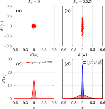
Figure 1: (a) The squeezed cloud of data points of Fourier transforms $\tilde{x}(\omega)$ in the complex plane. The parameters are $Q=65$, $F_{p}=0.025$, $\omega=1$. (b) A comparison is made between the numerical and analytical (first-order approximation) results. The fitting Gaussian distributions have zero mean and the dispersions are given by Eq. (15) for the $\tilde{x}^{\prime}(\omega)$ data points and by Eq. (17) for the $\tilde{x}^{\prime\prime}(\omega)$ data points.

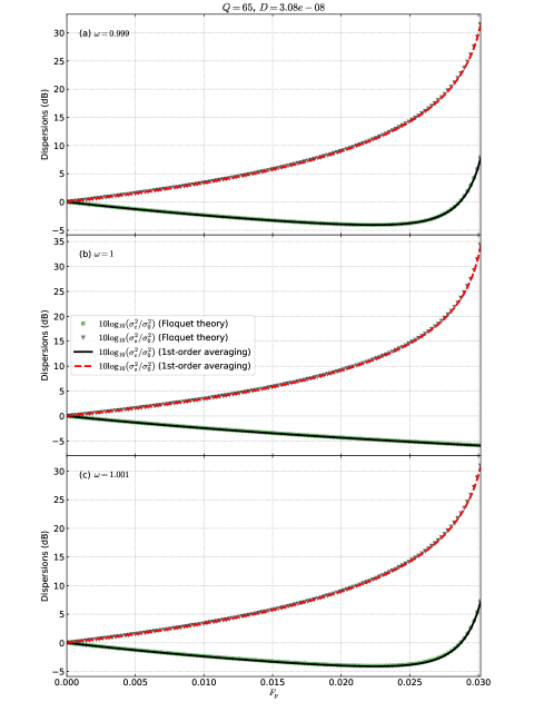
Figure 2: Comparison of the analytical (first-order averaging) standard deviations in decibels relative to the equilibrium value with zero pump of the real and imaginary parts of $\tilde{x}(\omega)$ with the corresponding Floquet theory result. (a) At $\omega=0.999$, as the pump amplitude $F_{p}$ is increased up to the instability threshold, one of the quadratures is squeezed down to a minimum above $-6~{}$dB and then it starts growing again. (b) At $\omega=1$ one sees that when the pump amplitude $F_{p}$ is increased up to the instability threshold one of the quadratures is squeezed down to $-6$ dB in amplitude while the other quadrature increases without bounds. (c) At $\omega=1.001$ one sees basically the same behavior as in frame (a).

Figure 3: Comparison of the analytical (first-order averaging) standard deviations in decibels relative to the equilibrium value with zero pump of the diagonalized dispersions (in the frame with no correlation) with the corresponding Floquet theory result. In frames (a)-(d), the $-6$ dB squeezing limit (at the bottom axes) can be reached near the instability threshold (depicted by the vertical dashed lines) even with detuning. The results for squeezing in frames (b) and (c) are in marked contrast with what happens for the same parameters in Figs. 2(a) and 2(c), respectively, where correlation was not taken into account. In frames (a) and (d) the $-6$ dB limit can be reached even with a detuning 10 times larger than in frames (b) and (c).

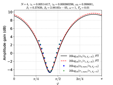
Figure 4: Gain as a function of phase for the parametrically modulated coupled resonators described in Eq. (37), with $r_{1}(t)$ replaced by $\cos(\omega t+\varphi)$ and $r_{2}(t)=0.0$. The parameters were taken from the experimental work of Singh et al. Singh et al. (2018). A comparison is made in between full numerical integration results and Floquet theory predictions of gain as a function of phase $\varphi$. The good fitting implies FT works well.

Figure 5: Floquet theory predictions for the model given in Eq. (37), with $r_{1}(t)$ replaced by $\cos(\omega t+\varphi)$ and $r_{2}(t)=0.0$. Standard deviations in decibels relative to the equilibrium value with zero pump of the diagonalized dispersions (in the frame with no correlation) obtained by Floquet theory. The dotted horizontal line represents the $-6$ dB limit and the vertical dotted line the instability threshold for each case. The common parameters used are on top of the figure. In frame (a), $\omega=0.999$, the diagonalized dispersions for each resonator are slightly off. Not much squeezing occurs up to instability threshold at the right side of the frame. In frame (b), $\omega=1$, unlike the single parametric resonator, the maximum squeezing at threshold (depicted by the vertical dashed line) is slightly above $-6$ dB. In frame (c), $\omega=1.002$, one sees that even with detuning one can reach $-6$ dB squeezing limit near the instability threshold.

IV Conclusion

Here we developed a theoretical model based on stochastic differential equations to explain the effect of white noise squeezing that occurs in classical parametrically driven resonators with added noise. This phenomenon, which is akin to the quantum phenomenon of squeezed coherent states, was first observed in a classical micromechanical resonator in 1991 by Rugar and Grütter Rugar and Grütter (1991). Unlike previous works, our results are based on the solution of stochastic differential equations both approximately, using the averaging method, and exactly, using Floquet theory. Another novelty of our model is that we obtain analytical expressions for statistical averages related to the frequency-domain response of the parametrically modulated resonator to added white noise. Each data point corresponds to a Fourier transform of a long time series with coordinates, one for each input signal in quadrature, given by the real and imaginary parts of the Fourier transform of the parametric oscillator response to the added noise. The experimental case is approximated by the ideal theoretical case in which the time constant of the LIA is infinite.

The present work is complementary to one of the authors’ (A.A.B.) previous work Batista (2012) on thermal noise squeezing. While the previous work focused on the time-domain features of squeezing, the present one focuses on the frequency domain, which is more pertinent for the LIA measurements of squeezing. Furthermore, now we also apply the theoretical tools (Floquet theory and frequency domain GFs) developed in Ref. Batista (2023) to analyze the problem.

We obtained excellent agreement between the predictions of the 1st-order averaging approximations and Floquet theory near the first parametric instability when $\omega\approx 1$ (in our dimensionless units). The strongest squeezing occurs at $\omega=1$ and when $F_{p}$ is set at the threshold of parametric instability. While in one of the quadratures fluctuations are decreased as the pumping amplitude increases, reaching a $-6$ dB deamplification in amplitude at the parametric instability threshold, in the other quadrature, fluctuations can increase without bounds. We showed that, unlike previously implied in the literature, squeezing does not quickly disappear with increasing (red or blue) detuning. We reached this conclusion by taking into account the effect of correlation, what to the best of our knowledge, had not been properly investigated in the literature. We believe this discovery could be relevant for the experimentalists. It is important to point out that the noise squeezing effect increases when one nears the parametric instability threshold, as can be seen in Eq. (17). We showed here that this is a feature of amplification near a period-doubling bifurcation point. It could be a generic feature of local codimension-1 bifurcation points and could occur in physical systems such as the Josephson junction amplifier Yamamoto et al. (2008); Vijay et al. (2009).

The present work can be extended in several ways. The methods developed here could be applied to investigate quadrature squeezing in nonlinear parametrically pumped resonators and oscillators with added noise. This could be verified experimentally in nanomechanical resonators. Also, more interestingly, since the quantum limit of these resonators has been studied in the last 10-15 years O’Connell et al. (2010); Samanta et al. (2023), one could investigate what the quadrature squeezing would be in those systems. Another system of interest is the Kerr parametric oscillator which has been implemented in superconducting circuits based on Josephson junctions Goto (2019); Grimm et al. (2020). This system is the quantum equivalent of a parametrically pumped Duffing oscillator Batista and Lisboa de Souza (2020). One simple system, but an important one, where squeezing is very relevant is the ion trap, where the stabilization is provided by parametric modulation such as occurs in Paul and Penning traps Natarajan et al. (1995). This is qualitatively very different from the sub-threshold thermal squeezing proposed by Rugar and Grütter, since there is no thermal equilibrium NSD to compare with, because in the no pumping limit the fixed point is an unstable saddle point and no oscillations occur around them.

Finally, we point out that we showed that our squeezing model based on Green’s functions and Floquet theory can be applied to coupled parametrically modulated resonators and point out that it can be further applied to any number of coupled resonators with parametric modulation and added noise with a minimum of adaptation. We believe that two- or multi-mode squeezing, where deep squeezing occurs, such as was observed with the need of feedback Poot et al. (2015); Patil et al. (2015); Sonar et al. (2018), could be found upon a more careful search of parameter space and that could be used as a guide to experimentalists.

Supplementary Material

The code used to generate all the numerical data and the figures of this paper is provided in the supplementary material.

Appendix

IV.1 The Gaussian distribution with two variables

Given the Gaussian bivariate probability distribution of the type

$$P(x,y)=\frac{\sqrt{ab-c^{2}}}{\pi}\,e^{-ax^{2}-by^{2}-2cxy},$$ (A1)

where $a,b>0$ and $ab>c^{2}$, we find $\langle x\rangle=\langle y\rangle=0$ and

$$\langle x^{2}\rangle =\frac{b}{2(ab-c^{2})},$$ (A2)

$$\langle y^{2}\rangle =\frac{a}{2(ab-c^{2})},$$

$$\langle xy\rangle =-\frac{c}{2(ab-c^{2})}.$$

Inverting these equations, we obtain all the parameters of this distribution

$$a =\frac{\langle y^{2}\rangle}{2\left(\langle x^{2}\rangle\langle y^{2}\rangle-\langle xy\rangle^{2}\right)},$$ (A3)

$$b =\frac{\langle x^{2}\rangle}{2\left(\langle x^{2}\rangle\langle y^{2}\rangle-\langle xy\rangle^{2}\right)},$$

$$c =-\frac{\langle xy\rangle}{2\left(\langle x^{2}\rangle\langle y^{2}\rangle-\langle xy\rangle^{2}\right)}.$$

Consequently, once we have the experimental data we can find the statistical averages $\langle x^{2}\rangle$, $\langle y^{2}\rangle$, and $\langle xy\rangle$, and from there obtain the probability distribution. We can also diagonalize the bilinear form at the exponent of the probability distribution. In other words we want to split the joint probability distribution into the product of two one variate distributions, that is $P(x,y)=P(u,v)=P_{-}(u)P_{+}(v)$ such that $ax^{2}+by^{2}+2cxy=\lambda_{-}u^{2}+\lambda_{+}v^{2}$. To achieve that, we diagonalize the following matrix

$$A=\left[\begin{array}[]{cc}a&c\\ c&b\end{array}\right].$$ (A4)

The characteristic equation is $\lambda^{2}-\mbox{Tr~{}}A\lambda+\mbox{det\,}A=0$, from where we obtain the eigenvalues

$$\lambda_{\pm} =\frac{\mbox{Tr~{}}A\pm\sqrt{\mbox{Tr~{}}A^{2}-4\mbox{det\,}A}}{2}=\frac{a+b\pm\sqrt{(a-b)^{2}+4c^{2}}}{2}$$ (A5)

$$=\frac{\langle x^{2}\rangle+\langle y^{2}\rangle\pm\sqrt{\left(\langle x^{2}\rangle-\langle y^{2}\rangle\right)^{2}+4\langle xy\rangle^{2}}}{4\left(\langle x^{2}\rangle\langle y^{2}\rangle-\langle xy\rangle^{2}\right)}.$$

The new distribution is

$$P(u,v)=\frac{\sqrt{\lambda_{-}\lambda_{+}}}{\pi}e^{-\lambda_{-}u^{2}-\lambda_{+}v^{2}}$$ (A6)

and the new dispersions are

$$\sigma_{-}^{2}=\langle u^{2}\rangle=\frac{1}{2\lambda_{-}},$$ (A7)

$$\sigma_{+}^{2}=\langle v^{2}\rangle=\frac{1}{2\lambda_{+}}.$$

The normalized eigenvectors are given by

$$v_{\pm}=\frac{1}{\sqrt{1+(\lambda_{\pm}-a)^{2}/c^{2}}}\left(\begin{array}[]{c}1\\ \frac{\lambda_{\pm}-a}{c}\end{array}\right).$$ (A8)

$$D=\left(\begin{array}[]{cc}\lambda_{-}&0\\ 0&\lambda_{+}\end{array}\right)=S^{T}AS,$$ (A9)

where

$$S=\Bigl{[}v_{-}\;\vline\;v_{+}\Bigr{]}.$$ (A10)

We then have

$$\begin{bmatrix}u\\ v\end{bmatrix}=\begin{bmatrix}v_{-}^{T}\\ ---\\ v_{+}^{T}\end{bmatrix}\begin{bmatrix}x\\ y\end{bmatrix}$$ (A11)

We can also assert that the tangent of the angle of the eigenvectors with respect to the $x$ axis is given by

$$\tan\theta_{\pm}=\frac{\lambda_{\pm}-a}{c}=\frac{b-a\pm\sqrt{(b-a)^{2}+4c^{2}}}{2c}=\frac{\langle y^{2}\rangle-\langle x^{2}\rangle\mp\sqrt{\left(\langle x^{2}\rangle-\langle y^{2}\rangle\right)^{2}+4\langle xy\rangle^{2}}}{2\langle xy\rangle}.$$ (A12)

We notice that when $a=b$, $\theta_{\pm}=\pm\pi/4$.

References

- Karabalin et al. (2009) R. B. Karabalin, P. X. Feng, and M. L. Roukes, Nano Letters 9, 3116 (2009).
- Thomas et al. (2013) O. Thomas, F. Mathieu, W. Mansfield, C. Huang, S. Trolier-Mckinstry, and L. Nicu, Appl. Phys. Lett. 102, 163504 (2013).
- Prakash et al. (2012) G. Prakash, A. Raman, J. Rhoads, and R. G. Reifenberger, Review of Scientific Instruments 83, 065109 (2012).
- He et al. (2023) S. He, N. Chen, H. Li, X. Fan, W. Dong, J. Dong, H. Zhou, X. Zhang, and J. Xu, IEEE Photonics Journal (2023).
- Castellanos-Beltran et al. (2008) M. Castellanos-Beltran, K. Irwin, G. Hilton, L. Vale, and K. Lehnert, Nature Physics 4, 929 (2008).
- B. H. Eom, P. K. Day, H. G. LeDuc, and Zmuidzinas (2012) B. H. Eom, P. K. Day, H. G. LeDuc, and J. Zmuidzinas, Nature Phys. 8, 623 (2012).
- Moreno-Moreno et al. (2006) M. Moreno-Moreno, A. Raman, J. Gomez-Herrero, and R. Reifenberger, Appl. Phys. Lett. 88, 193108 (2006).
- Paul (1990) W. Paul, Rev. of Mod. Phys. 62, 531 (1990).
- Miller et al. (2018) J. M. L. Miller, A. Ansari, D. B. Heinz, Y. Chen, I. B. Flader, D. D. Shin, L. G. Villanueva, and T. W. Kenny, Applied Physics Reviews 5 (2018), doi.org/10.1063/1.5027850.
- Lee et al. (2022) J. Lee, S. W. Shaw, and P. X.-L. Feng, Applied Physics Reviews 9 (2022).
- Szorkovszky et al. (2013) A. Szorkovszky, G. A. Brawley, A. C. Doherty, and W. P. Bowen, Phys. Rev. Lett. 110, 184301 (2013).
- Kimble et al. (2001) H. J. Kimble, Y. Levin, A. B. Matsko, K. S. Thorne, and S. P. Vyatchanin, Phys. Rev. D 65, 022002 (2001).
- Chen (2013) Y. Chen, Journal of Physics B: Atomic, Molecular and Optical Physics 46, 104001 (2013).
- Abbott et al. (2016) B. P. Abbott, R. Abbott, T. Abbott, M. Abernathy, F. Acernese, K. Ackley, C. Adams, T. Adams, P. Addesso, R. Adhikari, et al., Phys. Rev. Lett. 116, 061102 (2016).
- Rugar and Grütter (1991) D. Rugar and P. Grütter, Phys. Rev. Lett. 67, 699 (1991).
- DiFilippo et al. (1992) F. DiFilippo, V. Natarajan, K. R. Boyce, and D. E. Pritchard, Phys. Rev. Lett. 68, 2859 (1992).
- Natarajan et al. (1995) V. Natarajan, F. DiFilippo, and D. E. Pritchard, Phys. Rev. Lett. 74, 2855 (1995).
- Cleland (2005) A. N. Cleland, New Journal of Physics 7, 235 (2005).
- Mahboob et al. (2014) I. Mahboob, H. Okamoto, K. Onomitsu, and H. Yamaguchi, Phys. Rev. Lett. 113, 167203 (2014).
- Patil et al. (2015) Y. Patil, S. Chakram, L. Chang, and M. Vengalattore, Phys. Rev. Lett. 115, 017202 (2015).
- Pontin et al. (2016) A. Pontin, M. Bonaldi, A. Borrielli, L. Marconi, F. Marino, G. Pandraud, G. Prodi, P. Sarro, E. Serra, and F. Marin, Physical review letters 116, 103601 (2016).
- Singh et al. (2018) R. Singh, R. J. Nicholl, K. I. Bolotin, and S. Ghosh, Nano Letters 18, 6719 (2018).
- Zhao et al. (2021) Z. Zhao, H. Chen, W. Li, Z. Cheng, H. Song, Y. Wang, Q. Zhou, X. Niu, and G. Deng, in 2021 13th International Conference on Wireless Communications and Signal Processing (WCSP) (IEEE, 2021) pp. 1–3.
- Vinante and Falferi (2013) A. Vinante and P. Falferi, Phys. Rev. Lett. 111, 207203 (2013).
- Poot et al. (2015) M. Poot, K. Y. Fong, and H. Tang, New Journal of Physics 17, 043056 (2015).
- Sonar et al. (2018) S. Sonar, V. Fedoseev, M. J. Weaver, F. Luna, E. Vlieg, H. van der Meer, D. Bouwmeester, and W. Löffler, Physical Review A 98, 013804 (2018).
- Almog et al. (2007) R. Almog, S. Zaitsev, O. Shtempluck, and E. Buks, Phys. Rev. Lett. 98, 078103 (2007).
- Huber et al. (2020) J. S. Huber, G. Rastelli, M. J. Seitner, J. Kölbl, W. Belzig, M. I. Dykman, and E. M. Weig, Phys. Rev. X 10, 021066 (2020).
- Wiesenfeld (1985) K. Wiesenfeld, J. of Stat. Phys. 38, 1071 (1985).
- Batista (2011) A. A. Batista, J. of Stat. Mech. (Theory and Experiment) 2011, P02007 (2011).
- Batista et al. (2022) A. A. Batista, A. A. L. de Souza, and R. S. N. Moreira, Journal of Applied Physics 132, 174902 (2022).
- Batista (2012) A. A. Batista, Phys. Rev. E 86, 051107 (2012).
- J. M. L. Miller et al. (2020) J. M. L. Miller, D. D. Shin, H.-K. Kwon, S. W. Shaw, and T. W. Kenny, Appl. Phys. Lett. 117, 033504 (2020).
- Batista (2023) A. A. Batista, arXiv preprint arXiv:2306.13556v2 (2023).
- Singh et al. (2020) R. Singh, A. Sarkar, C. Guria, R. J. Nicholl, S. Chakraborty, K. I. Bolotin, and S. Ghosh, Nano Letters 20, 4659–4666 (2020).
- Yamamoto et al. (2008) T. Yamamoto, K. Inomata, M. Watanabe, K. Matsuba, T. Miyazaki, W. D. Oliver, Y. Nakamura, and J. Tsai, Applied Physics Letters 93, 042510 (2008).
- Vijay et al. (2009) R. Vijay, M. H. Devoret, and I. Siddiqi, Review of Scientific Instruments 80, 111101 (2009).
- O’Connell et al. (2010) A. D. O’Connell, M. Hofheinz, M. Ansmann, R. C. Bialczak, M. Lenander, E. Lucero, M. Neeley, D. Sank, H. Wang, M. Weides, and A. N. Cleland, Nature 464, 697 (2010).
- Samanta et al. (2023) C. Samanta, S. De Bonis, C. Møller, R. Tormo-Queralt, W. Yang, C. Urgell, B. Stamenic, B. Thibeault, Y. Jin, D. Czaplewski, et al., Nature Physics 19, 1340–1344 (2023).
- Goto (2019) H. Goto, Journal of the Physical Society of Japan 88, 061015 (2019).
- Grimm et al. (2020) A. Grimm, N. E. Frattini, S. Puri, S. O. Mundhada, S. Touzard, M. Mirrahimi, S. M. Girvin, S. Shankar, and M. H. Devoret, Nature 584, 205 (2020).
- Batista and Lisboa de Souza (2020) A. A. Batista and A. A. Lisboa de Souza, Jour. of Appl. Phys. 128, 244901 (2020).