LancBiO: Dynamic Lanczos-aided Bilevel Optimization via Krylov Subspace

Abstract

Bilevel optimization, with broad applications in machine learning, has an intricate hierarchical structure. Gradient-based methods have emerged as a common approach to large-scale bilevel problems. However, the computation of the hyper-gradient, which involves a Hessian inverse vector product, confines the efficiency and is regarded as a bottleneck. To circumvent the inverse, we construct a sequence of low-dimensional approximate Krylov subspaces with the aid of the Lanczos process. As a result, the constructed subspace is able to dynamically and incrementally approximate the Hessian inverse vector product with less effort and thus leads to a favorable estimate of the hyper-gradient. Moreover, we propose a provable subspace-based framework for bilevel problems where one central step is to solve a small-size tridiagonal linear system. To the best of our knowledge, this is the first time that subspace techniques are incorporated into bilevel optimization. This successful trial not only enjoys $\mathcal{O}(\epsilon^{-1})$ convergence rate but also demonstrates efficiency in a synthetic problem and two deep learning tasks.

1 Introduction

Bilevel optimization, in which upper-level and lower-level problems are nested with each other, mirrors a multitude of applications, e.g., game theory (Stackelberg, 1952), hyper-parameter optimization (Franceschi et al., 2017, 2018), meta-learning (Bertinetto et al., 2018), neural architecture search (Liu et al., 2018; Wang et al., 2022), adversarial training (Wang et al., 2021), reinforcement learning (Chakraborty et al., 2023; Hong et al., 2023).

In this paper, we consider the following bilevel problem:

$$\begin{array}[]{cl}\min\limits_{x\in\mathbb{R}^{d_{x}}}&\varphi(x):=f\left(x,y^{*}(x)\right)\\ \mathrm{s.\,t.}&y^{*}(x)\in\operatorname*{arg\,min}\limits_{y\in\mathbb{R}^{d_{y}}}g(x,y),\end{array}$$ (1)

where the upper-level function $f$ and the lower-level function $g$ are defined on $\mathbb{R}^{d_{x}}\times\mathbb{R}^{d_{y}}$. $\varphi$ is called the hyper-objective, and the gradient of $\varphi(x)$ is referred to as the hyper-gradient (Pedregosa, 2016; Grazzi et al., 2020; Chen et al., 2023; Yang et al., 2023) if it exists. In contrast to standard single-level optimization problems, bilevel optimization is inherently challenging due to its intertwined structure. Specifically, the formulation (1) underscores the crucial role of the lower-level solution $y^{*}(x)$ in each update of $x$.

One of the focal points in recent bilevel methods has shifted towards nonconvex upper-level problems coupled with strongly convex lower-level problems (Ghadimi & Wang, 2018; Ji et al., 2021; Chen et al., 2022; Dagréou et al., 2022; Li et al., 2022; Hong et al., 2023). This configuration ensures that $y^{*}(x)$ is a single-valued function of $x$, i.e., $y^{*}(x)=\operatorname*{arg\,min}_{y\in\mathbb{R}^{d_{y}}}g(x,y)$. Subsequently, the hyper-gradient can be computed from the implicit function theorem as follows (Ghadimi & Wang, 2018),

$$\nabla\varphi(x)= ~{}\nabla_{x}f\left(x,y^{*}\left(x\right)\right)-\nabla^{2}_{xy}g\left(x,y^{*}\left(x\right)\right)$$ (2)

$$\times\left[\nabla_{yy}^{2}g\left(x,y^{*}\left(x\right)\right)\right]^{-1}\nabla_{y}f\left(x,y^{*}\left(x\right)\right).$$

The gradient methods based on the hyper-gradient, $x_{k+1}=x_{k}-\lambda\nabla\varphi(x_{k}),$ are known as the approximate implicit differentiation (AID) based methods (Ji et al., 2021; Arbel & Mairal, 2022; Liu et al., 2023). Nevertheless, the computation of the hyper-gradient (2) suffers from two pains: 1) solving the lower-level problem to obtain $y^{*}(x)$; 2) assembling the Hessian inverse vector product

$$v^{*}(x):=\left[\nabla_{yy}^{2}g\left(x,y^{*}\left(x\right)\right)\right]^{-1}\nabla_{y}f\left(x,y^{*}\left(x\right)\right),$$ (3)

or equivalently, solving a large linear system in terms of $v$,

$$\nabla^{2}_{yy}g(x,y^{*}(x))v=\nabla_{y}f(x,y^{*}(x)).$$ (4)

To this end, it is beneficial to adopt a few inner iterations to approximate $y^{*}(x)$ and $v^{*}(x)$ within each outer iteration (i.e., the update of $x$). Note that the approximation accuracy of $v^{*}(x)$ is crucial for the AID-based methods; see (Ji et al., 2022; Li et al., 2022). Specifically, Figure 1 confirms that the more inner iterations, the higher quality of the estimate of $v^{*}$, and the more enhanced descent of the objective function within the same number of outer iterations..

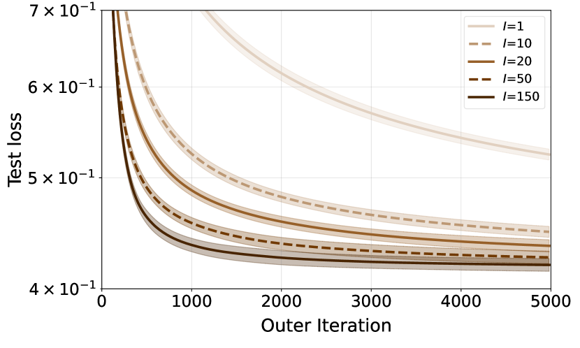
Figure 1: Test loss for the method stocBiO (Ji et al., 2021) with different inner iterations $I$ to approximate the Hessian inverse vector product.

Approximation: Existing efforts are dedicated to approximating $v^{*}$ in different fashions by regulating the number of inner iterations, e.g., the Neumann series approximation (Ghadimi & Wang, 2018; Ji et al., 2021) for the inverse, gradient descent (Arbel & Mairal, 2022; Dagréou et al., 2022) and conjugate gradient descent (Pedregosa, 2016; Yang et al., 2023) for the linear system.

Amortization: Moreover, there are studies aimed at amortizing the cost of approximation through outer iterations. These methods include using the inner estimate from the previous outer iteration as a warm start for the current outer iteration (Ji et al., 2021; Arbel & Mairal, 2022; Dagréou et al., 2022; Ji et al., 2022; Li et al., 2022; Xiao et al., 2023), or employing a refined step size control (Hong et al., 2023).

Subspace techniques, widely adopted in nonlinear optimization (Yuan, 2014), approximately solve large-scale problems in lower-dimensional subspaces, which not only reduce the computational cost significantly but also enjoy favorable theoretical properties as in full space models. Taking into account the above two principles, it is reasonable to consider subspace techniques in bilevel optimization. Specifically, we can efficiently amortize the construction of low-dimensional subspaces and sequentially solve linear systems (4) in these subspaces to approximate $v^{*}$ accurately.

1.1 Contributions

In this paper, taking advantage of the Krylov subspace and the Lanczos process, we develop an innovative subspace-based framework—LancBiO, which features an efficient and accurate approximation of the Hessian inverse vector product $v^{*}$ in the hyper-gradient—for bilevel optimization. The main contributions are summarized as follows.

Firstly, we build up a dynamic process for constructing low-dimensional subspaces that are tailored from the Krylov subspace for bilevel optimization. This process effectively reduces the large-scale subproblem (4) to the small-size tridiagonal linear system, which draws on the spirit of the Lanczos process. To the best of our knowledge, this is the first time that the subspace technique is leveraged in bilevel optimization.

Moreover, the constructed subspaces enable us to dynamically and incrementally approximate $v^{*}$ across outer iterations, thereby achieving an enhanced estimate of the hyper-gradient; Figure 2 illustrates that the proposed LancBiO reaches the best estimation error for $v^{*}$. Hence, we provide a new perspective for approximating the Hessian inverse vector product in bilevel optimization. Specifically, the number of Hessian-vector products averages at $(1+\frac{1}{m})$ per outer iteration with the subspace dimension $m$, which is favorably comparable with the existing methods.

​​​​​​​​​​

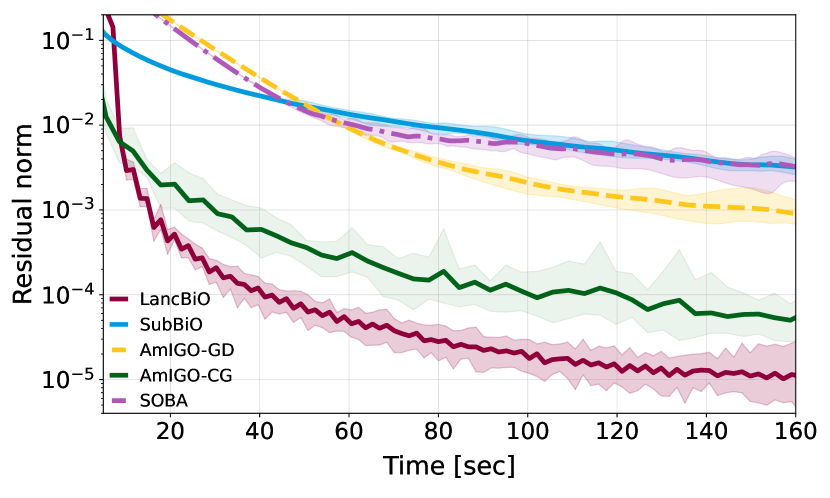
Figure 2: Estimation error of the Hessian inverse vector product in hyper-data cleaning task with corruption rate $0.5$ for different methods: LancBiO and SubBiO (ours), AmIGO (Arbel & Mairal, 2022), and SOBA (Dagréou et al., 2022).

Finally, we offer analysis to circumvent the instability in the process of approximating subspaces, with the result that LancBiO can profit from the benign properties of the Krylov subspace. We prove that the proposed method LancBiO is globally convergent with the convergence rate $\mathcal{O}(\epsilon^{-1})$. In addition, the efficiency of LancBiO is validated by a synthetic problem and two deep learning tasks.

1.2 Related Work

A detailed introduction to bilevel optimization methods can be found in Appendix A.

Krylov subspace methods: Subspace techniques have gained significant recognition in the realm of numerical linear algebra (Parlett, 1998; Saad, 2011; Golub & Van Loan, 2013) and nonlinear optimization (Yuan, 2014; Liu et al., 2021). Specifically, numerous optimization methods utilized subspace techniques to improve efficiency, including acceleration technique (Li et al., 2020), diagonal preconditioning (Gao et al., 2023), and derivative-free optimization methods (Cartis & Roberts, 2023). Krylov subspace (Krylov, 1931), due to its special structure,

$$\mathcal{K}_{N}(A,b):=\operatorname{span}\left\{b,Ab,A^{2}b,\ldots,A^{N-1}b\right\}$$

with the dimension $N$ for a matrix $A$ and a vector $b$, exhibits advantageous properties in convex quadratic optimization (Nesterov et al., 2018), eigenvalue computation (Kuczyński & Woźniakowski, 1992), and regularized nonconvex quadratic problems (Carmon & Duchi, 2018). Krylov subspace has been widely considered in large-scale optimization such as trust region methods (Gould et al., 1999), trace maximization problems (Liu et al., 2013), and cubic Newton methods (Cartis et al., 2011; Jiang et al., 2024). Lanczos process (Lanczos, 1950) is an orthogonal projection method onto the Krylov subspace, which reduces a dense symmetric matrix to a tridiagonal form. Details of the Krylov subspace and the Lanczos process are summarized in Appendix B.

Approximation of the Hessian inverse vector product : It is cumbersome to compute the Hessian inverse vector product in bilevel optimization. To bypass it, several strategies implemented through inner iterations were proposed, e.g., the Neumann series approximation (Ghadimi & Wang, 2018; Ji et al., 2021), gradient descent (Arbel & Mairal, 2022; Dagréou et al., 2022), and conjugate gradient descent (Pedregosa, 2016; Arbel & Mairal, 2022; Yang et al., 2023). Alternatively, the previous information was exploited in (Ji et al., 2021; Arbel & Mairal, 2022) as a warm start for outer iterations; Ramzi et al. (2022) suggested approximating the Hessian inverse in the manner of quasi-Newton; Dagréou et al. (2022) and Li et al. (2022) proposed the frameworks without inner iterations to approximate the Hessian inverse vector product.

2 Subspace-based Algorithms

In this section, we dive into the development of bilevel optimization algorithms for solving (1), which dynamically construct subspaces to approximate the Hessian inverse vector product.

The (hyper-)gradient descent method carries out the $k$-th outer iteration as follows,

$$x_{k+1}=x_{k}-\lambda\nabla\varphi(x_{k}),$$

where the hyper-gradient is exactly computed by

$$\nabla\varphi(x_{k})=\nabla_{x}f\left(x_{k},y^{*}_{k}\right)-\nabla^{2}_{xy}g\left(x_{k},y^{*}_{k}\right)v^{*}_{k}$$

with $y^{*}_{k}:=y^{*}(x_{k})$ and $v^{*}_{k}:=v^{*}(x_{k})$ defined in (3). In view of the computational intricacy of $y^{*}_{k}$ and $v^{*}_{k}$, it is commonly concerned with the following estimator for the hyper-gradient

$$\widetilde{\nabla}\varphi\left(x_{k},y_{k},v_{k}\right):=\nabla_{x}f\left(x_{k},y_{k}\right)-\nabla^{2}_{xy}g\left(x_{k},y_{k}\right)v_{k},$$ (5)

where $y_{k}$ is an approximation of $y^{*}_{k}$. Denote the Hessian

$$A_{k}=\nabla_{yy}^{2}g(x_{k},y_{k})\quad\text{and}\quad b_{k}=\nabla_{y}f(x_{k},y_{k}).$$

$v_{k}$ is the (approximate) solution of a quadratic optimization problem

$$\min_{v\in\mathcal{S}_{k}}\frac{1}{2}v^{\top}A_{k}v-v^{\top}b_{k},$$ (6)

where $\mathcal{S}_{k}$ is the full space $\mathbb{R}^{d_{y}}$ and the exact solution is $A_{k}^{-1}b_{k}$. Subsequently, in order to reduce the computational cost, it is natural to ask:

Can we construct a low-dimensional subspace $\mathcal{S}_{k}$ such that the solution of (6) satisfactorily approximates $A_{k}^{-1}b_{k}$?

General subspace constructions introduced in the existing subspace methods (Yuan, 2014; Liu et al., 2021) are not straightforward and not exploited in the bilevel setting, rendering the exploration of appropriate subspaces challenging. In the following subsections, we construct approximate Krylov subspaces and propose an elaborate subspace-based framework for bilevel problems.

2.1 Why Krylov subspace: the SubBiO algorithm

In light of the Neumann series for a suitable $\eta\in\mathbb{R}$

$$A^{-1}b=\eta\sum_{i=0}^{\infty}(I-\eta A)^{i}b,$$ (7)

it is observed from Appendix B that $A^{-1}b$ belongs to a Krylov subspace for some $N>0$, i.e.,

$$A^{-1}b\in\mathcal{K}_{N}(A,b)=\mathcal{K}_{N}(I-\eta A,b).$$

Hence, it is reasonable to consider a Krylov subspace for the construction of $\mathcal{S}_{k}$.

Given a constant $n\ll N$, we consider an approximation of $A^{-1}b$ in a lower-dimensional Krylov subspace $\mathcal{K}_{n}(A,b)$, i.e., $v_{n}\in\mathcal{K}_{n}(A,b)=\mathcal{K}_{n}(I-\eta A,b)$ and

$$v_{n}=\sum_{i=0}^{n-1}{c_{i}\left(I-\eta A\right)^{i}b}\approx A^{-1}b.$$

Note that the approximation $v_{n}$ is composed of the set $\{\left(I-\eta A\right)^{i}b\}_{i=0}^{n-1}$ in the sense of the Neumann series (7). Moreover, we observe that $(I-\eta A)v_{n}\in\mathcal{K}_{n+1}(A,b)$ and hence we can recursively choose

$$v_{n+1}\in\mathcal{S}_{n+1}:=\operatorname{span}\left\{b,(I-\eta A)v_{n}\right\}\subseteq\mathcal{K}_{{n+1}}(A,b)$$

since the subspace $\operatorname{span}\left\{b,(I-\eta A)v_{n}\right\}$ includes the information of the increased set $\{\left(I-\eta A\right)^{i}b\}_{i=0}^{n}$. In summary, we can construct a sequence of two-dimensional subspaces $\{\mathcal{S}_{n}\}$ that implicitly filters information from the Krylov subspaces. The rationale for this procedure can be illustrated in Figure 3.

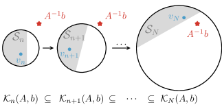
Figure 3: Illustration of approximating $A^{-1}b\in\mathcal{K}_{{N}}(A,b)$ by $v_{n}$ in the two-dimensional subspace $\mathcal{S}_{n}\subseteq\mathcal{K}_{{n}}(A,b)$.

In the context of bilevel optimization, we seek the best solution $v_{k}$ to the subproblem (6) in the subspace

$$\mathcal{S}_{k}=\operatorname{span}\left\{b_{{k}},(I-\eta A_{{k}})v_{k-1}\right\}.$$ (8)

Repeating the procedure is capable of dynamically approximating the Hessian inverse vector product, i.e., $v_{k}$ approximates $A_{k}^{-1}b_{k}$. The Krylov Subspace-aided Bilevel Optimization algorithm (SubBiO) is listed in Algorithm 1.

Algorithm 1 SubBiO

0:  iteration threshold $K$, step sizes $\theta,\lambda,\eta$, initialization $x_{1},y_{1},v_{0}$

1:  for $k=1,2,\dots,K$ do

2:     $A_{k}=\nabla_{yy}^{2}g\left(x_{k},y_{k}\right)$, $b_{k}=\nabla_{y}f(x_{k},y_{k})$

3:     ${\mathcal{S}_{k}=\operatorname{span}\{b_{k},\left(I-\eta A_{k}\right)v_{k-1}\}}$

4:     $v_{k}=\operatorname*{arg\,min}_{v\in{\mathcal{S}_{k}}}\frac{1}{2}v^{\top}A_{k}v-b_{k}^{\top}v$

5:     $x_{k+1}=x_{k}-\lambda\left(\nabla_{x}f(x_{k},y_{k})-\nabla^{2}_{xy}g(x_{k},y_{k})v_{k}\right)$

6:     $y_{k+1}=y_{k}-\theta\nabla_{y}g(x_{k+1},y_{k})$

7:  end for

7:  $(x_{K+1},y_{K+1})$

2.2 Why dynamic Lanczos: the LancBiO framework

Notice that the subproblem in SubBiO (Algorithm 1) can be equivalently reduced to

$$\min_{z\in\mathbb{R}^{2}}\frac{1}{2}z^{\top}(S_{k}^{\top}A_{k}S_{k})z-b_{k}^{\top}S_{k}z,$$

where $S_{k}:=[b_{k}\,\,\left(I-\eta A_{k}\right)v_{k-1}]\in\mathbb{R}^{d_{y}\times 2}$. The solution $z^{*}\in\mathbb{R}^{2}$ results in $v_{k}=S_{k}z^{*}$. It is a two-dimensional subproblem, whereas computing the projection $S_{k}^{\top}A_{k}S_{k}$ requires two Hessian-vector products, which dominate the cost of the subproblem. Therefore, it is crucial to reduce or amortize the projection cost while preserving the advantages of the Krylov subspace. To this end, we find that the Lanczos process (Appendix B) provides an enlightening way (Lanczos, 1950; Saad, 2011; Golub & Van Loan, 2013) since it allows for the construction of a Krylov subspace and maintaining a tridiagonal matrix as the projection matrix, which significantly reduces the computational cost.

In bilevel optimization, since the quadratic problem (6) evolves through outer iterations, it is difficult to leverage the Lanczos process to amortize the projection cost while simultaneously updating variables as in SubBiO. Specifically, the Lanczos process is inherently unstable (Paige, 1980), and thus the accumulative difference among $\{A_{k}\}$ and $\{b_{k}\}$ will make the Lanczos process invalid.

In order to address the above difficulties, we propose a restart mechanism to guarantee the benign behavior of approximating the Krylov subspace and consider solving residual systems to employ the historical information. In summary, we propose a dynamic Lanczos-aided Bilevel Optimization framework, LancBiO, which is listed in Algorithm 2. The only difference between LancBiO and SubBio is solving the subproblem (line 3-4 in Algorithm 1).

Algorithm 2 LancBiO

0:  iteration threshold $K$, step sizes $\theta,\lambda$, initialization $x_{1},y_{1},v_{1}$, initial correction $\Delta v_{0}=0$, subspace dimension $m$, initial epoch $h=-1$

1:  for $k=1,2,\dots,K$ do

2:     $A_{k}=\nabla^{2}_{yy}g(x_{k},y_{k}),\ b_{k}=\nabla_{y}f(x_{k},y_{k})$

3:     if $(k\ \texttt{mod}\ m)=1$ then

4:        $h=h+1$

5:        $\bar{v}_{h}=v_{k}$

6:        $w_{h}=A_{k}\bar{v}_{h}$

7:        $Q_{k-1}=(b_{k}-w_{h})/\left\|{b_{k}-w_{h}}\right\|$

8:        $T_{k-1}=\texttt{Empty Matrix}$

9:        $\beta_{k}=0$

10:     end if

11:     $(T_{k},Q_{k},\beta_{k+1})\!=\!\texttt{DLanczos}(T_{k-1},Q_{k-1},A_{k},\beta_{k})$

12:     $r_{k}=b_{k}-w_{h}$

13:     $\Delta v_{k}=Q_{k}(T_{k})^{-1}Q_{k}^{\top}r_{k}$

14:     $v_{k}=\bar{v}_{h}+\Delta v_{k}$

15:     $x_{k+1}=x_{k}-\lambda\left(\nabla_{x}f(x_{k},y_{k})-\nabla^{2}_{xy}g(x_{k},y_{k})v_{k}\right)$

16:     $y_{k+1}=y_{k}-\theta\nabla_{y}g(x_{k+1},y_{k})$

17:  end for

17:  $(x_{K+1},\ y_{K+1})$

If we adapt the standard Lanczos process for tridiagonalizing $A_{k}$, by starting from $q_{1}=b_{1}/\left\|{b_{1}}\right\|,\ q_{0}={\bf 0},\ \beta_{1}=0$ and using the dynamic matrices $A_{j}$ for $j=1,2,\ldots,k$, the process is as follows,

$$u_{j} =A_{j}q_{j}-\beta_{j}q_{j-1},$$

$$\alpha_{j} =q_{j}^{\top}u_{j},$$

$$\omega_{j} =u_{j}-\alpha_{j}q_{j},$$

$$\beta_{j+1} =\left\|\omega_{j}\right\|,$$

$$q_{j+1} =\omega_{j}/\beta_{j+1},$$

and $T_{k}$ is a tridiagonal matrix recursively computed from

Restart mechanism: In contrast to SubBiO, we construct the subspace

$$\mathcal{S}_{k}=\operatorname{span}(Q_{k})=\operatorname{span}([q_{1},\ldots,q_{k}]).$$

Consequently, $Q_{k}$ approximates the basis of the true Krylov subspace $\mathcal{K}_{k}(A_{k},b_{k})$, and $T_{k}$ approximates the projection of $A_{k}$ onto it, i.e.,

$$T_{k}\approx Q_{k}^{\top}A_{k}Q_{k}.$$

However, $Q_{k}$ will lose the orthogonality due to the evolution of $A_{j}$, and $T_{k}$ will deviate from the true projection. Based on this observation, we restart the subspace spanned by the matrix $Q$ for every $m$ outer iterations (line 3 to line 10 in Algorithm 2). The restart mechanism allows us to mitigate the accumulation of the difference among $\{A_{1},\dots,A_{k}\}$, and hence, we can maintain a more reliable basis matrix to approximate Krylov subspaces. The above dynamic Lanczos subroutine, DLanczos, is summarized in Appendix C (line 11 in Algorithm 2).

Residual minimization: The preceding discussion reveals that the dimension of the subspace $\mathcal{S}_{k}$ should be moderate to retain the reliability of the dynamic process. Nevertheless, the limited dimension stagnates the approximation of the subproblem (6) to the full space problem. Therefore, instead of solving the quadratic subproblem (6) in the subspace, we intend to find $v\in\mathcal{S}_{k}=\operatorname{span}(Q_{k})$ such that $A_{k}v\approx b_{k}$. To this end, after going through $m$ outer iterations, we denote the current approximation by $\bar{v}$. In the subsequent outer iterations, we concentrate on a linear system with a residual in the form

$$A_{k}\Delta v=b_{k}-A_{k}\bar{v},\quad\quad\Delta v\in\mathcal{S}_{k}.$$ (9)

Specifically, we inexactly solve the minimal residual subproblem

$$\min_{\Delta v\in\mathcal{S}_{k}}\left\|{(b_{k}-A_{k}\bar{v})-A_{k}\Delta v}\right\|^{2}$$ (10)

and use the solution $\Delta v_{k}$ as a correction to $\bar{v}$ (line 12 to line 14 in Algorithm 2),

$$v_{k}=\bar{v}+\Delta v_{k}.$$

Consequently, taking into account the two strategies above, we illuminate the framework LancBiO in Figure 4. It is structured into epochs, with each epoch built by $m$ outer iterations. Notably, each epoch restarts by incrementally constructing from a one-dimensional space $Q_{1}$ to an $m$-dimensional space $Q_{m}$, aiming to approximate the solution to the residual system within these subspaces. The solution $\Delta v_{j}$ to the subproblem serves as a correction to enhance the hyper-gradient estimation, which facilitates the $(x,y)$ updating.

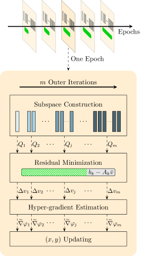
Figure 4: An overview of LancBiO.

The combination of the two strategies, restart mechanism and residual minimization, not only controls the dimension of the subspace but also utilizes historical information to enhance the approximation accuracy. By considering a simplified scenario, we reduce the two strategies into solving a standard linear system problem $Ax=b$ with $A$ and $b$ fixed. Note that, from the perspective of Theorem 1 in (Carmon & Duchi, 2018), the residual associated with solving a linear system in an $m$-dimensional Krylov subspace decays faster than a rate $\mathcal{O}\left({{1}/{m^{2}}}\right)$ after each restart. In other words, the estimation error of the Hessian inverse vector product experiences a decay rate of $\mathcal{O}\left({{1}/{m^{2}}}\right)$ after every restart, i.e.,

$$\frac{\left\|b-Av_{m\left(h+1\right)}\right\|}{\left\|b-Av_{mh}\right\|}=\frac{\left\|\left(b-A\bar{v}_{h}\right)-A\Delta_{m\left(h+1\right)}\right\|}{\left\|b-A\bar{v}_{h}\right\|}=\mathcal{O}\left(\frac{1}{m^{2}}\right).$$

Remark 2.1.

The classic Lanczos process is known for its capability to solve indefinite linear systems (Greenbaum et al., 1999). In the same fashion, the LancBiO framework can be adapted to the bilevel problems with a nonconvex lower-level problem. Interested readers are referred to Appendix D for more details.

2.3 Relation to the existing algorithms

The proposed SubBiO and LancBiO have intrinsic connections to the existing algorithms. Generally, in each outer iteration, methods such as BSA (Ghadimi & Wang, 2018) and TTSA (Hong et al., 2023) truncate the Neumann series (7) at $N$, exploiting information from an $N$-dimensional Krylov subspace. On the contrary, both SubBiO and LancBiO implicitly gather knowledge from a high-dimensional Krylov subspace with less effort.

SubBiO shares similarities with SOBA (Dagréou et al., 2022) and FSLA (Li et al., 2022). The update rule for the estimator $v$ of the Hessian inverse vector product in SOBA and FSLA is

$$v_{k} =v_{k-1}-\eta\left(A_{k}v_{k-1}-b_{k}\right)$$

$$=(I-\eta A_{k})v_{k-1}+\eta b_{k},$$

while the proposed SubBiO constructs a two-dimensional subspace, $\mathcal{S}_{k}=\operatorname{span}\left\{b_{{k}},(I-\eta A_{{k}})v_{k-1}\right\}$, defined in (8). It is worth noting that the updated $v_{k}$ in SOBA and FSLA belongs to the subspace $\mathcal{S}_{k}$. Furthermore, in the sense of solving the two-dimensional subproblem (6), SubBiO selects the optimal solution $v$ in the subspace.

In addition, if the subspace dimension $m$ is set to one, LancBiO is simplified to a scenario in which one conjugate gradient (CG) step with the warm start mechanism is performed in each outer iteration, which exactly recovers the algorithm AmIGO-CG (Arbel & Mairal, 2022) with one inner iteration to the update of $v$. Alternatively, if the step size $\lambda$ in Algorithm 2 is set to $0$ within each $m$-steps (i.e., only inner iterations are invoked), LancBiO reduces to the algorithm AmIGO-CG (Arbel & Mairal, 2022) with $m$ inner iterations.

3 Theoretical Analysis

In this section, we provide a non-asymptotic convergence analysis for LancBiO. Firstly, we introduce some appropriate assumptions. Subsequently, to address the principal theoretical challenges, we analyze the properties and dynamics of the subspaces constructed in Section 2. Finally, we prove the global convergence of LancBiO and give the iteration complexity; the detailed proofs are provided in the appendices.

Assumption 3.1.

The upper-level function $f$ is twice continuously differentiable. The gradients $\nabla_{x}f(x,y)$ and $\nabla_{y}f(x,y)$ are $L_{fx}$-Lipschitz and $L_{fy}$-Lipschitz, and $\left\|{\nabla_{y}f\left({x,y^{*}(x)}\right)}\right\|\leq C_{fy}$.

Assumption 3.2.

The lower-level function $g$ is twice continuously differentiable. $\nabla_{x}g(x,y)$ and $\nabla_{y}g(x,y)$ are $L_{gx}$-Lipschitz and $L_{gy}$-Lipschitz. The derivative $\nabla^{2}_{xy}g(x,y)$ and the Hessian matrix $\nabla^{2}_{yy}g(x,y)$ are $L_{gxy}$-Lipschitz and $L_{gyy}$-Lipschitz.

Assumption 3.3.

For any $x\in\mathbb{R}^{d_{x}}$, the lower-level function $g(x,\cdot)$ is $\mu_{g}$-strongly convex.

The Lipschitz properties of $f,g$ and the strong convexity of the lower-level problem revealed by the above assumptions are standard in bilevel optimization (Ghadimi & Wang, 2018; Chen et al., 2021; Ji et al., 2021; Khanduri et al., 2021; Arbel & Mairal, 2022; Chen et al., 2022; Dagréou et al., 2022; Li et al., 2022; Ji et al., 2022; Hong et al., 2023). These assumptions ensure the smoothness of $\varphi$ and $y^{*}$; see the following results (Ghadimi & Wang, 2018).

Lemma 3.4.

Under the Assumptions 3.2 and 3.3, $y^{*}(x)$ is ${L_{gx}}/{\mu_{g}}$ -Lipschitz continuous, i.e., for any $x_{1},x_{2}\in\mathbb{R}^{d_{x}}$,

$$\left\|{y^{*}(x_{1})-y^{*}(x_{2})}\right\|\leq\frac{L_{gx}}{\mu_{g}}\left\|{x_{1}-x_{2}}\right\|.$$ (11)

Lemma 3.5.

Under the Assumptions 3.1, 3.2 and 3.3, the hyper-gradient $\nabla\varphi(\cdot)$ is $L_{\varphi}$-Lipschitz continuous, i.e., for any $x_{1},x_{2}\in\mathbb{R}^{d_{x}}$,

$$\left\|{\nabla\varphi(x_{1})-\nabla\varphi(x_{2})}\right\|\leq L_{\varphi}\left\|{x_{1}-x_{2}}\right\|,$$

where $L_{\varphi}>0$ is defined in Appendix E.

Assumption 3.6.

There exists a constant $C_{fx}$ so that $\left\|{\nabla_{x}f(x,y)}\right\|\leq C_{fx}$.

3.6, commonly adopted in (Ghadimi & Wang, 2018; Ji et al., 2021; Liu et al., 2022; Kwon et al., 2023b), is helpful in ensuring the stable behavior of the dynamic Lanczos process; see Section 3.1.

3.1 Subspace Properties in Dynamic Lanczos Process

In view of the inherent instability of the Lanczos process (Paige, 1980; Meurant & Strakoš, 2006) and the evolution of the Hessian $\{A_{k}\}$ and the gradient $\{b_{k}\}$ in LancBiO, the analysis of the constructed subspaces is intricate. Based on the existing work (Paige, 1976, 1980; Greenbaum, 1997), this subsection sheds light on the characterization of subspaces and the effectiveness of the subproblem in approximating the full space problem in LancBiO.

An epoch is constituted of a complete $m$-step dynamic Lanczos process between two restarts, namely, after $h$ epochs, the number of outer iterations is $mh$. Given the outer iterations $k=mh+j$ for $j=1,2,\ldots,m$, we denote

$$\varepsilon_{st}^{h}:=\left(1+\frac{L_{gx}}{\mu_{g}}\right)\left\|x_{mh+s}-x_{mh+t}\right\|+\left\|y_{mh+s}-y_{mh+s}^{*}\right\|$$

for $s,t=1,2,\dots,m$ and

$$\varepsilon_{j}^{h}:=\max_{1\leq s,t\leq j}\varepsilon_{st}^{h},$$

serving as the accumulative difference. For brevity, we omit the superscript where there is no ambiguity, and we are slightly abusing of notation that at the current epoch, $\{A_{mh+j}\}$ and $\{b_{mh+j}\}$ are simplified by $\{A_{j}\}$ and $\{b_{j}\}$ for $j=1,\dots,m$. In addition, the approximations in the residual system (9) are simplified by $\bar{v}$ and $\bar{b}:=b_{1}-A_{1}\bar{v}$.

The following proposition characterizes that the dynamic subspace constructed in Algorithm 2 within an epoch is indeed an approximate Krylov subspace.

Proposition 3.7.

At the $j$-th step within an epoch ($j=1,2,\ldots,m-1$), the subspace spanned by the matrix $Q_{j+1}$ in Algorithm 2 satisfies

$$\mathrm{span}(Q_{j+1})\subseteq\mathrm{span}\left\{A_{1}^{a_{1}}A_{2}^{a_{2}}\cdots A_{j}^{a_{j}}\bar{b}\,\left|\!\begin{array}[]{c}a_{s}=0\ \text{\emph{or}}\ 1,\\ s=1,2,\ldots,j\\ \end{array}\!\right.\!\right\}.$$

Specifically, when $A_{1}=A_{2}=\cdots=A_{j}=A$ and $Q_{j+1}$ is of full rank,

$$\mathrm{span}(Q_{j+1})=\mathcal{K}_{j+1}\left({A,\bar{b}}\right).$$

Denote

$$A^{*}=\nabla_{yy}^{2}g(x,y^{*})\quad\text{and}\quad b^{*}=\nabla_{y}f(x,y^{*}).$$

Notice that the dynamic Lanczos process in Algorithm 2 centers on $A_{j}$ instead of $A^{*}_{j}$. The subsequent lemma interprets the perturbation analysis for the dynamic Lanczos process in terms of $A_{j}$, which satisfies an approximate 3-term recurrence with a perturbation term $\delta Q$.

Lemma 3.8.

Suppose Assumptions 3.1 to 3.3 hold. The dynamic Lanczos process in Algorithm 2 with normalized $q_{1}$ and $\alpha_{j},\beta_{j},q_{j}$ satisfies

$$A_{j}^{*}Q_{j}=Q_{j}T_{j}+\beta_{j+1}q_{j+1}e_{j}^{\top}+\delta Q_{j}$$

for $j=1,2,\dots,m$, where $Q_{j}=\left[q_{1},q_{2},\dots,q_{j}\right]$, $\delta Q_{j}=\left[\delta q_{1},\delta q_{2},\dots,\delta q_{j}\right]$,

$$T_{j}=\begin{pmatrix}\alpha_{1}&\beta_{2}&&&&\\ \beta_{2}&\alpha_{2}&\beta_{3}&&&\\ &\beta_{3}&\ddots&\ddots&\\ &&\ddots&\ddots&\beta_{j}&\\ &&&\beta_{j}&\alpha_{j}&\\ \end{pmatrix}$$

and $\left\|{\delta q_{j}}\right\|\leq L_{gyy}\varepsilon_{j}$.

3.2 Convergence Analysis

To guarantee the stable behavior of the dynamic process, three mild assumptions are needed.

Assumption 3.9.

The initialization of $y_{1}$ in Algorithm 2 satisfies

$$\left\|y_{1}-y_{1}^{*}\right\|\leq\frac{\sqrt{3}\mu_{g}}{8\left(m+1\right)^{3}L_{gyy}}.$$

Similar initialization refinement is used in (Hao et al., 2024), which can be achieved by implementing several gradient descent steps for the smooth and strongly convex lower-level problem.

Assumption 3.10.

For each epoch, the following inequality holds,

$$\varepsilon_{m}^{h}\leq ~{}\lambda\left(1+\frac{L_{gx}}{\mu_{g}}\right)\sum_{j=1}^{m-1}{\left\|\widetilde{\nabla}\varphi\left(x_{mh+j}\right)\right\|}$$ (12)

$$+\left\|y_{mh+m}-y_{mh+m}^{*}\right\|.$$

Assumption 3.11.

There exists a constant $C_{gy}>0$ such that the iterates $(x_{k+1},y_{k})$ generated by Algorithm 2 satisfy $\left\|{\nabla_{y}g(x_{k+1},y_{k})}\right\|\leq C_{gy}$.

3.10 is mild since the first term on the right-hand side of (12) contains all upper-level steps $\{\lambda\widetilde{\nabla}\varphi\left(x_{mh+j}\right)\}_{j=1}^{m-1}$ within one epoch. 3.11 is reasonable in practice since we initialize $y_{1}\approx y^{*}_{1}$ and consider the descent properties of $\left\|{y_{k}-y_{k}^{*}}\right\|$ outlined in Appendix H.

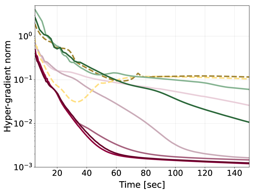
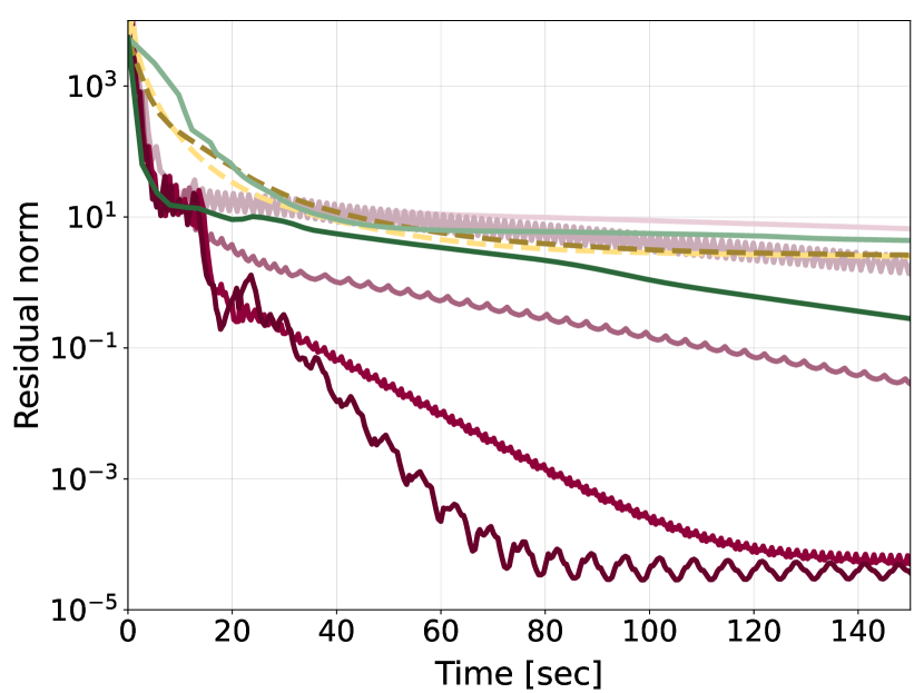
Figure 5: Influence of the subspace dimension $m$ on LancBiO. The post-fix of legend represents the subspace dimension $m$ or the inner iteration $I$. Left: norm of the hyper-gradient; Right: residual norm of the linear system, $\left\|{A_{k}v_{k}-b_{k}}\right\|$.

Denote the residual

$$\bar{r}_{0} :=\bar{b},$$

$$\bar{r}_{j} :=\bar{b}-A_{j}^{*}\Delta v_{j},\quad j=1,2,\ldots,m.$$

The following lemma reveals that the dynamic process yields an improved solution for the subproblem (10).

Lemma 3.12.

Suppose Assumptions 3.1, 3.2, 3.3, 3.6, 3.9, 3.10, and 3.11 hold. Within each epoch, we set the step size $\theta\sim\mathcal{O}({1}/{m^{4}})$ a constant for $y$ and the step size for $x$ as zero in the first $m_{0}\sim\mathcal{O}(1)$ steps, and the others as an appropriate constant $\lambda\sim\mathcal{O}({1}/{m^{4}})$, then we have the following inequality,

$$\frac{\left\|\bar{r}_{j}\right\|}{\left\|\bar{r}_{0}\right\|}\leq 2\sqrt{\tilde{\kappa}\left(j\right)}\left(\frac{\sqrt{\tilde{\kappa}\left(j\right)}-1}{\sqrt{\tilde{\kappa}\left(j\right)}+1}\right)^{j}+\sqrt{j}L_{gyy}\varepsilon_{j}\tilde{\kappa}\left(j\right),$$

where $\tilde{\kappa}\left(j\right):=\frac{L_{gy}+\frac{2\sqrt{3}}{3}\left(j+1\right)^{3}L_{gyy}\varepsilon_{j}}{\mu_{g}-\frac{2\sqrt{3}}{3}\left(j+1\right)^{3}L_{gyy}\varepsilon_{j}}.$

Theorem 3.13.

Suppose Assumptions 3.1, 3.2, 3.3, 3.6, 3.9, 3.10 and 3.11 hold. Within each epoch, we set the step size as $\theta\sim\mathcal{O}({1}/{m^{4}})$ a constant for $y$ and the step size for $x$ as zero in the first $m_{0}$ steps, and the others as a constant $\lambda\sim\mathcal{O}({1}/{m^{4}})$, then the iterates $\{x_{k}\}$ generated by Algorithm 2 satisfy

$$\frac{m}{K\left(m-m_{0}\right)}\sum_{\footnotesize\begin{subarray}{c}k=0,\\ (k\,\emph{{mod}}\,m)>m_{0}\end{subarray}}^{K}{\left\|\nabla\varphi\left(x_{k}\right)\right\|^{2}}\leq\mathcal{O}\left(\frac{m\lambda^{-1}}{K\left(m-m_{0}\right)}\right),$$

where $m_{0}\sim\mathcal{O}(\log m)$ is a constant and $m$ is the subspace dimension.

In other words, we prove that the proposed LancBiO is globally convergent, and the average norm square of the hyper-gradient $\left\|{\nabla\varphi(x_{k})}\right\|^{2}$ achieves $\epsilon$ within $\mathcal{O}(\epsilon^{-1})$ outer iterations.

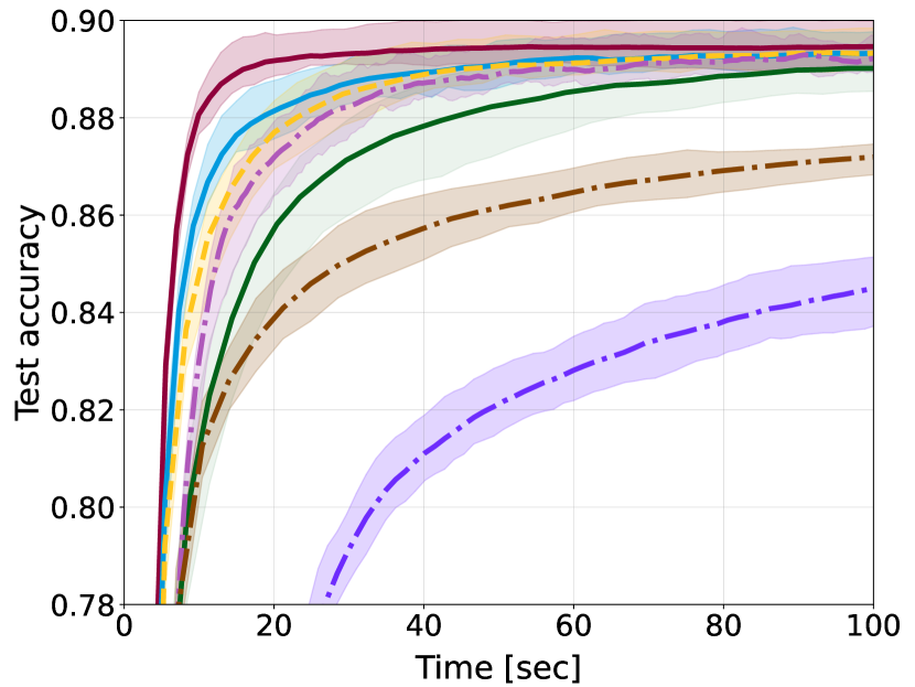
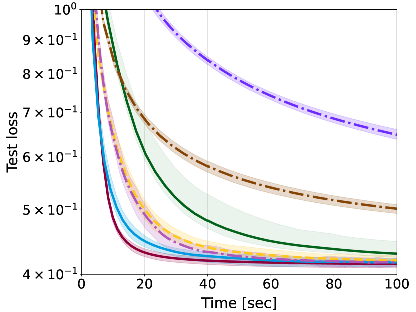
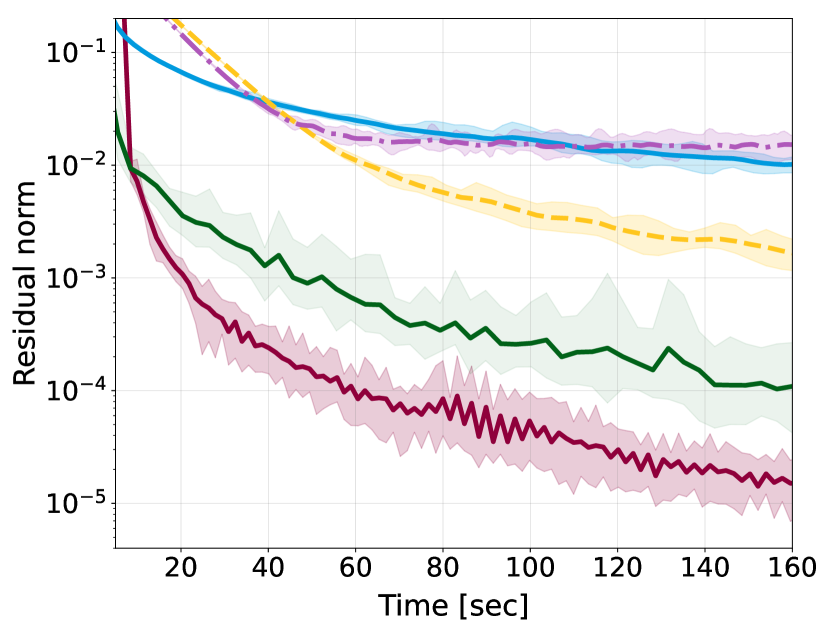
Figure 6: Comparison of the bilevel algorithms on data hyper-cleaning task when $p=0.8$. Left: test accuracy; Center: test loss; Right: residual norm of the linear system, $\left\|{A_{k}v_{k}-b_{k}}\right\|$.

Table 1: Comparison of the bilevel algorithms on data hyper-cleaning task across two corruption rates $p=0.5$ and $p=0.8$. The results are averaged over $10$ runs and $\pm$ is followed by the standard deviation. The results are conducted after $40$ and $60$ seconds running time.

Algorithm	$p=0.5$			$p=0.8$
	Test accuracy (%)	Test loss	Residual	Test accuracy   (%)	Test loss	Residual
LancBiO	${90.35\pm 0.1716}$	${0.36\pm 0.0028}$	${1.20}\mathrm{e}{-4}\pm{2.52}\mathrm{e}{-5}$	${89.45\pm 0.2470}$	${0.42\pm 0.0038}$	${{9.18}\mathrm{e}{-5}\pm{2.77}\mathrm{e}{-5}}$
SubBiO	$90.21\pm 0.2159$	$0.36\pm 0.0035$	${2.22}\mathrm{e}{-2}\pm{2.63}\mathrm{e}{-3}$	$89.22\pm 0.2587$	$0.42\pm 0.0050$	${2.49}\mathrm{e}{-2}\pm{1.93}\mathrm{e}{-3}$
AmIGO-GD	$90.16\pm 0.2114$	$0.37\pm 0.0044$	${3.66}\mathrm{e}{-2}\pm{4.00}\mathrm{e}{-3}$	$89.14\pm 0.2722$	$0.43\pm 0.0044$	${1.07}\mathrm{e}{-2}\pm{8.25}\mathrm{e}{-4}$
AmIGO-CG	$90.06\pm 0.2305$	$0.38\pm 0.0053$	${5.89}\mathrm{e}{-4}\pm{2.52}\mathrm{e}{-4}$	$88.57\pm 0.5839$	$0.46\pm 0.0176$	${6.32}\mathrm{e}{-4}\pm{3.74}\mathrm{e}{-4}$
SOBA	$90.00\pm 0.1811$	$0.37\pm 0.0051$	${2.74}\mathrm{e}{-2}\pm{8.52}\mathrm{e}{-3}$	$88.99\pm 0.2661$	$0.42\pm 0.0054$	${1.73}\mathrm{e}{-2}\pm{1.70}\mathrm{e}{-3}$
TTSA	$89.35\pm 0.2747$	$0.40\pm 0.0103$	-	$82.91\pm 0.4516$	$0.74\pm 0.0072$	-
stocBiO	$89.20\pm 0.1824$	$0.43\pm 0.0033$	-	$86.44\pm 0.2907$	$0.54\pm 0.0064$	-

4 Numerical Experiments

In this section, we conduct experiments in the deterministic setting to empirically validate the performance of the proposed algorithms. We test on a synthetic problem and two deep learning tasks. The selection of parameters and more details of the experiments are deferred to Appendix I. We have made the code publicly available on https://github.com/UCAS-YanYang/LancBiO.

Synthetic problem: We concentrate on a synthetic scenario in bilevel optimization (1) with $d_{x}=d_{y}=d$ and

$$f(x,y):= ~{}c_{1}\cos\left({x^{\top}D_{1}y}\right)+\frac{1}{2}\left\|{D_{2}x-y}\right\|^{2},$$

$$g(x,y):= ~{}c_{2}\sum_{i=1}^{d}{\sin(x_{i}+y_{i})}+\log\left({\sum_{i=1}^{d}{e^{x_{i}y_{i}}}}\right)$$

$$+\frac{1}{2}y^{\top}\left({D_{3}+G}\right)y.$$

It can be seen from Figure 8 that LancBiO achieves the final accuracy the fastest, which benefits from the more accurate $v^{*}$ estimation. Figure 5 illustrates how variations in $m$ and $I$ influence the performance of LancBiO and AmIGO, tested across a range from $10$ to $150$ for $m$, and from $2$ to $10$ for $I$. For clarity, we set the seed of the experiment at $4$, and present typical results to encapsulate the observed trends. It is observed that the increase of $m$ accelerates the decrease in the residual norm, thus achieving better convergence of the hyper-gradient, which aligns with the spirit of the classic Lanczos process. Under the same outer iterations, to attain a comparable convergence property, $I$ for AmIGO-CG should be set to $10$. Furthermore, given that the number of Hessian-vector products averages at $(1+\frac{1}{m})$ per outer iteration for LancBiO, whereas AmIGO requires $I\geq 2$, it follows that LancBiO is more efficient.

Data hyper-cleaning on MNIST: The data hyper-cleaning task (Shaban et al., 2019), conducted on the MNIST dataset (LeCun et al., 1998), aims to train a classifier in a corruption scenario, where the labels of the training data are randomly altered to incorrect classification numbers at a certain probability $p$, referred to as the corruption rate.

The results are presented in Figure 6 and Table 1. Note that LancBiO is crafted for approximating the Hessian inverse vector product $v^{*}$, while the two solid methods, TTSA and stocBiO are not. Consequently, with respect to the residual norm of the linear system, i.e., $\left\|{A_{k}v_{k}-b_{k}}\right\|$, we only compare the results with AmIGO-GD, AmIGO-CG and SOBA. Observe that the proposed subspace-based LancBiO achieves the lowest residual norm and the best test accuracy, and subBiO is comparable to the other algorithms. Specifically, in Figure 6, the efficiency of LancBiO stems from its accurate approximation of the linear system. Additionally, while AmIGO-CG is also adept at approximating $v^{*}$, the green line in Figure 6 indicates that it tends to yield results with higher variance.

Logistic regression on $20$Newsgroup: Consider the hyper-parameters selection task on the $20$Newsgroups dataset (Grazzi et al., 2020), which contains $c=20$ topics with around $18000$ newsgroup posts represented in a feature space of dimension $l=130107$. The goal is to simultaneously train a linear classifier $w$ and determine the optimal regularization parameter $\zeta$. As shown in Figure 11, AmIGO-CG exhibits slightly better performance in reducing the residual norm. Nevertheless, under the same time, LancBiO implements more outer iterations to update $x$, which optimizes the hyper-function more efficiently.

Generally, for standard linear systems, the traditional Lanczos process is recognized for its efficiency and versatility over gradient descent methods. LancBiO, in a sense, reflects this principle within the context of bilevel optimization, underscoring the effectiveness of the dynamic Lanczos-aided approach.

5 Conclusion and Perspective

This paper presents a novel approach to bilevel optimization through the dynamic Lanczos process to approximate Krylov subspaces, to address the computational challenges inherent in calculating the hyper-gradient. The theoretical analysis and empirical validation of LancBiO underscore its reliability and effectiveness. The proposed framework is limited to the deterministic setting. The incorporation of stochastic subspace techniques could unlock better potential in wider applications.

Appendix A Related Work in Bilevel Optimization

A variety of bilevel optimization algorithms are based on reformulation. These algorithms involve transforming the lower-level problem into a set of constraints, such as the optimal conditions of the lower-level problem (Dempe & Dutta, 2012; Li et al., 2023), or the optimal value condition (Outrata, 1990; Ye & Zhu, 1995, 2010; Dempe & Zemkoho, 2013; Lin et al., 2014; Xu & Ye, 2014). Furthermore, incorporating the constraints of the reformulated problem as the penalty function into the upper-level objective inspires a series of algorithms (Liu et al., 2022; Hu et al., 2023; Kwon et al., 2023a, b; Lu & Mei, 2023). Another category of methods in bilevel optimization is the iterative differentiation (ITD) based method (Maclaurin et al., 2015; Franceschi et al., 2017; Shaban et al., 2019; Grazzi et al., 2020; Liu et al., 2020; Ji et al., 2021), which takes advantage of the automatic differentiation technique. Central to this approach is the construction of a computational graph during each outer iteration, achieved by solving the lower-level problem. This setup facilitates the approximation of the hyper-gradient through backpropagation, and it is noted that parts of these methods share a unified structure, characterized by recursive equations (Ji et al., 2021; Li et al., 2022; Zhang et al., 2023). The approximate implicit differentiation (AID) treats the lower-level variable as a function of the upper-level variable. It calculates the hyper-gradient to implement alternating gradient descent between the two levels (Ghadimi & Wang, 2018; Ji et al., 2021; Chen et al., 2022; Dagréou et al., 2022; Li et al., 2022; Hong et al., 2023).

Appendix B Krylov Subspace and Lanczos Process

Krylov subspace (Krylov, 1931) is fundamental in numerical linear algebra (Parlett, 1998; Saad, 2011; Golub & Van Loan, 2013) and nonlinear optimization (Yuan, 2014; Liu et al., 2021), specifically in the context of solving large linear systems and eigenvalue problems. We will briefly introduce the Krylov subspace and the Lanczos process, and recap some important properties; readers are referred to Saad (2011); Golub & Van Loan (2013) for more details.

An $N$-dimensional Krylov subspace generated by a matrix $A$ and a vector $b$ is defined as follows,

$$\mathcal{K}_{N}(A,b):=\operatorname{span}\left\{b,Ab,A^{2}b,\ldots,A^{N-1}b\right\},$$

and the sequence of vectors $\left\{b,Ab,A^{2}b,\ldots,A^{N-1}b\right\}$ forms the basis for it. The Krylov subspace is widely acknowledged for its favorable properties in various aspects, including approximating eigenvalues (Kuczyński & Woźniakowski, 1992), solving the regularized nonconvex quadratic problems (Gould et al., 1999; Zhang et al., 2017; Carmon & Duchi, 2018), and reducing computation cost (Brown & Saad, 1990; Bellavia & Morini, 2001; Liu et al., 2013; Jiang et al., 2024).

The Lanczos process (Lanczos, 1950) is an algorithm that exploits the structure of the Krylov subspace when $A$ is symmetric. Specifically, in the $j$-th step of the Lanczos process, we can efficiently maintain an orthogonal basis $Q_{j}$ of $\mathcal{K}_{j}(A,b)$, so that $T_{j}=Q_{j}^{\top}AQ_{j}$ is tridiagonal, which means a tridiagonal matrix $T_{j}$ approximates $A$ in the Krylov subspace. Consequently, it allows to solve the minimal residual problem or the eigenvalue problem efficiently within the Krylov subspace. There are several equivalent variants of the Lanczos process (Paige, 1971, 1976; Meurant & Strakoš, 2006), and we follow the update rule as shown in Algorithm 3.

Algorithm 3 Lanczos process

0:  dimension $m$, matrix $A\in\mathbb{R}^{n\times n}$, initial vector $b\in\mathbb{R}^{n}$

1:  Initialization: $q_{1}=\frac{b}{\left\|{b}\right\|}$, $q_{0}=\bf{0}$, $\beta_{1}=0$, $Q_{0}=T_{0}=\texttt{Empty Matrix}$

2:  for $j=1,2,\dots,m$ do

3:     $u_{j}=Aq_{j}-\beta_{j}q_{j-1}$

4:     $\alpha_{j}=q_{j}^{\top}u_{j}$

5:     $\omega_{j}=u_{j}-\alpha_{j}q_{j}$

6:     $\beta_{j+1}=\left\|\omega_{j}\right\|$

7:     $q_{j+1}=\omega_{j}/\beta_{j+1}$

8:     $Q_{j}=[Q_{j-1}\ q_{j}]$

9:     $T_{j}={\left(\begin{array}[]{ccc:c}&&&\\ &\phantom{{\small ss}}{\Large T_{j-1}}&&\\ &&&\beta_{j}\vphantom{{\small\frac{2}{\frac{2}{3}}}}\\ \hdashline&&\beta_{j}\phantom{{\small s}}&\alpha_{j}\\ \end{array}\right)}$

10:  end for

10:  $T_{m},Q_{m},\left\|{b}\right\|e_{1}$

We now present several key properties of the Krylov subspace and the Lanczos Process from Saad (2011).

Definition B.1.

The minimal polynomial of a vector $v\in\mathbb{R}^{n}$ with respect to a matrix $A\in\mathbb{R}^{n\times n}$ is defined as the non-zero monic polynomial $p$ of the lowest degree such that $p(A)v=0$, where a monic polynomial is a non-zero univariate polynomial with the coefficient of highest degree equal to $1$.

Remark B.2.

The degree of the minimal polynomial $p$ does not exceed $n$ because the set of $n\!+\!1$ vectors $\{A^{n}v,A^{n-1}v,\ldots,A^{2}v,Av,v\}$ is linearly dependent.

Remark B.3.

Suppose the minimal polynomial of a vector $v$ with respect to a matrix $A$ is

$$p(x)=x^{m}+c_{m-1}x^{m-1}+\cdots+c_{2}x^{2}+c_{1}x+c_{0},$$

and has a degree of $m$. If $c_{0}\neq 0$ and $A$ is invertible, by Definition B.1,

$$A^{m}v+c_{m-1}A^{m-1}v+\cdots+c_{2}A^{2}v+c_{1}Av+c_{0}v=0,$$

multiply both sides of the equation by $A^{-1}$ and rearrange the equation,

$$v=-\frac{1}{c_{0}}\left(A^{m-1}v+c_{m-1}A^{m-2}v+\cdots+c_{2}Av+c_{1}v\right).$$

In other words, $A^{-1}v$ belongs to the Krylov subspace $\mathcal{K}_{m}(A,v)$.

Proposition B.4.

Denote the $n\times j$ matrix with column vectors $q_{1},\ldots,q_{j}$ by $Q_{j}$ and the $j\times m$ tridiagonal matrix by $T_{j}$, all of which are generated by Algorithm 3. Then the following 3-term recurrence holds.

$$AQ_{j} =Q_{j}T_{j}+\beta_{j+1}q_{j+1}e_{j}^{\top},$$

$$Q_{j}^{\top}AQ_{j} =T_{j}.$$

Based on Proposition B.4, the Lanczos process is illustrated in Figure 7

Figure 7: Classic 3-term recurrence

Appendix C Dynamic Lanczos Subroutine

This section lists the DLanczos subroutine (Algorithm 4) invoked in the LancBiO framework (Algorithm 2). One of the main differences between Algorithm 3 and Algorithm 4 is that Algorithm 3 represents the entire $m$-step Lanczos process, while Algorithm 4 serves as a one-step subroutine. Specifically, LancBiO invokes DLanczos once in each outer iteration (line 11 in Algorithm 2), expanding both $T$ and $Q$ by one dimension. Consequently, the inputs of Algorithm 4 are not indexed to avoid confusion, with their corresponding variables $(T_{k-1},Q_{k-1},A_{k},\beta_{k})$ in Algorithm 2 evolving across outer iterations indexed by $k$. Another difference lies in the dynamic property of the DLanczos subroutine, i.e., the matrix $A_{k}$ passed during each invocation in Algorithm 2 varies, while the classic Lanczos process (Algorithm 3) employs a static $A$.

Algorithm 4 Dynamic Lanczos subroutine for LancBiO (DLanczos)

0:  tridiagonal matrix $T$, basis matrix $Q$ with $j$ columns, Hessian matrix $A$, and $\beta$

1:  if  $j=1$ then

2:     $[q_{1}]=Q,\ q_{-1}={\bf{0}}$

3:  else

4:     $[q_{1},q_{2},\ldots,q_{j}]=Q$

5:  end if

6:  $u_{j}=Aq_{j}-\beta q_{j-1}$

7:  $\alpha_{j}=q_{j}^{\top}u_{j}$

8:  $\omega_{j}=u_{j}-\alpha_{j}q_{j}$

9:  $\beta_{j+1}=\left\|{\omega_{j}}\right\|$

10:  $q_{j+1}=\omega_{j}/{\beta_{j+1}}$

11:  $Q_{j+1}=[Q\ q_{j+1}]$

12:  $T_{j+1}={\left(\begin{array}[]{ccc:c}&&&\\ &\phantom{{\small ss}}{\Large T}&&\\ &&&\beta\vphantom{{\small\frac{2}{\frac{2}{3}}}}\\ \hdashline&&\beta\phantom{{\small s}}&\phantom{{\small s}}\alpha_{j}\\ \end{array}\right)}$

12:  $T_{j+1},Q_{j+1},\beta_{j+1}$

Appendix D Extending LancBiO to Non-convex Lower-level Problem

The Lanczos process is known for its efficiency of constructing Krylov subspaces and is capable of solving indefinite linear systems (Greenbaum et al., 1999). In this section, we will briefly demonstrate that the dynamic Lanczos-aided Bilevel Optimization framework, LancBiO, can also handle lower-level problems with the indefinite Hessian.

Suppose $A$ is invertible, and consider solving a standard linear system

$$Ax=b,$$

with initial ponit $x_{0}$, initial residual $r_{0}=b-Ax_{0}$ and initial error $e_{0}=A^{-1}b-x_{0}$. If the matrix $A$ is positive-definite, the classic Lanczos algorithm is equivalent to the Conjugate Gradient (CG) algorithm (Hestenes et al., 1952), both of which minimize the $A$-norm of the error in an affine space (Greenbaum, 1997; Meurant & Strakoš, 2006), i.e., at the $m$-th step,

$$x_{m}=\!\!\!\operatorname*{arg\,min}_{x\in x_{0}+\mathcal{K}_{m}(A,b)}\left\|{A^{-1}b-x}\right\|_{A}.$$

If the matrix $A$ is not positive-definite, MINRES (Paige & Saunders, 1975) is the algorithm recognized to minimize the 2-norm of the residual in an affine space (Greenbaum, 1997; Meurant & Strakoš, 2006), i.e., at the $m$-th step,

$$x_{m}=\!\!\!\operatorname*{arg\,min}_{x\in x_{0}+\mathcal{K}_{m}(A,b)}\left\|{b-Ax}\right\|.$$ (13)

Additionally, based on $Q_{m}$ as the basis of the Krylov subspace $\mathcal{K}_{m}(A,b)$, $T_{m}$ as the projection of $A$ onto $\mathcal{K}_{m}(A,b)$, and the 3-term recurrence

$$AQ_{m}=Q_{m}T_{m}+\beta_{m+1}q_{m+1}e_{m}^{\top},$$

we can rewrite (13) as

$$x_{m}=x_{0}+Q_{m}c_{m},$$

with

$$c_{m}= \operatorname*{arg\,min}_{c}\left\|{r_{0}-AQ_{m}c}\right\|$$

$$= \operatorname*{arg\,min}_{c}\left\|{r_{0}-Q_{m+1}T_{m+1,m}c}\right\|$$

$$= \operatorname*{arg\,min}_{c}\left\|{Q_{m+1}\left(\left\|{r_{0}}\right\|e_{1}-T_{m+1,m}c\right)}\right\|$$

$$= \operatorname*{arg\,min}_{c}\left\|{\left\|{r_{0}}\right\|e_{1}-T_{m+1,m}c}\right\|,$$

where

$$T_{m+1,m}:=\left[\begin{array}[]{c}T_{m}\\ \beta_{m+1}e_{m}^{\top}\\ \end{array}\right].$$

In the spirit of MINRES, to address the bilevel problem where the lower-level problem exhibits an indefinite Hessian, the framework LancBiO (Algorithm 2) requires only a minor modification. Specifically, line 13 in Algorithm 2, , which solves a small-size tridiagonal linear system, will be replaced by solving a low-dimensional least squares problem

$$c_{k}=\operatorname*{arg\,min}_{c}\left\|{\left\|{r_{k}}\right\|e_{1}-T_{k+1,k}c}\right\|^{2},$$

and computing the correction

$$\Delta v_{k}=Q_{k}c_{k},$$

where

$$T_{k+1,k}:=\left[\begin{array}[]{c}T_{k}\\ \beta_{k+1}e_{k}^{\top}\\ \end{array}\right].$$

Appendix E Proof of Smoothness of $y^{*}$ and $\varphi$

To ensure completeness, in this subsection, we provide detailed proofs for the preliminary lemmas that characterize the smoothness of the lower level solution $y^{*}$ and the hyper-objective $\varphi$.

Lemma E.1.

Under the Assumptions 3.2 and 3.3, $y^{*}(x)$ is $\frac{L_{gx}}{\mu_{g}}$-Lipschitz continuous, i.e., for any $x_{1},x_{2}\in\mathbb{R}^{d_{x}}$,

$$\left\|{y^{*}(x_{1})-y^{*}(x_{2})}\right\|\leq\frac{L_{gx}}{\mu_{g}}\left\|{x_{1}-x_{2}}\right\|.$$

Proof.

The assunption that $\nabla_{x}g(x,y)$ is $L_{gx}$-Lipschitz reveals $\left\|{\nabla^{2}_{xy}g(x,y)}\right\|\leq L_{gx}$. Then

$$\left\|\nabla y^{*}\left(x\right)\right\|=\left\|\nabla_{xy}^{2}g\left(x,y\right)\left[\nabla_{yy}^{2}g\left(x,y\right)\right]^{-1}\right\|\leq\left\|\nabla_{xy}^{2}g\left(x,y\right)\right\|\left\|\left[\nabla_{yy}^{2}g\left(x,y\right)\right]^{-1}\right\|\leq\frac{L_{gx}}{\mu_{g}},$$

since $g(x,\cdot)$ is $\mu_{g}$-strongly convex. ∎

Lemma E.2.

Under the Assumptions 3.1, 3.2 and 3.3, the hyper-gradient $\nabla\varphi(x)$ is $L_{\varphi}$-Lipschitz continuous, i.e., for any $x_{1},x_{2}\in\mathbb{R}^{d_{x}}$,

$$\left\|{\nabla\varphi(x_{1})-\nabla\varphi(x_{2})}\right\|\leq L_{\varphi}\left\|{x_{1}-x_{2}}\right\|,$$

where $L_{\varphi}=\left(1+\frac{L_{gy}}{\mu_{g}}\right)\left(L_{fx}+\frac{L_{gx}L_{fy}+L_{gxy}C_{fy}}{\mu_{g}}+\frac{L_{gx}C_{fy}L_{gyy}}{\mu_{g}^{2}}\right)$.

Proof.

By combining

$$\left(A_{1}^{*}\right)^{-1}b_{1}^{*}-\left(A_{2}^{*}\right)^{-1}b_{2}^{*}$$

$$= \left(A_{1}^{*}\right)^{-1}b_{1}^{*}-\left(A_{1}^{*}\right)^{-1}b_{2}^{*}+\left(A_{1}^{*}\right)^{-1}b_{2}^{*}-\left(A_{2}^{*}\right)^{-1}b_{2}^{*}$$

$$= \left(A_{1}^{*}\right)^{-1}\left(b_{1}^{*}-b_{2}^{*}\right)+\left(A_{1}^{*}\right)^{-1}\left(A_{2}^{*}-A_{1}^{*}\right)\left(A_{2}^{*}\right)^{-1}b_{2}^{*}$$

with the properties revealed by Assumptions 3.1 3.2 and 3.3, we can derive

$$\left\|\left(A_{1}^{*}\right)^{-1}b_{1}-\left(A_{2}^{*}\right)^{-1}b_{2}\right\|\leq\frac{L_{fy}}{\mu_{g}}\left(1+\frac{L_{gy}}{\mu_{g}}\right)\left\|x_{1}-x_{2}\right\|+\frac{C_{fy}L_{gyy}}{\mu_{g}^{2}}\left(1+\frac{L_{gy}}{\mu_{g}}\right)\left\|x_{1}-x_{2}\right\|.$$

In a similar way, we can derive

$$\nabla\varphi\left(x_{1}\right)-\nabla\varphi\left(x_{2}\right)= \left(\nabla_{x}f\left(x_{1},y^{*}\left(x_{1}\right)\right)-\nabla_{x}f\left(x_{2},y^{*}\left(x_{2}\right)\right)\right)$$

$$-\nabla^{2}_{xy}g\left(x_{1},y^{*}\left(x_{1}\right)\right)\left(A_{1}^{*}\right)^{-1}b_{1}^{*}+\nabla^{2}_{xy}g\left(x_{1},y^{*}\left(x_{1}\right)\right)\left(A_{2}^{*}\right)^{-1}b_{2}^{*}$$

$$+\nabla^{2}_{xy}g\left(x_{2},y^{*}\left(x_{2}\right)\right)\left(A_{2}^{*}\right)^{-1}b_{2}^{*}-\nabla^{2}_{xy}g\left(x_{1},y^{*}\left(x_{1}\right)\right)\left(A_{2}^{*}\right)^{-1}b_{2}^{*}.$$

It follows that

$$\left\|\nabla\varphi\left(x_{1}\right)-\nabla\varphi\left(x_{2}\right)\right\|\leq ~{}L_{fx}\left(1+\frac{L_{gy}}{\mu_{g}}\right)\left\|x_{1}-x_{2}\right\|$$

$$+L_{gx}\left(1+\frac{L_{gy}}{\mu_{g}}\right)\left(\frac{L_{fy}}{\mu_{g}}+\frac{C_{fy}L_{gyy}}{\mu_{g}^{2}}\right)\left\|x_{1}-x_{2}\right\|$$

$$+L_{gxy}\frac{C_{fy}}{\mu_{g}}\left(1+\frac{L_{gy}}{\mu_{g}}\right)\left\|x_{1}-x_{2}\right\|$$

$$\leq ~{}L_{\varphi}\left\|x_{1}-x_{2}\right\|,$$

where $L_{\varphi}=\left(1+\frac{L_{gy}}{\mu_{g}}\right)\left(L_{fx}+\frac{L_{gx}L_{fy}+L_{gxy}C_{fy}}{\mu_{g}}+\frac{L_{gx}C_{fy}L_{gyy}}{\mu_{g}^{2}}\right)$. ∎

Appendix F Properties of Dynamic Subspace in Section 3.1

In this section, we focus on the properties of the basis matrix $Q$ and the tridiagonal matrix $T$ constructed within each epoch of the dynamic Lanczos process. Denote

$$A_{k}^{*}=\nabla_{yy}^{2}g\left(x_{k},y^{*}_{k}\right)\text{ and }b_{k}^{*}=\nabla_{y}f\left(x_{k},y^{*}_{k}\right).$$

An epoch is constituted of a complete $m$-step dynamic Lanczos process between two restarts, namely, after $h$ epochs, the number of outer iterations is $mh$. Given the outer iterations $k=mh+j$ for $j=1,2,\ldots,m$, we denote

$$\varepsilon_{st}^{h}:=\left(1+\frac{L_{gx}}{\mu_{g}}\right)\left\|x_{mh+s}-x_{mh+t}\right\|+\left\|y_{mh+s}-y_{mh+s}^{*}\right\|$$

for $s,t=1,2,\dots,m$ and

$$\varepsilon_{j}^{h}:=\max_{1\leq s,t\leq j}\varepsilon_{st}^{h},$$

serving as the accumulative difference. For brevity, we omit the superscript where there is no ambiguity, and we are slightly abusing of notation that at the current epoch, $\{A_{mh+j}\}$ and $\{b_{mh+j}\}$ are simplified by $\{A_{j}\}$ and $\{b_{j}\}$ for $j=1,\dots,m$. In addition, the approximations in the residual system (9) are simplified by $\bar{v}$ and $\bar{b}:=b_{1}-A_{1}\bar{v}$.

We rewrite dynamic update rule from Section 2.2

$$u_{j} =A_{j}q_{j}-\beta_{j}q_{j-1},$$ (14)

$$\alpha_{j} =q_{j}^{\top}u_{j},$$ (15)

$$\omega_{j} =u_{j}-\alpha_{j}q_{j},$$ (16)

$$\beta_{j+1} =\left\|\omega_{j}\right\|,$$ (17)

$$q_{j+1} =\omega_{j}/\beta_{j+1},$$ (18)

for $j=1,2,\ldots,m$ with $q_{0}=\mathbf{0}\ ,\beta_{1}=0$ and $Q_{1}=q_{1}=\bar{b}/\left\|{\bar{b}}\right\|$. The following proposition characterizes that the dynamic subspace constructed in Algorithm 2 within an epoch is indeed an approximate Krylov subspace.

Proposition F.1.

At the $j$-th step within an epoch ($j=1,2,\ldots,m-1$), the subspace spanned by the matrix $Q_{j+1}$ in Algorithm 2 satisfies

$$\mathrm{span}(Q_{j+1})\subseteq\mathrm{span}\left\{A_{1}^{a_{1}}A_{2}^{a_{2}}\cdots A_{j}^{a_{j}}\bar{b}\,\left|\!\begin{array}[]{c}a_{s}=0\ \text{\emph{or}}\ 1\\ \forall s=1,2,\ldots,j\\ \end{array}\!\right.\!\right\}.$$ (19)

Specifically, when $A_{1}=A_{2}=\cdots=A_{j}=A$ and $Q_{j+1}$ is of full rank,

$$\mathrm{span}(Q_{j+1})=\mathcal{K}_{j+1}\left({A,\bar{b}}\right)$$

Proof.

Note that $Q_{1}=\mathrm{span}\{q_{1}\}$ with $q_{1}=\frac{\bar{b}}{\left\|{\bar{b}}\right\|}$ satisfies (19). We will give a proof by induction. Suppose for $i=1,2,\ldots,j$,

$$\mathrm{span}(Q_{i+1})\subseteq\mathrm{span}\left\{A_{1}^{a_{1}}A_{2}^{a_{2}}\cdots A_{i}^{a_{i}}\bar{b}\,\left|\!\begin{array}[]{c}a_{s}=0\ \text{or}\ 1\\ \forall s=1,2,\ldots,i\\ \end{array}\!\right.\!\right\}.$$

By the dynamic Lanczos process, it yields

$$q_{j+2}=\frac{1}{\beta_{j+2}}\left(A_{j+1}q_{j+1}-\beta_{j+1}q_{j}-\alpha_{j+1}q_{j+1}\right).$$ (20)

Since

$$q_{j+1}\in\mathrm{span}\left\{A_{1}^{a_{1}}A_{2}^{a_{2}}\cdots A_{j}^{a_{j}}\bar{b}\,\,\left|\begin{array}[]{c}a_{s}=0\ \text{or}\,\,a_{s}=1\\ \forall s=1,2,\ldots,j\\ \end{array}\right.\right\},$$

then we have

$$A_{j+1}q_{j+1}\in\mathrm{span}\left\{A_{1}^{a_{1}}A_{2}^{a_{2}}\cdots A_{j+1}^{a_{j}+1}\bar{b}\,\,\left|\begin{array}[]{c}a_{s}=0\ \text{or}\,\,a_{s}=1\\ \forall s=1,2,\ldots,j+1\\ \end{array}\right.\right\}.$$

It follows from (20) that

$$q_{j+2}\in\mathrm{span}\left\{A_{1}^{a_{1}}A_{2}^{a_{2}}\cdots A_{j+1}^{a_{j}+1}\bar{b}\,\,\left|\begin{array}[]{c}a_{s}=0\ \text{or}\,\,a_{s}=1\\ \forall s=1,2,\ldots,j+1\\ \end{array}\right.\right\}.$$

By induction, we complete the proof. ∎

Although we can estimate the difference between the basis of the above two subspaces, it is noted that the Krylov subspaces can be very sensitive to small perturbation (Meurant & Strakoš, 2006). Therefore, a more detailed observation of the dynamic Lanczos process is necessary, together with the development of relevant lemmas adapted from existing work (Paige, 1976, 1980; Greenbaum, 1997) to support our analysis.

Lemma F.2.

Suppose Assumptions 3.1 to 3.3 hold. The dynamic Lanczos process in Algorithm 2 with normalized $q_{1}$ and $\alpha_{j},\beta_{j},q_{j}$ satisfies

$$A_{j}^{*}Q_{j}=Q_{j}T_{j}+\beta_{j+1}q_{j+1}e_{j}^{\top}+\delta Q_{j}$$ (21)

for $j=1,2,\dots,m$, where $Q_{j}=\left[q_{1},q_{2},\dots,q_{j}\right]$, $\delta Q_{j}=\left[\delta q_{1},\delta q_{2},\dots,\delta q_{j}\right]$,

$$T_{j}=\begin{pmatrix}\alpha_{1}&\beta_{2}&&&&\\ \beta_{2}&\alpha_{2}&\beta_{3}&&&\\ &\beta_{3}&\ddots&\ddots&\\ &&\ddots&\ddots&\beta_{j}&\\ &&&\beta_{j}&\alpha_{j}&\\ \end{pmatrix}.$$

The columns of the perturbation $\delta Q_{j}$ satisfy

$$\left\|{\delta q_{i}}\right\|\leq L_{gyy}\varepsilon_{j},\text{ for }i=1,2,\dots,j.$$

Additionally, if we decompose $Q_{j}$ as

$$Q^{\top}_{j}Q_{j}=R_{j}^{\top}+R_{j},$$ (22)

with $R_{j}$ as a strictly upper triangular matrix, then

$$T_{j}R_{j}-R_{j}T_{j}=\beta_{j+1}Q_{j}^{\top}q_{j+1}e_{j}^{\top}+\delta R_{j},$$ (23)

where $\delta R_{j}$ is strictly upper triangular with elements $\left|{\zeta_{st}}\right|\leq 2L_{gyy}\varepsilon_{j}$, for $1\leq s<t\leq j$.

Proof.

From

$$\alpha_{j}=q_{j}^{\top}u_{j}=q_{j}^{\top}A_{j}q_{j}-\beta_{j}q_{j}^{\top}q_{j-1}$$

and

$$q_{j+1}^{\top}q_{j}=\frac{1}{\beta_{j+1}}\omega_{j}^{\top}q_{j}=\frac{1}{\beta_{j+1}}\left(u_{j}-\alpha_{j}q_{j}\right)^{\top}q_{j}=\frac{1}{\beta_{j+1}}\left(A_{j}q_{j}-\alpha_{j}q_{j}-\beta_{j}q_{j-1}\right)^{\top}q_{j},$$

we can derive

$$q^{\top}_{j+1}q_{j}=0$$ (24)

by induction. Then, we combine equations (14), (15), (16) and (18), and rewrite them in the perturbed form:

$$\beta_{i+1}q_{i+1}=A_{i}q_{i}-\beta_{i}q_{i-1}-\alpha_{i}q_{i}=A_{j}^{*}q_{i}-\beta_{i}q_{i-1}-\alpha_{i}q_{i}+\delta q_{i},\ \ for\ i=1,2,\dots,j,$$ (25)

where $\left\|\delta q_{i}\right\|\leq L_{gyy}\varepsilon_{j}$ due to Assumpstions 3.2 and 3.3. Specifically, (25) can be rewritten in a compact form:

$$A_{j}^{*}Q_{j}=Q_{j}T_{j}+\beta_{j+1}q_{j+1}e_{j}^{\top}+\delta Q_{j}.$$

Then, we will consider the orthogonality of matrix $Q_{j}$, which is reflected by $R_{j}$ in (22). Multiply Equation 21 on the left by $Q^{\top}_{j}$,

$$Q_{j}^{\top}A_{j}^{*}Q_{j}=Q_{j}^{\top}Q_{j}T_{j}+\beta_{j+1}Q_{j}^{\top}q_{j+1}e_{j}^{\top}+Q_{j}^{\top}\delta Q_{j}.$$

Combine its symmetry with the decomposition (22), then

$$T_{j}\left(R_{j}^{\top}+R_{j}\right)-\left(R_{j}^{\top}+R_{j}\right)T_{j}=\beta_{j+1}\left(Q_{j}^{\top}q_{j+1}e_{j}^{\top}-e_{j}q_{j+1}^{\top}Q_{j}\right)+Q_{j}^{\top}\delta Q_{j}-\delta Q_{j}^{\top}Q_{j}.$$ (26)

Denote $M_{j}=T_{j}R_{j}-R_{j}T_{j}$ which is upper triangular. Since the consecutive $q_{i}$ is orthogonal as revealed by (24), we can conclude that the diagnoal elements of $M_{j}$ are $0$. Furthermore, by extracting the upper triangular part of the right hand side of (26), we can get

$$M_{j}=T_{j}R_{j}-R_{j}T_{j}=\beta_{j+1}Q_{j}^{\top}q_{j+1}e_{j}^{\top}+\delta R_{j},$$

where $\delta R_{j}$ is strictly upper triangular with elements $\zeta_{st}$ satisfying: for $t=2,3,\ldots,j$,

$$\left\{\begin{array}[]{cl}\zeta_{t-1,t}&=q_{t-1}^{\top}\delta q_{t}-\delta q_{t-1}^{\top}q_{t}\\ \zeta_{st}&=q_{s}^{\top}\delta q_{t}-\delta q_{s}^{\top}q_{t},\ \ \ \ \quad\ \ s=1,2,\dots,t-2.\\ \end{array}\right.$$

From the bound of $\left\|{\delta q_{j}}\right\|$ it follows that for $1\leq s<t\leq j$, $\left|{\zeta_{st}}\right|\leq 2L_{gyy}\varepsilon_{j}$. ∎

Lemma F.2 illustrates the influence of the dynamics in Algorithm 2 imposed on the standard 3-term Lanczos recurrence, and as (22) reveals, $R$ characterizes the loss of orthogonality of the basis $Q$. However, the following lemmas demonstrate that the range of eigenvalues of the approximate projection matrix $T$ is controllable.

To begin with, we establish the Ritz pairs of $T_{j}$ as $\left(\mu_{i}^{\left(j\right)},y_{i}^{\left(j\right)}\right)$ for $i=1,2,\dots,j$, such that

$$T_{j}Y^{(j)}=Y^{(j)}\operatorname{diag}\left(\mu_{1}^{(j)},\mu_{2}^{(j)},\ldots,\mu_{j}^{(j)}\right).$$

where the normalized $\{y^{(j)}_{i}\}_{i=1}^{j}$ form the orthogonal matrix $Y^{(j)}$ with the elements $\varsigma^{(j)}_{st}$ for $1\leq s,t\leq j$, and we arrange the Ritz values in a specific order,

$$\mu_{1}^{(j)}>\mu_{2}^{(j)}>\cdots>\mu_{j}^{(j)}.$$

We define the $j$-th approximate eigenvector matrix

$$Z^{\left(j\right)}:=\left[z_{1}^{\left(j\right)},z_{2}^{\left(j\right)},\dots,z_{j}^{\left(j\right)}\right]:=Q_{j}Y^{\left(j\right)}.$$

and the corresponding Rayleigh quotients of $A_{j}^{*}$

$$\nu^{(j)}_{i}:=\frac{\left(z_{i}^{\left(j\right)}\right)^{\top}A_{j}^{*}z_{i}^{\left(j\right)}}{\left(z_{i}^{\left(j\right)}\right)^{\top}z_{i}^{\left(j\right)}},\text{ for}\ i=1,2,\dots,j.$$

The subsequent lemma presents a description for the difference of eigenvalues between $T_{j}$ and the tridiagonal matrix in the preceding steps.

Lemma F.3.

Suppose Assumptions 3.1 to 3.3 hold. For any eigenpair $\left(\mu_{i}^{\left(j\right)},y_{i}^{\left(j\right)}\right)$ of $T_{j}$, there exists an integer pair $(s,n)$ where $1\leq s\leq n<j$, such that

$$\left|{\mu_{i}^{\left(j\right)}-\mu_{s}^{\left(n\right)}}\right|\leq\frac{2j^{2}L_{gyy}\varepsilon_{j}}{\sqrt{3}\left|\left(y_{i}^{\left(j\right)}\right)^{\top}R_{j}y_{i}^{\left(j\right)}\right|}.$$ (27)

Proof.

Multiply the eigenvector $y_{r}^{\left(i\right)}$ of $T_{i}$ by $T_{j}$, where $i<j$,

$$T_{j}\left[\begin{array}[]{c}y_{r}^{\left(i\right)}\\ \mathbf{0}\\ \end{array}\right]=\left[\begin{array}[]{c}\mu_{r}^{\left(i\right)}y_{r}^{\left(i\right)}\\ \beta_{r+1}\varsigma_{ir}^{\left(i\right)}e_{1}\\ \end{array}\right].$$ (28)

Then multiply $\left(y_{s}^{\left(j\right)}\right)^{\top}$ on the both sides of (28),

$$\left(\mu_{s}^{\left(j\right)}-\mu_{r}^{\left(i\right)}\right)\left(y_{s}^{\left(j\right)}\right)^{\top}\left[\begin{array}[]{c}y_{r}^{\left(i\right)}\\ \mathbf{0}\\ \end{array}\right]=\beta_{i+1}\varsigma_{ir}^{\left(i\right)}\varsigma_{i+1,s}^{\left(j\right)},$$ (29)

and multiply the eigenvectors $\left(y_{s}^{\left(j\right)}\right)^{\top}$ and $y_{t}^{\left(j\right)}$ on the left and right of (23), respectively,

$$\left(\mu_{s}^{\left(j\right)}-\mu_{t}^{\left(j\right)}\right)\left(y_{s}^{\left(j\right)}\right)^{\top}R_{j}y_{t}^{\left(j\right)}=\varsigma_{jt}^{\left(j\right)}\beta_{j+1}\left(z_{s}^{\left(j\right)}\right)^{\top}q_{j+1}+\epsilon_{st}^{\left(j\right)},$$ (30)

where we difine

$$\epsilon_{st}^{\left(j\right)}:=\left(y_{s}^{\left(j\right)}\right)^{\top}\delta R_{j}y_{t}^{\left(j\right)}.$$ (31)

Note that $\left|\epsilon_{st}^{\left(j\right)}\right|\leq 2jL_{gyy}\varepsilon_{j}$ because of F.2. Specifically, by taking $s=t$ in (30),

$$\left(z_{s}^{\left(j\right)}\right)^{\top}q_{j+1}=-\frac{\epsilon_{ss}^{\left(j\right)}}{\beta_{j+1}\varsigma_{js}^{\left(j\right)}},$$ (32)

and we can rewrite (32) in the matrix form

$$Q_{r}^{\top}q_{r+1}=Y^{\left(r\right)}c_{r},$$ (33)

where for $r=1,\ldots,s$,

$$e_{s}^{\top}c_{r}:=-\frac{\epsilon_{ss}^{\left(r\right)}}{\beta_{r+1}\varsigma_{rs}^{\left(j\right)}}.$$

By observing that $Q_{r}^{\top}q_{r+1}=Y^{\left(r\right)}c_{r}$ is the $(r+1)$-th column of $R_{j}$, we can derive

$$\left(y_{i}^{\left(j\right)}\right)^{\top}R_{j}y_{i}^{\left(j\right)} =-\sum_{r=1}^{j-1}{\varsigma_{r+1,i}^{\left(j\right)}}\sum_{t=1}^{r}{\frac{\epsilon_{tt}^{\left(r\right)}}{\beta_{r+1}\varsigma_{rt}^{\left(r\right)}}\left(y_{i}^{\left(j\right)}\right)^{\top}\left[\begin{array}[]{c}y_{t}^{\left(r\right)}\\ \mathbf{0}\\ \end{array}\right]}$$ (36)

$$=-\sum_{r=1}^{j-1}{\left(\varsigma_{r+1,i}^{\left(j\right)}\right)^{2}}\sum_{t=1}^{r}{\frac{\epsilon_{tt}^{\left(r\right)}}{\mu_{i}^{\left(j\right)}-\mu_{t}^{\left(r\right)}}},$$ (37)

where (36) and (37) follow from (33) and (29) respectively. Consequently, the definition (31) reveals

$$\sum_{s,t=1}^{j}{\left(\epsilon_{st}^{\left(j\right)}\right)^{2}}=\left\|\delta R_{j}\right\|_{F}^{2}\leq 2j^{2}L_{gyy}\varepsilon_{j}.$$ (38)

Based on (37) and the orthogonality of $Y^{(j)}$,

$$\left|\left(y_{i}^{\left(j\right)}\right)^{\top}R_{j}y_{i}^{\left(j\right)}\right| \leq\left|\sum_{r=1}^{j-1}{\varsigma_{r+1,i}^{\left(j\right)}}\sum_{t=1}^{r}{\frac{\epsilon_{tt}^{\left(r\right)}}{\min\limits_{1\leq d\leq l<j}\left|{\mu_{i}^{\left(j\right)}-\mu_{d}^{\left(l\right)}}\right|}}\right|$$

$$\leq\frac{1}{\min\limits_{1\leq d\leq l<j}\left|{\mu_{i}^{\left(j\right)}-\mu_{d}^{\left(l\right)}}\right|}\left|\sum_{r=1}^{j-1}\sum_{t=1}^{r}{\varsigma_{r+1,i}^{\left(j\right)}\epsilon_{tt}^{\left(r\right)}}\right|,$$

and it follows from the Cauchy–Schwarz inequality and (38),

$$\min_{1\leq d\leq l<j}\left|{\mu_{i}^{\left(j\right)}-\mu_{d}^{\left(l\right)}}\right|\leq\frac{\sqrt{j}\sqrt{\sum_{r=1}^{j-1}{\sum_{t=1}^{r}{\left(\epsilon_{tt}^{\left(r\right)}\right)^{2}}}}}{\left|\left(y_{i}^{\left(j\right)}\right)^{\top}R_{j}y_{i}^{\left(j\right)}\right|}\,\,\leq\frac{\sqrt{j}\sqrt{\sum_{r=1}^{j-1}{r^{2}\left(2L_{gyy}\varepsilon_{j}\right)^{2}}}}{\left|\left(y_{i}^{\left(j\right)}\right)^{\top}R_{j}y_{i}^{\left(j\right)}\right|}\leq\frac{2j^{2}L_{gyy}\varepsilon_{j}}{\sqrt{3}\left|\left(y_{i}^{\left(j\right)}\right)^{\top}R_{j}y_{i}^{\left(j\right)}\right|}.$$

∎

Lemma F.4.

Suppose Assumptions 3.1 to 3.3 hold. $Q_{j}$ and $T_{j}$ are the basis matrix and the approximate tridiagonal matrix in the $j$-th step and $R_{j}$ is the strictly upper triangular matrix defined in (22) characterizing the orthogonality of $Q_{j}$. Suppose $\mu_{i}^{\left(j\right)}$ is the $i$-th eigenvalue of $T_{j}$, then for $i=1,\ldots,j$,

$$\mu_{g}-\frac{2\sqrt{3}}{3}\left(j+1\right)^{3}L_{gyy}\varepsilon_{j}\leq\mu^{(j)}_{i}\leq L_{gy}+\frac{2\sqrt{3}}{3}\left(j+1\right)^{3}L_{gyy}\varepsilon_{j}.$$ (39)

Proof.

By conducting the left multiplication with $\left(y_{i}^{\left(j\right)}Q_{j}\right)^{\top}$ and the right multiplication with $y_{i}^{\left(j\right)}$ on both sides of equation (21), we obtain the following.

$$\left(z_{i}^{\left(j\right)}\right)^{\top}A_{j}^{*}z_{i}^{\left(j\right)}-\mu_{i}^{\left(j\right)}\left(z_{i}^{\left(j\right)}\right)^{\top}z_{i}^{\left(j\right)}=-\epsilon_{ii}^{\left(j\right)}+\left(z_{i}^{\left(j\right)}\right)^{\top}\delta Q_{j}y_{i}^{\left(j\right)}.$$

Divide by $\left(z_{i}^{\left(j\right)}\right)^{\top}z_{i}^{\left(j\right)}$,

$$\left|\frac{\left(z_{i}^{\left(j\right)}\right)^{\top}A_{j}^{*}z_{i}^{\left(j\right)}-\mu_{i}^{\left(j\right)}\left(z_{i}^{\left(j\right)}\right)^{\top}z_{i}^{\left(j\right)}}{\left(z_{i}^{\left(j\right)}\right)^{\top}z_{i}^{\left(j\right)}}\right|\leq\frac{\left|\epsilon_{ii}^{\left(j\right)}\right|+\left|\left(z_{i}^{\left(j\right)}\right)^{\top}\delta Q_{j}y_{i}^{\left(j\right)}\right|}{\left|1+2\left(y_{i}^{\left(j\right)}\right)^{\top}R_{j}y_{i}^{\left(j\right)}\right|}\leq\frac{\left|\epsilon_{ii}^{\left(j\right)}\right|+L_{gyy}\varepsilon_{j}\sqrt{j\left(\left|1+2\left(y_{i}^{\left(j\right)}\right)^{\top}R_{j}y_{i}^{\left(j\right)}\right|\right)}}{\left|1+2\left(y_{i}^{\left(j\right)}\right)^{\top}R_{j}y_{i}^{\left(j\right)}\right|},$$ (40)

since

$$\left\|z_{i}^{\left(j\right)}\right\|^{2}=1+2\left(y_{i}^{\left(j\right)}\right)^{\top}R_{j}y_{i}^{\left(j\right)}.$$ (41)

Case I: If

$$\left(y_{i}^{\left(j\right)}\right)^{\top}R_{j}y_{i}^{\left(j\right)}<\frac{3}{8}-\frac{\varepsilon_{j}}{2}$$ (42)

holds, then from (41),

$$\left\|z_{i}^{\left(j\right)}\right\|\geq\frac{1}{2}.$$

Furthermore, (40) reveals that there exists a Rayleigh quotient $\nu^{(j)}$ of $A^{*}_{j}$ that satisfies

$$\left|\nu^{\left(j\right)}-\mu_{i}^{\left(j\right)}\right|\leq 2\left|\epsilon_{ii}^{\left(j\right)}\right|+\sqrt{2j}L_{gyy}\varepsilon_{j}\leq\left(4j+\sqrt{2j}\right)L_{gyy}\varepsilon_{j}.$$

Case II: If the condition (42) does not hold, by applying Lemma F.3, we can find an integer pair $(s_{1},n_{1})$ with $1\leq s_{1}\leq n_{1}<j$ such that

$$\left|\mu_{i}^{\left(j\right)}-\mu_{s_{1}}^{\left(n_{1}\right)}\right|\leq\frac{2j^{2}L_{gyy}\varepsilon_{j}}{\sqrt{3}\left|\left(y_{i}^{\left(j\right)}\right)^{\top}R_{j}y_{i}^{\left(j\right)}\right|}\leq 2\sqrt{3}j^{2}L_{gyy}\varepsilon_{j}.$$

By observing that $\left(\mu_{s_{1}}^{\left(n_{1}\right)},y_{s_{1}}^{\left(n_{1}\right)}\right)$ and $\left(y_{s_{1}}^{\left(n_{1}\right)}\right)^{\top}R_{n_{1}}y_{s_{1}}^{\left(n_{1}\right)}$ can also be categorized into Case I or Case II, repeat this process and construct a sequence $\{(s_{t},n_{t})\}_{t=0}^{l+1}$ with $1\leq n_{l+1}<n_{l}<\cdots<n_{1}<n_{0}=j$ until

$$\left(y_{s_{l+1}}^{\left(n_{l+1}\right)}\right)^{\top}R_{j}y_{s_{l+1}}^{\left(n_{l+1}\right)}<\frac{3}{8}-\frac{\varepsilon_{n_{l+1}}}{2}.$$

Inequality (42) holds when the superscript $j=1$ since $T_{1}=[\alpha_{1}],\ y_{1}^{(1)}=1$ and $z^{(1)}_{1}=q_{1}$. Therefore, we will build up $\{(s_{t},n_{t})\}_{t=0}^{l+1}$ in finite steps, resulting in the following estimation.

$$\left|\bar{\nu}^{\left(j\right)}-\mu_{i}^{\left(j\right)}\right| \leq\left|\bar{\nu}^{\left(j\right)}-\mu_{s_{l+1}}^{\left(n_{l+1}\right)}\right|+\sum_{t=0}^{l}{\left|\mu_{s_{t+1}}^{\left(n_{t+1}\right)}-\mu_{s_{t}}^{\left(n_{l}\right)}\right|}$$

$$\leq\left(4j+\sqrt{2j}\right)L_{gyy}\varepsilon_{j}+\sum_{t=0}^{l}{2\sqrt{3}n_{t}^{2}L_{gyy}\varepsilon_{j}}$$

$$\leq\frac{2\sqrt{3}}{3}\left(j+1\right)^{3}L_{gyy}\varepsilon_{j},$$

for some $\bar{\nu}^{\left(j\right)}$.

Any Rayleigh quotient of $A_{j}^{*}$ is bounded by its eigenvalues (Parlett, 1998), i.e., for any $\nu^{(j)}$,

$$\lambda_{min}^{(j)}\leq\nu^{(j)}\leq\lambda_{max}^{(j)},$$

where $\lambda_{min}^{(j)}$ and $\lambda_{max}^{(j)}$ are the minimum and maximal eigenvalue of $A_{j}^{*}$, respectively. Based on 3.2 and 3.3, we thus complete the proof. ∎

Appendix G Proof of Lemma 3.12

G.1 Proof sketch

The proof of Lemma 3.12 is structured by four principal steps.

Step1: extending $\varepsilon_{j}$ to $\tilde{\varepsilon}_{j}$ within the lemmas detailed in Appendix F.

In Appendix F, we adopt $A^{*}_{j}$ and $b^{*}_{j}$ as reference values with each epoch for the analysis, i.e., for $j=1,2,\ldots,m$,

$$A_{j}^{*}:=\nabla_{yy}^{2}g\left(x_{j},y_{j}^{*}\right),\ b_{j}^{*}:=\nabla_{y}f\left(x_{j},y_{j}^{*}\right),\ \bar{b}:=b_{1}-A_{1}\bar{v},\ \bar{r}_{0}:=\bar{b},\ \bar{r}_{j}:=\bar{b}-A_{j}^{*}\Delta v_{j}.$$

and

$$\varepsilon_{j}:=\max_{1\leq s,t\leq j}\left(1+\frac{L_{gx}}{\mu_{g}}\right)\left\|x_{mh+s}-x_{mh+t}\right\|+\left\|y_{mh+s}-y_{mh+s}^{*}\right\|.$$

Note that we can also view the $A_{1},b_{1}$ as reference values. In this way, we denote the similar quantities

$$A_{j}:=\nabla_{yy}^{2}g\left(x_{j},y_{j}\right),\ b_{j}:=\nabla_{y}f\left(x_{j},y_{j}\right),\ \bar{b}^{\prime}:=b_{1}-A_{1}\bar{v},\ \bar{r}^{\prime}_{0}:=\bar{b}^{\prime},\ \bar{r}^{\prime}_{j}:=\bar{b}^{\prime}-A_{1}\Delta v_{j}.$$ (43)

and

$$\tilde{\varepsilon}_{j}:=\max_{1\leq s,t\leq j}\left\|x_{mh+s}-x_{mh+t}\right\|+\left\|y_{mh+s}-y_{mh+t}\right\|.$$ (44)

Consequently, we extend the lemmas in Appendix F. The results listed in Section G.2 are the recipe of Step2.

Step2: upper-bounding the residual $\left\|{\bar{r}_{j}^{\prime}}\right\|$.

In Section G.3, we then demonstrate that if the value of $\tilde{\varepsilon}_{j}$ is not too large, $\left\|{\bar{r}_{j}^{\prime}}\right\|$ can be bounded, which is an important lemma for Step3.

Step3: controlling $\tilde{\varepsilon}_{j}$ and ${\varepsilon}_{j}$ by induction.

Since the expression of $\tilde{\varepsilon}_{j}$ does not involve $y^{*}$, its magnitude can be controlled by adjusting the step size, implied by (44). With the help of the stability of $\tilde{\varepsilon}_{j}$, we can prove

$$\mu_{g}-\frac{2\sqrt{3}}{3}\left(j+1\right)^{3}L_{gyy}{\varepsilon}_{j}>0.$$ (45)

Step4: proof of Lemma 3.12

Based on the conclusion (45) revealing the benign property of the dynamic process, we achieve the proof of Lemma 3.12.

G.2 Extended lemmas from Appendix F

In this part, we view the $A_{1},b_{1}$ as reference values. In this way, we can institute $A_{j}^{*}$ with $A_{1}$ and $\varepsilon_{j}$ with $\tilde{\varepsilon}_{j}$ in the lemmas from Appendix F, resulting in the extended version of lemmas.

Lemma G.1.

(Extended version of Lemma F.2) Suppose Assumptions 3.1 to 3.3 hold. The dynamic Lanczos process in Algorithm 2 with normalized $q_{1}$ and $\alpha_{j},\beta_{j},q_{j}$ satisfies

$$A_{1}Q_{j}=Q_{j}T_{j}+\beta_{j+1}q_{j+1}e_{j}^{\top}+\delta Q^{\prime}_{j}$$ (46)

for $j=1,2,\dots,m$, where $Q_{j}=\left[q_{1},q_{2},\dots,q_{j}\right]$, $\delta Q^{\prime}_{j}=\left[\delta q^{\prime}_{1},\delta q^{\prime}_{2},\dots,\delta q^{\prime}_{j}\right]$,

$$T_{j}=\begin{pmatrix}\alpha_{1}&\beta_{2}&&&&\\ \beta_{2}&\alpha_{2}&\beta_{3}&&&\\ &\beta_{3}&\ddots&\ddots&\\ &&\ddots&\ddots&\beta_{j}&\\ &&&\beta_{j}&\alpha_{j}&\\ \end{pmatrix}.$$

The columns of the perturbation $\delta Q^{\prime}_{j}$ satisfy

$$\left\|{\delta q^{\prime}_{i}}\right\|\leq L_{gyy}\tilde{\varepsilon}_{j},\text{ for }i=1,2,\dots,j.$$ (47)

Lemma G.2.

(Extended version of Lemma F.4) Suppose Assumptions 3.1 to 3.3 hold. $Q_{j}$ and $T_{j}$ are the basis matrix and the approximate tridiagonal matrix in the $j$-th step. Take $\mu_{i}^{\left(j\right)}$ as the $i$-th eigenvalue of $T_{j}$, then for $i=1,\ldots,j$,

$$\mu_{g}-\frac{2\sqrt{3}}{3}\left(j+1\right)^{3}L_{gyy}\tilde{\varepsilon}_{j}\leq\mu^{(j)}_{i}\leq L_{gy}+\frac{2\sqrt{3}}{3}\left(j+1\right)^{3}L_{gyy}\tilde{\varepsilon}_{j}.$$ (48)

G.3 Proof of Step2

The following lemma demonstrates that if the value of $\tilde{\varepsilon}_{j}$ is not too large, $\left\|{\bar{r}_{j}^{\prime}}\right\|$ can be bounded.

Lemma G.3.

Suppose Assumpsions 3.1 to 3.3 and

$$\mu_{g}-\frac{2\sqrt{3}}{3}\left(j+1\right)^{3}L_{gyy}\tilde{\varepsilon}_{j}>0$$

are satisfied within an epoch. Then, it holds that

$$\frac{\left\|\bar{r}^{\prime}_{j}\right\|}{\left\|\bar{r}^{\prime}_{0}\right\|}\leq 2\sqrt{\tilde{\kappa}^{\prime}\left(j\right)}\left(\frac{\sqrt{\tilde{\kappa}^{\prime}\left(j\right)}-1}{\sqrt{\tilde{\kappa}^{\prime}\left(j\right)}+1}\right)^{j}+\sqrt{j}L_{gyy}\varepsilon_{j}\tilde{\kappa}^{\prime}\left(j\right),$$

where $\tilde{\kappa}^{\prime}\left(j\right):=\frac{L_{gy}+\frac{2\sqrt{3}}{3}\left(j+1\right)^{3}L_{gyy}\tilde{\varepsilon}_{j}}{\mu_{g}-\frac{2\sqrt{3}}{3}\left(j+1\right)^{3}L_{gyy}\tilde{\varepsilon}_{j}}.$

Proof.

Denote the solution in the dynamic subspace in the $j$-th step by

$$\Delta\xi_{j}=\left(T_{j}\right)^{-1}\bar{b}=\left\|{\bar{r}^{\prime}_{0}}\right\|\left(T_{j}\right)^{-1}e_{1},$$ (49)

where $T_{j}$ is nonsingular because of Lemma G.2. By (43), (46), and (49),

$$\bar{r}^{\prime}_{j}=\bar{b}-A_{1}Q_{j}\Delta\xi_{j}=-\beta_{j+1}q_{j+1}e_{j}^{\top}\Delta\xi_{j}-\delta Q^{\prime}_{j}\Delta\xi_{j}.$$

It follows that

$$\frac{\left\|\bar{r}^{\prime}_{j}\right\|}{\left\|\bar{r}^{\prime}_{0}\right\|}\leq\left\|\delta Q^{\prime}_{j}\right\|\left\|\left(T_{j}\right)^{-1}\right\|+\left|\beta_{j+1}e_{j}^{\top}\left(T_{j}\right)^{-1}e_{1}\right|.$$ (50)

The first term on the right side of (50) can be bounded by (47) and (48):

$$\left\|\delta Q^{\prime}_{j}\right\|\left\|\left(T_{j}\right)^{-1}\right\|\leq\sqrt{j}L_{gyy}\tilde{\varepsilon}_{j}\frac{L_{gy}}{\mu_{g}-\frac{2\sqrt{3}}{3}\left(j+1\right)^{3}L_{gyy}\tilde{\varepsilon}_{j}}\leq\sqrt{j}L_{gyy}\tilde{\varepsilon}_{j}\tilde{\kappa}^{\prime}\left(j\right).$$ (51)

Recall that

$$T_{j+1,j}:=\left[\begin{array}[]{c}T_{j}\\ \beta_{j+1}e_{j}^{\top}\\ \end{array}\right],$$ (52)

and that for any symmetric tridiagonal matrix $T$, where the upper left $(j+1)\times j$ block is $T_{j+1,j}$, the application of the classic Lanczos algorithm to $T$, starting with the initial vector $e_{1}$ will result in the matrix $T_{j+1,j}$ at the $j$-th step. To construct a suitable $(j+1)\times(j+1)$ symmetric tridiagonal matrix T, we consider a virtual step with ${\lambda^{\diamond}}={\theta^{\diamond}}=0$, which leads to $(x^{\diamond}_{j+1},y^{\diamond}_{j+1})=\left({x_{j},y_{j}}\right)$, $\tilde{\varepsilon}^{\diamond}_{j+1}=\tilde{\varepsilon}_{j}$, and

$$T={\left(\begin{array}[]{ccc:c}&&&\\ &\vphantom{{\small\frac{2^{2^{2^{2}}}}{\frac{2}{3}}}}{\Large T_{j+1,j}}\phantom{s}&&\\ &&&\beta_{j+1}\vphantom{{\small\frac{2}{\frac{2}{3}}}}\\ &&&\tilde{\alpha}^{\diamond}_{j+1}\\ \end{array}\right)}$$

By Lemma G.2, given any eigenvalue $\mu$ of $T$

$$\mu_{g}-\frac{2\sqrt{3}}{3}\left(j+1\right)^{3}L_{gyy}\tilde{\varepsilon}_{j}\leq\mu\leq L_{gy}+\frac{2\sqrt{3}}{3}\left(j+1\right)^{3}L_{gyy}\tilde{\varepsilon}_{j}.$$

In this way, $\left|\beta_{j+1}e_{j}^{\top}\left(T_{j}\right)^{-1}e_{1}\right|$ can be seen as the residual in the $j$-th step of the classic Lanczos process with the positive-definite matrix $T$ and the iniitial vector $e_{1}$. Since the eigenvalues of $T$ satisfy (52), it follows from the standard convergence property of the Lanczos process (Greenbaum, 1997) that

$$\left|\beta_{j+1}e_{j}^{\top}\left(T_{j}\right)^{-1}e_{1}\right|\leq 2\sqrt{\tilde{\kappa}^{\prime}\left(j\right)}\left(\frac{\sqrt{\tilde{\kappa}^{\prime}\left(j\right)}-1}{\sqrt{\tilde{\kappa}^{\prime}\left(j\right)}+1}\right)^{j},$$

which completes the proof. ∎

G.4 Proof details of $\mu_{g}-\frac{2\sqrt{3}}{3}\left(j+1\right)^{3}L_{gyy}{\varepsilon}_{j}>0$

In this part, we will give the detailed proof of $\mu_{g}-\frac{2\sqrt{3}}{3}\left(j+1\right)^{3}L_{gyy}{\varepsilon}_{j}>0$. At the same time, we demonstrate that, with appropriate step sizes, the auxiliary variable $v_{k}$ is bounded, thereby ensuring that the hyper-gradient estimator (5) remains bounded, which ensures the stable behavior of the dynamic Lanczos process,

Lemma G.4.

Suppose Assumptions 3.1, 3.2, 3.3, 3.6, 3.9, 3.10 and 3.11 hold. If within each epoch, we set the step size $\theta\sim\mathcal{O}(\frac{1}{m^{4}})$ a constant for $y$ and the step size for $x$ as zero in the first $m_{0}\sim\mathcal{O}(1)$ steps, and the others as an appropriate constant $\lambda\sim\mathcal{O}(\frac{1}{m^{4}})$, then for any epoch,

$$\mu_{g}-\frac{2\sqrt{3}}{3}\left(j+1\right)^{3}L_{gyy}\varepsilon_{j}>0,\ \text{ for }j=1,2,\ldots,m+1,$$

and there exists a constant $C_{v}>0$ so that $\left\|{v_{k}}\right\|\leq C_{v}$ for ${v_{k}}$ generated by Algorithm 2.

Proof.

Consider the iterates within one epoch and the constants

$$0<\tilde{\varepsilon}<\mu_{g}\text{ and }\tilde{\kappa}:=\frac{L_{gy}+\tilde{\varepsilon}}{\mu_{g}-\tilde{\varepsilon}}.$$

It follows from Lemma G.3 that if $\tilde{\varepsilon}_{j}\leq\frac{\sqrt{3}\tilde{\varepsilon}}{2(m+1)^{3}L_{gyy}}$, then

$$\frac{\left\|b_{1}-A_{1}v_{j}\right\|}{\left\|b_{1}-A_{1}\bar{v}\right\|}\leq 2\sqrt{\tilde{\kappa}}\left(\frac{\sqrt{\tilde{\kappa}}-1}{\sqrt{\tilde{\kappa}}+1}\right)^{j}+\frac{\sqrt{3}\tilde{\varepsilon}}{2(m+1)^{2}}\tilde{\kappa}\leq 3\sqrt{\tilde{\kappa}}.$$ (53)

Then, we will prove by induction. At the beginning of the algorithm, the condition (53) reveals

$$\varepsilon_{1}=\left\|y_{1}-y_{1}^{*}\right\|\leq\frac{\sqrt{3}\mu_{g}}{8\left(m+1\right)^{3}L_{gyy}}.$$

Combining it with $\left\|b_{1}-A_{1}\bar{v}_{0}\right\|\leq C_{r}$ constructs the start of induction within an epoch and induction between epochs. Within an epoch, suppose the following statements hold for $i=1,2,\ldots,j$,

$$\left\|b_{1}-A_{1}v_{i}\right\| \leq 3\sqrt{\tilde{\kappa}}C_{r},$$

$$\left\|v_{i}\right\| \leq\frac{1}{\mu_{g}}\left(3\sqrt{\tilde{\kappa}}C_{r}+C_{fx}\right),$$

$$\left\|\widetilde{\nabla}\varphi_{i}\right\| \leq C_{fx}+\frac{1}{\mu_{g}^{2}}\left(3\sqrt{\tilde{\kappa}}C_{r}+C_{fx}\right),$$

$$\tilde{\varepsilon}_{i} \leq\frac{\sqrt{3}\tilde{\varepsilon}}{2(m+1)^{3}L_{gyy}},$$

$$\varepsilon_{i} \leq\frac{\sqrt{3}\mu_{g}}{4\left(m+1\right)^{3}L_{gyy}}.$$

Then by setting the stepsize

$$\lambda\leq\frac{\sqrt{3}\tilde{\varepsilon}}{4(m+1)^{4}L_{gyy}}\left(C_{fx}+\frac{1}{\mu_{g}^{2}}\left(3\sqrt{\tilde{\kappa}}C_{r}+C_{fx}\right)\right)^{-1},$$

$$\theta\leq\frac{\sqrt{3}\tilde{\varepsilon}}{4(m+1)^{4}L_{gyy}}C_{gy}^{-1},$$

we can get

$$\tilde{\varepsilon}_{j+1}\leq\lambda\sum_{i=1}^{i=j}{\left\|\widetilde{\nabla}\varphi_{i}\right\|}+\theta\sum_{i=1}^{i=j}{\left\|\nabla_{y}g\left(x_{i+1},y_{i}\right)\right\|}\leq\frac{\sqrt{3}\tilde{\varepsilon}}{2(m+1)^{3}L_{gyy}}.$$ (54)

It follows from (53) that

$$\left\|b_{1}-A_{1}v_{j+1}\right\| \leq 3\sqrt{\tilde{\kappa}}C_{r},$$ (55)

$$\left\|v_{j+1}\right\| =\left\|A_{1}^{-1}\left(b_{1}-A_{1}v_{j+1}-b_{1}\right)\right\|\leq\frac{1}{\mu_{g}}\left(3\sqrt{\tilde{\kappa}}C_{r}+C_{fx}\right),$$ (56)

$$\left\|\widetilde{\nabla}\varphi_{j+1}\right\| \leq C_{fx}+\frac{1}{\mu_{g}^{2}}\left(3\sqrt{\tilde{\kappa}}C_{r}+C_{fx}\right).$$ (57)

Additionally, the descent property of $\left\|{y_{s}-y^{*}_{s}}\right\|$ and the Lipschitz continuity of $y^{*}$ reveal that

$$\left\|y_{s}-y_{s}^{*}\right\|\leq \left(1-\theta\mu_{g}\right)^{\frac{1}{2}}\left\|{y_{s-1}-y^{*}_{s}}\right\|$$ (58)

$$\leq \left(1-\theta\mu_{g}\right)^{\frac{1}{2}}\left\|y_{s-1}-y_{s-1}^{*}\right\|+\left(1-\theta\mu_{g}\right)^{\frac{1}{2}}\left(\frac{L_{gx}}{\mu_{g}}\right)\left\|x_{s}-x_{s-1}\right\|$$

$$\leq \left(1-\theta\mu_{g}\right)^{\frac{s-1}{2}}\left\|y_{1}-y_{1}^{*}\right\|+\left(1-\theta\mu_{g}\right)^{\frac{1}{2}}\left(\frac{L_{gx}}{\mu_{g}}\right)\lambda\sum_{t=1}^{t=s-1}{\left\|\widetilde{\nabla}\varphi_{t}\right\|}$$

$$\leq \left\|y_{1}-y_{1}^{*}\right\|+\left(1-\theta\mu_{g}\right)^{\frac{1}{2}}\left(\frac{L_{gx}}{\mu_{g}}\right)\lambda\sum_{t=1}^{t=s-1}{\left\|\widetilde{\nabla}\varphi_{t}\right\|}.$$ (59)

Set

$$\lambda\leq\frac{\sqrt{3}\mu_{g}}{8(m+1)^{4}L_{gyy}}\left(C_{fx}+\frac{1}{\mu_{g}^{2}}\left(3\sqrt{\tilde{\kappa}}C_{r}+C_{fx}\right)\right)^{-1}\left(1+\frac{L_{gx}}{\mu_{g}}+\left(1-\theta\mu_{g}\right)^{\frac{1}{2}}\left(\frac{L_{gx}}{\mu_{g}}\right)\right)^{-1},$$

it yields from (11), (56), (59) that

$$\varepsilon_{j+1}\leq \left(1+\frac{L_{gx}}{\mu_{g}}\right)\max_{1\leq s,t\leq j+1}\left\|x_{s}-x_{t}\right\|+\max_{1\leq s\leq j+1}\left\|y_{s}-y_{s}^{*}\right\|$$

$$\leq \left\|y_{1}-y_{1}^{*}\right\|+\left(1+\frac{L_{gx}}{\mu_{g}}+\left(1-\theta\mu_{g}\right)^{\frac{1}{2}}\left(\frac{L_{gx}}{\mu_{g}}\right)\right)\lambda\sum_{i=1}^{i=j}{\left\|\widetilde{\nabla}\varphi_{i}\right\|}$$

$$\leq \left\|y_{1}-y_{1}^{*}\right\|+\left(1+\frac{L_{gx}}{\mu_{g}}+\left(1-\theta\mu_{g}\right)^{\frac{1}{2}}\left(\frac{L_{gx}}{\mu_{g}}\right)\right)\lambda\sum_{i=1}^{i=j}{\left\|\widetilde{\nabla}\varphi_{i}\right\|}$$

$$\leq \ \frac{\sqrt{3}\mu_{g}}{4\left(m+1\right)^{3}L_{gyy}}.$$ (60)

As for the next epoch, denoting $C_{v}=\frac{1}{\mu_{g}}\left(3\sqrt{\tilde{\kappa}}C_{r}+C_{fx}\right)$ we have

$$\left\|b_{m+1}-A_{m+1}v_{m}\right\| \leq\left(L_{fx}+L_{gyy}C_{{v}}\right)\tilde{\varepsilon}_{m+1}+\left\|b_{1}-A_{1}v_{m}\right\|$$

$$\leq\left(L_{fx}+L_{gyy}C_{{v}}\right)\tilde{\varepsilon}_{m+1}+\left(2\sqrt{\tilde{\kappa}}\left(\frac{\sqrt{\tilde{\kappa}}-1}{\sqrt{\tilde{\kappa}}+1}\right)^{m}+\sqrt{m}L_{gyy}\tilde{\varepsilon}_{m+1}\tilde{\kappa}\right)C_{r}$$

$$\leq C_{r}\left(\left(\frac{L_{fx}+L_{gyy}C_{{v}}}{C_{r}}\right)\tilde{\varepsilon}_{m+1}+2\sqrt{\tilde{\kappa}}\left(\frac{\sqrt{\tilde{\kappa}}-1}{\sqrt{\tilde{\kappa}}+1}\right)^{m}+\sqrt{m}L_{gyy}\tilde{\varepsilon}_{m+1}\tilde{\kappa}\right)$$

$$\leq C_{r},$$ (61)

by setting $m,\tilde{\varepsilon}$ such that

$$\left(\frac{L_{fx}+L_{gyy}C_{{v}}}{C_{r}}\right)\tilde{\varepsilon}_{m+1}+2\sqrt{\tilde{\kappa}}\left(\frac{\sqrt{\tilde{\kappa}}-1}{\sqrt{\tilde{\kappa}}+1}\right)^{m}+\sqrt{m}L_{gyy}\tilde{\varepsilon}_{m+1}\tilde{\kappa}\leq 1.$$

Moreover, since the step size for $x$ is set as zero at the first $m_{0}$ steps in the next epoch, we obtain for $i=1,2,\ldots,m_{0}$,

$$\varepsilon_{m+i}=\left\|y_{m+i}-y_{m+i}^{*}\right\|\leq\left(1-\theta\mu_{g}\right)^{\frac{i}{2}}\left\|y_{m}-y_{m}^{*}\right\|\leq\varepsilon_{m}\leq\frac{\sqrt{3}\mu_{g}}{4\left(m+1\right)^{3}L_{gyy}}.$$ (62)

Specifically,

$$\left\|y_{m+m_{0}}-y_{m+m_{0}}^{*}\right\|\leq\left(1-\theta\mu_{g}\right)^{\frac{m_{0}}{2}}\left\|y_{m}-y_{m}^{*}\right\|\leq\frac{\sqrt{3}\mu_{g}}{8\left(m+1\right)^{3}L_{gyy}}$$ (63)

if we choose $m_{0}$ so that $\left(1-\theta\mu_{g}\right)^{\frac{m_{0}}{2}}\leq\frac{1}{2}$. Therefore, by induction within an epoch (54), (55), (56), (57), (60) and induction between epochs (61), (62), (63), we conclude the lemma. ∎

G.5 Proof of Lemma 3.12

Lemma G.5.

Suppose Assumptions 3.1, 3.2, 3.3, 3.6, 3.9, 3.10 and 3.11 hold. If within each epoch, we set the step size $\theta\sim\mathcal{O}(\frac{1}{m^{4}})$ a constant for $y$ and the step size for $x$ as zero in the first $m_{0}\sim\mathcal{O}(1)$ steps, and the others as an appropriate constant $\lambda\sim\mathcal{O}(\frac{1}{m^{4}})$, then we have the following.

$$\frac{\left\|\bar{r}_{j}\right\|}{\left\|\bar{r}_{0}\right\|}\leq 2\sqrt{\tilde{\kappa}\left(j\right)}\left(\frac{\sqrt{\tilde{\kappa}\left(j\right)}-1}{\sqrt{\tilde{\kappa}\left(j\right)}+1}\right)^{j}+\sqrt{j}L_{gyy}\varepsilon_{j}\tilde{\kappa}\left(j\right),$$

where $\tilde{\kappa}\left(j\right):=\frac{L_{gy}+\frac{2\sqrt{3}}{3}\left(j+1\right)^{3}L_{gyy}\varepsilon_{j}}{\mu_{g}-\frac{2\sqrt{3}}{3}\left(j+1\right)^{3}L_{gyy}\varepsilon_{j}}.$

Proof.

Lemma G.4 guarantees the condition

$$\mu_{g}-\frac{2\sqrt{3}}{3}\left(j+1\right)^{3}L_{gyy}{\varepsilon}_{j}>0$$

is satisfied. The remaining proof can be directly adapted from Lemma G.3. ∎

Appendix H Proof of The Main Theorems

In this section, we provide proof of the main theorem presented in Section 3.2. Let $A_{k}=\nabla_{yy}g(x_{k},y_{k})$ and $b_{k}=\nabla_{y}f(x_{k},y_{k})$, and let the reference values be $A_{k}^{*}=\nabla_{yy}^{2}g\left(x_{k},y^{*}_{k}\right)$, $b^{*}_{k}=\nabla_{y}f\left(x_{k},y^{*}_{k}\right)$ and $v_{k}^{*}=(A_{k}^{*})^{-1}b_{k}^{*}$.

The following lemma displays the descent properties of the iterates $\{y_{k}\}$.

Lemma H.1.

Suppose Assumptions 3.2 and 3.3 hold, we have

$$\left\|y_{k+1}-y_{k+1}^{*}\right\|^{2}\leq\left(1+\sigma\right)\left(1-\theta\mu_{g}\right)\left\|y_{k}-y_{k}^{*}\right\|^{2}+\left(1+\frac{1}{\sigma}\right)\left(1-\theta\mu_{g}\right)\left(\frac{L_{gx}}{\mu_{g}}\right)^{2}\left\|x_{k+1}-x_{k}\right\|^{2},$$

for any $\sigma>0$.

Proof.

Algorithm 2 executes a single-step gradient descent on the strongly convex function $g(x_{k+1},\cdot)$ during the outer iteration. Leveraging the established convergence properties of strongly convex functions (Nesterov et al., 2018), we are thus able to derive the following.

$$\left\|y_{k+1}-y_{k+1}^{*}\right\|^{2}\leq\left(1-\theta\mu_{g}\right)\left\|y_{k}-y_{k+1}^{*}\right\|^{2}.$$

By Young’s inequality that $\left|{a+b}\right|^{2}\leq(1+\sigma)\left|{a}\right|^{2}+\left(1+\frac{1}{\sigma}\right)\left\|b\right\|^{2}$ with any $\sigma>0$,

$$\left\|y_{k+1}-y_{k+1}^{*}\right\|^{2}\leq\left(1+\sigma\right)\left(1-\theta\mu_{g}\right)\left\|y_{k}-y_{k}^{*}\right\|^{2}+\left(1+\frac{1}{\sigma}\right)\left(1-\theta\mu_{g}\right)\left(\frac{L_{gx}}{\mu_{g}}\right)^{2}\left\|x_{k+1}-x_{k}\right\|^{2}.$$

∎

In the context of bilevel optimization, we define the initial residual in the $(h+1)$-th epoch as

$$r_{h+1}:=b_{mh+1}-A_{mh+1}\bar{v}_{h},$$

and the residual in $k$-th step

$$r_{k}:=\left(b_{mh+1}-A_{mh+1}\bar{v}_{h}\right)-A_{k}^{*}\Delta v_{k}.$$

Based on the boundness of $v_{k}$ in Lemma G.4 we can estimate

$$\mu_{g}\left\|v_{k}-v_{k}^{*}\right\|\leq \left\|\left(b_{k}^{*}-A_{k}^{*}\bar{v}_{h}\right)-A_{k}^{*}\Delta v_{k}\right\|$$

$$= \left\|\left(b_{k}^{*}-A_{k}^{*}\bar{v}_{h}\right)-A_{k}^{*}\Delta v_{k}-r_{k}+r_{k}\right\|$$

$$\leq \left\|b_{k}^{*}-b_{mh+1}\right\|+\left\|A_{k}^{*}-A_{mh+1}\right\|\left\|\bar{v}_{h}\right\|+\left\|r_{k}\right\|$$

$$\leq ~{}L_{fy}\left\|\left(x_{k},y_{k}^{*}\right)-\left(x_{mh+1},y_{mh+1}\right)\right\|$$

$$+L_{gyy}\left\|\left(x_{k},y_{k}^{*}\right)-\left(x_{mh+1},y_{mh+1}\right)\right\|\left\|\bar{v}_{h}\right\|+\left\|r_{k}\right\|$$

$$= \left(L_{fy}+L_{gyy}\left\|v_{mh}\right\|\right)\varepsilon_{j}^{h}+\left\|r_{k}\right\|$$

$$\leq \left(L_{fy}+L_{gyy}C_{v}\right)\varepsilon_{j}^{h}+\left\|r_{k}\right\|,$$ (64)

which comes from $\left\|{(A_{j}^{*})^{-1}}\right\|\leq\frac{1}{\mu_{g}}$, $v_{k}=\bar{v}_{h}+\Delta v_{k}$, and $\left\|{v_{k}}\right\|\leq C_{v}$.

Lemma H.2.

Suppose Assumptions 3.1, 3.2, 3.3, 3.6, 3.10 and 3.11 hold. Within each epoch, we set the step size $\theta\sim\mathcal{O}(\frac{1}{m^{4}})$ a constant for $y$ and the step size for $x$ as zero in the first $m_{0}$ steps, and the others as an appropriate constant $\lambda\sim\mathcal{O}(\frac{1}{m^{4}})$, then the iterates

$$\{x_{k}\}\ \text{ for }\ k=mh+j,\ h=0,1,2,\ldots,\ \text{ and }\ j=m_{0}+1,m_{0}+2,\ldots,m,$$

generated by Algorithm 2 satisfy

$$\left\|\widetilde{\nabla}\varphi\left(x_{k}\right)-\nabla\varphi\left(x_{k}\right)\right\|^{2}\leq ~{}3L_{gx}^{2}\iota^{2\left(j-m_{0}\right)+h\left(m-m_{0}\right)}\delta_{0}+18\left(1-\gamma\right)^{-1}\lambda^{2}L_{gx}^{2}m^{2}\omega_{\varphi}\sum_{t=0}^{j-1}{\left\|\nabla\varphi\left(x_{mh+t}\right)\right\|^{2}}$$

$$+18\left(1-\gamma\right)^{-1}\lambda^{2}L_{gx}^{2}m^{2}\omega_{\varphi}\sum_{e=0}^{h-1}{\iota^{2\left(h-e\right)\left(m-m_{0}\right)}\sum_{t=0}^{m-1}{\left\|\nabla\varphi\left(x_{me+t}\right)\right\|^{2}}},$$

where $0<\gamma<1$, $m_{0}\sim\mathcal{O}(\log m)$ are constants, $m$ is the subspace dimension, and $\delta_{0}$ is a constant defined in the proof.

Proof.

By (H), conclusion from Lemma G.3 and the Young’s inequality,

$$\left\|v_{k}-v_{k}^{*}\right\|^{2} \leq 2\left(\frac{L_{fy}+L_{gyy}C_{v}}{\mu_{g}}\right)^{2}\left(\varepsilon_{j}^{h}\right)^{2}+2\frac{1}{\mu_{g}^{2}}\left\|r_{k}\right\|^{2}$$

$$\leq 2\left(\frac{L_{fy}+L_{gyy}C_{v}}{\mu_{g}}\right)^{2}\left(\varepsilon_{j}^{h}\right)^{2}+2\frac{1}{\mu_{g}^{2}}\left(2\sqrt{\tilde{\kappa}\left(j\right)}\left(\frac{\sqrt{\tilde{\kappa}\left(j\right)}-1}{\sqrt{\tilde{\kappa}\left(j\right)}+1}\right)^{j}+\sqrt{j}L_{gyy}\varepsilon_{j}^{h}\tilde{\kappa}\left(j\right)\right)^{2}\left\|r_{k0}\right\|^{2}$$

$$\leq 2\left(\frac{L_{fy}+L_{gyy}C_{v}}{\mu_{g}}\right)^{2}\left(\varepsilon_{j}^{h}\right)^{2}+4\frac{1}{\mu_{g}^{2}}\left(4\tilde{\kappa}\left(j\right)\left(\frac{\sqrt{\tilde{\kappa}\left(j\right)}-1}{\sqrt{\tilde{\kappa}\left(j\right)}+1}\right)^{2j}+\left(\sqrt{j}\tilde{\kappa}\left(j\right)L_{gyy}\right)^{2}\left(\varepsilon_{j}^{h}\right)^{2}\right)\left\|r_{k0}\right\|^{2}.$$

An estimate can be made for $\left\|{r_{h+1}}\right\|$,

$$\left\|{r_{h+1}}\right\|= \left\|b_{mh+1}-A_{mh+1}\bar{v}_{h}\right\|$$

$$= \left\|b_{mh+1}-b_{mh}^{*}+A_{mh}^{*}v_{mh}^{*}-A_{mh+1}v_{mh}\right\|$$

$$\leq ~{}L_{fy}\left\|\left(x_{mh+1},y_{mh+1}\right)-\left(x_{mh},y_{mh}^{*}\right)\right\|$$

$$+\frac{C_{fy}}{\mu_{g}}L_{gyy}\left\|\left(x_{mh+1},y_{mh+1}\right)-\left(x_{mh},y_{mh}^{*}\right)\right\|+L_{gy}\left\|v_{mh}^{*}-v_{mh}\right\|$$

$$= ~{}L_{gy}\left\|v_{mh}-v_{mh}^{*}\right\|+\frac{\mu_{g}L_{fy}+C_{fy}L_{gyy}}{\mu_{g}}\left(1+\frac{L_{gx}}{\mu_{g}}\right)\left\|x_{mh+1}-x_{mh}\right\|,$$

thus

$$\left\|v_{k}-v_{k}^{*}\right\|^{2}\leq ~{}\omega_{\varepsilon}\left(\varepsilon_{j}^{h}\right)^{2}+\frac{L_{gy}^{2}}{\mu_{g}^{2}}\tilde{\kappa}\left(j\right)\left(\frac{\sqrt{\tilde{\kappa}\left(j\right)}-1}{\sqrt{\tilde{\kappa}\left(j\right)}+1}\right)^{2j}\left\|v_{mh}-v_{mh}^{*}\right\|^{2}$$

$$+\frac{\tilde{\kappa}\left(j\right)}{\mu_{g}^{2}}\left(\frac{\mu_{g}L_{fy}+C_{fy}L_{gyy}}{\mu_{g}}\left(1+\frac{L_{gx}}{\mu_{g}}\right)\right)^{2}\left(\frac{\sqrt{\tilde{\kappa}\left(j\right)}-1}{\sqrt{\tilde{\kappa}\left(j\right)}+1}\right)^{2j}\left\|x_{mh+1}-x_{mh}\right\|^{2},$$ (65)

where

$$\omega_{\varepsilon}=2\left(\frac{L_{fy}+L_{gyy}C_{v}}{\mu_{g}}\right)^{2}+\frac{4}{\mu_{g}^{2}}\left(\sqrt{m}\tilde{\kappa}\left(m\right)L_{gyy}\right)^{2}\left(L_{gy}^{2}C_{v}^{2}+\left(\frac{\mu_{g}L_{fy}+C_{fy}L_{gyy}}{\mu_{g}}\left(1+\frac{L_{gx}}{\mu_{g}}\right)\right)^{2}C_{s}^{2}\right)\sim\mathcal{O}\left(m\right).$$

Now, we define

$$\delta_{k}=\left(\frac{L_{fx}^{2}\mu_{g}^{2}+L_{gxy}^{2}C_{fg}^{2}}{L_{gx}^{2}\mu_{g}^{2}}\right)\left\|y_{k}-y_{k}^{*}\right\|^{2}+\left\|v_{k}-v_{k}^{*}\right\|^{2},$$

and add $\left(\frac{L_{fx}^{2}\mu_{g}^{2}+L_{gxy}^{2}C_{fg}^{2}}{L_{gx}^{2}\mu_{g}^{2}}\right)\left\|y_{k}-y_{k}^{*}\right\|^{2}$ on both sides of (H). Combine it with Lemma H.1,

$$\delta_{k}\leq ~{}\omega_{\varepsilon}\left(\varepsilon_{j}^{h}\right)^{2}+\frac{L_{gy}^{2}}{\mu_{g}^{2}}\tilde{\kappa}\left(j\right)\left(\frac{\sqrt{\tilde{\kappa}\left(j\right)}-1}{\sqrt{\tilde{\kappa}\left(j\right)}+1}\right)^{2j}\left\|v_{mh}-v_{mh}^{*}\right\|^{2}$$

$$+\frac{\tilde{\kappa}\left(j\right)}{\mu_{g}^{2}}\left(\frac{\mu_{g}L_{fy}+C_{fy}L_{gyy}}{\mu_{g}}\left(1+\frac{L_{gx}}{\mu_{g}}\right)\right)^{2}\left(\frac{\sqrt{\tilde{\kappa}\left(j\right)}-1}{\sqrt{\tilde{\kappa}\left(j\right)}+1}\right)^{2j}\left\|x_{mh+1}-x_{mh}\right\|^{2}$$

$$+\left(1+\sigma\right)^{j}\left(1-\theta\mu_{g}\right)^{j}\frac{L_{fx}^{2}\mu_{g}^{2}+L_{gxy}^{2}C_{fg}^{2}}{L_{gx}^{2}\mu_{g}^{2}}\left\|y_{mh}-y_{mh}^{*}\right\|^{2}$$

$$+\left(1+\frac{1}{\sigma}\right)\left(1-\theta\mu_{g}\right)\frac{L_{fx}^{2}\mu_{g}^{2}+L_{gxy}^{2}C_{fg}^{2}}{L_{gx}^{2}\mu_{g}^{2}}\left(\frac{L_{gx}}{\mu_{g}}\right)^{2}\sum_{r=0}^{j}{\left(1+\sigma\right)^{r}\left(1-\theta\mu_{g}\right)^{r}\left\|x_{k-r}-x_{k-r-1}\right\|^{2}}.$$ (66)

We set $\sigma,\theta$ to satisfy $\left(1+\sigma\right)\left(1-\theta\mu_{g}\right)<1$, and since Lemma G.4 reveals that under the appropriate step-size setting $\lambda\sim\mathcal{O}(\frac{1}{m^{4}})$ and $\theta\sim\mathcal{O}(\frac{1}{m^{4}})$, $\tilde{\kappa}(j)\leq\tilde{\kappa}$ for some $\tilde{\kappa}>0$, we define

$$\iota:=\max\left\{\frac{\sqrt{\tilde{\kappa}}-1}{\sqrt{\tilde{\kappa}}+1},\sqrt{\left(1+\sigma\right)\left(1-\theta\mu_{g}\right)}\right\}<1$$ (67)

Choose a positive integer $m_{0}$ such that, for $0<\gamma<1$,

$$\iota^{-2m_{0}}\geq(1-\gamma)^{-1}\max\left\{\left(\frac{L_{fx}^{2}\mu_{g}^{2}+L_{gxy}^{2}C_{fg}^{2}}{L_{gx}^{2}\mu_{g}^{2}}\right)^{-1}\left(\frac{L_{fx}^{2}\mu_{g}^{2}+L_{gxy}^{2}C_{fg}^{2}}{L_{gx}^{2}\mu_{g}^{2}}+m\right),\frac{L_{gy}^{2}}{\mu_{g}^{2}}\tilde{\kappa}\left(\frac{\mu_{g}L_{fy}+C_{fy}L_{gyy}}{\mu_{g}}\left(1+\frac{L_{gx}}{\mu_{g}}\right)\right)^{2}\right\},$$

which means $m_{0}\sim\mathcal{O}\left(\log m\right)$.

Since we set the step size for $x$ as zero in the first $m_{0}$ steps, 3.10 reveals that

$$\left(\varepsilon_{j}^{h}\right)^{2}\leq\lambda^{2}m\left(1+\frac{L_{gx}}{\mu_{g}}\right)^{2}\sum_{t=m_{0}}^{j-1}{\left\|\widetilde{\nabla}\varphi\left(x_{mh+t}\right)\right\|}^{2}+m\left\|y_{mh+j}-y_{mh+j}^{*}\right\|^{2},$$

then

$$\delta_{k}\leq ~{}\lambda^{2}m\omega_{\varepsilon}\left(1+\frac{L_{gx}}{\mu_{g}}\right)^{2}\sum_{t=m_{0}}^{j-1}{\left\|\widetilde{\nabla}\varphi\left(x_{mh+t}\right)\right\|}^{2}+\frac{L_{gy}^{2}}{\mu_{g}^{2}}\tilde{\kappa}\left(j\right)\left(\frac{\sqrt{\tilde{\kappa}\left(j\right)}-1}{\sqrt{\tilde{\kappa}\left(j\right)}+1}\right)^{2j}\left\|v_{mh}-v_{mh}^{*}\right\|^{2}$$

$$+\frac{\tilde{\kappa}\left(j\right)}{\mu_{g}^{2}}\left(\frac{\mu_{g}L_{fy}+C_{fy}L_{gyy}}{\mu_{g}}\left(1+\frac{L_{gx}}{\mu_{g}}\right)\right)^{2}\left(\frac{\sqrt{\tilde{\kappa}\left(j\right)}-1}{\sqrt{\tilde{\kappa}\left(j\right)}+1}\right)^{2j}\left\|x_{mh+1}-x_{mh}\right\|^{2}$$

$$+\left(1+\sigma\right)^{j}\left(1-\theta\mu_{g}\right)^{j}\left(\frac{L_{fx}^{2}\mu_{g}^{2}+L_{gxy}^{2}C_{fg}^{2}}{L_{gx}^{2}\mu_{g}^{2}}+m\right)\left\|y_{mh}-y_{mh}^{*}\right\|^{2}$$

$$+\left(1+\frac{1}{\sigma}\right)\left(1-\theta\mu_{g}\right)\left(\frac{L_{fx}^{2}\mu_{g}^{2}+L_{gxy}^{2}C_{fg}^{2}}{L_{gx}^{2}\mu_{g}^{2}}+m\right)\left(\frac{L_{gx}}{\mu_{g}}\right)^{2}\sum_{r=0}^{j}{\left(1+\sigma\right)^{r}\left(1-\theta\mu_{g}\right)^{r}\left\|x_{k-r}-x_{k-r-1}\right\|^{2}}.$$ (68)

Then we can rearrange (H),

$$\delta_{k}\leq(1-\gamma)\iota^{2\left(j-m_{0}\right)}\left(\delta_{mh}\right)+3m^{2}\lambda^{2}\omega_{\varphi}\left(\sum_{t=m_{0}}^{j-1}{\left\|\widetilde{\nabla}\varphi\left(x_{mh+t}\right)\right\|}^{2}+\left\|{\widetilde{\nabla}\varphi(x_{mh})}\right\|^{2}\right),$$ (69)

where we denote

$$\omega_{\varphi}=\max \left\{\frac{\omega_{\varepsilon}}{m}\left(1+\frac{L_{gx}}{\mu_{g}}\right)^{2},\frac{\tilde{\kappa}\iota}{m^{2}\mu_{g}^{2}}\left(\frac{\mu_{g}L_{fy}+C_{fy}L_{gyy}}{\mu_{g}}\left(1+\frac{L_{gx}}{\mu_{g}}\right)\right)^{2},\right.$$

$$\left.\frac{1}{m^{2}}\left(1+\frac{1}{\sigma}\right)\left(1-\theta\mu_{g}\right)\left(\frac{L_{fx}^{2}\mu_{g}^{2}+L_{gxy}^{2}C_{fg}^{2}}{L_{gx}^{2}\mu_{g}^{2}}+m\right)\left(\frac{L_{gx}}{\mu_{g}}\right)^{2}\right\}\sim\mathcal{O}\left(1\right).$$

Since

$$\left\|\widetilde{\nabla}\varphi\left(x_{k}\right)-\nabla\varphi\left(x_{k}\right)\right\|^{2}\leq ~{}3\left\|\nabla_{x}f\left(x_{k},y_{k}\right)-\nabla_{x}f\left(x_{k},y_{k}^{*}\right)\right\|^{2}+3\left\|\nabla_{xy}^{2}g\left(x_{k},y_{k}\right)\right\|^{2}\left\|v_{k}-v_{k}^{*}\right\|^{2}$$

$$+3\left\|\nabla_{xy}^{2}g\left(x_{k},y_{k}\right)-\nabla_{xy}^{2}g\left(x_{k},y_{k}^{*}\right)\right\|^{2}\left\|v_{k}^{*}\right\|^{2}$$

$$\leq ~{}3L_{fx}^{2}\left\|y_{k}-y_{k}^{*}\right\|^{2}+3L_{gx}^{2}\left\|v_{k}-v_{k}^{*}\right\|^{2}+3L_{gxy}^{2}\left(\frac{C_{fy}}{\mu_{g}}\right)^{2}\left\|y_{k}-y_{k}^{*}\right\|^{2}$$

$$= ~{}3L_{gx}^{2}\delta_{k},$$ (70)

it follows that

$$\delta_{k}\leq \left(1-\gamma\right)\iota^{2\left(j-m_{0}\right)}\left(\delta_{mh}\right)+3m^{2}\lambda^{2}\omega_{\varphi}\left(\sum_{t=m_{0}}^{j-1}{\left\|\widetilde{\nabla}\varphi\left(x_{mh+t}\right)\right\|}^{2}+\left\|{\widetilde{\nabla}\varphi(x_{mh})}\right\|^{2}\right)$$

$$\leq \left(1-\gamma\right)\iota^{2\left(j-m_{0}\right)}\left(\delta_{mh}\right)+6\lambda^{2}m^{2}\omega_{\varphi}\left(\sum_{t=m_{0}}^{j-1}{\left\|\widetilde{\nabla}\varphi\left(x_{mh+t}\right)-\nabla\varphi(x_{mh+t})\right\|}^{2}+\left\|{\widetilde{\nabla}\varphi(x_{mh})-\nabla\varphi(x_{mh})}\right\|^{2}\right)$$

$$+6\lambda^{2}m^{2}\omega_{\varphi}\left(\sum_{t=m_{0}}^{j-1}{\left\|{\nabla}\varphi\left(x_{mh+t}\right)\right\|}^{2}+\left\|{{\nabla}\varphi(x_{mh})}\right\|^{2}\right)$$

$$\leq \left(1-\gamma\right)\iota^{2\left(j-m_{0}\right)}\left(\delta_{mh}\right)+18\lambda^{2}L_{gx}^{2}m^{2}\omega_{\varphi}\left(\sum_{t=m_{0}}^{j-1}{\delta_{mh+t}}+\delta_{mh}\right)$$

$$+6\left(1-\gamma\right)\left(1-\gamma\right)^{-1}\lambda^{2}m^{2}\omega_{\varphi}\left(\sum_{t=m_{0}}^{j-1}{\left\|{\nabla}\varphi\left(x_{mh+t}\right)\right\|}^{2}+\left\|{{\nabla}\varphi(x_{mh})}\right\|^{2}\right).$$ (71)

Based on (H), the following inequality can be checked by induction.

$$\delta_{k}\leq\iota^{2\left(j-m_{0}\right)}\left(\delta_{mh}\right)+6\left(1-\gamma\right)^{-1}\lambda^{2}m^{2}\omega_{\varphi}\left(\sum_{t=m_{0}}^{j-1}{\left\|\nabla\varphi\left(x_{mh+t}\right)\right\|^{2}}+\left\|{\nabla\varphi\left(x_{mh}\right)}\right\|^{2}\right),$$

if $\lambda\leq\mathcal{O}\left(m^{-1}\iota^{m}\right)$, specifically,

$$\lambda\leq\min\left\{\left(\frac{\gamma}{18\omega_{\varphi}}\right)^{1/2}\frac{1}{L_{gx}}m^{-3/2},\ \left(\frac{\gamma}{18\omega_{\varphi}}\right)^{1/2}\frac{1}{L_{gx}}m^{-1}\iota^{m-m_{0}}\right\}.$$

Note that we can adjust the step size $\theta$ in (67) such that $\iota$ is closed to $1$, thus for simplicity, we still take $\lambda\sim\mathcal{O}(\frac{1}{m^{4}})$ We can bound $\delta_{k}$ recursively by

$$\delta_{k}\leq ~{}\iota^{2\left(j-m_{0}\right)}\left(\delta_{mh}\right)+6\left(1-\gamma\right)^{-1}\lambda^{2}m^{2}\omega_{\varphi}\sum_{t=0}^{j-1}{\left\|\nabla\varphi\left(x_{mh+t}\right)\right\|^{2}}$$

$$\leq ~{}\iota^{2\left(j-m_{0}\right)+h\left(m-m_{0}\right)}\delta_{0}+6\left(1-\gamma\right)^{-1}\lambda^{2}m^{2}\omega_{\varphi}\sum_{t=0}^{j-1}{\left\|\nabla\varphi\left(x_{mh+t}\right)\right\|^{2}}$$

$$+6\left(1-\gamma\right)^{-1}\lambda^{2}m^{2}\omega_{\varphi}\sum_{e=0}^{h-1}{\iota^{2\left(h-e\right)\left(m-m_{0}\right)}\sum_{t=0}^{m-1}{\left\|\nabla\varphi\left(x_{me+t}\right)\right\|^{2}}},$$

where we are slightly abusing of notation that $\delta_{0}=\left(\frac{L_{fx}^{2}\mu_{g}^{2}+L_{gxy}^{2}C_{fg}^{2}}{L_{gx}^{2}\mu_{g}^{2}}\right)\left\|y_{0}-y_{0}^{*}\right\|^{2}+\left\|v_{0}-v_{0}^{*}\right\|^{2}$ for analysis convenience, while we start from $(x_{1},y_{1},v_{1})$ in Algorithm 2 for the statement convenience in this paper. Substituting (H) into (H) completes the proof.

$$\left\|\widetilde{\nabla}\varphi\left(x_{k}\right)-\nabla\varphi\left(x_{k}\right)\right\|^{2}\leq ~{}3L_{gx}^{2}\delta_{k}$$

$$\leq ~{}3L_{gx}^{2}\iota^{2\left(j-m_{0}\right)+h\left(m-m_{0}\right)}\delta_{0}+18\left(1-\gamma\right)^{-1}\lambda^{2}L_{gx}^{2}m^{2}\omega_{\varphi}\sum_{t=0}^{j-1}{\left\|\nabla\varphi\left(x_{mh+t}\right)\right\|^{2}}$$

$$+18\left(1-\gamma\right)^{-1}\lambda^{2}L_{gx}^{2}m^{2}\omega_{\varphi}\sum_{e=0}^{h-1}{\iota^{2\left(h-e\right)\left(m-k\right)}\sum_{t=0}^{m-1}{\left\|\nabla\varphi\left(x_{me+t}\right)\right\|^{2}}}.$$

∎

Theorem H.3.

Suppose Assumptions 3.1, 3.2, 3.3, 3.6, 3.9 3.10, and 3.11 hold. Within each epoch, we set the step size $\theta\sim\mathcal{O}(\frac{1}{m^{4}})$ a constant for $y$ and the step size for $x$ as zero in the first $m_{0}$ steps, and the others as an appropriate constant $\lambda\sim\mathcal{O}(\frac{1}{m^{4}})$, then the iterates $\{x_{k}\}$ generated by Algorithm 2 satisfy

$$\frac{m}{K\left(m-m_{0}\right)}\sum_{\footnotesize\begin{subarray}{c}k=0,\\ (k\,\emph{{mod}}\,m)>m_{0}\end{subarray}}^{K}{\left\|\nabla\varphi\left(x_{k}\right)\right\|^{2}}\leq\mathcal{O}\left(\frac{m\lambda^{-1}}{K\left(m-m_{0}\right)}\right),$$

where $m_{0}\sim\mathcal{O}(\log m)$ is a constant and $m$ is the subspace dimension.

Proof.

According to Lemma E.2, a gradient descent step results in the decrease in the hyper-gradient $\varphi$:

$$\varphi\left(x_{k+1}\right)\leq ~{}\varphi\left(x_{k}\right)+\left<\nabla\varphi\left(x_{k}\right),x_{k+1}-x_{k}\right>+\frac{L_{\varphi}}{2}\left\|x_{k+1}-x_{k}\right\|^{2}$$

$$\leq ~{}\varphi\left(x_{k}\right)-\left(\frac{\lambda}{2}-\lambda^{2}L_{\varphi}\right)\left\|\nabla\varphi\left(x_{k}\right)\right\|^{2}+\left(\frac{\lambda}{2}+\lambda^{2}L_{\varphi}\right)\left\|\nabla\varphi\left(x_{k}\right)-\widetilde{\nabla}\varphi\left(x_{k}\right)\right\|^{2}$$

$$\leq ~{}\varphi\left(x_{k}\right)-\left(\frac{\lambda}{2}-\lambda^{2}L_{\varphi}\right)\left\|\nabla\varphi\left(x_{k}\right)\right\|^{2}+3\left(\frac{\lambda}{2}+\lambda^{2}L_{\varphi}\right)L_{gx}^{2}\iota^{2\left(j-m_{0}\right)+2h\left(m-m_{0}\right)}\delta_{0}$$

$$+18\left(\frac{\lambda}{2}+\lambda^{2}L_{\varphi}\right)\left(1-\gamma\right)^{-1}\lambda^{2}L_{gx}^{2}m^{2}\omega_{\varphi}\left(\sum_{t=0}^{j-1}{\left\|\nabla\varphi\left(x_{mh+t}\right)\right\|^{2}}+\sum_{e=0}^{h-1}{\iota^{2\left(h-e\right)\left(m-m_{0}\right)}\sum_{t=0}^{m-1}{\left\|\nabla\varphi\left(x_{me+t}\right)\right\|^{2}}}\right).$$

Then, telescoping index from $k=0$ to $k=K=mH$,

$$\left(\frac{\lambda}{2}-\lambda^{2}L_{\varphi}\right)\sum_{\footnotesize\begin{subarray}{c}k=0,\\ (k\,{\texttt{mod}}\,m)>m_{0}\end{subarray}}^{K}{\left\|\nabla\varphi\left(x_{k}\right)\right\|^{2}}$$

$$\leq ~{}\varphi\left(x_{0}\right)-\varphi\left(x^{*}\right)+3\left(\frac{\lambda}{2}+\lambda^{2}L_{\varphi}\right)L_{gx}^{2}\delta_{0}\sum_{h=0}^{H-1}{\iota^{2h\left(m-m_{0}\right)}\sum_{j=m_{0}+1}^{m}{\iota^{2\left(j-m_{0}\right)}}}$$

$$+18\lambda^{2}\left(\frac{\lambda}{2}+\lambda^{2}L_{\varphi}\right)\left(1-\gamma\right)^{-1}L_{gx}^{2}m^{2}\omega_{\varphi}\left(m-m_{0}\right)\sum_{\footnotesize\begin{subarray}{c}k=0,\\ (k\,{\texttt{mod}}\,m)>m_{0}\end{subarray}}^{K}{\left\|\nabla\varphi\left(x_{k}\right)\right\|^{2}\sum_{h=0}^{H-1}{\iota^{2h\left(m-m_{0}\right)}}}$$

$$\leq ~{}\varphi\left(x_{0}\right)-\varphi\left(x^{*}\right)+3\left(\frac{\lambda}{2}+\lambda^{2}L_{\varphi}\right)L_{gx}^{2}\delta_{0}\frac{1-\iota^{2H\left(m-m_{0}\right)}}{1-\iota^{2}}$$

$$+18\lambda^{2}\left(\frac{\lambda}{2}+\lambda^{2}L_{\varphi}\right)\left(1-\gamma\right)^{-1}L_{gx}^{2}m^{2}\omega_{\varphi}\left(m-m_{0}\right)\frac{1-\iota^{2H\left(m-m_{0}\right)}}{1-\iota^{2}}\sum_{\footnotesize\begin{subarray}{c}k=0,\\ (k\,{\texttt{mod}}\,m)>m_{0}\end{subarray}}^{K}{\left\|\nabla\varphi\left(x_{k}\right)\right\|^{2}},$$

where $x^{*}\in\operatorname*{arg\,min}_{x\in\mathbb{R}^{d_{x}}}\varphi(x)$. By selecting a suitable value for $\lambda$ such that

$$\lambda L_{\varphi}+18\lambda\left(\frac{\lambda}{2}+\lambda^{2}L_{\varphi}\right)\left(1-\gamma\right)^{-1}L_{gx}^{2}m^{2}\omega_{\varphi}\left(m-m_{0}\right)\frac{1-\iota^{2H\left(m-m_{0}\right)}}{1-\iota^{2}}\leq\frac{1}{4},$$

we can derive

$$\sum_{\footnotesize\begin{subarray}{c}k=0,\\ (k\,{\texttt{mod}}\,m)>m_{0}\end{subarray}}^{K}{\left\|\nabla\varphi\left(x_{k}\right)\right\|^{2}}\leq\frac{4\left(\varphi\left(x_{0}\right)-\varphi\left(x^{*}\right)\right)}{\lambda}+\left(6+12\lambda L_{\varphi}\right)L_{gx}^{2}\delta_{0}\frac{1-\iota^{2H\left(m-m_{0}\right)}}{1-\iota^{2}},$$

which completes the proof by dividing both sides by $\frac{m-m_{0}}{m}T$. ∎

Appendix I Details on Experiments

I.1 General settings

We conduct experiments to empirically validate the performance of the proposed algorithms. We test on a synthetic problem, a hyper-parameters selection task, and a data hyper-cleaning task. We compare the proposed SubBiO and LancBiO with the existing algorithms in bilevel optimization: stocBiO (Ji et al., 2021), AmIGO-GD and AmIGO-CG (Arbel & Mairal, 2022), SOBA (Dagréou et al., 2022) and TTSA (Hong et al., 2023). The experiments are produced on a server that consists of two Intel® Xeon® Gold 6330 CPUs (total 2$\times$28 cores), 512GB RAM, and one NVIDIA A800 (80GB memory) GPU. The synthetic problem and the deep learning experiments are carried out on the CPUs and the GPU, respectively. For wider accessibility and application, we have made the code publicly available on https://github.com/UCAS-YanYang/LancBiO.

For the proposed LancBiO, we initiate the subspace dimension at $1$, and gradually increase it to $m=10$ for the deep learning experiments and to $m=80$ for the synthetic problem. For all the compared algorithms, we employ a grid search strategy to optimize the parameters. The optimal parameters yield the lowest loss. The experiment results are averaged over $10$ runs

In this paper, we consider the algorithms SubBiO and LancBiO in the deterministic scenario, so we initially compare them against the baseline algorithms with a full batch (i.e., deterministic gradient). In this setting, LancBiO yields favorable numerical results. Moreover, in the data hyper-cleaning task, to facilitate a more effective comparison with algorithms designed for stochastic applications, we implement all compared methods with a small batch size, finding that the proposed methods show competitive performance.

I.2 Synthetic problem

We concentrate on a synthetic scenario in bilevel optimization:

$$\begin{array}[]{cl}\min\limits_{x\in\mathbb{R}^{d}}&f(x,y):=c_{1}\cos\left({x^{\top}D_{1}y}\right)+\frac{1}{2}\left\|{D_{2}x-y}\right\|^{2},\\[14.22636pt] \mathrm{s.\,t.}&\begin{aligned} y^{*}&=\operatorname*{arg\,min}\limits_{y\in\mathbb{R}^{d}}g(x,y)\\ :&=c_{2}\sum_{i=1}^{d}{\sin(x_{i}+y_{i})}+\log\left({\sum_{i=1}^{d}{e^{x_{i}y_{i}}}}\right)+\frac{1}{2}y^{\top}\left({D_{3}+G}\right)y,\end{aligned}\end{array}$$

where we incorporate the trigonometric and log-sum-exp functions to enhance the complexity of the objective functions. In addition, we utilize the positive-definite matrix $G$ to ensure a strongly convex lower-level problem, and diagonal matrices $D_{i}$ ($i=1,2,3$) to control the condition numbers of both levels.

Figure 8: Comparison of the bilevel algorithms on the synthetic problem. Left: norm of the hyper-gradient; Right: residual norm of the linear system, $\left\|{A_{k}v_{k}-b_{k}}\right\|$.

In this experiment, we set the problem dimension $d=10^{4}$ and the constants $c_{1}=0.1,\ c_{2}=0.5$. $G$ is constructed randomly with $d$ eigenvalues from $1$ to $10^{5}$. We generate entries of $D_{1}$, $D_{2}$ and $D_{3}$ from uniform distributions over the intervals $[-5,5]$, $[0.1,1.1]$ and $[0,0.5]$, respectively. Taking into account the condition numbers dominated by $D_{i}$ ($i=1,2,3$) and $G$, we choose $\lambda=1$ and $\theta=10^{-5}$ for all algorithms compared after a manual search.

It can be seen from Figure 8 that LancBiO achieves the final accuracy the fastest, which benefits from the more accurate $v^{*}$ estimation. Figure 5 illustrates how variations in $m$ and $I$ influence the performance of LancBiO and AmIGO, tested across a range from $10$ to $150$ for $m$, and from $2$ to $10$ for $I$. For clarity, we set the seed of the experiment at $4$, and present typical results to encapsulate the observed trends. It is observed that the increase of $m$ accelerates the decrease in the residual norm, thus achieving better convergence of the hyper-gradient, which aligns with the spirit of the classic Lanczos process.

When $m=50$, the estimation of $v^{*}$ is sufficiently accurate to facilitate effective hyper-gradient convergence, which is demonstrated in Figure 5 that for $m\geq 50$, further increases in $m$ merely enhance the convergence of the residual norm. Under the same outer iterations, to attain a comparable convergence property, $I$ for AmIGO-CG should be set to $10$. Furthermore, given that the number of Hessian-vector products averages at $(1+\frac{1}{m})$ per outer iteration for LancBiO, whereas AmIGO requires $I\geq 2$, it follows that LancBiO is more efficient.

I.3 Data hyper-cleaning on MNIST

The data hyper-cleaning task (Shaban et al., 2019), conducted on the MNIST dataset (LeCun et al., 1998), aims to train a classifier in a corruption scenario, where the labels of the training data are randomly altered to incorrect classification numbers at a certain probability $p$, referred to as the corruption rate. The task is formulated as follows,

$$\begin{array}[]{cl}\min\limits_{\lambda}&\mathcal{L}_{val}(\lambda,w^{*}):=\frac{1}{\left|\mathcal{D}_{\text{val}}\right|}\sum_{(x_{i},y_{i})\in\mathcal{D}_{\text{val}}}L(w^{*}x_{i},y_{i})\\[14.22636pt] \mathrm{s.\,t.}&\begin{aligned} w^{*}&=\operatorname*{arg\,min}_{w}\ \mathcal{L}_{tr}(w,\lambda)\\ :&=\frac{1}{\left|\mathcal{D}_{\text{tr}}\right|}\sum_{(x_{i},y_{i})\in\mathcal{D}_{\text{tr}}}\sigma(\lambda_{i})L(wx_{i},y_{i})+C_{r}\|w\|^{2},\end{aligned}\end{array}$$

where $L(\cdot)$ is the cross-entropy loss, $\sigma(\cdot)$ is the sigmoid function, and $C_{r}$ is a regularization parameter. In addition, $w$ serves as a linear classifier and $\sigma\left({\lambda_{i}}\right)$ can be viewed as the confidence of each data.

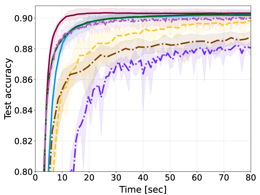
Figure 9: Comparison of the bilevel algorithms on data hyper-cleaning task with mini-batch when $p=0.5$. The training set, the validation set and the test set contain $5000$, $5000$ and $10000$ samples, respectively. The post-fix of legend represents the batch size. Left: test accuracy; Right:test loss.

In the deterministic setting, where we implement all compared methods with full-batch, the training set, the validation set and the test set contain $5000$, $5000$ and $10000$ samples, respectively. For algorithms that incorporate inner iterations to approximate $y^{*}$ or $v^{*}$, we select the inner iteration number from the set $\left\{5i\mid i=1,2,3,4\right\}$. The step size of inner iteration is selected from the set $\{0.01,0.1,1,10\}$ and the step size of outer iteration is chosen from $\left\{5\times 10^{i}\mid i=-3,-2,-1,0,1,2,3\right\}$. The results are presented in Figure 6. Note that LancBiO is crafted for approximating the Hessian inverse vector product $v^{*}$, while the solid methods stocBiO and TTSA are not. Consequently, with respect to the residual norm of the linear system, i.e., $\left\|{A_{k}v_{k}-b_{k}}\right\|$, we only compare the results with AmIGO-GD, AmIGO-CG and SOBA. Observe that the proposed subspace-based LancBiO achieves the lowest residual norm and the best test accuracy, and subBiO is comparable to the other algorithms. Specifically, in Figure 6, the efficiency of LancBiO stems from its accurate approximation of the linear system. Furthermore, we implement the solvers designed for the stochastic setting using mini-batch to enable a broader comparison in Figure 9. It is shown that the stochastic algorithm SOBA tends to converge faster initially, but algorithms employing a full-batch approach achieve higher accuracy.

To explore the potential for extending our proposed methods to a stochastic setting, we also conduct an experiment with stochastic gradients. In this setting, where we implement all compared methods with mini-batch, the training set, the validation set and the test set contain $20000$, $5000$ and $10000$ samples, respectively. For algorithms that incorporate inner iterations to approximate $y^{*}$ or $v^{*}$, we select the inner iteration number from the set $\left\{3i\mid i=1,2,3,4\right\}$. The step size of inner iteration is selected from the set $\{0.01,0.1,1,10\}$, the step size of outer iteration is chosen from $\left\{1\times 10^{i}\mid i=-3,-2,-1,0,1,2,3\right\}$ and the batch size is picked from $\left\{32\times 2^{i}\mid i=0,1,2,3\right\}$. AmIGO-CG is not presented since it fails in this experiment in our setting. The results in Figure 10 demonstrate that LancBiO maintains reasonable performance with stochastic gradients, exhibiting fast convergence rate, although the final convergence accuracy is slightly lower.

Generally, for standard linear systems, the traditional Lanczos process is recognized for its efficiency and versatility over gradient descent methods. LancBiO, in a sense, reflects this principle within the context of bilevel optimization, underscoring the effectiveness of the dynamic Lanczos-aided approach.

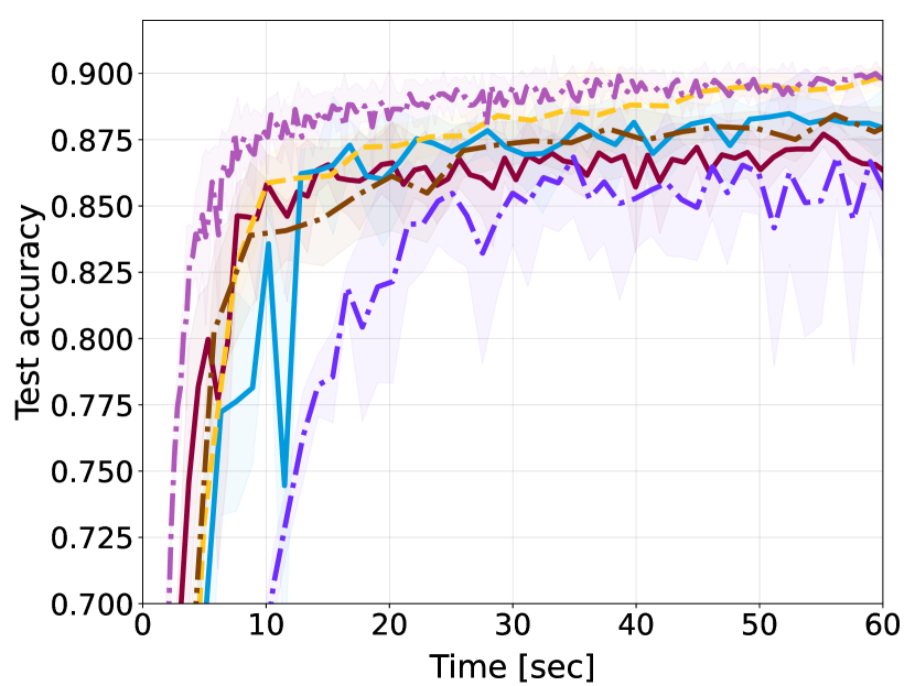
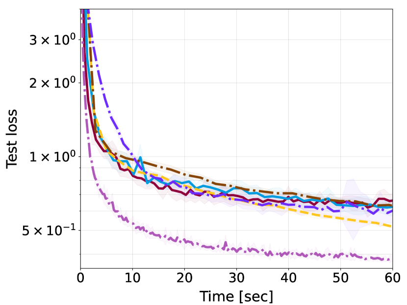
Figure 10: Comparison of the bilevel algorithms on data hyper-cleaning task with mini-batch when $p=0.5$. The training set, the validation set and the test set contain $20000$, $5000$ and $10000$ samples, respectively. The post-fix of legend represents the batch size. Left: test accuracy; Right:test loss.

I.4 Logistic regression on $20$Newsgroup

Consider the hyper-parameters selection task on the $20$Newsgroups dataset (Grazzi et al., 2020), which contains $c=20$ topics with around $18000$ newsgroups posts represented in a feature space of dimension $l=130107$. The goal is to simultaneously train a linear classifier $w$ and determine the optimal regularization parameter $\zeta$. The task is formulated as follows,

$$\begin{array}[]{cl}\min\limits_{\lambda}&\mathcal{L}_{val}(\zeta,w^{*}):=\frac{1}{\left|\mathcal{D}_{\text{val}}\right|}\sum_{(x_{i},y_{i})\in\mathcal{D}_{\text{val}}}L(w^{*}x_{i},y_{i})\\[14.22636pt] \mathrm{s.\,t.}&\begin{aligned} w^{*}&=\operatorname*{arg\,min}_{w}\ \mathcal{L}_{tr}(w,\zeta)\\ :&=\frac{1}{\left|\mathcal{D}_{\text{tr}}\right|}\sum_{(x_{i},y_{i})\in\mathcal{D}_{\text{tr}}}L(wx_{i},y_{i})+\frac{1}{cl}\sum_{i=1}^{c}\sum_{j=1}^{l}\zeta_{j}^{2}w_{ij}^{2}.\end{aligned}\end{array}$$

where $L(\cdot)$ is the cross-entropy loss and $\{\zeta^{2}_{j}\}$ are the non-negative regularizers.

The experiment is implemented in the deterministic setting, where we implement all compared methods with full-batch, the training set, the validation set and the test set contain $5657$, $5657$ and $7532$ samples, respectively. For algorithms that incorporate inner iterations to approximate $y^{*}$ or $v^{*}$, we select the inner iteration number from the set $\left\{5i\mid i=1,2,3,4\right\}$. To guarantee the optimality condition of the lower-level problem, we adopt a decay strategy for the outer iteration step size, i.e., $\lambda_{k}=\lambda/k^{0.4}$, for all algorithms. The constant step size $\theta$ of inner iteration is selected from the set $\{0.01,0.1,1,10\}$ and the initial step size $\lambda$ of outer iteration is chosen from $\left\{5\times 10^{i}\mid i=-3,-2,-1,0,1,2,3\right\}$. The results are presented in Figure 11. In this setting, AmIGO-CG exhibits slightly better performance in reducing the residual norm. Nevertheless, under the same time, LancBiO implements more outer iterations to update $x$, which optimizes the hyper-function more efficiently.

Figure 11: Comparison of the bilevel algorithms hyper-parameters selection task. Left: validation accuracy; Center: validation loss; Right: residual norm of the linear system, $\left\|{A_{k}v_{k}-b_{k}}\right\|$.

References

- Arbel & Mairal (2022) Arbel, M. and Mairal, J. Amortized implicit differentiation for stochastic bilevel optimization. In The Tenth International Conference on Learning Representations, 2022.
- Bellavia & Morini (2001) Bellavia, S. and Morini, B. A globally convergent Newton-GMRES subspace method for systems of nonlinear equations. SIAM Journal on Scientific Computing, 23(3):940–960, 2001.
- Bertinetto et al. (2018) Bertinetto, L., Henriques, J. F., Torr, P. H., and Vedaldi, A. Meta-learning with differentiable closed-form solvers. arXiv preprint arXiv:1805.08136, 2018.
- Brown & Saad (1990) Brown, P. N. and Saad, Y. Hybrid Krylov methods for nonlinear systems of equations. SIAM Journal on Scientific and Statistical Computing, 11(3):450–481, 1990.
- Carmon & Duchi (2018) Carmon, Y. and Duchi, J. C. Analysis of Krylov subspace solutions of regularized non-convex quadratic problems. Advances in Neural Information Processing Systems, 31, 2018.
- Cartis & Roberts (2023) Cartis, C. and Roberts, L. Scalable subspace methods for derivative-free nonlinear least-squares optimization. Mathematical Programming, 199(1-2):461–524, 2023.
- Cartis et al. (2011) Cartis, C., Gould, N. I., and Toint, P. L. Adaptive cubic regularisation methods for unconstrained optimization. part I: motivation, convergence and numerical results. Mathematical Programming, 127(2):245–295, 2011.
- Chakraborty et al. (2023) Chakraborty, S., Bedi, A. S., Koppel, A., Huang, F., and Wang, M. Principal-driven reward design and agent policy alignment via bilevel-rl. In Interactive Learning with Implicit Human Feedback Workshop (ILHF), ICML, 2023.
- Chen et al. (2023) Chen, L., Xu, J., and Zhang, J. On bilevel optimization without lower-level strong convexity. arXiv preprint arXiv:2301.00712, 2023.
- Chen et al. (2021) Chen, T., Sun, Y., and Yin, W. Closing the gap: Tighter analysis of alternating stochastic gradient methods for bilevel problems. In Beygelzimer, A., Dauphin, Y., Liang, P., and Vaughan, J. W. (eds.), Advances in Neural Information Processing Systems, 2021.
- Chen et al. (2022) Chen, T., Sun, Y., Xiao, Q., and Yin, W. A single-timescale method for stochastic bilevel optimization. In International Conference on Artificial Intelligence and Statistics, pp. 2466–2488. PMLR, 2022.
- Dagréou et al. (2022) Dagréou, M., Ablin, P., Vaiter, S., and Moreau, T. A framework for bilevel optimization that enables stochastic and global variance reduction algorithms. Advances in Neural Information Processing Systems, 35:26698–26710, 2022.
- Dempe & Dutta (2012) Dempe, S. and Dutta, J. Is bilevel programming a special case of a mathematical program with complementarity constraints? Mathematical programming, 131:37–48, 2012.
- Dempe & Zemkoho (2013) Dempe, S. and Zemkoho, A. B. The bilevel programming problem: reformulations, constraint qualifications and optimality conditions. Mathematical Programming, 138:447–473, 2013.
- Franceschi et al. (2017) Franceschi, L., Donini, M., Frasconi, P., and Pontil, M. Forward and reverse gradient-based hyperparameter optimization. In International Conference on Machine Learning, pp. 1165–1173. PMLR, 2017.
- Franceschi et al. (2018) Franceschi, L., Frasconi, P., Salzo, S., Grazzi, R., and Pontil, M. Bilevel programming for hyperparameter optimization and meta-learning. In International conference on machine learning, pp. 1568–1577. PMLR, 2018.
- Gao et al. (2023) Gao, W., Qu, Z., Udell, M., and Ye, Y. Scalable approximate optimal diagonal preconditioning. arXiv preprint arXiv:2312.15594, 2023.
- Ghadimi & Wang (2018) Ghadimi, S. and Wang, M. Approximation methods for bilevel programming. arXiv preprint arXiv:1802.02246, 2018.
- Golub & Van Loan (2013) Golub, G. H. and Van Loan, C. F. Matrix computations. JHU press, 2013.
- Gould et al. (1999) Gould, N. I., Lucidi, S., Roma, M., and Toint, P. L. Solving the trust-region subproblem using the Lanczos method. SIAM Journal on Optimization, 9(2):504–525, 1999.
- Grazzi et al. (2020) Grazzi, R., Franceschi, L., Pontil, M., and Salzo, S. On the iteration complexity of hypergradient computation. In International Conference on Machine Learning, pp. 3748–3758. PMLR, 2020.
- Greenbaum (1997) Greenbaum, A. Iterative methods for solving linear systems. SIAM, 1997.
- Greenbaum et al. (1999) Greenbaum, A., Druskin, V., and Knizhnerman, L. On solving indefinite symmetric linear systems by means of the Lanczos method. Comput. Math. Math. Phys, 39(3):350–356, 1999.
- Hao et al. (2024) Hao, J., Gong, X., and Liu, M. Bilevel optimization under unbounded smoothness: A new algorithm and convergence analysis. In The Twelfth International Conference on Learning Representations, 2024.
- Hestenes et al. (1952) Hestenes, M. R., Stiefel, E., et al. Methods of conjugate gradients for solving linear systems. Journal of research of the National Bureau of Standards, 49(6):409–436, 1952.
- Hong et al. (2023) Hong, M., Wai, H.-T., Wang, Z., and Yang, Z. A two-timescale stochastic algorithm framework for bilevel optimization: Complexity analysis and application to actor-critic. SIAM Journal on Optimization, 33(1):147–180, 2023.
- Hu et al. (2023) Hu, X., Xiao, N., Liu, X., and Toh, K.-C. An improved unconstrained approach for bilevel optimization. SIAM Journal on Optimization, 33(4):2801–2829, 2023.
- Ji et al. (2021) Ji, K., Yang, J., and Liang, Y. Bilevel optimization: Convergence analysis and enhanced design. In International conference on machine learning, pp. 4882–4892. PMLR, 2021.
- Ji et al. (2022) Ji, K., Liu, M., Liang, Y., and Ying, L. Will bilevel optimizers benefit from loops. Advances in Neural Information Processing Systems, 35:3011–3023, 2022.
- Jiang et al. (2024) Jiang, R., Raman, P., Sabach, S., Mokhtari, A., Hong, M., and Cevher, V. Krylov cubic regularized newton: A subspace second-order method with dimension-free convergence rate. arXiv preprint arXiv:2401.03058, 2024.
- Khanduri et al. (2021) Khanduri, P., Zeng, S., Hong, M., Wai, H.-T., Wang, Z., and Yang, Z. A near-optimal algorithm for stochastic bilevel optimization via double-momentum. Advances in neural information processing systems, 34:30271–30283, 2021.
- Krylov (1931) Krylov, A. N. On the numerical solution of the equation by which in technical questions frequencies of small oscillations of material systems are determined. Izvestija AN SSSR (News of Academy of Sciences of the USSR), Otdel. mat. i estest. nauk, 7(4):491–539, 1931.
- Kuczyński & Woźniakowski (1992) Kuczyński, J. and Woźniakowski, H. Estimating the largest eigenvalue by the power and Lanczos algorithms with a random start. SIAM journal on matrix analysis and applications, 13(4):1094–1122, 1992.
- Kwon et al. (2023a) Kwon, J., Kwon, D., Wright, S., and Nowak, R. On penalty methods for nonconvex bilevel optimization and first-order stochastic approximation. arXiv preprint arXiv:2309.01753, 2023a.
- Kwon et al. (2023b) Kwon, J., Kwon, D., Wright, S., and Nowak, R. D. A fully first-order method for stochastic bilevel optimization. In International Conference on Machine Learning, pp. 18083–18113. PMLR, 2023b.
- Lanczos (1950) Lanczos, C. An iteration method for the solution of the eigenvalue problem of linear differential and integral operators. Journal of Research of the National Bureau of Standards, 45(4), 1950.
- LeCun et al. (1998) LeCun, Y., Bottou, L., Bengio, Y., and Haffner, P. Gradient-based learning applied to document recognition. Proceedings of the IEEE, 86(11):2278–2324, 1998.
- Li et al. (2022) Li, J., Gu, B., and Huang, H. A fully single loop algorithm for bilevel optimization without Hessian inverse. In Proceedings of the AAAI Conference on Artificial Intelligence, volume 36, pp. 7426–7434, 2022.
- Li et al. (2020) Li, Y., Liu, H., Wen, Z., and Yuan, Y.-x. Low-rank matrix iteration using polynomial-filtered subspace extraction. SIAM Journal on Scientific Computing, 42(3):A1686–A1713, 2020. doi: 10.1137/19M1259444.
- Li et al. (2023) Li, Y., Lin, G.-H., Zhang, J., and Zhu, X. A novel approach for bilevel programs based on Wolfe duality. arXiv preprint arXiv:2302.06838, 2023.
- Lin et al. (2014) Lin, G.-H., Xu, M., and Ye, J. J. On solving simple bilevel programs with a nonconvex lower level program. Mathematical Programming, 144(1-2):277–305, 2014.
- Liu et al. (2022) Liu, B., Ye, M., Wright, S., Stone, P., and Liu, Q. Bome! bilevel optimization made easy: A simple first-order approach. Advances in Neural Information Processing Systems, 35:17248–17262, 2022.
- Liu et al. (2018) Liu, H., Simonyan, K., and Yang, Y. Darts: Differentiable architecture search. arXiv preprint arXiv:1806.09055, 2018.
- Liu et al. (2020) Liu, R., Mu, P., Yuan, X., Zeng, S., and Zhang, J. A generic first-order algorithmic framework for bi-level programming beyond lower-level singleton. In International Conference on Machine Learning, pp. 6305–6315. PMLR, 2020.
- Liu et al. (2023) Liu, R., Liu, Y., Yao, W., Zeng, S., and Zhang, J. Averaged method of multipliers for bi-level optimization without lower-level strong convexity. In Proceedings of the 40th International Conference on Machine Learning, volume 202 of Proceedings of Machine Learning Research, pp. 21839–21866. PMLR, 23–29 Jul 2023.
- Liu et al. (2013) Liu, X., Wen, Z., and Zhang, Y. Limited memory block Krylov subspace optimization for computing dominant singular value decompositions. SIAM Journal on Scientific Computing, 35(3):A1641–A1668, 2013.
- Liu et al. (2021) Liu, X., Wen, Z., and Yuan, Y.-X. Subspace methods for nonlinear optimization. CSIAM Trans. Appl. Math, 2(4):585–651, 2021.
- Lu & Mei (2023) Lu, Z. and Mei, S. First-order penalty methods for bilevel optimization. arXiv preprint arXiv:2301.01716, 2023.
- Maclaurin et al. (2015) Maclaurin, D., Duvenaud, D., and Adams, R. Gradient-based hyperparameter optimization through reversible learning. In International conference on machine learning, pp. 2113–2122. PMLR, 2015.
- Meurant & Strakoš (2006) Meurant, G. and Strakoš, Z. The Lanczos and conjugate gradient algorithms in finite precision arithmetic. Acta Numerica, 15:471–542, 2006.
- Nesterov et al. (2018) Nesterov, Y. et al. Lectures on convex optimization, volume 137. Springer, 2018.
- Outrata (1990) Outrata, J. V. On the numerical solution of a class of Stackelberg problems. Zeitschrift für Operations Research, 34:255–277, 1990.
- Paige (1971) Paige, C. C. The computation of eigenvalues and eigenvectors of very large sparse matrices. PhD thesis, University of London, 1971.
- Paige (1976) Paige, C. C. Error analysis of the lanczos algorithm for tridiagonalizing a symmetric matrix. IMA Journal of Applied Mathematics, 18(3):341–349, 1976.
- Paige (1980) Paige, C. C. Accuracy and effectiveness of the Lanczos algorithm for the symmetric eigenproblem. Linear algebra and its applications, 34:235–258, 1980.
- Paige & Saunders (1975) Paige, C. C. and Saunders, M. A. Solution of sparse indefinite systems of linear equations. SIAM journal on numerical analysis, 12(4):617–629, 1975.
- Parlett (1998) Parlett, B. N. The symmetric eigenvalue problem. SIAM, 1998.
- Pedregosa (2016) Pedregosa, F. Hyperparameter optimization with approximate gradient. In International conference on machine learning, pp. 737–746. PMLR, 2016.
- Ramzi et al. (2022) Ramzi, Z., Mannel, F., Bai, S., Starck, J.-L., Ciuciu, P., and Moreau, T. Shine: Sharing the inverse estimate from the forward pass for bi-level optimization and implicit models. In International Conference on Learning Representations, 2022.
- Saad (2011) Saad, Y. Numerical methods for large eigenvalue problems. SIAM, 2011.
- Shaban et al. (2019) Shaban, A., Cheng, C.-A., Hatch, N., and Boots, B. Truncated back-propagation for bilevel optimization. In The 22nd International Conference on Artificial Intelligence and Statistics, pp. 1723–1732. PMLR, 2019.
- Stackelberg (1952) Stackelberg, H. v. The theory of the market economy. Oxford University Press, 1952.
- Wang et al. (2021) Wang, J., Chen, H., Jiang, R., Li, X., and Li, Z. Fast algorithms for Stackelberg prediction game with least squares loss. In International Conference on Machine Learning, pp. 10708–10716. PMLR, 2021.
- Wang et al. (2022) Wang, X., Guo, W., Su, J., Yang, X., and Yan, J. Zarts: On zero-order optimization for neural architecture search. Advances in Neural Information Processing Systems, 35:12868–12880, 2022.
- Xiao et al. (2023) Xiao, Q., Lu, S., and Chen, T. An alternating optimization method for bilevel problems under the Polyak-łojasiewicz condition. In Annual Conference on Neural Information Processing Systems, 2023.
- Xu & Ye (2014) Xu, M. and Ye, J. J. A smoothing augmented Lagrangian method for solving simple bilevel programs. Computational Optimization and Applications, 59:353–377, 2014.
- Yang et al. (2023) Yang, H., Luo, L., Li, C. J., Jordan, M., and Fazel, M. Accelerating inexact hypergradient descent for bilevel optimization. In OPT 2023: Optimization for Machine Learning, 2023.
- Ye & Zhu (1995) Ye, J. J. and Zhu, D. Optimality conditions for bilevel programming problems. Optimization, 33(1):9–27, 1995.
- Ye & Zhu (2010) Ye, J. J. and Zhu, D. New necessary optimality conditions for bilevel programs by combining the MPEC and value function approaches. SIAM Journal on Optimization, 20(4):1885–1905, 2010.
- Yuan (2014) Yuan, Y.-x. A review on subspace methods for nonlinear optimization. In Proceedings of the International Congress of Mathematics, pp. 807–827, 2014.
- Zhang et al. (2017) Zhang, L.-H., Shen, C., and Li, R.-C. On the generalized Lanczos trust-region method. SIAM Journal on Optimization, 27(3):2110–2142, 2017.
- Zhang et al. (2023) Zhang, Y., Khanduri, P., Tsaknakis, I., Yao, Y., Hong, M., and Liu, S. An introduction to bi-level optimization: Foundations and applications in signal processing and machine learning. arXiv preprint arXiv:2308.00788, 2023.