A classification of well-behaved graph clustering schemes

Abstract

Community detection in graphs is a problem that is likely to be relevant whenever network data appears, and consequently the problem has received much attention with many different methods and algorithms applied. However, many of these methods are hard to study theoretically, and they optimise for somewhat different goals. A general and rigorous account of the problem and possible methods remains elusive.

We study the class of all clustering methods that are monotone under addition of vertices and edges, phrasing this as a functoriality notion. We show that if additionally we require the methods to have no resolution limit in a strong sense, this is equivalent to a notion of representability, which requires them to be explainable and determined by a representing set of graphs. We show that representable clustering methods are always computable in polynomial time, and in any nowhere dense class they are computable in roughly quadratic time.

Finally, we extend our definitions to the case of hierarchical clustering, and give a notion of representability for hierarchical clustering schemes.

1 Introduction

The problem of inferring community structure from a graph is one that appears in many different guises in different research areas. It is useful for everything from assigning research papers to subfields of physics [CR10], assessing the development of nano-medicine by studying patent cocitation networks [BAB12], studying brain function via the community structure of the connectome [Bet23], understanding how different bird species spread various plant seeds [Cos+16], to studying hate speech on Twitter [Evk+21].

Despite, or perhaps because of, the widespread nature of this problem, there is no universally agreed on definition of what is actually meant by community structure. This leads to varying methods being used to solve the problem, that do not necessarily give the same results. One of the most popular definitions in practice is the modularity of a partition, introduced by Newman and Girvan [NG04] – it is the method used in all the examples given in the previous paragraph. There are however many other methods, such as the flow-based infomap method motivated by information theory [RAB09], more statistically sound methods assuming a generative model [Pei14], novel graph neural network methods [Koj+23], and many more [Jav+18].

One thing nearly all of these methods have in common is that they are in a sense black boxes – they do not give you any way of answering the question of why two vertices were put in the same part. They are also generally hard to study in a rigorous mathematical way, resulting in few theoretical guarantees for their behaviour. While modularity has proven itself very useful in practice, it is in fact guaranteed to behave in undesirable ways in certain settings.

In particular, modularity suffers from a “resolution limit”, wherein it cannot “see” things happening in subgraphs that are small compared to the total graph, resulting in very unexpected behaviour [FB07]. In Figure 1 we see one illustration of this phenomenon – one would hope that what happens in one connected component cannot affect the other, but the resolution limit results in this undesirable behaviour.

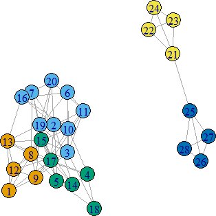
(a) A graph $G$, with vertices coloured according to the modularity-maximising partition

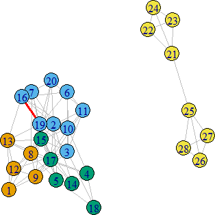
(b) $G$ with a single edge added, highlighted in red, and its new optimal partition

Figure 1: An illustration of the resolution limit issue with modularity.

Another issue with studying modularity optimization from a theoretical perspective is the fact that computing it is NP-hard [Bra+08]. This means that when using modularity maximization in practice, one always needs a heuristic algorithm for finding good partitions, such as the Louvain [Blo+08] or Leiden [TWV19] algorithms, which themselves do not have many known theoretical guarantees connecting them to modularity. Thus, one is left having to either study modularity itself, and hoping that the results say something about the results of these algorithms, or studying the algorithms themselves, and not directly saying anything about modularity.

These issues with the varying optimization based approaches to clustering lead us to investigating a more “axiomatic” approach to the problem – that is, we want to specify a few properties that the clustering method must have, and then see what methods there are that satisfy these properties. Other than of course giving us guarantees on the behaviour of our methods, this approach also gives us much more straightforward algorithms which run in polynomial time, since we are no longer doing optimization, but in some sense just applying a decision rule for when vertices should be in the same part or not.

Our particular approach to this is motivated by the results of Carlsson and Mémoli [CM13] for the analogous problem of clustering finite metric spaces. Like in their setting, there are three properties that are of interest:

1. Functoriality is essentially a form of monotonicity under addition of edges or vertices to the graph. Adding a new edge or new vertex should only ever make communities more closely connected, it should never split them.

2. Excisiveness is a very strict version of requiring that there be no resolution limit – instead we require that the method be idempotent on the parts it has found. That is, if we take some graph $G$, cluster it, and then look at the subgraph induced by any part, that graph has to be clustered into just a single large component, so we never discover new features at smaller scales.

3. Representability is a type of explainability of the clustering method. A representable clustering method $F_{\Omega}$ is determined by a set $\Omega$ of simple graphs, and the rule that two vertices of a graph $G$ will be in the same part if their neighbourhood looks like something in $\Omega$. This also gives us a simple algorithm to actually compute the partitioning of a graph, that runs in polynomial time for each fixed $\Omega$.

Our main result classifies exactly the relationship between these properties, and shows that all representable clustering schemes are tractable on a large class of sparse graphs:

Theorem 1.1 (Main results).

A clustering scheme is representable if and only if it is excisive and functorial. Further, any such representable clustering scheme is computable in quadratic time on any graph class of bounded expansion.

We also give a structural result for when two representable clustering schemes are equal, and use this to prove that there exist representable clustering schemes that are not finitely representable. Finally, we extend our definition of a representable clustering scheme into the setting of hierarchical clustering schemes. Here, instead of just assigning a single clustering to each graph, we give one clustering for each “scale”, giving a spectrum of clusterings of the graph from coarsest to finest. In this setting, we find that the connection to excisiveness no longer works.

2 Definitions of our terms

Definition 2.1.

The category of simple graphs ${\mathcal{G}}$ has as its objects simple graphs, which we consider to be a finite set $V$ equipped with a reflexive and symmetric binary relation $E$ – that is, our simple graphs are finite, have no double edges, and have loops at every vertex. A morphism from $H=(V,E)$ to $G=(V^{\prime},E^{\prime})$ is an injective set function $f:V\to V^{\prime}$ such that whenever $uEv$, we also have $f(u)E^{\prime}f(v)$. That is, a morphism from $H$ to $G$ is a way of realising $H$ as a subgraph of $G$.

Definition 2.2.

The category of partitioned sets $\mathcal{P}$ has as its objects finite sets $V$ with an equivalence relation $\sim$. A morphism in $\mathcal{P}$ from $(V,\sim)$ to $(W,\approx)$ is a set function $f:V\to W$ such that whenever $v\sim w$, $f(v)\approx f(w)$.

Definition 2.3.

A clustering scheme is a function $\mathfrak{C}$ that sends simple graphs to partitioned sets, with the same underlying set – that is, if $\mathfrak{C}$ sends $G=(V,E)$ to $P=(W,\sim)$, we require that $V=W$. We say that it is functorial if it is a functor from ${\mathcal{G}}$ to $\mathcal{P}$.

One good way to think of these definitions is as a kind of generalization of monotonicity. If we were restricting to only studying clustering of graphs on a fixed underlying set, the statement that there is a morphism from $G$ to $H$ becomes precisely the statement that $G\subseteq H$, that is that $G$ is less than $H$ in the inclusion order. Likewise there is a natural partial order on the set of equivalence relations on the underlying vertex set, given by that $\sim<\approx$ if $\sim$ is a refinement of $\approx$, or equivalently if $\approx$ is a coarsening of $\sim$.

In this restricted setting, the statement that a clustering scheme is functorial becomes exactly the statement that it is monotone with respect to the inclusion order and the order on equivalence relations. By using the language of category theory to encode this information, we gain the ability to talk about things being “monotone under addition of vertices”, not just under addition of edges.

Definition 2.4.

A clustering scheme $\mathfrak{C}$ is excisive if, for all graphs $G=(V,E)$, it holds for every equivalence class $A$ of $\mathfrak{C}(G)$ that $\mathfrak{C}$ sends $G|_{A}$, the subgraph of $G$ induced by $A$, to $(A,\sim_{\text{cpl}})$, where $\sim_{\text{cpl}}$ is the complete equivalence relation that declares all objects in $A$ equivalent.

That is, if we take a graph, cluster it, pick out one of the parts, and cluster that part alone, that part will be clustered into a single part.

3 Representability

Definition 3.1.

Given a not necessarily finite set $\Omega$ of simple graphs, we define the endofunctor $F_{\Omega}$ on ${\mathcal{G}}$ as follows: For any graph $G=(V,E)$, $F_{\Omega}(G)$ is a graph on the same vertex set, and there is an edge between $u$ and $v$ in $F_{\Omega}(G)$ whenever there exists some subgraph of $G$ containing both $u$ and $v$ which is isomorphic to some $\omega\in\Omega$.

Equivalently, there is an edge $uv$ in $F_{\Omega}(G)$ whenever there exists an $\omega\in\Omega$ and a morphism $f:\omega\to G$ such that $f(\omega)\ni u,v$.

On morphisms, $F_{\Omega}$ is always just the identity.

That this definition does in fact always give us a functor is something that needs to be checked – it is not immediate from the definition, even though we said in the definition that it is an endofunctor.

Lemma 3.2.

For any representing set $\Omega$ of simple graphs, $F_{\Omega}$ is indeed an endofunctor on ${\mathcal{G}}$.

Proof.

That it always gives a simple graph and that it respects identity morphisms and composition of morphisms is easy to see. The only thing we actually need to check is that if $f:H\to G$ is a morphism, then $F_{\Omega}(f)=f:F_{\Omega}(H)\to F_{\Omega}(G)$ is also a morphism.

Unwrapping this statement, what we need is that, for any morphism $f:H\to G$, whenever $uv$ is an edge in $F_{\Omega}(H)$, $f(u)f(v)$ is an edge in $F_{\Omega}(G)$. Now, that $uv$ is an edge in $F_{\Omega}(H)$ means that there is an $\omega\in\Omega$ and $f_{\omega}:\omega\to H$ such that $f(\omega)\ni u,v$.

But consider what happens if we just compose $f_{\omega}$ and $f$ – this will be a morphism from $\omega$ into $G$, and trivially we must have that $f(f_{\omega}(\omega))\ni f(u),f(v)$, and so there must be an edge $f(u)f(v)$ in $F_{\Omega}(G)$, by definition of $F_{\Omega}$. ∎

What is going on in the proof of Lemma 3.2 is much clearer if we just think about it in terms of things being subgraphs of each other, forgetting the data of how exactly they are subgraphs. Then the statement that $F_{\Omega}$ is a functor boils down to the statement that if $\omega$ is a subgraph of $H$ and $H$ is a subgraph of $G$, then certainly $\omega$ is a subgraph of $G$, and so $F_{\Omega}(G)$ must have all the edges $F_{\Omega}(H)$ has, since edges in $F_{\Omega}(G)$ represent the presence of a certain subgraph in $G$.

Definition 3.3.

The functor $\Pi:{\mathcal{G}}\to\mathcal{P}$ which sends a graph to its partition into connected components is called the connected components functor. Equivalently, we can think of this functor as finding the least equivalence relation that contains the relation $E$ defining the edges, where we by “least” mean least in the subset relation.

Definition 3.4.

A clustering scheme $\mathfrak{C}$ is representable if $\mathfrak{C}=F_{\Omega}\circ\Pi$ for some representable endofunctor $F_{\Omega}$. Notice that this means that all representable clustering schemes are functorial, being the composition of two functors.

Example 3.5.

The connected components functor is representable, with representing set $\Omega=\{K_{2}\}$. In fact any set $\Omega$ of connected graphs containing $K_{2}$ will represent the connected components functor – but note that they will in general give inequivalent endofunctors on ${\mathcal{G}}$.

One somewhat surprising fact is that there are actually representable clustering schemes that are not finitely representable.

Theorem 3.6.

There exists a representable clustering scheme $F_{\Omega}\circ\Pi$ which is not finitely representable, that is, it is not equal to $F_{\Gamma}\circ\Pi$ for any finite set of simple graphs $\Gamma$.

In order to give a proof of this, we first need a structural result about how these endofunctors behave.

Remark 3.7.

For any $\omega\in\Omega$, it is trivial to see that $F_{\Omega}(\omega)$ must be a clique, since we can just take the identity morphism on $\omega$ to show that all edges must exist.

In fact, which graphs are sent to cliques by $F_{\Omega}$ essentially determines what it does as a functor. Similarly, if we are interested in the weaker equivalence of inducing the same clustering scheme, this is determined by which graphs are sent to a connected graph.

Lemma 3.8.

For any set $\Omega$ of simple graphs and any simple graph $G=(V,E)$, it holds that $F_{\Omega\cup\{G\}}=F_{\Omega}$ if and only if $F_{\Omega}(G)=(V,V^{2})$, that is, if $G$ is sent to a clique on its vertices by $F_{\Omega}$.

Proof.

Suppose $F_{\Omega\cup\{G\}}=F_{\Omega}$. That $F_{\Omega\cup\{G\}}(G)=(V,V^{2})$ is immediate by Remark 3.7, and so since $F_{\Omega\cup\{G\}}=F_{\Omega}$, we also have $F_{\Omega}(G)=(V,V^{2})$, as desired.

Now suppose $F_{\Omega}(G)=(V,V^{2})$, and let $H$ be some arbitrary simple graph. We wish to show that $F_{\Omega\cup\{G\}}(H)=F_{\Omega}(H)$.

That edges of $F_{\Omega}(H)$ must also be edges of $F_{\Omega\cup\{G\}}(H)$ is obvious, so all we need to show is that edges of $F_{\Omega\cup\{G\}}(H)$ are also edges of $F_{\Omega}(H)$. Thus, suppose $uv$ is an edge of $F_{\Omega\cup\{G\}}(H)$ – that this edge exists must be because there is some $\omega\in\Omega\cup\{G\}$ and an $f:\omega\to H$ such that $f(\omega)\ni u,v$.

If this $\omega$ is not $G$, then we are done. If it is $G$, we recall that since $F_{\Omega}(G)$ is a clique, there must be an edge $f^{-1}(u)f^{-1}(v)$ in it. Therefore there must exist some $\omega\in\Omega$ and some $g:\omega\to G$ such that $f(\omega)\ni f^{-1}(u),f^{-1}(v)$. But then the composition $g\circ f:\omega\to H$ will be a morphism from an $\omega\in\Omega$ into $H$ whose image contains $u$ and $v$, proving that $uv$ is an edge of $F_{\Omega}(H)$. ∎

Lemma 3.9.

For any set of simple graphs $\Omega$ and any simple graph $G$, $\Omega$ and $\Omega\cup\{G\}$ induce the same representable clustering scheme if and only if $F_{\Omega}(G)$ is a connected graph.

Proof.

Suppose $\Omega$ and $\Omega\cup\{G\}$ induce the same clustering scheme, that is, that $F_{\Omega}\circ\Pi=F_{\Omega\cup\{G\}}\circ\Pi$. What we need to show is that $F_{\Omega}(G)$ is connected – which is the same thing as showing that $(F_{\Omega}\circ\Pi)(G)$ is a clique. By assumption $F_{\Omega}\circ\Pi=F_{\Omega\cup\{G\}}\circ\Pi$, so it suffices to show that $(F_{\Omega\cup\{G\}}\circ\Pi)(G)$ is a clique. This, however, is immediate by Remark 3.7, since it gives us that already $F_{\Omega\cup\{G\}}(G)$ is a clique.

For the other direction, assume that $F_{\Omega}(G)$ is connected. To show that $\Omega$ and $\Omega\cup\{G\}$ induce equivalent clustering schemes, it is sufficient to show that for every graph $H$, $F_{\Omega}(H)$ and $F_{\Omega\cup\{G\}}(H)$ have the same partition into connected components.

First observe, as we did in the proof of Lemma 3.8, that in fact $F_{\Omega}(H)$ is a subgraph of $F_{\Omega\cup\{G\}}$, so it suffices to show that whenever there is a path connecting $u$ and $v$ in $F_{\Omega\cup\{G\}}(H)$, there is already such a path in $F_{\Omega}(H)$.

To show this, we show that whenever there is an edge between $u$ and $v$ in $F_{\Omega\cup\{G\}}(H)$, there is a path between $u$ and $v$ in $F_{\Omega}(H)$.

Now, this edge between $u$ and $v$ has to be created by some $\omega\in\Omega$ and a morphism $f:\omega\to H$ such that $\operatorname{im}f\ni u,v$. If this $\omega$ is not $G$, we are already done, so suppose it is $G$.

Let $v^{\prime}=f^{-1}(v)$ and $u^{\prime}=f^{-1}(u)$. Since $F_{\Omega}(G)$ is by assumption connected, it contains a path $v^{\prime}e_{1}w_{1}e_{2}\ldots w_{k}e_{k}u^{\prime}$. Each of the edges $e_{i}$ is created by an $\omega_{i}\in\Omega$ and $f_{i}:\omega_{i}\to G$ such that $\operatorname{im}f_{i}\ni w_{i-1},w_{i}$.

If we just compose these $f_{i}$s with $f$ we get functions from $\omega_{i}\in\Omega$ into $H$ whose images contain $f(w_{i})$, so we get edges between these $f(w_{i})$s, and so we get a path between them, which will be precisely a path connecting $u$ and $v$. ∎

With this result in hand, we can now give a proof of the existence of a representable but not finitely representable endofunctor.

Proof of Theorem 3.6.

Let, for each $i$, $\omega_{i}$ consist of a triangle with a tail of $i$ vertices, as shown in Figure 2, and let $\Omega=\left\{\omega_{i}\ \middle|\ i\in{\mathbb{N}}\right\}$. We claim that $F_{\Omega}$ is not equal to $F_{\Gamma}$ for any finite set of simple graphs $\Gamma$.

Figure 2: The family of graphs $\{\omega_{i}\}_{i=0}^{3}$.

To prove this, let us first define

$$\bar{\Omega}=\left\{G\in{\mathcal{G}}\ \middle|\ F_{\Omega}(G)\text{ is connected.}\right\}$$

as the set of all graphs which $F_{\Omega}$ sends to connected graphs. By Lemma 3.9, $F_{\Omega}=F_{\bar{\Omega}}$, and $\bar{\Omega}$ is the greatest set with this property.

A little bit of reflection will make it clear that $\bar{\Omega}$ is precisely the set of connected graphs which contain a triangle. Particularly, for any edge in such a graph, we can map the tail end of some $\omega_{i}$ onto that edge, the rest of the tail onto a path to the triangle in the graph, and the triangle of the $\omega_{i}$ onto the triangle of the graph. That $F_{\Omega}$ will send any triangle-free graph to a graph with no edges is clear, since there is no morphism from any triangle-containing graph such as $\omega_{i}$ into a triangle-free graph. Likewise, that it cannot send a disconnected graph to a connected graph is immediate from that $\Omega$ contains only connected graphs.

Now suppose for contradiction that $\Gamma$ is a finite set of graphs such that $F_{\Gamma}=F_{\bar{\Omega}}$. Lemma 3.9 implies that we must have $\Gamma\subset\bar{\Omega}$, since if there were a $\gamma\in\Gamma\setminus\bar{\Omega}$ it’d be sent to a connected graph by $F_{\Gamma}$, and thus also by $F_{\bar{\Omega}}$, since we’ve assumed they are equal – but we chose $\bar{\Omega}$ so that it already contains everything sent to a connected graph by $F_{\bar{\Omega}}$.

So, let

$$\delta=\max_{\gamma\in\Gamma}\max_{u\in V_{\gamma}}\min_{\begin{subarray}{c}v\in V_{\gamma}\\ v\text{ is in a triangle}\end{subarray}}d(u,v).$$

That is, $\delta$ is the furthest any vertex in any graph in $\Gamma$ is from a triangle. We claim that $F_{\Gamma}$ will not send $\omega_{\delta+1}$ to a connected graph, proving it is not equal to $F_{\bar{\Omega}}$, giving our contradiction.

That this is so is actually easy to see – if $\omega_{\delta+1}$ were sent to a connected graph, that must in particular mean there is an edge in $F_{\Gamma}(\omega_{\delta+1})$ between the tail vertex and its neighbour. So there is some morphism from some $\gamma\in\Gamma$ that hits both vertices. However, such a morphism must also map the triangle in $\gamma$ onto the triangle in $\omega_{\delta+1}$, since that is the only place the triangle can go. Then, however, it cannot also reach to the tail – the tail is further away from the triangle than any vertex in any $\gamma$ is from the triangle. Thus, no such morphism can exist, and we are done. ∎

Remark 3.10.

The construction in our proof of course works equally as well replacing the triangle by any connected graph that is not a line. So we have found a large family of examples of classes of graphs that give representable but not finitely representable endofunctors.

The question of which natural classes of graphs are representable or finitely representable may be interesting. The connected graphs, for example, are of course represented by just a $K_{2}$. The example we gave in the proof easily generalises to showing that the graphs of girth at most $k$ are representable but not finitely representable, by extending from triangles with tails to all cycles of length at most $k$ with tails.

The class of non-planar graphs is also representable, with itself as a representation, since there can of course be no morphism from a non-planar graph into a planar graph. Wagner’s theorem tells us that we could also pick the set of all graphs formed from $K_{3,3}$ or $K_{5}$ by replacing edges with paths as our representing set for non-planar graphs. Whether there exists a smaller or even finite representing set is a potentially interesting question, which we leave unanswered.

4 Equivalence of representability and excisiveness

We are able to exactly characterise the relationship between the three concepts of functoriality, representability, and excisiveness for clustering schemes.

Theorem 4.1.

A clustering scheme is representable if and only if it is excisive and functorial. No other implications hold between these concepts.

We divide the proof of Theorem 4.1 into two lemmas and a collection of examples, as illustrated in Figure 3. We have already seen from Lemma 3.2 that representability implies functoriality, so it remains to see that it also implies excisiveness, and then to show the necessity of the condition.

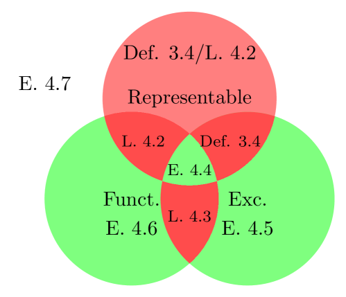
Figure 3: A Venn diagram illustrating the structure of the proof of Theorem 4.1. Impossible combinations of properties are in red, possible ones (other than having no property) are in green, and the labels indicate the lemma or example proving the intersection is empty or non-empty.

Lemma 4.2.

A representable clustering scheme is excisive.

Proof.

Let $\Omega$ be some set of simple graphs, and $G$ be some simple graph. Assume the equivalence classes of $(F_{\Omega}\circ\Pi)(G)$ are $\{A_{1},A_{2},\ldots A_{k}\}$, and let $H=G|_{A_{1}}$ be the induced subgraph of $G$ on $A_{1}$. What we need to show is that $(F_{\Omega}\circ\Pi)(H)=(A_{1},\sim_{\text{cpl}})$, that is, that every vertex is equivalent in the clustering of $H$.

It is obvious that this is equivalent to showing that $F_{\Omega}(H)$ is a connected graph. We will in fact show something stronger – that $F_{\Omega}(H)=F_{\Omega}(G|_{A_{1}})=(F_{\Omega}(G))|_{A_{1}}$. Since $A_{1}$ is an equivalence class of $F_{\Omega}\circ\Pi$, it must be a connected component of $F_{\Omega}(G)$, and so this will show what we want.

First, let $f:H\hookrightarrow G$ be the subgraph inclusion morphism of $H$ into $G$. By functoriality of $F_{\Omega}$, $f$ is also a morphism from $F_{\Omega}(H)$ into $F_{\Omega}(G)$, showing that $F_{\Omega}(H)$ is a subgraph of $F_{\Omega}(G)$, so every edge of $F_{\Omega}(H)$ is an edge of $F_{\Omega}(G)$

Now, let $uv$ be an arbitrary edge of $F_{\Omega}(G)|_{A_{1}}$. We wish to show this is already an edge of $F_{\Omega}(H)$. That it is an edge of $F_{\Omega}(G)$ means there exists some $\omega\in\Omega$ and a morphism $f_{\omega}:\omega\to G$ such that $\operatorname{im}(f_{\omega})\ni u,v$.

We claim that in fact $\operatorname{im}(f_{\omega})\subset A_{1}$, so that $f_{\omega}$ restricts to a morphism into $H$. If we can show this, this will show that there is an edge $uv$ also in $F_{\Omega}(H)$, and we will be done.

Let $w$ be an arbitrary vertex in $\operatorname{im}(f_{\omega})$. Now $f_{\omega}$ is also a morphism from something in $\Omega$ that hits both $w$ and $v$, so there is an edge $vw$ in $F_{\Omega}(G)$. But this of course means that $w$ and $v$ are in the same connected component – and this connected component is precisely $A_{1}$. Thus, $w\in A_{1}$, and we are done. ∎

Lemma 4.3.

An excisive and functorial clustering scheme is representable.

Proof.

Let $\mathfrak{C}$ be some excisive and functorial clustering scheme, and let

$$\Omega=\left\{G\in{\mathcal{G}}\ \middle|\ \mathfrak{C}(G)=(V_{G},\sim_{\text{cpl}})\right\},$$

that is, $\Omega$ is the set of all graphs clustered by $\mathfrak{C}$ into a single part. We will show that in fact $\mathfrak{C}=F_{\Omega}$.

So, let $G$ be some graph. We need to show two things:

1. Whenever $u$ and $v$ are clustered in the same part by $\mathfrak{C}$, they are in the same connected component of $F_{\Omega}(G)$.

2. Whenever $uv$ is an edge of $F_{\Omega}(G)$, $u$ and $v$ are clustered in the same part by $\mathfrak{C}$. This of course implies that whenever $u$ and $v$ are in the same connected component, they are also clustered in the same part by $\mathfrak{C}$, which is what we really need.

We start with the first direction, letting $u$ and $v$ be two vertices that are sent to the same part by $\mathfrak{C}$ – call this part $A$, and let $H=G|_{A}$. By excisiveness of $\mathfrak{C}$, we have that $\mathfrak{C}$ sends $H$ to a single part, so $H\in\Omega$. Therefore, the inclusion morphism $f:H\hookrightarrow G$ is a morphism from something in $\Omega$ that hits both $u$ and $v$, showing there is an edge $uv$ in $F_{\Omega}(G)$, as desired.

In the second direction, assume that $uv$ is an edge of $F_{\Omega}(G)$. Thus, there is some $\omega\in\Omega$ and $f_{\omega}:\omega\to G$ such that $\operatorname{im}(f_{\omega})\ni u,v$. By functoriality of $\mathfrak{C}$, $f$ will also be a morphism from $\mathfrak{C}(\omega)$ into $\mathfrak{C}(G)$ – which by how we defined morphisms in the category of partitioned sets means that any two vertices equivalent in $\mathfrak{C}(\omega)$ must also be equivalent in $\mathfrak{C}(G)$. However, we defined $\Omega$ as precisely the set of things such that $\mathfrak{C}(\omega)$ has only a single part – so everything is equivalent in $\mathfrak{C}(\omega)$ and in particular $u\sim_{\mathfrak{C}(\Omega)}v$, and so they are also equivalent in $\mathfrak{C}(G)$, as desired. ∎

Finally, in order to show that there is no other implication that holds between these concepts, it suffices to give examples of clustering schemes with every combination of properties not already ruled out.

Example 4.4.

The connected components functor $\Pi$ is representable and excisive – we can take its representation to be $\Omega=\{K_{2}\}$.

Example 4.5.

For a scheme that is excisive but not functorial (and thus not representable), consider the scheme that partitions all graphs into a single part except $K_{2}$, which it partitions into two parts.

Example 4.6.

For a scheme which is functorial but neither excisive nor representable, cluster all connected components on more than two vertices as well as all isolated vertices as their own parts.

If there is exactly one component on two vertices, i.e. an isolated edge, cluster it as two parts, otherwise cluster all isolated edges as single parts.

Example 4.7.

Finally, for a scheme which has none of the properties, cluster all graphs as a single part except for $K_{2}$, which we cluster as two parts, and the disjoint union of two copies of $K_{2}$, which we cluster as two parts – that is, each of the copies is its own part.

It is possible to carry out this entire argument, showing equivalence between representability and excisiveness, also in the setting where we do not require morphisms in the category of graphs to be injective. The arguments only need minor modifications to deal with this.

However, it turns out that this setting is much less interesting: There are in fact only three different representable clustering schemes.

Theorem 4.8.

If we do not require our morphisms to be injective, there are exactly three possible representable clustering schemes:

1. The scheme that always sends every vertex to its own part, represented by the empty set or by $K_{1}$,

2. the connected components functor, represented by any set of connected graphs containing at least one graph on at least two vertices,

3. and the scheme that always sends all vertices to the same part, represented by any set of graphs containing a disconnected graph.

Proof.

Suppose we have some set of simple graphs $\Omega$, and some graph $G$. If $\Omega$ is empty, or contains only a $K_{1}$, it is clear that there are no morphisms at all from any $\omega\in\Omega$ that hit two vertices of $G$, and so there can trivially be no edges in $F_{\Omega}(G)$, and the resulting clustering scheme always sends every vertex to its own part.

Now suppose $\Omega$ contains some graph that is not $K_{1}$, say $\omega$, but this $\omega$ is disconnected. Then, for any two vertices $u,v\in G$, we can send one connected component of $\omega$ to $u$ and all the other connected components to $v$. Thus there is an edge $uv$ in $F_{\Omega}(G)$, and we have shown that $F_{\Omega}$ must send all graphs to cliques, and thus the clustering scheme clusters all graphs as a single part.

Finally, suppose $\Omega$ contains some graph on at least two vertices, and every $\omega\in\Omega$ is connected. Then, pick some $\omega\in\Omega$ and a vertex $w_{\omega}\in\omega$. For any edge $uv$ in $G$, we can send $w_{\omega}$ to $u$ and every other vertex of $\omega$ to $v$. Thus, $uv$ must also be an edge of $F_{\Omega}(G)$. That we cannot get an edge in $F_{\Omega}(G)$ between two vertices in different connected components of $G$ is clear from that $\Omega$ contains only connected graphs. Therefore, $F_{\Omega}(G)$ must have the same connected components as $G$, and so the induced clustering scheme must be just the connected components functor. ∎

5 Computational complexity of representable clustering schemes

As stated in the introduction, one benefit of this approach to clustering is that it yields tractable algorithms for exactly computing the partitioning. In this section, we give a proof of this.

The most naïve possible algorithm given a fixed set $\Omega$ of representing graphs and an $n$-vertex graph $G$ is to, for each $\omega\in\Omega$ and each $H\in\binom{V(G)}{\left\lvert\omega\right\rvert}$, that is, each $\left\lvert\omega\right\rvert$-sized subset of the vertices of $G$, check whether $G|_{H}$ contains a subgraph isomorphic to $\omega$. It is easy to see that this will give an algorithm that is polynomial in $n$, but with an exponent and constant depending on $\Omega$.

What is more interesting is that we can get a quadratic time algorithm on any class of graphs of bounded expansion. Let us first recall what this means, before stating the lemma we will use.

Definition 5.1.

A class of graphs $\mathcal{C}$ is said to have bounded expansion if for every $t\in{\mathbb{N}}$ there exists a $c_{t}$ such that, whenever $H$ is a shallow minor of depth $t$ of some graph in $\mathcal{C}$, it holds that

$$\frac{\left\lvert E(H)\right\rvert}{\left\lvert V(H)\right\rvert}\leq c(t).$$

This notion generalizes both proper minor closed classes and classes of bounded degree, and can equivalently be defined in terms of low tree-width decompositions.[NOW12]

To get our quadratic time algorithm, we will use the following result from [ND12, Corollary 18.2, p. 407]:

Lemma 5.2.

Let $\mathcal{C}$ be a class with bounded expansion and let $H$ be a fixed graph. Then there exists a linear time algorithm which computes, from a pair $(G,S)$ formed by a graph $G\in\mathcal{C}$ and a subset $S$ of vertices of $G$, the number of isomorphs of $H$ in $G$ that include some vertex in $S$. There also exists an algorithm running in time $O(n)+O(k)$ listing all such isomorphs, where $k$ denotes the number of isomorphs.

Theorem 5.3.

Let $\Omega$ be any finite set of simple graphs, and $F_{\Omega}$ the representable clustering scheme represented by it. For any class $\mathcal{C}$ with bounded expansion, there exists an algorithm that given any graph $G\in\mathcal{C}$ and vertex $v$ of $G$ computes the part containing $v$ of $F_{\Omega}(G)$ running in time $O\left(n^{2}\right)+O(w)$, where $w$ is the number of subgraphs of $G$ isomorphic to a graph in $\Omega$.

Proof.

We will of course use the algorithm from Lemma 5.2, and we do so in the most straightforward way.

Algorithm 1 Computation of part of $v$ in $G$

$P_{0}\leftarrow\{v\},P_{-1}\leftarrow\emptyset$

for $i=1,2,\ldots,n$ do

     if $P_{i-1}\setminus P_{i-2}\neq\emptyset$ then

         for $\omega\in\Omega$ do

              Run the algorithm of Lemma 5.2 with input $(G,P_{i-1}\setminus P_{i-2})$, getting a list of isomorphs $\gamma_{\omega,1},\ldots,\gamma_{\omega,k_{\omega}}$ of $\omega$.

         end for

         $P_{i}\leftarrow P_{i-1}\cup\bigcup_{\omega\in\Omega}\bigcup_{j=1}^{k_{\omega}}V(\gamma_{\omega,j})$

     else

         return $P_{i-1}$

     end if

end for

return $P_{n}$

In the absolute worst case, each time-step of the algorithm discovers exactly one new vertex, so the loop can take at most $n$ steps, and each step takes time $O(n)$ plus some time linear in the number of isomorphs found. It is not too hard to see that each isomorph will only be found in exactly two steps, so the sum of this term over all time steps will be linear in the total number of isomorphs. ∎

6 Representability for hierarchical clustering

Definition 6.1.

A functorial hierarchical clustering scheme is a functor from the product category ${\mathcal{G}}\times{\mathbb{R}}^{+}$ into $\mathcal{P}$, where we make ${\mathbb{R}}^{+}=[0,\infty)$ into a category by saying there is a morphism from $a$ to $b$ whenever $a\geq b$.

There is actually a natural extension of our definition of a representable clustering scheme also to this setting, but it requires that we set up some more machinery.

Definition 6.2.

The category ${\mathcal{G}}^{w}$ of weighted simple graphs has as its objects simple graphs together with a function assigning a real-valued positive weight to each edge of the graph. A morphism from $(V,E,w)$ to $(V^{\prime},E^{\prime},w^{\prime})$ is an injective set function $f:V\to V^{\prime}$ such that whenever $uEv$, $f(u)E^{\prime}f(v)$ and $w(uv)\leq w^{\prime}(f(u)f(v))$.

Definition 6.3.

The scissors functor $\Sigma$ from ${\mathcal{G}}^{w}\times{\mathbb{R}}^{+}$ into ${\mathcal{G}}$ takes in a weighted graph $G=(V,E,w)$ and a non-negative real number $\tau$, removes all edges whose weight is below $\tau$, and then forgets all the remaining weights, getting just a simple graph.

Lemma 6.4.

The scissors functor is actually a functor.

Proof.

Similarly to how we proved that the representable endofunctors are in fact functors, most of the required properties are obvious. There are only two things we need to check:

1. If $f$ is a morphism of weighted graphs sending $G=(V,E,w)$ to $G^{\prime}=(V^{\prime},E^{\prime},w^{\prime})$, then for every $\tau\in{\mathbb{R}}^{+}$, $f$ is also a morphism in ${\mathcal{G}}$ from $\Sigma(G,\tau)$ to $\Sigma(G^{\prime},\tau)$,

2. and if $\alpha\geq\beta\geq 0$, then for any weighted graph $G=(V,E,w)$, the identity function $\operatorname{Id}:V\to V$ is a morphism from $\Sigma(G,\alpha)$ to $\Sigma(G,\beta)$.

We start with the first item, and suppose that $f:G\to G^{\prime}$ is a morphism of weighted graphs, and $\tau\geq 0$ some threshold. We wish to show that whenever $uv$ is an edge of $\Sigma(G,\tau)$, $f(u)f(v)$ is an edge of $\Sigma(G^{\prime},\tau)$. That $uv$ is an edge of $\Sigma(G,\tau)$ means that $uv$ is an edge of $G$ with weight at least $\tau$, and since $f$ is a morphism of weighted graphs, $f(u)f(v)$ must be an edge of $G^{\prime}$, and since such morphisms are weight non-decreasing, its weight must still be at least $\tau$. Thus it is an edge of $\Sigma(G^{\prime},\tau)$ as well.

The second item is even more trivial than the first – if we unwrap the definitions, all it says is that if we lower the threshold for when edges are removed, then we will not lose any edges. ∎

Definition 6.5.

A representable functor $F_{\Omega}$ from ${\mathcal{G}}$ to ${\mathcal{G}}^{w}$ is determined by a set $\Omega$ of pairs $(\omega,w)$ of simple graphs $\omega$ and positive weights $w$. For any graph $G$, there is an edge $uv$ of $F_{\Omega}(G)$ if there is some subgraph of $G$ containing $u$ and $v$ which is isomorphic to some graph in $\Omega$. The weight of this edge is then given by

$$w(uv)=\sum_{(\omega,w)\in\Omega}\sum_{f\in\operatorname{Hom}(\omega,G)}\frac{w}{\left\lvert\operatorname{Aut}(\omega)\right\rvert}\mathds{1}_{u,v\in\operatorname{im}(f)}.$$

Intuitively, the weight $w(uv)$ counts how many subgraphs of $G$ contain both $u$ and $v$ and are isomorphic to something in $\Omega$, except the sum is weighted. We include the division by the size of the automorphism group so that we are actually counting subgraphs, not embeddings. One illustration of what is going on in this definition can be found in Figure 4.

Lemma 6.6.

The representable functors from ${\mathcal{G}}$ to ${\mathcal{G}}^{w}$ are actually functors.

Proof.

As before, the only thing we need to explicitly check is that whenever $f:G\to G^{\prime}$ is a morphism in ${\mathcal{G}}$, it is also a morphism from $F_{\Omega}(G)$ to $F_{\Omega}(G^{\prime})$. So, in particular, assume that $uv$ is an edge of $F_{\Omega}(G)$ with weight $\alpha$ – what we need to show is that $f(u)f(v)$ is an edge of $F_{\Omega}(G^{\prime})$ with weight at least $\alpha$.

That it is an edge at all is easy to see – that it is an edge in $F_{\Omega}(G)$ means there is some $\omega\in\Omega$ and a morphism $f_{\omega}:\omega\to G$ whose image contains both $u$ and $v$. If we just compose this $f_{\omega}$ with $f$, we get a morphism from $\omega$ into $G^{\prime}$ whose image contains $f(u)$ and $f(v)$.

To show that its weight is at least $\alpha$, we compute

$$w_{F_{\Omega}(G^{\prime})}(uv) =\sum_{(\omega,w)\in\Omega}\sum_{f^{\prime}_{\omega}\in\operatorname{Hom}(\omega,G^{\prime})}\frac{w}{\left\lvert\operatorname{Aut}(\omega)\right\rvert}\mathds{1}_{f(u),f(v)\in\operatorname{im}(f^{\prime}_{\omega})}$$

$$\geq\sum_{(\omega,w)\in\Omega}\sum_{\begin{subarray}{c}f^{\prime}_{\omega}\in\operatorname{Hom}(\omega,G^{\prime})\\ \exists f_{\omega}\in\operatorname{Hom}(\omega,G):f^{\prime}_{\omega}=f_{\omega}\circ f\end{subarray}}\frac{w}{\left\lvert\operatorname{Aut}(\omega)\right\rvert}\mathds{1}_{f(u),f(v)\in\operatorname{im}(f^{\prime}_{\omega})}$$

$$=\sum_{(\omega,w)\in\Omega}\sum_{f_{\omega}\in\operatorname{Hom}(\omega,G)}\frac{w}{\left\lvert\operatorname{Aut}(\omega)\right\rvert}\mathds{1}_{f(u),f(v)\in\operatorname{im}(f_{\omega}\circ f)}$$

$$=\sum_{(\omega,w)\in\Omega}\sum_{f_{\omega}\in\operatorname{Hom}(\omega,G)}\frac{w}{\left\lvert\operatorname{Aut}(\omega)\right\rvert}\mathds{1}_{u,v\in\operatorname{im}(f_{\omega})}=w_{F_{\Omega}(G)}(uv)=\alpha,$$

where the inequality is just that we sum over a subset of the summands, and the second equality follows from that our morphisms are injective. ∎

Definition 6.7.

A representable hierarchical clustering scheme is a functor from ${\mathcal{G}}\times{\mathbb{R}}^{+}$ into $\mathcal{P}$ that can be written as $(F_{\Omega}\times\operatorname{Id})\circ\Sigma\circ\Pi$ for some representable functor $F_{\Omega}$ from ${\mathcal{G}}$ to ${\mathcal{G}}^{w}$.

Remark 6.8.

We can turn such any hierarchical clustering scheme into a non-hierarchical clustering functor by just fixing a threshold. That is, given $F:{\mathcal{G}}\times{\mathbb{R}}^{+}\to\mathcal{P}$, we can pick a threshold $\tau\in[0,\infty)$, and get a clustering scheme $F_{\tau}:{\mathcal{G}}\to\mathcal{P}$ by precomposing $F$ with the functor $T_{\tau}:{\mathcal{G}}\to{\mathcal{G}}\times{\mathbb{R}}^{+}$ which sends $G$ to $(G,\tau)$.

Unfortunately, it turns out that applying this process to a representable hierarchical clustering scheme will not in general result in an excisive, and thus also not a representable, functor!

Figure 4: An example of a graph showing that $\Omega=\{(K_{3},1),(C_{4},1)\}$ does not give an excisive clustering functor at threshold $1.5$.

To see this, take the triangle and the four-cycle as your representing set, both with weight one, and consider what is happening in Figure 4. If we apply the scissors functor at threshold $1.5$, we will keep only the edge between $u$ and $v$, so they get clustered as one part. However, if we zoom in on just this part, and try to cluster this $K_{2}$, it will get clustered as two parts. Thus, what we have seen is that at this threshold, it is in fact not excisive.

Appendix A Definitions of categorical language

For the reader of a more combinatorial bent, who might not recall all the definitions of category theory used in this paper, we include a short appendix stating them.

Definition A.1.

A category $\mathcal{C}$ consists of a class of objects $\mathrm{ob}(\mathcal{C})$, and for each pair of objects $a,b\in\mathcal{C}$ a (possibly empty) class $\operatorname{Hom}(a,b)$ of morphisms from $a$ to $b$.

We require these morphisms to compose, in the sense that for any $f\in\operatorname{Hom}(a,b)$ and $g\in\operatorname{Hom}(b,c)$ there exists an $fg\in\operatorname{Hom}(a,c)$, and this composition must be associative. There must also, for each $a\in\mathcal{C}$, be an identity morphism $\mathrm{id}_{a}\in\operatorname{Hom}(a,a)$, with the property that $f\mathrm{id}_{a}=f$ and $\mathrm{id}_{a}g=g$ whenever these compositions make sense.

It is worth remarking that the use of the word class instead of set is not accidental – the collection of all finite simple graphs is of course too big to be a set. However, since this is only so for “dumb reasons” – that there are class-many different labelings of the same graph – and the collection of isomorphism classes of finite simple graphs is a set, this distinction will never actually affect us, and we will elide it throughout the text.

Definition A.2.

A functor $F$ from a category $\mathcal{A}$ to a category $\mathcal{B}$ is a mapping that associates to each $a\in\mathcal{A}$ an $F(a)\in\mathcal{B}$, and that for each pair of objects $a,a^{\prime}\in\mathcal{A}$ associates each morphism $f\in\operatorname{Hom}(a,a^{\prime})$ to a morphism $F(f)\in\operatorname{Hom}(F(a),F(a^{\prime}))$. We require this mapping to respect the identity morphisms, in the sense that $F(\mathrm{id}_{a})=\mathrm{id}_{F(a)}$, and composition of morphisms, so that $F(fg)=F(f)F(g)$.

A functor from a category to itself is called an endofunctor.

The categories we study in this paper are all concrete, that is, their objects are sets with some extra structure on them, and the morphisms are just functions between the sets that respect the structure in an appropriate sense. Our functors never do anything strange – they all leave the underlying set unchanged, only changing what structure we have on the set, and they do “nothing” on the morphisms, that is, as set functions they are just the same function again between the same sets.

In this setting most of the requirements of a functor are trivial – of course it will behave correctly with identity morphisms and composition, because in a sense it isn’t doing anything to the morphisms. Therefore, the one thing we need to check when proving that things are functors will be that morphisms do map to morphisms, that is, that a function that respects the structure on the sets in the first category will also respect the structure we have in the second category.

Definition A.3.

Given two categories $\mathcal{A}$ and $\mathcal{B}$, the product category $\mathcal{A}\times\mathcal{B}$ is the category whose objects are pairs $(a,b)$ of an object $a$ from $\mathcal{A}$ and an object $b$ from $\mathcal{B}$. A morphism in $\mathcal{A}\times\mathcal{B}$ from $(a,b)$ to $(a^{\prime},b^{\prime})$ is a pair of a morphism in $\mathcal{A}$ from $a$ to $a^{\prime}$ and a morphism in $\mathcal{B}$ from $b$ to $b^{\prime}$.

References

- [BAB12] Ahmad Barirani, Bruno Agard and Catherine Beaudry “Discovering and assessing fields of expertise in nanomedicine: a patent co-citation network perspective” In Scientometrics 94.3 Springer Nature (Netherlands), 2012, pp. 1111–1136 DOI: 10.1007/s11192-012-0891-6
- [Bet23] Richard F. Betzel “Chapter 7 - Community detection in network neuroscience” In Connectome Analysis Academic Press, 2023, pp. 149–171 DOI: https://doi.org/10.1016/B978-0-323-85280-7.00016-6
- [Blo+08] Vincent D. Blondel, Jean‐Loup Guillaume, Renaud Lambiotte and Etienne Lefebvre “Fast unfolding of communities in large networks” In Journal of Statistical Mechanics: Theory and Experiment 2008.10 International School for Advanced Studies, 2008, pp. P10008 DOI: 10.1088/1742-5468/2008/10/p10008
- [Bra+08] Ulrik Brandes et al. “On modularity clustering” In IEEE Transactions on Knowledge and Data Engineering 20.2 IEEE Computer Society, 2008, pp. 172–188 DOI: 10.1109/tkde.2007.190689
- [CM13] Gunnar Carlsson and Facundo Mémoli “Classifying clustering schemes” In Foundations of Computational Mathematics 13.2 Springer Science+Business Media, 2013, pp. 221–252 DOI: 10.1007/s10208-012-9141-9
- [Cos+16] José M. Costa, Luís P. da Silva, Jaime A. Ramos and Ruben H. Heleno “Sampling completeness in seed dispersal networks: When enough is enough” In Basic and Applied Ecology 17.2, 2016, pp. 155–164 DOI: https://doi.org/10.1016/j.baae.2015.09.008
- [CR10] Pu Chen and Sidney Redner “Community structure of the physical review citation network” In Journal of Informetrics 4.3, 2010, pp. 278–290 DOI: https://doi.org/10.1016/j.joi.2010.01.001
- [Evk+21] Bojan Evkoski et al. “Evolution of topics and hate speech in retweet network communities” In Applied Network Science 6.1 Springer Nature, 2021 DOI: 10.1007/s41109-021-00439-7
- [FB07] Santo Fortunato and Marc Barthélemy “Resolution limit in community detection” In Proceedings of the National Academy of Sciences of the United States of America 104.1 National Academy of Sciences, 2007, pp. 36–41 DOI: 10.1073/pnas.0605965104
- [Jav+18] Muhammad Aqib Javed et al. “Community detection in networks: A multidisciplinary review” In Journal of Network and Computer Applications 108, 2018, pp. 87–111 DOI: https://doi.org/10.1016/j.jnca.2018.02.011
- [Koj+23] Sadamori Kojaku, Filippo Radicchi, Yong-Yeol Ahn and Santo Fortunato “Network community detection via neural embeddings”, 2023 arXiv:2306.13400 [physics.soc-ph]
- [ND12] Jaroslav Nešetřil and Patrice Ossona De Mendez “Sparsity” In Springer eBooks, 2012 DOI: 10.1007/978-3-642-27875-4
- [NG04] Michelle G. Newman and Michelle Girvan “Finding and evaluating community structure in networks” In Physical Review E 69.2 American Physical Society, 2004 DOI: 10.1103/physreve.69.026113
- [NOW12] Jaroslav Nešetřil, Patrice Ossona de Mendez and David R. Wood “Characterisations and examples of graph classes with bounded expansion” Topological and Geometric Graph Theory In European Journal of Combinatorics 33.3, 2012, pp. 350–373 DOI: https://doi.org/10.1016/j.ejc.2011.09.008
- [Pei14] Tiago P. Peixoto “Hierarchical block structures and High-Resolution model selection in large networks” In Physical Review X 4.1 American Physical Society, 2014 DOI: 10.1103/physrevx.4.011047
- [RAB09] Martin Rosvall, Daniel Axelsson and Carl T. Bergstrom “The map equation” In European Physical Journal-special Topics 178.1 Springer Science+Business Media, 2009, pp. 13–23 DOI: 10.1140/epjst/e2010-01179-1
- [TWV19] Vincent Traag, Ludo Waltman and Nees Jan Van Eck “From Louvain to Leiden: guaranteeing well-connected communities” In Scientific Reports 9.1 Nature Portfolio, 2019 DOI: 10.1038/s41598-019-41695-z