Primordial Black Hole Interpretation in Subsolar Mass Gravitational Wave Candidate SSM200308

Abstract

In the recent second part of the third observation run by the LIGO-Virgo-KAGRA collaboration, a candidate with sub-solar mass components was reported, which we labelled as SSM200308. This study investigates the premise that primordial black holes (PBHs), arising from Gaussian perturbation collapses, could explain SSM200308. Through Bayesian analysis, we obtain the primordial curvature power spectrum that leads to the merger rate of PBHs aligning with observational data as long as they constitute $3.54^{+7.66}_{-2.82}\times 10^{-3}$ of the dark matter. However, while the gravitational wave (GW) background from binary PBH mergers is within current observational limits, the scalar-induced GWs associated with PBH formation exceed the constraints imposed by pulsar timing arrays, challenging the Gaussian perturbation collapse PBH model as the source of SSM200308.

I Introduction

Since the first detection of a gravitational wave (GW) event by LIGO Abbott et al. (2016a), which marked the dawn of GW astronomy, the LIGO-Virgo-KAGRA collaboration has reported nearly a hundred GW events over the subsequent years.Abbott et al. (2016b, 2018a, 2021, 2024, 2023a). Prior investigations into compact binary coalescences of sub-solar mass (SSM) objects within the collected data yielded no conclusive evidence of such events Abbott et al. (2018b, 2019); Nitz and Wang (2021); Abbott et al. (2022, 2023b); Nitz and Wang (2022). However, it was not until recently, in the second part of the third observing run Abbott et al. (2023a), that three SSM candidates were reported Abbott et al. (2023b) and they are also analyzed in Morras et al. (2023); Prunier et al. (2023). These three candidates are not claimed as GW events, owing to their relatively large false alarm rates and relatively low signal-to-noise ratio (SNR). Notably, one of the candidates, SSM200308, exhibited a false alarm rate of approximately $0.2$ per year and an $\mathrm{SNR}=8.90$, positioning it on the cusp of claiming a GW detection. With ongoing enhancements in LIGO-Virgo-KAGRA’s sensitivity and the accumulation of observational data, the investigation into the nature and origins of SSM candidates is emerging as a promising and compelling field of study. Recent research has proposed primordial black holes (PBH) as a potential source of SSM candidates Yamamoto et al. (2023); Carr et al. (2024); Crescimbeni et al. (2024), suggesting a novel avenue for understanding these enigmatic phenomena.

PBHs are formed in the very early Universe, originating from the collapse of overmassive regions Zel’dovich and Novikov (1967); Hawking (1971); Carr and Hawking (1974); Carr (1975). The overabundance of mass in these regions is generated by large curvature perturbations that are enhanced on scales (e.g., Cai et al. (2018); Cotner and Kusenko (2017); Espinosa et al. (2018); Palma et al. (2020); Pi and Sasaki (2023); Meng et al. (2023)) much smaller than those observed in the cosmic microwave background Aghanim et al. (2020). PBHs are not only promising dark matter (DM) candidates but if a few-thousandth of DM consists of PBHs, they can also explain the GW events observed by the LIGO-Virgo-KAGRA collaboration Sasaki et al. (2016); Chen and Huang (2018); Raidal et al. (2019); De Luca et al. (2020); Hall et al. (2020); Bhagwat et al. (2021); Hütsi et al. (2020); Wong et al. (2021); De Luca et al. (2021); Bavera et al. (2022); Franciolini et al. (2021); Chen et al. (2022); Chen and Hall (2024).

During the formation of PBHs, second-order tensor modes will be inevitably sourced by the quadratic terms of linear curvature perturbations, known as scalar-induced gravitational waves (SIGWs) Tomita (1967); Matarrese et al. (1993, 1994); Ananda et al. (2007); Baumann et al. (2007); Saito and Yokoyama (2009, 2010). The unique and model-independent scaling in the low-frequency region of the SIGW spectrum Yuan et al. (2019, 2023) makes SIGW a useful tool in hunting PBHs. We refer the readers to Yuan and Huang (2021); Domènech (2021) for review of SIGWs.

In this paper, we explore the possibility of whether SSM200308 can be explained by PBHs generated by the collapse of Gaussian perturbations in the early Universe. We calculate the merger rate density derived from the primordial curvature power spectrum. By performing Bayesian parameter estimation using the SSM200308 data, we analyze the curvature power spectrum and examine its astrophysical implications through SIGWs and stochastic gravitational wave background (SGWB) associated with binary PBH coalescences, finally contrasting the results with current pulsar timing array (PTA) data to investigate the potential connections between PBHs and SSM200308.

II Bayesian analysis of SSM200308

In this section, we perform a Bayesian inference Abbott et al. (2016c, d, e); Wysocki et al. (2019); Fishbach et al. (2018); Mandel et al. (2019); Thrane and Talbot (2019) to obtain the parameters of the primordial curvature power spectrum that lead to the PBH mass function for interpreting SSM200308. Firstly, the merger rate density of PBHs for general PBH mass functions, $P(m)$, in the units of $\mathrm{Gpc}^{-3}\mathrm{yr}^{-1}$ are given by Chen and Huang (2018)

$$\mathcal{R}_{12}(t\mid\vec{\theta})\approx 3.9\cdot 10^{6}\times\left({\frac{t}{t_{0}}}\right)^{-\frac{34}{37}}f_{\mathrm{PBH}}^{2}(0.7f_{\mathrm{PBH}}^{2}+\sigma_{\mathrm{eq}}^{2})^{-{21\over 74}}$$ (1)

$$\times\min\left(\frac{P(m_{1}|\vec{\theta})}{m_{1}},\frac{P(m_{2}|\vec{\theta})}{m_{2}}\right)\left({P(m_{1}|\vec{\theta})\over m_{1}}+{P(m_{2}|\vec{\theta})\over m_{2}}\right)$$

$$\times(m_{1}m_{2})^{{3\over 37}}(m_{1}+m_{2})^{36\over 37},$$

where $t_{0}$ is the age of the Universe, $f_{\mathrm{PBH}}\equiv\Omega_{\mathrm{PBH}}/\Omega_{\mathrm{CDM}}$ represents the energy fraction of CDM in the form of PBHs and $\sigma_{\mathrm{eq}}\approx 0.005$ Ali-Haïmoud et al. (2017); Chen and Huang (2018) stands for the variance of density perturbations of the rest CDM at matter-radiation equality. The component masses in Eq. (1) are given in the units of $M_{\odot}$ and $\vec{\theta}$ represents a population of parameters in the PBH mass function. The mass function is normalized as $\int P(m)\mathrm{d}m=1$.

The PBH mass fraction can be obtained using threshold statistics by integrating the peaked non-linear compaction, defined as the mass excess compared to the background value within a given radius Harada et al. (2015), and the result is

$$\beta=\int_{\mathcal{C}_{c}}^{\infty}\mathrm{d}\mathcal{C}\left(r_{m}\right)\int_{-\infty}^{0}\mathrm{~{}d}\mathcal{C}^{\prime\prime}\left(r_{m}\right)\frac{m}{M_{H}}\mathcal{P}\left[\mathcal{C}\left(r_{m}\right),\mathcal{C}^{\prime\prime}\left(r_{m}\right)\right],$$ (2)

where $\mathcal{C}(r)=\mathcal{C}_{g}-\frac{1}{4\Phi}\mathcal{C}_{g}^{2}$ and $\mathcal{C}_{g}=-2\Phi r\zeta^{\prime}(r)$ is linearly related to the comoving curvature perturbation. Here, $\Phi\equiv 3(1+w)/(5+3w)$ and $w$ is the equation of state. Note that during the QCD phase transition, due to the softening of the equation of state Musco and Miller (2013); Saikawa and Shirai (2018), the threshold value of forming PBHs will slightly decrease Borsanyi et al. (2016); Saikawa and Shirai (2018); Franciolini et al. (2022); Musco et al. (2023) since there is less pressure to resist the collapse overdensities. $r_{m}$ in Eq. (2) represents the distance between the location where $\mathcal{C}_{g}$ gains its maximum from and the origin of the peak in curvature perturbation, $\zeta(0)$. The mass of PBH over the horizon mass is given by $m/M_{H}=\kappa\left(\mathcal{C}(r_{m})-\mathcal{C}_{c}\right)^{\gamma}$ Choptuik (1993); Evans and Coleman (1994); Niemeyer and Jedamzik (1998) with $\kappa\simeq 3.3$ and $\gamma\simeq 0.36$ Koike et al. (1995). The second-order derivative of the compact function is given by

$$\mathcal{C}^{\prime\prime}\left(r_{m}\right)=\mathcal{C}_{g}^{\prime\prime}\left(r_{m}\right)\left[1-\frac{1}{2\Phi}\mathcal{C}_{g}\left(r_{m}\right)\right].$$ (3)

Throughout this paper, we consider type I PBHs, namely PBHs generated in the regime $\mathcal{C}_{g}<2\Phi$. For type I PBHs, the local maximum of the non-linear compact function coincides with the linear one. We only consider Gaussian curvature perturbation so that the probability density function of $\mathcal{C}_{g}$ and $\mathcal{C}^{\prime\prime}_{g}$ follow joint Gaussian distribution Ferrante et al. (2023); Gow et al. (2023); Ianniccari et al. (2024):

$$\mathcal{P}\left[-\frac{1}{4}r_{m}^{2}\mathcal{C}_{g}^{\prime\prime}\left(r_{m}\right),\mathcal{C}_{g}\left(r_{m}\right)\right] =\frac{\exp\left(-\vec{V}^{T}\Sigma^{-1}\vec{V}/2\right)}{2\pi\sqrt{\operatorname{det}\Sigma}},$$ (4)

$$\vec{V}^{T} =\left[-\frac{1}{4}r_{m}^{2}\mathcal{C}_{g}^{\prime\prime}\left(r_{m}\right),\mathcal{C}_{g}\left(r_{m}\right)\right],$$

$$\Sigma =\left(\begin{array}[]{cc}\sigma_{2}^{2}&\sigma_{1}^{2}\\ \sigma_{1}^{2}&\sigma_{0}^{2}\end{array}\right).$$

To calculate $\beta$, we transform the variables in the integrand in Eq. (2) to $\mathcal{C}_{g}$ and $\mathcal{C}^{\prime\prime}_{g}$, and then integrate over the new probability density function of the joint Gaussian distribution (also with the determinant of the Jacobian matrix) in the new range of integration.

The correlations can be calculated in Fourier space such that Ferrante et al. (2023)

$$\sigma_{j}^{2}=\int\frac{dk}{k}W^{2}(k,R)T^{2}(k,R)P_{\zeta}(k)k^{2j},$$ (5)

where $P_{\zeta}$ represents the primordial curvature power spectrum for which we adopt a widely used model Yuan et al. (2019); Pi and Sasaki (2020); Domènech et al. (2020); Yuan and Huang (2020, 2021); Meng et al. (2022); Yuan et al. (2023); Gorji and Sasaki (2023); Franciolini et al. (2023); Papanikolaou et al. (2024):

$$P_{\zeta}(k)=\frac{A}{\sqrt{2\pi}\sigma_{*}}\exp\left(-\frac{\ln^{2}\left(k/k_{\star}\right)}{2\sigma_{*}^{2}}\right),$$ (6)

where the amplitude, peak location and broadness are controlled by $A$, $k_{*}$ and $\sigma_{*}$ respectively. The window function $W(k,R)=\exp(-x^{2}/4)$ with $x\equiv kR$ is chosen to pick out relevant perturbations in PBH formation Ando et al. (2018); Young (2019). The transfer function is obtained assuming radiation dominant, namely

$$T(k,R)=3\left[\frac{\sin(kR/\sqrt{3})-(kR/\sqrt{3})\cos(kR/\sqrt{3})}{(kR/\sqrt{3})^{3}}\right]$$ (7)

Finally, the mass function of PBHs is given by

$$f_{\mathrm{PBH}}(m)=f_{\mathrm{PBH}}P(m)m=\frac{1}{\Omega_{\mathrm{CDM}}}\left(\frac{M_{\mathrm{eq}}}{m}\right)^{1/2}\beta\left(m\right),$$ (8)

where the horizon mass at matter-radiation equality is $M_{\mathrm{eq}}\simeq 2.8\times 10^{17}M_{\odot}$. Compared to $P(m)$, $f_{\mathrm{PBH}}(m)$ is the more commonly used mass function in observations and it is normalized as

$$\int f_{\mathrm{PBH}}(m)\mathrm{d}\log m=f_{\mathrm{PBH}}.$$ (9)

Given the data of SSM200308, the likelihood for an inhomogeneous Poisson process reads Wysocki et al. (2019); Fishbach et al. (2018); Mandel et al. (2019); Thrane and Talbot (2019)

$$p(data|\vec{\theta},R)\propto e^{-\beta(\vec{\theta})}\int\mathrm{d}\vec{\lambda}\ p(\vec{\lambda}|data)\ \mathcal{R}_{12}(\vec{\lambda}|\vec{\theta}),$$ (10)

with $\vec{\lambda}\equiv\{m_{1},m_{2}\}$, $p(\vec{\lambda}|data)$ is the posterior of SSM200308 obtained in Prunier et al. (2023) and $\beta(\vec{\theta})\equiv\int\mathrm{d}\vec{\lambda}\ VT(\vec{\lambda})\ \mathcal{R}_{12}(\vec{\lambda}|\vec{\theta})$ where $VT(\vec{\lambda})$ is the spacetime sensitivity volume of LIGO-Virgo-KAGRA detectors Abbott et al. (2023b).

The parameters in the PBH mass function are $\{A,k_{*},\sigma_{*}\}$ and the priors that are used in the analysis are uniformly distributed in $\log_{10}A\in[-2,0]$, $\log_{10}k_{*}\in[6.5,8.0]$ and $\log_{10}\sigma_{*}\in[-1,0]$. Note that the value of $f_{\mathrm{PBH}}$ can be obtained once $\{A,k_{*},\sigma_{*}\}$ is fixed.

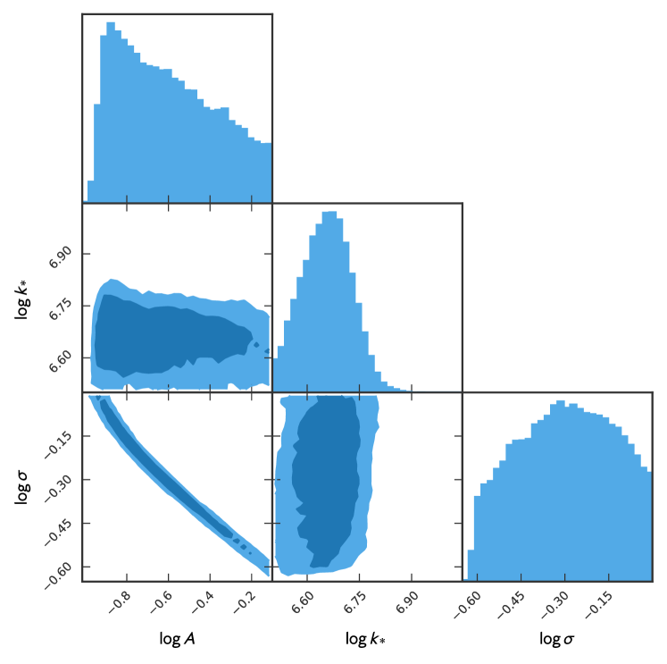
Figure 1: The posterior distribution of the Bayesian parameter estimation. The contours in the 2D distribution represent $1\sigma$ and $2\sigma$ regions respectively.

We report our analysis in Fig. 1. The median value of the parameters and their $95\%$ equal-tailed credible intervals are $A=0.24^{+0.42}_{-0.11}$, $k_{*}=4.53^{+1.32}_{-1.06}\times 10^{6}\mathrm{Mpc}^{-1}$ and $\sigma=0.51^{+0.40}_{-0.24}$. Moreover, fraction of PBHs in DM is evaluated to be $f_{\mathrm{PBH}}=3.54^{+7.66}_{-2.82}\times 10^{-3}$ and the local merger rate is given by $\mathcal{R}=3836^{+30906}_{-3670}\mathrm{Gpc}^{-3}\mathrm{yr}^{-1}$. The sensitivity volume values from the O3 run in the SSM search for SSM200308 is $\left\langle VT\right\rangle\simeq 3\times 10^{-4}\mathrm{Gpc}^{3}\mathrm{yr}$ Abbott et al. (2023b). Therefore, the expected event numbers are $N=\mathcal{R}\left\langle VT\right\rangle=1.05^{+8.50}_{-1.01}$ which is consistent with Phukon et al. (2021); Abbott et al. (2023b).

Furthermore, we demonstrate the PBH mass function in Fig. 2, together with the median mass of SSM200803. We also show the constraints on $f_{\mathrm{PBH}}$ by EROS/MACHO microlensing Tisserand et al. (2007), OGLE microlensing Niikura et al. (2019), SGWB from binary PBHs Wang et al. (2018); Chen and Huang (2019), dynamical heating of ultra-faint dwarf galaxies (UFD) Brandt (2016) and accretion constraints of CMB Ali-Haimoud and Kamionkowski (2017); Aloni et al. (2017); Horowitz (2016); Chen et al. (2016); Poulin et al. (2017). It can be seen that the reconstructed mass function (or the abundance that $f_{\mathrm{PBH}}=3.54^{+7.66}_{-2.82}\times 10^{-3}$) is consistent with current observational constraints.

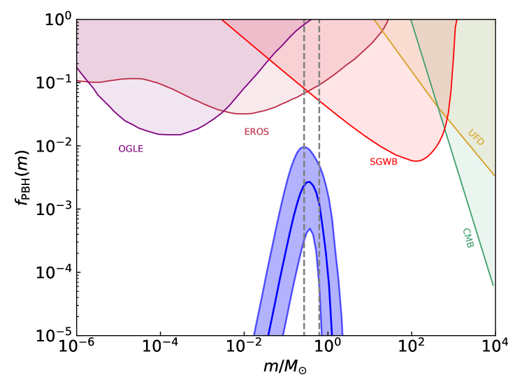
Figure 2: The posterior distribution of the PBH mass function. The blue bands represent the region at $95\%$ confidence level. The gray dashed lines are the median mass of SSM200803. We also present the current constraints on $f_{\mathrm{PBH}}$.

III SGWB associated with PBHs

The incoherent superposition of the GWs from all the emitting sources all over the sky will generate an SGWB. In this section, we will demonstrate the SIGWs associated with the formation of PBHs and the SGWB from the merger of binary PBHs if the SSM200308 can be explained by PBHs.

III.1 Scalar-Induced Gravitatiaonal Waves

The second-order tensor modes in the perturbed FRW metric will be sourced by the quadratic terms of linear curvature perturbations. These second-order GWs are inevitably generated during the formation of PBHs and their unique scaling in the low-frequency region provides a smoking gun in hunting PBHs Yuan et al. (2019, 2023). The perturbed metric in Newtonian gauge in the absence of vector perturbations, linear tensor perturbations and anisotropies stress is given by

$$\mathrm{d}s^{2}=a^{2}\left\{-(1+2\phi)\mathrm{d}\eta^{2}+\left[(1-2\phi)\delta_{ij}+\frac{h_{ij}}{2}\right]\mathrm{d}x^{i}\mathrm{~{}d}x^{j}\right\},$$ (11)

where the Bardeen potential $\phi$ is related to the comoving curvature perturbations through $\phi=-2/3\zeta$. The equation of motion for the second-order tensor mode is given by

$$h_{ij}^{\prime\prime}+2\mathcal{H}h_{ij}^{\prime}-\nabla^{2}h_{ij}=-4\mathcal{T}_{ij}^{\ell m}\mathcal{S}_{\ell m},$$ (12)

where the projection operator $\mathcal{T}_{ij}^{\ell m}$ picks out the transverse and traceless part of the source term. During radiation dominant, the source term is given by

$$S_{ij}=2\phi\partial_{i}\partial_{j}\phi-\frac{4}{3(1+w)}\left(\partial_{i}\phi+\frac{\partial_{i}\phi^{\prime}}{\mathcal{H}(\eta)}\right)\left(\partial_{j}\phi+\frac{\partial_{j}\phi^{\prime}}{\mathcal{H}(\eta)}\right).$$ (13)

Following Kohri and Terada (2018), the solution to Eq. (12) can be solved by the Green’s function and the energy spectrum of SIGWs, $\Omega_{\mathrm{GW}}$, which is defined as the energy of GWs per logarithm wavelength normalized by the critical energy of the Universe, can be computed in a semi-analytical way such that Kohri and Terada (2018)

$$\Omega_{\mathrm{GW}}(f) =\frac{\Omega_{\mathrm{r}}}{6}\left(\frac{g_{*}}{g_{*}^{0}}\right)\left(\frac{g_{*s}}{g_{*s}^{0}}\right)^{-4/3}\int_{0}^{\infty}\mathrm{d}u\int_{|1-u|}^{1+u}\mathrm{~{}d}v$$ (14)

$$\frac{v^{2}}{u^{2}}\left[1-\left(\frac{1+v^{2}-u^{2}}{2v}\right)^{2}\right]^{2}\mathcal{P}_{\zeta}(uk)\mathcal{P}_{\zeta}(vk)\overline{I^{2}(u,v)},$$

where $k=2\pi f$ and $\Omega_{r}=9\times 10^{-5}$ is the density parameter for radiation. $g_{*}$ and $g_{*s}$ stand for the effective degrees of freedom of entropy and energy respectively. The kernel function $\overline{I^{2}(u,v)}$ is given by Kohri and Terada (2018):

$$\overline{I^{2}(u,v)}=\frac{9(u^{2}+v^{2}-3)^{2}}{32u^{6}v^{6}}\Bigg{\{}\Big{(}-4uv+(u^{2}+v^{2}-3)$$ (15)

$$\times\ln\Big{|}{3-(u+v)^{2}\over 3-(u-v)^{2}}\Big{|}\Big{)}^{2}+\pi^{2}\left(u^{2}+v^{2}-3\right)^{2}\Theta(u+v-\sqrt{3})\Bigg{\}}.$$

III.2 SGWB form binary PBH coalescences

The SGWB generated by binary PBH coalescences all over the sky can be evaluated as Phinney (2001); Regimbau and Mandic (2008); Zhu et al. (2011, 2013)

$$\Omega_{\mathrm{GW}}(f)=\frac{f}{\rho_{c}}\int dM_{1}dM_{2}dz\frac{dt}{dz}R(z,M_{1},M_{2})\frac{dE_{s}}{df_{s}},$$ (16)

with $dt/dz$ being the derivative of the lookback time to the redshift, which takes the form

$$\frac{dt}{dz}=\frac{1}{H_{0}\sqrt{\Delta}(1+z)}.$$ (17)

Here $H_{0}$ is the Hubble value by today, $\Delta=\Omega_{r}(1+z)^{4}+\Omega_{m}(1+z)^{3}+\Omega_{\Lambda}$, $\Omega_{m}$ and $\Omega_{\Lambda}$ are density parameters for matter and dark energy respectively Aghanim et al. (2020). The energy spectrum of a single PBH coalescence event in the source frame, ${dE_{s}}/{df_{s}}$, can be found in Cutler et al. (1993); Chernoff and Finn (1993); Zhu et al. (2011).

The median value and the $95\%$ intervals of SIGWs and SGWB from binary PBH coalescences are illustrated in Fig. 3 using the posterior of $A$, $K_{*}$ and $\sigma$ obtained in Section. II together with the power-law integrated sensitivity curves of LIGO O3, LIGO at design sensitivity Thrane and Romano (2013), Cosmic Explorer (CE) Abbott et al. (2017), Einstein Telescope (ET) Punturo et al. (2010) and the constraints from NANOGrav 15yr dataset Afzal et al. (2023).

It can be seen that the SGWB form binary PBHs is below the sensitivity of LIGO O3 but it could be verified by CE and ET in the future. However, the resulting SIGWs exceed the upper limits of NANOGrav 15yr, indicating a discrepancy for PBHs generated by the collapse of Gaussian perturbations to explain SSM200803.

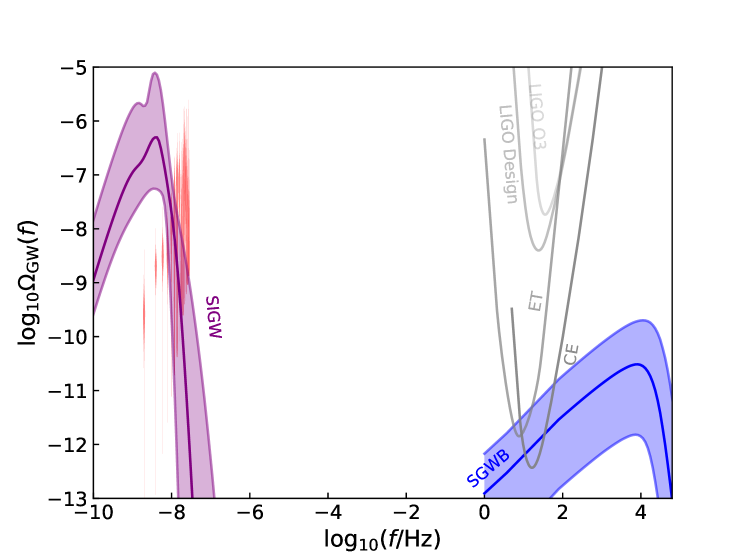
Figure 3: The SIGW (purple lines) and SGWB from binary PBHs (blue lines) if SSM200803 can be explained by PBHs. The violin polot represents the NANOGrav 15yr dataset Agazie et al. (2023). The purple and blue bands represent the the region at $95\%$ confidence level for SIGWs and SGWB from binary PBHs respectively.

IV Conclusion and Discussion

In this study, we have delved into the potential explanation of SSM200308 as a consequence of PBHs emerging from the collapse of Gaussian perturbations in the early universe. Through a comprehensive Bayesian parameter estimation, we obtain the corresponding primordial curvature power spectrum that generates the PBHs for explaining SSM200308. Our findings indicate that although the merger rates of PBHs could be reconciled with the data and the SGWB from binary PBHs is consistent with current observations as long as PBHs constitute a few thousandths of the DM, the accompanied SIGWs during the formation of PBHs present a significant challenge. The SIGWs generated by the primordial curvature power spectrum would exceed the limits set by PTA observations, suggesting a discrepancy that questions the overdensities collapse as the origin of PBHs responsible for SSM200308.

However, SIGWs are related to PBHs formed by the collapse of overdensities. Given that the merger rate of PBHs is not sensitive with $P(m)$ and it is mainly dependent on $f_{\mathrm{PBH}}$. Therefore, the SGWB from binary PBH mergers would also be consistent with existing observations if the PBHs have other formation mechanisms, such as first-order phase transition Bagui et al. (2023). As a result, the SIGWs would disappear if PBHs had other formation mechanisms. In that case, our results cannot entirely rule out the possibility of PBHs in explaining SSM200803.

It’s worth mentioning that if primordial non-Gaussian effects are present during the formation of PBHs, the amplitude of the SIGWs could be suppressed Nakama et al. (2017); Garcia-Bellido et al. (2017); Unal (2019); Cai et al. (2019a, b); Yuan and Huang (2020); Ragavendra et al. (2020); Adshead et al. (2021); Abe et al. (2023); Yuan et al. (2023); Li et al. (2023, 2024); Perna et al. (2024), potentially explaining the results from NANOGrav Liu et al. (2024); Franciolini et al. (2023). Moreover, in this work, we focused on using the data from SSM200803. An even more intriguing result would be to use both results from NANOGrav 15yr and SSM200803 to place constraints on PBHs and the primordial non-Gaussianities. We leave this part for future work.

Acknowledgments. We thank Prunier et al. for sharing the data on the posterior distribution of SSM200803 Prunier et al. (2023). C.Y. thanks Antonio Riotto, Zu-cheng Chen, Yu-mei Wu and Shi Pi for useful discussions and valuable advice. This work is supported by the National Key Research and Development Program of China Grant No.2020YFC2201502, grants from NSFC (grant No. 11991052, 12047503), Key Research Program of Frontier Sciences, CAS, Grant NO. ZDBS-LY-7009. C.Y. acknowledges the financial support provided under the European Union’s H2020 ERC Advanced Grant “Black holes: gravitational engines of discovery” grant agreement no. Gravitas–101052587. Views and opinions expressed are however those of the author only and do not necessarily reflect those of the European Union or the European Research Council. Neither the European Union nor the granting authority can be held responsible for them. This project has received funding from the European Union’s Horizon 2020 research and innovation programme under the Marie Sklodowska-Curie grant agreement No 101007855. No 101007855.

References

- Abbott et al. (2016a) B. P. Abbott et al. (LIGO Scientific, Virgo), “Observation of Gravitational Waves from a Binary Black Hole Merger,” Phys. Rev. Lett. 116, 061102 (2016a), arXiv:1602.03837 [gr-qc] .
- Abbott et al. (2016b) B. P. Abbott et al. (LIGO Scientific, Virgo), “Binary Black Hole Mergers in the first Advanced LIGO Observing Run,” Phys. Rev. X 6, 041015 (2016b), [Erratum: Phys.Rev.X 8, 039903 (2018)], arXiv:1606.04856 [gr-qc] .
- Abbott et al. (2018a) B. P. Abbott et al. (LIGO Scientific, Virgo), “GWTC-1: A Gravitational-Wave Transient Catalog of Compact Binary Mergers Observed by LIGO and Virgo during the First and Second Observing Runs,” (2018a), arXiv:1811.12907 [astro-ph.HE] .
- Abbott et al. (2021) R. Abbott et al. (LIGO Scientific, Virgo), “GWTC-2: Compact Binary Coalescences Observed by LIGO and Virgo During the First Half of the Third Observing Run,” Phys. Rev. X 11, 021053 (2021), arXiv:2010.14527 [gr-qc] .
- Abbott et al. (2024) R. Abbott et al. (LIGO Scientific, VIRGO), “GWTC-2.1: Deep extended catalog of compact binary coalescences observed by LIGO and Virgo during the first half of the third observing run,” Phys. Rev. D 109, 022001 (2024), arXiv:2108.01045 [gr-qc] .
- Abbott et al. (2023a) R. Abbott et al. (KAGRA, VIRGO, LIGO Scientific), “GWTC-3: Compact Binary Coalescences Observed by LIGO and Virgo during the Second Part of the Third Observing Run,” Phys. Rev. X 13, 041039 (2023a), arXiv:2111.03606 [gr-qc] .
- Abbott et al. (2018b) B. P. Abbott et al. (LIGO Scientific, Virgo), “Search for Subsolar-Mass Ultracompact Binaries in Advanced LIGO’s First Observing Run,” Phys. Rev. Lett. 121, 231103 (2018b), arXiv:1808.04771 [astro-ph.CO] .
- Abbott et al. (2019) B. P. Abbott et al. (LIGO Scientific, Virgo), “Search for Subsolar Mass Ultracompact Binaries in Advanced LIGO’s Second Observing Run,” Phys. Rev. Lett. 123, 161102 (2019), arXiv:1904.08976 [astro-ph.CO] .
- Nitz and Wang (2021) Alexander H. Nitz and Yi-Fan Wang, “Search for gravitational waves from the coalescence of sub-solar mass and eccentric compact binaries,” (2021), 10.3847/1538-4357/ac01d9, arXiv:2102.00868 [astro-ph.HE] .
- Abbott et al. (2022) R. Abbott et al. (LIGO Scientific, VIRGO, KAGRA), “Search for Subsolar-Mass Binaries in the First Half of Advanced LIGO’s and Advanced Virgo’s Third Observing Run,” Phys. Rev. Lett. 129, 061104 (2022), arXiv:2109.12197 [astro-ph.CO] .
- Abbott et al. (2023b) R. Abbott et al. (LIGO Scientific, VIRGO, KAGRA), “Search for subsolar-mass black hole binaries in the second part of Advanced LIGO’s and Advanced Virgo’s third observing run,” Mon. Not. Roy. Astron. Soc. 524, 5984–5992 (2023b), [Erratum: Mon.Not.Roy.Astron.Soc. 526, 6234 (2023)], arXiv:2212.01477 [astro-ph.HE] .
- Nitz and Wang (2022) Alexander H. Nitz and Yi-Fan Wang, “Broad search for gravitational waves from subsolar-mass binaries through LIGO and Virgo’s third observing run,” Phys. Rev. D 106, 023024 (2022), arXiv:2202.11024 [astro-ph.HE] .
- Morras et al. (2023) Gonzalo Morras et al., “Analysis of a subsolar-mass compact binary candidate from the second observing run of Advanced LIGO,” Phys. Dark Univ. 42, 101285 (2023), arXiv:2301.11619 [gr-qc] .
- Prunier et al. (2023) Marine Prunier, Gonzalo Morrás, José Francisco Nuño Siles, Sebastien Clesse, Juan García-Bellido, and Ester Ruiz Morales, “Analysis of the subsolar-mass black hole candidate SSM200308 from the second part of the third observing run of Advanced LIGO-Virgo,” (2023), arXiv:2311.16085 [gr-qc] .
- Yamamoto et al. (2023) Takahiro S. Yamamoto, Ryoto Inui, Yuichiro Tada, and Shuichiro Yokoyama, “Prospects of detection of subsolar mass primordial black hole and white dwarf binary mergers,” (2023), arXiv:2401.00044 [gr-qc] .
- Carr et al. (2024) Bernard Carr, Sebastien Clesse, Juan Garcia-Bellido, Michael Hawkins, and Florian Kuhnel, “Observational evidence for primordial black holes: A positivist perspective,” Phys. Rept. 1054, 1–68 (2024), arXiv:2306.03903 [astro-ph.CO] .
- Crescimbeni et al. (2024) F. Crescimbeni, G. Franciolini, P. Pani, and A. Riotto, “Primordial black holes or else? Tidal tests on subsolar mass gravitational-wave observations,” (2024), arXiv:2402.18656 [astro-ph.HE] .
- Zel’dovich and Novikov (1967) Ya. B. Zel’dovich and I. D. Novikov, “The Hypothesis of Cores Retarded during Expansion and the Hot Cosmological Model,” Sov. Astron. 10, 602 (1967).
- Hawking (1971) Stephen Hawking, “Gravitationally collapsed objects of very low mass,” Mon. Not. Roy. Astron. Soc. 152, 75 (1971).
- Carr and Hawking (1974) Bernard J. Carr and S. W. Hawking, “Black holes in the early Universe,” Mon. Not. Roy. Astron. Soc. 168, 399–415 (1974).
- Carr (1975) Bernard J. Carr, “The Primordial black hole mass spectrum,” Astrophys. J. 201, 1–19 (1975).
- Cai et al. (2018) Yi-Fu Cai, Xi Tong, Dong-Gang Wang, and Sheng-Feng Yan, “Primordial Black Holes from Sound Speed Resonance during Inflation,” Phys. Rev. Lett. 121, 081306 (2018), arXiv:1805.03639 [astro-ph.CO] .
- Cotner and Kusenko (2017) Eric Cotner and Alexander Kusenko, “Primordial black holes from supersymmetry in the early universe,” Phys. Rev. Lett. 119, 031103 (2017), arXiv:1612.02529 [astro-ph.CO] .
- Espinosa et al. (2018) J. R. Espinosa, D. Racco, and A. Riotto, “Cosmological Signature of the Standard Model Higgs Vacuum Instability: Primordial Black Holes as Dark Matter,” Phys. Rev. Lett. 120, 121301 (2018), arXiv:1710.11196 [hep-ph] .
- Palma et al. (2020) Gonzalo A. Palma, Spyros Sypsas, and Cristobal Zenteno, “Seeding primordial black holes in multifield inflation,” Phys. Rev. Lett. 125, 121301 (2020), arXiv:2004.06106 [astro-ph.CO] .
- Pi and Sasaki (2023) Shi Pi and Misao Sasaki, “Primordial black hole formation in nonminimal curvaton scenarios,” Phys. Rev. D 108, L101301 (2023), arXiv:2112.12680 [astro-ph.CO] .
- Meng et al. (2023) De-Shuang Meng, Chen Yuan, and Qing-Guo Huang, “Primordial black holes generated by the non-minimal spectator field,” Sci. China Phys. Mech. Astron. 66, 280411 (2023), arXiv:2212.03577 [astro-ph.CO] .
- Aghanim et al. (2020) N. Aghanim et al. (Planck), “Planck 2018 results. VI. Cosmological parameters,” Astron. Astrophys. 641, A6 (2020), [Erratum: Astron.Astrophys. 652, C4 (2021)], arXiv:1807.06209 [astro-ph.CO] .
- Sasaki et al. (2016) Misao Sasaki, Teruaki Suyama, Takahiro Tanaka, and Shuichiro Yokoyama, “Primordial Black Hole Scenario for the Gravitational-Wave Event GW150914,” Phys. Rev. Lett. 117, 061101 (2016), [erratum: Phys. Rev. Lett.121,no.5,059901(2018)], arXiv:1603.08338 [astro-ph.CO] .
- Chen and Huang (2018) Zu-Cheng Chen and Qing-Guo Huang, “Merger Rate Distribution of Primordial-Black-Hole Binaries,” Astrophys. J. 864, 61 (2018), arXiv:1801.10327 [astro-ph.CO] .
- Raidal et al. (2019) Martti Raidal, Christian Spethmann, Ville Vaskonen, and Hardi Veermäe, “Formation and Evolution of Primordial Black Hole Binaries in the Early Universe,” JCAP 1902, 018 (2019), arXiv:1812.01930 [astro-ph.CO] .
- De Luca et al. (2020) V. De Luca, G. Franciolini, P. Pani, and A. Riotto, “Primordial Black Holes Confront LIGO/Virgo data: Current situation,” JCAP 06, 044 (2020), arXiv:2005.05641 [astro-ph.CO] .
- Hall et al. (2020) Alex Hall, Andrew D. Gow, and Christian T. Byrnes, “Bayesian analysis of LIGO-Virgo mergers: Primordial vs. astrophysical black hole populations,” Phys. Rev. D 102, 123524 (2020), arXiv:2008.13704 [astro-ph.CO] .
- Bhagwat et al. (2021) S. Bhagwat, V. De Luca, G. Franciolini, P. Pani, and A. Riotto, “The importance of priors on LIGO-Virgo parameter estimation: the case of primordial black holes,” JCAP 01, 037 (2021), arXiv:2008.12320 [astro-ph.CO] .
- Hütsi et al. (2020) Gert Hütsi, Martti Raidal, Ville Vaskonen, and Hardi Veermäe, “Two populations of LIGO-Virgo black holes,” (2020), arXiv:2012.02786 [astro-ph.CO] .
- Wong et al. (2021) Kaze W. K. Wong, Gabriele Franciolini, Valerio De Luca, Vishal Baibhav, Emanuele Berti, Paolo Pani, and Antonio Riotto, “Constraining the primordial black hole scenario with Bayesian inference and machine learning: the GWTC-2 gravitational wave catalog,” Phys. Rev. D 103, 023026 (2021), arXiv:2011.01865 [gr-qc] .
- De Luca et al. (2021) V. De Luca, G. Franciolini, P. Pani, and A. Riotto, “Bayesian Evidence for Both Astrophysical and Primordial Black Holes: Mapping the GWTC-2 Catalog to Third-Generation Detectors,” JCAP 05, 003 (2021), arXiv:2102.03809 [astro-ph.CO] .
- Bavera et al. (2022) Simone S. Bavera, Gabriele Franciolini, Giulia Cusin, Antonio Riotto, Michael Zevin, and Tassos Fragos, “Stochastic gravitational-wave background as a tool for investigating multi-channel astrophysical and primordial black-hole mergers,” Astron. Astrophys. 660, A26 (2022), arXiv:2109.05836 [astro-ph.CO] .
- Franciolini et al. (2021) Gabriele Franciolini, Vishal Baibhav, Valerio De Luca, Ken K. Y. Ng, Kaze W. K. Wong, Emanuele Berti, Paolo Pani, Antonio Riotto, and Salvatore Vitale, “Quantifying the evidence for primordial black holes in LIGO/Virgo gravitational-wave data,” (2021), arXiv:2105.03349 [gr-qc] .
- Chen et al. (2022) Zu-Cheng Chen, Chen Yuan, and Qing-Guo Huang, “Confronting the primordial black hole scenario with the gravitational-wave events detected by LIGO-Virgo,” Phys. Lett. B 829, 137040 (2022), arXiv:2108.11740 [astro-ph.CO] .
- Chen and Hall (2024) Zu-Cheng Chen and Alex Hall, “Confronting primordial black holes with LIGO-Virgo-KAGRA and the Einstein Telescope,” (2024), arXiv:2402.03934 [astro-ph.CO] .
- Tomita (1967) Kenji Tomita, “Non-linear theory of gravitational instability in the expanding universe,” Progress of Theoretical Physics 37, 831–846 (1967).
- Matarrese et al. (1993) Sabino Matarrese, Ornella Pantano, and Diego Saez, “A General relativistic approach to the nonlinear evolution of collisionless matter,” Phys. Rev. D47, 1311–1323 (1993).
- Matarrese et al. (1994) Sabino Matarrese, Ornella Pantano, and Diego Saez, “General relativistic dynamics of irrotational dust: Cosmological implications,” Phys. Rev. Lett. 72, 320–323 (1994), arXiv:astro-ph/9310036 [astro-ph] .
- Ananda et al. (2007) Kishore N. Ananda, Chris Clarkson, and David Wands, “The Cosmological gravitational wave background from primordial density perturbations,” Phys. Rev. D75, 123518 (2007), arXiv:gr-qc/0612013 [gr-qc] .
- Baumann et al. (2007) Daniel Baumann, Paul J. Steinhardt, Keitaro Takahashi, and Kiyotomo Ichiki, “Gravitational Wave Spectrum Induced by Primordial Scalar Perturbations,” Phys. Rev. D76, 084019 (2007), arXiv:hep-th/0703290 [hep-th] .
- Saito and Yokoyama (2009) Ryo Saito and Jun’ichi Yokoyama, “Gravitational wave background as a probe of the primordial black hole abundance,” Phys. Rev. Lett. 102, 161101 (2009), [Erratum: Phys. Rev. Lett.107,069901(2011)], arXiv:0812.4339 [astro-ph] .
- Saito and Yokoyama (2010) Ryo Saito and Jun’ichi Yokoyama, “Gravitational-Wave Constraints on the Abundance of Primordial Black Holes,” Prog. Theor. Phys. 123, 867–886 (2010), [Erratum: Prog. Theor. Phys.126,351(2011)], arXiv:0912.5317 [astro-ph.CO] .
- Yuan et al. (2019) Chen Yuan, Zu-Cheng Chen, and Qing-Guo Huang, “Log-dependent slope of scalar induced gravitational waves in the infrared regions,” (2019), arXiv:1910.09099 [astro-ph.CO] .
- Yuan et al. (2023) Chen Yuan, De-Shuang Meng, and Qing-Guo Huang, “Full analysis of the scalar-induced gravitational waves for the curvature perturbation with local-type non-Gaussianities,” JCAP 12, 036 (2023), arXiv:2308.07155 [astro-ph.CO] .
- Yuan and Huang (2021) Chen Yuan and Qing-Guo Huang, “A topic review on probing primordial black hole dark matter with scalar induced gravitational waves,” (2021), arXiv:2103.04739 [astro-ph.GA] .
- Domènech (2021) Guillem Domènech, “Scalar Induced Gravitational Waves Review,” Universe 7, 398 (2021), arXiv:2109.01398 [gr-qc] .
- Abbott et al. (2016c) B. P. Abbott et al. (LIGO Scientific, Virgo), “The Rate of Binary Black Hole Mergers Inferred from Advanced LIGO Observations Surrounding GW150914,” Astrophys. J. Lett. 833, L1 (2016c), arXiv:1602.03842 [astro-ph.HE] .
- Abbott et al. (2016d) B. P. Abbott et al. (LIGO Scientific, Virgo), “Supplement: The Rate of Binary Black Hole Mergers Inferred from Advanced LIGO Observations Surrounding GW150914,” Astrophys. J. Suppl. 227, 14 (2016d), arXiv:1606.03939 [astro-ph.HE] .
- Abbott et al. (2016e) B. P. Abbott et al. (LIGO Scientific, Virgo), “Binary Black Hole Mergers in the first Advanced LIGO Observing Run,” Phys. Rev. X6, 041015 (2016e), [erratum: Phys. Rev.X8,no.3,039903(2018)], arXiv:1606.04856 [gr-qc] .
- Wysocki et al. (2019) Daniel Wysocki, Jacob Lange, and Richard O’Shaughnessy, “Reconstructing phenomenological distributions of compact binaries via gravitational wave observations,” Phys. Rev. D 100, 043012 (2019), arXiv:1805.06442 [gr-qc] .
- Fishbach et al. (2018) Maya Fishbach, Daniel E. Holz, and Will M. Farr, “Does the Black Hole Merger Rate Evolve with Redshift?” Astrophys. J. Lett. 863, L41 (2018), arXiv:1805.10270 [astro-ph.HE] .
- Mandel et al. (2019) Ilya Mandel, Will M. Farr, and Jonathan R. Gair, “Extracting distribution parameters from multiple uncertain observations with selection biases,” Mon. Not. Roy. Astron. Soc. 486, 1086–1093 (2019), arXiv:1809.02063 [physics.data-an] .
- Thrane and Talbot (2019) Eric Thrane and Colm Talbot, “An introduction to Bayesian inference in gravitational-wave astronomy: parameter estimation, model selection, and hierarchical models,” Publ. Astron. Soc. Austral. 36, e010 (2019), [Erratum: Publ.Astron.Soc.Austral. 37, e036 (2020)], arXiv:1809.02293 [astro-ph.IM] .
- Ali-Haïmoud et al. (2017) Yacine Ali-Haïmoud, Ely D. Kovetz, and Marc Kamionkowski, “Merger rate of primordial black-hole binaries,” Phys. Rev. D96, 123523 (2017), arXiv:1709.06576 [astro-ph.CO] .
- Harada et al. (2015) Tomohiro Harada, Chul-Moon Yoo, Tomohiro Nakama, and Yasutaka Koga, “Cosmological long-wavelength solutions and primordial black hole formation,” Phys. Rev. D 91, 084057 (2015), arXiv:1503.03934 [gr-qc] .
- Musco and Miller (2013) Ilia Musco and John C. Miller, “Primordial black hole formation in the early universe: critical behaviour and self-similarity,” Class. Quant. Grav. 30, 145009 (2013), arXiv:1201.2379 [gr-qc] .
- Saikawa and Shirai (2018) Ken’ichi Saikawa and Satoshi Shirai, “Primordial gravitational waves, precisely: The role of thermodynamics in the Standard Model,” JCAP 05, 035 (2018), arXiv:1803.01038 [hep-ph] .
- Borsanyi et al. (2016) Sz. Borsanyi et al., “Calculation of the axion mass based on high-temperature lattice quantum chromodynamics,” Nature 539, 69–71 (2016), arXiv:1606.07494 [hep-lat] .
- Franciolini et al. (2022) Gabriele Franciolini, Ilia Musco, Paolo Pani, and Alfredo Urbano, “From inflation to black hole mergers and back again: Gravitational-wave data-driven constraints on inflationary scenarios with a first-principle model of primordial black holes across the QCD epoch,” Phys. Rev. D 106, 123526 (2022), arXiv:2209.05959 [astro-ph.CO] .
- Musco et al. (2023) Ilia Musco, Karsten Jedamzik, and Sam Young, “Primordial black hole formation during the QCD phase transition: threshold, mass distribution and abundance,” (2023), arXiv:2303.07980 [astro-ph.CO] .
- Choptuik (1993) Matthew W. Choptuik, “Universality and scaling in gravitational collapse of a massless scalar field,” Phys. Rev. Lett. 70, 9–12 (1993).
- Evans and Coleman (1994) Charles R. Evans and Jason S. Coleman, “Observation of critical phenomena and selfsimilarity in the gravitational collapse of radiation fluid,” Phys. Rev. Lett. 72, 1782–1785 (1994), arXiv:gr-qc/9402041 .
- Niemeyer and Jedamzik (1998) Jens C. Niemeyer and K. Jedamzik, “Near-critical gravitational collapse and the initial mass function of primordial black holes,” Phys. Rev. Lett. 80, 5481–5484 (1998), arXiv:astro-ph/9709072 .
- Koike et al. (1995) Tatsuhiko Koike, Takashi Hara, and Satoshi Adachi, “Critical behavior in gravitational collapse of radiation fluid: A Renormalization group (linear perturbation) analysis,” Phys. Rev. Lett. 74, 5170–5173 (1995), arXiv:gr-qc/9503007 .
- Ferrante et al. (2023) Giacomo Ferrante, Gabriele Franciolini, Antonio Iovino, Junior., and Alfredo Urbano, “Primordial non-Gaussianity up to all orders: Theoretical aspects and implications for primordial black hole models,” Phys. Rev. D 107, 043520 (2023), arXiv:2211.01728 [astro-ph.CO] .
- Gow et al. (2023) Andrew D. Gow, Hooshyar Assadullahi, Joseph H. P. Jackson, Kazuya Koyama, Vincent Vennin, and David Wands, “Non-perturbative non-Gaussianity and primordial black holes,” EPL 142, 49001 (2023), arXiv:2211.08348 [astro-ph.CO] .
- Ianniccari et al. (2024) A. Ianniccari, A. J. Iovino, A. Kehagias, D. Perrone, and A. Riotto, “The Primordial Black Hole Abundance: The Broader, the Better,” (2024), arXiv:2402.11033 [astro-ph.CO] .
- Pi and Sasaki (2020) Shi Pi and Misao Sasaki, “Gravitational Waves Induced by Scalar Perturbations with a Lognormal Peak,” JCAP 09, 037 (2020), arXiv:2005.12306 [gr-qc] .
- Domènech et al. (2020) Guillem Domènech, Shi Pi, and Misao Sasaki, “Induced gravitational waves as a probe of thermal history of the universe,” JCAP 08, 017 (2020), arXiv:2005.12314 [gr-qc] .
- Yuan and Huang (2020) Chen Yuan and Qing-Guo Huang, “Gravitational waves induced by the local-type non-Gaussian curvature perturbations,” (2020), arXiv:2007.10686 [astro-ph.CO] .
- Meng et al. (2022) De-Shuang Meng, Chen Yuan, and Qing-guo Huang, “One-loop correction to the enhanced curvature perturbation with local-type non-Gaussianity for the formation of primordial black holes,” Phys. Rev. D 106, 063508 (2022), arXiv:2207.07668 [astro-ph.CO] .
- Gorji and Sasaki (2023) Mohammad Ali Gorji and Misao Sasaki, “Primordial-tensor-induced stochastic gravitational waves,” Phys. Lett. B 846, 138236 (2023), arXiv:2302.14080 [gr-qc] .
- Franciolini et al. (2023) Gabriele Franciolini, Antonio Iovino, Junior., Ville Vaskonen, and Hardi Veermae, “Recent Gravitational Wave Observation by Pulsar Timing Arrays and Primordial Black Holes: The Importance of Non-Gaussianities,” Phys. Rev. Lett. 131, 201401 (2023), arXiv:2306.17149 [astro-ph.CO] .
- Papanikolaou et al. (2024) Theodoros Papanikolaou, Xin-Chen He, Xiao-Han Ma, Yi-Fu Cai, Emmanuel N. Saridakis, and Misao Sasaki, “New probe of non-Gaussianities with primordial black hole induced gravitational waves,” (2024), arXiv:2403.00660 [astro-ph.CO] .
- Ando et al. (2018) Kenta Ando, Keisuke Inomata, and Masahiro Kawasaki, “Primordial black holes and uncertainties in the choice of the window function,” Phys. Rev. D 97, 103528 (2018), arXiv:1802.06393 [astro-ph.CO] .
- Young (2019) Sam Young, “The primordial black hole formation criterion re-examined: Parametrisation, timing and the choice of window function,” Int. J. Mod. Phys. D 29, 2030002 (2019), arXiv:1905.01230 [astro-ph.CO] .
- Phukon et al. (2021) Khun Sang Phukon, Gregory Baltus, Sarah Caudill, Sebastien Clesse, Antoine Depasse, Maxime Fays, Heather Fong, Shasvath J. Kapadia, Ryan Magee, and Andres Jorge Tanasijczuk, “The hunt for sub-solar primordial black holes in low mass ratio binaries is open,” (2021), arXiv:2105.11449 [astro-ph.CO] .
- Tisserand et al. (2007) P. Tisserand et al. (EROS-2), “Limits on the Macho Content of the Galactic Halo from the EROS-2 Survey of the Magellanic Clouds,” Astron. Astrophys. 469, 387–404 (2007), arXiv:astro-ph/0607207 .
- Niikura et al. (2019) Hiroko Niikura, Masahiro Takada, Shuichiro Yokoyama, Takahiro Sumi, and Shogo Masaki, “Constraints on Earth-mass primordial black holes from OGLE 5-year microlensing events,” Phys. Rev. D99, 083503 (2019), arXiv:1901.07120 [astro-ph.CO] .
- Wang et al. (2018) Sai Wang, Yi-Fan Wang, Qing-Guo Huang, and Tjonnie G. F. Li, “Constraints on the Primordial Black Hole Abundance from the First Advanced LIGO Observation Run Using the Stochastic Gravitational-Wave Background,” Phys. Rev. Lett. 120, 191102 (2018), arXiv:1610.08725 [astro-ph.CO] .
- Chen and Huang (2019) Zu-Cheng Chen and Qing-Guo Huang, “Distinguishing Primordial Black Holes from Astrophysical Black Holes by Einstein Telescope and Cosmic Explorer,” (2019), arXiv:1904.02396 [astro-ph.CO] .
- Brandt (2016) Timothy D. Brandt, “Constraints on MACHO Dark Matter from Compact Stellar Systems in Ultra-Faint Dwarf Galaxies,” Astrophys. J. 824, L31 (2016), arXiv:1605.03665 [astro-ph.GA] .
- Ali-Haimoud and Kamionkowski (2017) Yacine Ali-Haimoud and Marc Kamionkowski, “Cosmic microwave background limits on accreting primordial black holes,” Phys. Rev. D95, 043534 (2017), arXiv:1612.05644 [astro-ph.CO] .
- Aloni et al. (2017) Daniel Aloni, Kfir Blum, and Raphael Flauger, “Cosmic microwave background constraints on primordial black hole dark matter,” JCAP 1705, 017 (2017), arXiv:1612.06811 [astro-ph.CO] .
- Horowitz (2016) Benjamin Horowitz, “Revisiting Primordial Black Holes Constraints from Ionization History,” (2016), arXiv:1612.07264 [astro-ph.CO] .
- Chen et al. (2016) Lu Chen, Qing-Guo Huang, and Ke Wang, “Constraint on the abundance of primordial black holes in dark matter from Planck data,” JCAP 1612, 044 (2016), arXiv:1608.02174 [astro-ph.CO] .
- Poulin et al. (2017) Vivian Poulin, Pasquale D. Serpico, Francesca Calore, Sebastien Clesse, and Kazunori Kohri, “CMB bounds on disk-accreting massive primordial black holes,” Phys. Rev. D96, 083524 (2017), arXiv:1707.04206 [astro-ph.CO] .
- Kohri and Terada (2018) Kazunori Kohri and Takahiro Terada, “Semianalytic calculation of gravitational wave spectrum nonlinearly induced from primordial curvature perturbations,” Phys. Rev. D97, 123532 (2018), arXiv:1804.08577 [gr-qc] .
- Phinney (2001) E. S. Phinney, “A Practical theorem on gravitational wave backgrounds,” astro-ph/0108028 (2001).
- Regimbau and Mandic (2008) T. Regimbau and V. Mandic, “Astrophysical Sources of Stochastic Gravitational-Wave Background,” Proceedings, 12th Workshop on Gravitational wave data analysis (GWDAW-12): Cambridge, USA, December 13-16, 2007, Class. Quant. Grav. 25, 184018 (2008), arXiv:0806.2794 [astro-ph] .
- Zhu et al. (2011) Xing-Jiang Zhu, E. Howell, T. Regimbau, D. Blair, and Zong-Hong Zhu, “Stochastic Gravitational Wave Background from Coalescing Binary Black Holes,” Astrophys. J. 739, 86 (2011), arXiv:1104.3565 [gr-qc] .
- Zhu et al. (2013) Xing-Jiang Zhu, Eric J. Howell, David G. Blair, and Zong-Hong Zhu, “On the gravitational wave background from compact binary coalescences in the band of ground-based interferometers,” Mon. Not. Roy. Astron. Soc. 431, 882–899 (2013), arXiv:1209.0595 [gr-qc] .
- Cutler et al. (1993) C. Cutler, Eric Poisson, G. J. Sussman, and L. S. Finn, “Gravitational radiation from a particle in circular orbit around a black hole. 2: Numerical results for the nonrotating case,” Phys. Rev. D47, 1511–1518 (1993).
- Chernoff and Finn (1993) David F. Chernoff and Lee Samuel Finn, “Gravitational radiation, inspiraling binaries, and cosmology,” Astrophys. J. 411, L5–L8 (1993), arXiv:gr-qc/9304020 [gr-qc] .
- Thrane and Romano (2013) Eric Thrane and Joseph D. Romano, “Sensitivity curves for searches for gravitational-wave backgrounds,” Phys. Rev. D88, 124032 (2013), arXiv:1310.5300 [astro-ph.IM] .
- Abbott et al. (2017) Benjamin P. Abbott et al. (LIGO Scientific), “Exploring the Sensitivity of Next Generation Gravitational Wave Detectors,” Class. Quant. Grav. 34, 044001 (2017), arXiv:1607.08697 [astro-ph.IM] .
- Punturo et al. (2010) M. Punturo et al., “The Einstein Telescope: A third-generation gravitational wave observatory,” Proceedings, 14th Workshop on Gravitational wave data analysis (GWDAW-14): Rome, Italy, January 26-29, 2010, Class. Quant. Grav. 27, 194002 (2010).
- Afzal et al. (2023) Adeela Afzal et al. (NANOGrav), “The NANOGrav 15 yr Data Set: Search for Signals from New Physics,” Astrophys. J. Lett. 951, L11 (2023), arXiv:2306.16219 [astro-ph.HE] .
- Agazie et al. (2023) Gabriella Agazie et al. (NANOGrav), “The NANOGrav 15 yr Data Set: Evidence for a Gravitational-wave Background,” Astrophys. J. Lett. 951, L8 (2023), arXiv:2306.16213 [astro-ph.HE] .
- Bagui et al. (2023) Eleni Bagui et al. (LISA Cosmology Working Group), “Primordial black holes and their gravitational-wave signatures,” (2023), arXiv:2310.19857 [astro-ph.CO] .
- Nakama et al. (2017) Tomohiro Nakama, Joseph Silk, and Marc Kamionkowski, “Stochastic gravitational waves associated with the formation of primordial black holes,” Phys. Rev. D95, 043511 (2017), arXiv:1612.06264 [astro-ph.CO] .
- Garcia-Bellido et al. (2017) Juan Garcia-Bellido, Marco Peloso, and Caner Unal, “Gravitational Wave signatures of inflationary models from Primordial Black Hole Dark Matter,” JCAP 09, 013 (2017), arXiv:1707.02441 [astro-ph.CO] .
- Unal (2019) Caner Unal, “Imprints of Primordial Non-Gaussianity on Gravitational Wave Spectrum,” Phys. Rev. D99, 041301 (2019), arXiv:1811.09151 [astro-ph.CO] .
- Cai et al. (2019a) Rong-gen Cai, Shi Pi, and Misao Sasaki, “Gravitational Waves Induced by non-Gaussian Scalar Perturbations,” Phys. Rev. Lett. 122, 201101 (2019a), arXiv:1810.11000 [astro-ph.CO] .
- Cai et al. (2019b) Rong-Gen Cai, Shi Pi, Shao-Jiang Wang, and Xing-Yu Yang, “Resonant multiple peaks in the induced gravitational waves,” JCAP 1905, 013 (2019b), arXiv:1901.10152 [astro-ph.CO] .
- Ragavendra et al. (2020) H. V. Ragavendra, Pankaj Saha, L. Sriramkumar, and Joseph Silk, “PBHs and secondary GWs from ultra slow roll and punctuated inflation,” (2020), arXiv:2008.12202 [astro-ph.CO] .
- Adshead et al. (2021) Peter Adshead, Kaloian D. Lozanov, and Zachary J. Weiner, “Non-Gaussianity and the induced gravitational wave background,” (2021), arXiv:2105.01659 [astro-ph.CO] .
- Abe et al. (2023) Katsuya T. Abe, Ryoto Inui, Yuichiro Tada, and Shuichiro Yokoyama, “Primordial black holes and gravitational waves induced by exponential-tailed perturbations,” JCAP 05, 044 (2023), arXiv:2209.13891 [astro-ph.CO] .
- Li et al. (2023) Jun-Peng Li, Sai Wang, Zhi-Chao Zhao, and Kazunori Kohri, “Complete Analysis of Scalar-Induced Gravitational Waves and Primordial Non-Gaussianities and ,” (2023), arXiv:2309.07792 [astro-ph.CO] .
- Li et al. (2024) Jun-Peng Li, Sai Wang, Zhi-Chao Zhao, and Kazunori Kohri, “Angular bispectrum and trispectrum of scalar-induced gravitational-waves: all contributions from primordial non-Gaussianity and ,” (2024), arXiv:2403.00238 [astro-ph.CO] .
- Perna et al. (2024) Gabriele Perna, Chiara Testini, Angelo Ricciardone, and Sabino Matarrese, “Fully non-Gaussian Scalar-Induced Gravitational Waves,” (2024), arXiv:2403.06962 [astro-ph.CO] .
- Liu et al. (2024) Lang Liu, Zu-Cheng Chen, and Qing-Guo Huang, “Implications for the non-Gaussianity of curvature perturbation from pulsar timing arrays,” Phys. Rev. D 109, L061301 (2024), arXiv:2307.01102 [astro-ph.CO] .