∎
The School of Cyber Security, University of Chinese Academy of Sciences, Beijing 100049, China.
sunshangquan@iie.ac.cn 33institutetext: Wenqi Ren 44institutetext: The School of Cyber Science and Technology, Shenzhen Campus of Sun Yat-sen University, Shenzhen 518107, China.
renwq3@mail.sysu.edu.cn 55institutetext: Jingyang Peng 66institutetext: Huawei Noah’s Ark Lab.
pengjingyang1@huawei.com 77institutetext: Fenglong Song 88institutetext: Huawei Noah’s Ark Lab.
songfenglong@huawei.com 99institutetext: Xiaochun Cao 1010institutetext: The School of Cyber Science and Technology, Shenzhen Campus of Sun Yat-sen University, Shenzhen 518107, China.
caoxiaochun@mail.sysu.edu.cn
DI-Retinex: Digital-Imaging Retinex Theory for Low-Light Image Enhancement
Abstract
Many existing methods for low-light image enhancement (LLIE) based on Retinex theory ignore important factors that affect the validity of this theory in digital imaging, such as noise, quantization error, non-linearity, and dynamic range overflow. In this paper, we propose a new expression called Digital-Imaging Retinex theory (DI-Retinex) through theoretical and experimental analysis of Retinex theory in digital imaging. Our new expression includes an offset term in the enhancement model, which allows for pixel-wise brightness contrast adjustment with a non-linear mapping function. In addition, to solve the low-light enhancement problem in an unsupervised manner, we propose an image-adaptive masked reverse degradation loss in Gamma space. We also design a variance suppression loss for regulating the additional offset term. Extensive experiments show that our proposed method outperforms all existing unsupervised methods in terms of visual quality, model size, and speed. Our algorithm can also assist downstream face detectors in low-light, as it shows the most performance gain after the low-light enhancement compared to other methods.
Keywords:
Low-light image enhancement Retinex theory face recognition1 Introduction
In low-light conditions, digital imaging often suffers from a number of degradations, such as low visibility and high levels of noise. While professional equipment and techniques such as long exposure, fill light, and large-aperture lenses can help alleviate these issues, many amateur photographers still struggle with low-light images. Therefore, there is a need for a portable and efficient low-light image enhancement (LLIE) algorithm that can effectively restore underexposed images.
Some fundamental works, e.g., Retinex theory (Land and McCann, 1971; Land, 1977), have attempted to explain the relation among scene radiance reaching human eyes, material reflectance, and source illumination. Many LLIE algorithms and models have been designed based on this theory. However, it is important to note that the original theory was developed for radiance reaching the retina, rather than for measuring imaging intensity in computer vision. Some LLIE works have recognized the issue of amplified noise after enhancement, but there are other important factors, such as quantization error, non-linearity, and dynamic range overflow, that have not been thoroughly discussed. Simply applying Retinex theory from optics to computer vision can lead to imprecision and incompleteness in LLIE.
In this study, we conduct a theoretical analysis of the various factors that can contribute to noise, quantization error, non-linearity, and dynamic range compression when applying Retinex theory to digital imaging. We propose an extended version of Retinex theory specifically designed for computer vision called Digital-Imaging Retinex theory (DI-Retinex). Through our analysis, we demonstrate the existence of an offset with a non-zero mean and an amplified variance that can be caused by these factors when applying DI-Retinex theory to low-light image enhancement.
Building on the observation and analysis of the DI-Retinex theory, we design a brightness contrast adjustment algorithm that addresses the LLIE problem using a lightweight network consisting of three convolutional layers. The network predicts the contrast and brightness coefficients in the brightness contrast adjustment function and enhances degraded images by plugging predictions in the function. To guide the network towards generating optimal coefficient pairs, we use a masked reverse degradation loss and a variance suppression loss, which enable the network to learn in a zero-shot manner111Zero-shot learning in low-level vision tasks represents the method requiring neither paired or unpaired training data, in contrast to its concept in high-level visual tasks (Li et al., 2021a; Zhang et al., 2019a)., without requiring paired or unpaired training data.
To sum up, our contributions can be summarized as:
-
•
We analyze Retinex theory from the perspective of optics and computational photography and discuss the variation when transferring it to digital imaging. In addition to noise, Retinex theory should also involve quantization error, non-linearity, and dynamic range overflow in its formulation. As such, we propose a new DI-Retinex theory specifically for LLIE.
-
•
We present a contrast brightness function to solve the LLIE problem derived from DI-Retinex theory. In addition, we propose a masked reverse degradation loss with Gamma encoding and a variance suppression loss to guide the network in a zero-shot learning manner.
-
•
Extensive experiments demonstrate that the proposed method outperforms all the zero-shot and unsupervised learning-based LLIE methods in terms of visual quality, objective metrics, model size and speed. Moreover, our approach can be used as a preprocessing step for downstream tasks such as detection.
2 Related Works
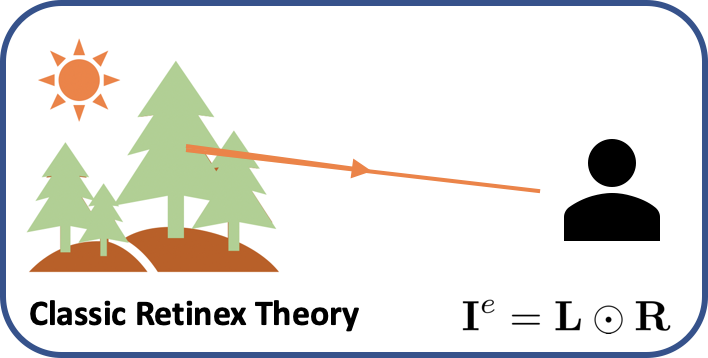
2.1 Classic Retinex Theory
Land and McCann (Land and McCann, 1971; Land, 1977) conducted a series of photometrical experiments, showing the scene radiance reaching human eye is the product of an intrinsic reflectance and incident illumination, which is named as Retinex Theory. It is formally written as follows,
| (1) |
where denotes Hadamard product, means radiance reaching human eye, is illuminance, and is reflectance. For images under different exposure conditions but with an identical scene, reflectance keeps unchanged since it is determined by and only related to the intrinsic material property of object surface. This also implies that sensation of color is mainly dependent on reflectance.
Many model-based methods employ Retinex theory for better modeling (Wang et al., 2013, 2014; Fu et al., 2014, 2016b; Guo et al., 2016; Fu et al., 2016a; Cai et al., 2017; Fu et al., 2018; Li et al., 2018b; Ren et al., 2018; Xu et al., 2020a). In recent years, deep learning with powerful learning ability and inference speed dominates the field of LLIE (Wei et al., 2018; Zhang et al., 2019b; Wang et al., 2019a, b; Fan et al., 2020; Yang et al., 2021b; Li et al., 2018a; Liu et al., 2021; Ma et al., 2022). Nearly one-third of deep learning methods also adopt Retinex theory for the sake of better enhancement effect and physical explanation (Li et al., 2021a). Therefore, a theoretical analysis of Retinex theory in digital photography is vital for establishing a valid physical model.
Note that the classic Retinex Theory has an assumption of proper exposure and the experiments of Land and McCann (Land and McCann, 1971; Land, 1977) with a telescopic photometer conclude that Eq. 1 holds for “eye” rather than camera. Simply borrowing Eq. 1 for solving LLIE problem may be inaccurate and incomplete due to violation of the assumption and condition.
Many existing methods (Jobson et al., 1997b, a; Ma et al., 2022; Wang et al., 2019a; Liu et al., 2021; Ying et al., 2017) presumably regard the reflectance component of Retinex theory as the final enhanced result, which is not what Retinex theory originally means and affects the final performance (Li et al., 2021a). Other methods (Li et al., 2018b; Zhang et al., 2019b; Ren et al., 2018) notice the existence of amplified noise. But they neglect other involved errors, e.g., quantization error and dynamic range compression, when transferring Retinex theory from optics to digital imaging.
2.2 Model-based LLIE Methods
The earlier LLIE methods use histogram equalization (HE) (Pizer, 1990; Abdullah-Al-Wadud et al., 2007) in global level (Coltuc et al., 2006; Ibrahim and Kong, 2007) and local region (Lee et al., 2013a; Stark, 2000). Other methods utilize Retinex-theory variants including classic Retinex theory (Fu et al., 2016b; Guo et al., 2016; Wang et al., 2014; Cai et al., 2017; Fu et al., 2016a; Xu et al., 2020a), single-scale Retinex (Jobson et al., 1997b), multi-scale Retinex (Jobson et al., 1997a), adaptive multi-scale Retinex (Lee et al., 2013b), Naturalness Retinex theory (Wang et al., 2013), Robust Retinex theory (Li et al., 2018b; Ren et al., 2018), for designing physically explicable algorithms where degraded image is decomposed into reflectance and illuminance during iterative optimization. There are also some methods (Dong et al., 2010; Li et al., 2015) transforming LLIE problem into a dehazing problem. The S-curve in photography can also be used to enhance underexposed image (Yuan and Sun, 2012).
2.3 Data-Drive LLIE Methods
Supervised Learning. With the developing of deep learning, the earliest deep learning-based LLIE methods focus on learning the mapping from low-light image to normal exposed one on paired training set. Various network architectures are developed for better enhancement, including a stacked-sparse denoising autoencoder in LLNet (Lore et al., 2017), U-Net (Chen et al., 2018), a multi-branch network named MBLLEN (Lv et al., 2018), Retinex-Net composed of a Decom-net and an Enhance-net (Wei et al., 2018), a lightweight LightenNet (Li et al., 2018a), a frequency decomposition network (Cai et al., 2018), a decoder network extracting global and local features (Wang et al., 2019a), siamese network (Chen et al., 2019), 3D U-Net (Jiang and Zheng, 2019; Zhang et al., 2021), progressive Retinex network (Wang et al., 2019b), three-branch subnetworks (Zhang et al., 2019b; Yang et al., 2021b), a complex Encoder-Decoder (Ren et al., 2019), a frequency-based decomposition-and-enhancement model (Xu et al., 2020b), a model integrating semantic segmentation (Fan et al., 2020), an edge-enhanced multi-exposure fusion network (Zhu et al., 2020b), residual network (Wang et al., 2020), a Retinex-inspired unrolling model by architecture search (Liu et al., 2021, 2022), Signal-to-Noise-Ratio (SNR)-aware transformer (Xu et al., 2022), a deep color consistent network (Zhang et al., 2022), a deep unfolding Retinex network (Wu et al., 2022), a normalizing flow model (Wang et al., 2022), Gamma correction model Wang et al. (2023a), contrastive self-distillation (Fu et al., 2023a), segmentation assisting model (Wu et al., 2023), structure-aware generator (Xu et al., 2023), vision Transformers (Cai et al., 2023) and diffusion models (Wang et al., 2023b; Yi et al., 2023). The above-mentioned architectures tend to be complicated and a large scale of paired training set with low/normal exposed images are necessary for training the networks. Large model size impedes fast inference speed. Besides, collecting large paired datasets are time-consuming and expansive in terms of human labours.
Semi-Supervised Learning. Several semi-supervised learning (SSL) methods (Yang et al., 2020, 2021a) use a deep recursive band network (DRBN) to learn a linear band representation between the pair of low-light image and corresponding ground-truth. For unpaired data, a perceptual quality-driven adversarial learning is adopted for guiding enhancement. The requirement of paired data still restricts the flexibility of the SSL methods.
Unpaired-supervised Learning. To alleviate the problem of lacking paired training data, unpaired supervised learning (UL) requires a set of normal exposed images unpaired with low-light images. EnlightenGAN (Jiang et al., 2021) employs adversarial learning with a local-global discriminator structure and a perceptual loss of self-regularization. NightEnhance (Jin et al., 2022) enhances night image with dark regions and light effects by a layer decomposition network and a light-effects suppression network with the guidance of multiple unsupervised layer-specific prior losses. However, in many common scenarios unpaired normally exposed images are still lacking or of low quality. The enhancement quality of UL methods highly relies on the quality of normally exposed images.
Zero-Shot Learning. To fully get rid of the limitation of paired data, zero-shot learning only needs low-light images for training. ExCNet (Zhang et al., 2019a) is composed of a neural network to estimate the S-curve to adjust luminance and map from back-lit input to enhanced output. The network is trained by minimizing a block-based energy expression as loss function. The idea of S-curve is adopted in Zero-DCE (Guo et al., 2020) and Zero-DCE++ (Li et al., 2021b) where a network estimating intermediate light-enhancement curve is used to restore input image iteratively. They design four sophisticated loss terms to regulate spatial consistency, exposure level, color constancy, and illumination smoothness. RRDNet (Zhu et al., 2020a) solves underexposed problem by decomposing reflectance, illumination and noise components by a three-branch network with three loss terms aiming at Retinex reconstruction, texture enhancement and illumination-guided noise estimation. RetinexDIP (Zhao et al., 2021) combines Deep Image Prior and Retinex decomposition and is guided by a group of component characteristics-related losses. SCI (Ma et al., 2022) incorporates a self-calibrated illumination module for the acceleration for training, a cooperative fidelity loss term and a smoothness loss term to achieve enhancement effect intrinsically. PairLIE (Fu et al., 2023b) leverages the pair of low-light images to train a self-learnining network based on Retinex theory. They are facing an unsatisfactory enhancement performance due to either delicate loss terms or the incompleteness of classic Retinex theory in LLIE task.
3 Analysis of Retinex Theory in Low-Light
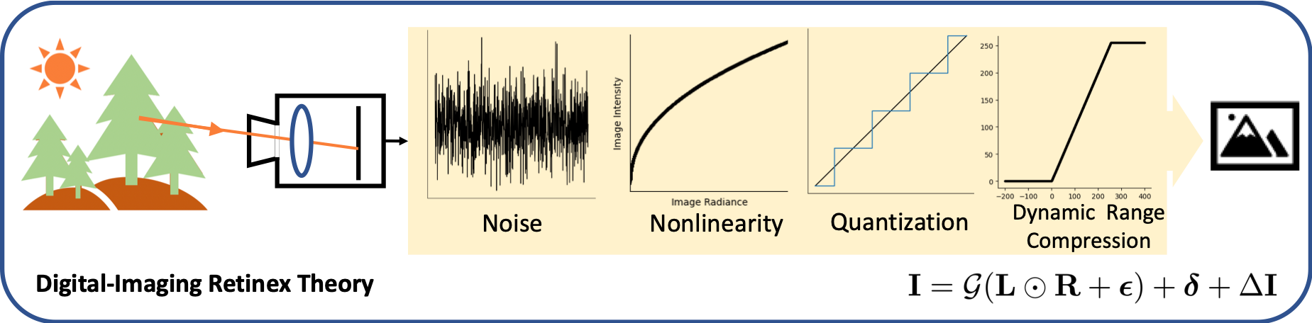
In this section, we first show the existence and cause of four factors influencing the expression of the classic Retinex theory, i.e., noise, quantization error, non-linearity mapping, and dynamic range overflow. Then a novel expression of DI-Retinex theory and its corresponding enhancement model are given based on the analysis.
3.1 Imaging Noise
When scene radiance reaches imaging devices, various sources of noise consisting of read noise (Janesick, 2007; Mackay et al., 2001), dark current noise (Moon et al., 2007; Healey and Kondepudy, 1994), photon shot noise (Schottky, 1918; Blanter and Büttiker, 2000), source follower noise (Antal et al., 2001) etc., are reported and should be taken into account (Haus, 2000). Therefore, Retinex theory is rewritten by taking noise into account, i.e.,
| (2) |
where is the combination of all significant noise sources during digital imaging. Among them, photon shot and dark current noise are theoretically modeled by Poisson distribution with parameters equal to ideal incoming photon and generated electrons respectively (Blanter and Büttiker, 2000; Moon et al., 2007). Though read noise, sometimes modeled by a Gaussian distribution, can be approximated by a Poisson distribution as well (Alter et al., 2006). In this work, we denote all noise sources as a whole by .
3.2 Non-linearity.
In a digital camera, an analog-to-digital converter (ADC) is deployed to convert voltage value with a range of to pixel intensity with a restricted range in RGB color space. A non-linear response function achieves the conversion, compensates the difference of human adaptation in dark and bright regions according to Weber’s Law (Weber, 1831), and suppresses representation space. The non-linear function can be commonly modeled by a Gamma transformation or Gamma encoding as follows (Mann and Picard, 1994; Mitsunaga and Nayar, 1999):
| (3) |
where is a coefficient set to nearly empirically, e.g., , and are two camera-specific parameters measuring bias and scale respectively.
3.3 Quantization error
Besides introducing non-linearity, the ADC converts a continuous voltage signal to a discrete -bit value. For example, in RGB () and RAW () color space, there are and possible pixel values for each channel, respectively. However, the conversion from continuous space to discrete one yields a quantization error that can be expressed by a uniform distribution:
| (4) |
where is the -th item of a quantization error , is the half of least significant bit . The discrete intensity can be formulated by continuous intensity plus a quantization noise, i.e., .
3.4 Dynamic Range Overflow
Another problem when transferring Retinex theory from human eyes to digital imaging is dynamic range limitation. Human eyes are known to have a significantly large dynamic range compared to vision sensors (Banterle et al., ). Therefore, scene dynamic range is presumably within the perceptual dynamic range of human eyes in the classic Retinex theory. However, a considerable scene dynamic range may exceed the physical tolerance of imaging devices. Therefore, a clamp function is defined as Eq. 5 to clip all exceeding values.
| (5) |
where is the max pixel value, e.g., in RGB space. By defining a masked offset matrix , clamp function can also be expressed as follows,
| (6) |
where has zero items at the pixels whose intensity and non-zero values with or with .
3.5 Digital-Imaging Retinex Theory
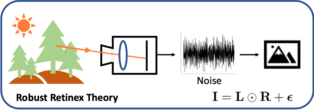
Combining all aforementioned factors, we reformulate the classic Retinex theory as follows:
| (7) |
The image irradiance perceived by the imaging device is ideal scene radiance plus a noise term. Then a camera response function is applied to the noisy irradiance. Finally, a quantization noise and a masked offset due to dynamic range compression are added. A comparison of the diagrams of our DI-Retinex theory and previous Retinex theories is shown in Fig. 2. Despite the complicated expression, it can be utilized to derive an efficient LLIE model.


3.6 LLIE Model based on DI-Retinex
The existing LLIE methods assuming as a final enhanced image use an enhancement function with a network predicting . We extend its formulation by proving Theorem 3.1 involving an offset .
Theorem 3.1
Given an underexposed image and one of its possible corresponding properly-exposed images , such that the following relation holds,
| (8) |
Proof
For a low-light and a normally exposed image, their expressions of DI-Retinex theory can be obtained
| (9) |
Note that keeps unchanged because reflectance components are determined by the intrinsic physical characteristics of scene objects. The expression of can be formulated as a function of as,
| (10) | ||||
| where | (11) |
The notation of means element-wise division between two matrices. The complete derivation of Eq. 10 is attached in the appendix. Note that with the assumption of flux consistency along time dimension across spatial pixels during receiving radiance in a short period, can be further treated as a constant matrix.
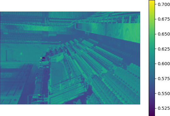
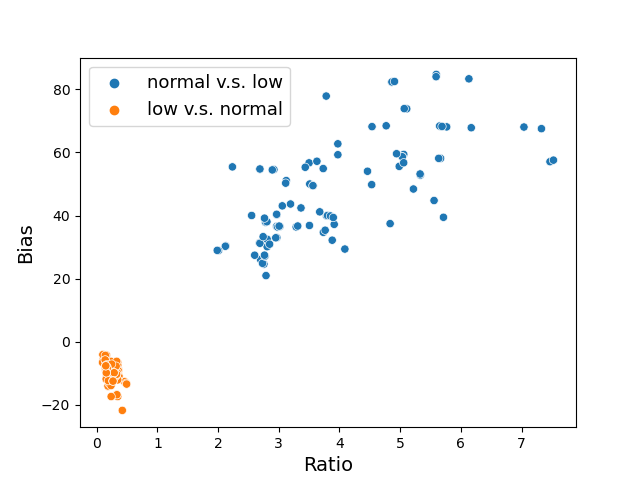
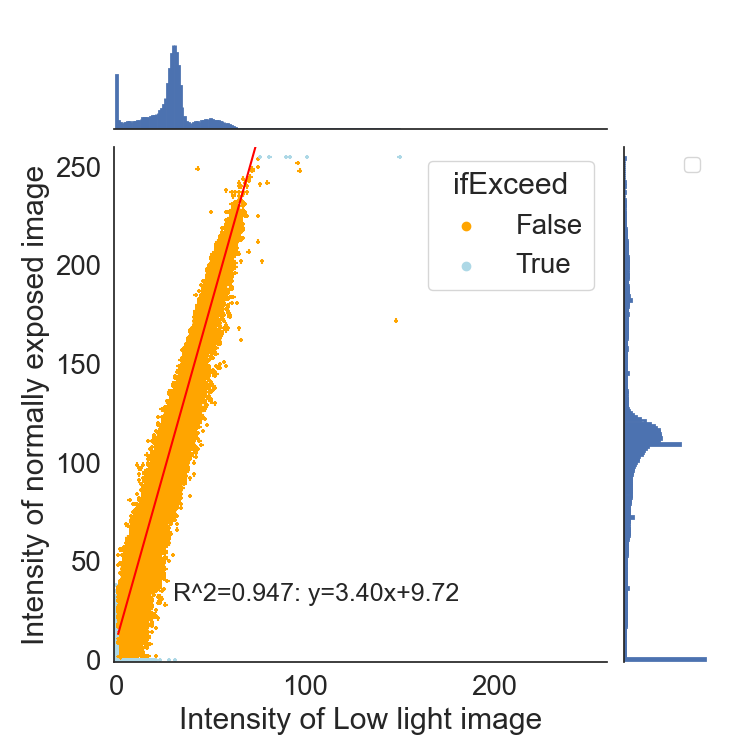
Some may argue that the noise term in Eq. 10 can be regarded as due to the magnitude difference between the signal and the offset term . However, we can show its mean is hardly zero, and a factor of considerably amplifies its variance. The detailed discussion is given in the appendix. We also conduct statistical experiments on a low light and normally exposed image pair from LOL-v1 (Wei et al., 2018). We plot the joint histogram of paired pixels as shown in Fig. 3. The dots in orange are those of and the dots in light blue are those of or representing the pixels may have dynamic range overflow. A linear regression of is done for the dots . The regressed line is plotted in red and its coefficients are attached beside the line. The regression is fitted well by the linear model with a close to 1. From the statistical experiment, we find has a non-neglegible magnitude.
4 Method
Based on the extended DI-Retinex theory, we notice that directly regarding reflectance as the final enhanced result is inappropriate. Similarly, only estimating a single matrix such that the enhanced image is also inaccurate. This is because there exists an offset between the normal image and proportionally enhanced image . Therefore, we adopt a contrast brightness adjustment function involving a flexible offset for efficient enhancement.
4.1 Contrast Brightness Adjustment Function
The algorithm commonly used in brightness adjustment (Fredrik Lundh and Contributors, ) is as follows:
| (12) |
where is a brightness adjustment coefficient ranging from 0 to infinity. When , the image becomes dimmer, and when it turns entirely black. When , the image keep unchanged. When , the image becomes brighter. The algorithm proportionally enhances pixel intensity and thus may generate images with improper contrast.
The algorithm commonly used in contrast adjustment (Fredrik Lundh and Contributors, ) is as follows:
| (13) |
where is a contrast adjustment coefficient ranging from 0 to infinity and is the average intensity of the input image. When equals or , the image becomes a solid gray image or keeps unchanged, respectively. The idea is to enlarge the contrast range of zero mean and then add the average intensity back to make sure the brightness of the image remains unchanged.
However, both Eq. 12 and Eq. 13 cannot adjust contrast and brightness simultaneously. Therefore, a contrast brightness adjustment function (android gpuimage, ) is used as follows:
| (14) |
where and are the factors for contrast and brightness adjustment, respectively. A yields a brighter output and gives a dimmer one. Compared to Eq. 13, a biased average is subtracted from pixel intensity and later a reverse biased one is added back. By Eq. 14, the image can be adjusted in terms of contrast and brightness simultaneously.
Neural networks are known to be good at predicting output with a restricted range, e.g., , while and the unknown range of make network difficult to predict them correctly. Therefore, we first make the restricted within so that the network can learn to predict them better. Through substituting by the half of max pixel value , Eq. 14 can be rewritten
| (15) |
When , Eq. 15 is reduced to , where turns all pixels to max intensity, namely pure white, and makes all pixels non-positive, namely pure black. increases () or reduces () the brightness of image. And enlarges () or reduces () the contrast of image.
The coefficient with range to infinity also hinders the accurate prediction of network. Therefore, a mapping function can be introduced. We have experimented several functions , and empirically found the following one the best.
| (16) |
where is a small number to avoid causing error in program. Based on the function Eq. 15 and mapping function Eq. 16, we propose to use an enhancement network consisting of solely three convolutional layers with parameters to predict pixel-wise coefficients and for efficient contrast brightness adjustment.
| (17) |
where , and . The expression is in line of the proportional relationship in Eq. 10. We design two losses for guiding the parameters and to learn the features of and .


4.2 Reverse Degradation Loss
Though the enhancement based on Eq. 10 has a non-negligible offset, the reverse degradation process transforming to can be approximated to a linear proportion. We can similarly obtain
| (18) | ||||
| where | (19) |
We apply Gamma transformation to Eq. 18 and can obtain . The detailed discussion is attached in the appendix. Therefore, we propose a masked reverse degradation loss as follows:
| (20) |
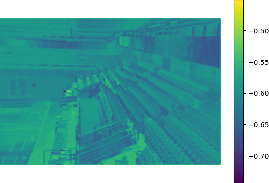
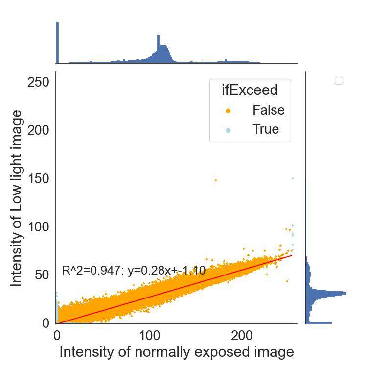
where is the resulting enhanced image based on Eq. 17, with an exposure factor . Based on the finding that the average exposure of a normally exposed image is nearly (Mertens et al., 2007, 2009), is set to . The variance of Gaussian specifies the divergence of targeted exposures, which will be determined in experimental settings. The power of can suppress the magnitude of and its details are discussed in the appendix. We aso plot the joint histogram of vs. as shown in the last plot of Fig. 3. A linear regression of is done for the dots . The regression is fitted well by the linear model with a large . As shown, has a small magnitude and is a negligible offset.
The mask function is defined as
| (21) |
The mask function is introduced because the approximate linear proportion between and is limited in regions without dynamic range compression.
4.3 Variance Suppression loss


We want the second term in Eq. 17 consisting of and to learn the feature of in Eq. 10. We have shown that though has a non-zero mean that yields a necessary offset for modeling enhanced images, it has an amplified variance due to , which will contribute to an enhanced variance of recovered images. Therefore, we design a variance suppression loss such that its variance approaches zero. The expression of the variance suppression loss is given by
| (22) |
where is computed along each channels. As a result, the overall loss of our model is as follows:
| (23) |
4.4 Relation between DI-Retinex and the enhancement model
The traditional Retinex theory, originally borrowed from optics, has served as a fundamental guiding principle for numerous prior low-light enhancement works. However, it has come to our attention that the digital imaging process introduces deviations from the optical Retinex theory, resulting in the emergence of what we term the DI-Retinex theory. In accordance with this novel theory, we derive Eq. 10, wherein emerges as a significant term. In contrast, if we were to rely solely on the conventional Retinex theory, would assume a value of zero. This, in turn, renders the subsequently derived enhancement model in Eq. 17, which incorporates an offset term, invalid. In summary, the proposed DI-Retinex theory ensures the presence of a non-negligible offset term in the relationship between low-light and normal images. This, in turn, substantiates the formulation of the presented enhancement model, which features an offset term. Furthermore, the DI-Retinex theory establishes a reverse relationship between low-light and normal images, enabling us to derive the reverse degradation loss.
5 Experiments
5.1 Experimental Settings
Datasets. We adopt the datasets for comparison including LOL-v1 (Wei et al., 2018), LOL-v2 (Yang et al., 2021b), and DARKFACE (Yuan et al., 2019). The details and statistics of the datasets are illustrated in the supplemental material. The number of training and test sets of LOL-v1 (Wei et al., 2018), LOL-v2-Real (Yang et al., 2021b) and DARKFACE (Yuan et al., 2019) are illustrated in Table. 1. We randomly sample 1000 images for DARKFACE following (Li et al., 2021a; Ma et al., 2022). Note that LOL-v2 has a synthetic part and a real captured part. Since we are modeling realistic low light degradation by extended Retinex theory, we only experiment on its real part.
| Train | Test | |
| LOL-v1 | 485 | 15 |
| LOL-v2-Real | 689 | 100 |
| DARKFACE | # of Images | # of Faces |
| 1000 | 37040 |


Baselines. We compare our methods with model-based method including LIME (Guo et al., 2016), supervised learning methods including RetinexNet (Wei et al., 2018), KinD (Zhang et al., 2019b), and RUAS (Liu et al., 2021), semi-supervised learning methods including DRBN (Yang et al., 2021a), unpaired supervised learning methods including EnlightenGAN (Jiang et al., 2021) and NightEnhance (Jin et al., 2022), and zero-shot learning methods including RRDNet (Zhu et al., 2020a), Zero-DCE (Guo et al., 2020), Zero-DCE++ (Li et al., 2021b), RetinexDIP (Zhao et al., 2021), SCI (Ma et al., 2022) and PairLIE (Fu et al., 2023b). Since our method belongs to zero-shot learning, we focus on the comparison with the existing zero-shot learning methods.
| MSE | PSNR | SSIM | LPIPS | |
| Input | 12.622 | 7.771 | 0.181 | 0.560 |
| LIME (Guo et al., 2016) | 2.269 | 16.760 | 0.560 | 0.350 |
| RetinexNet (Wei et al., 2018) | 1.656 | 16.774 | 0.462 | 0.474 |
| KinD (Zhang et al., 2019b) | 1.431 | 17.648 | 0.779 | 0.175 |
| RUAS (Liu et al., 2021) | 3.920 | 16.398 | 0.537 | 0.350 |
| DRBN (Yang et al., 2021a) | 2.359 | 15.125 | 0.472 | 0.316 |
| EnlightenGAN (Jiang et al., 2021) | 1.998 | 17.478 | 0.677 | 0.322 |
| RRDNet (Zhu et al., 2020a) | 6.313 | 11.384 | 0.470 | 0.361 |
| RetinexDIP (Zhao et al., 2021) | 6.050 | 11.646 | 0.501 | 0.317 |
| ZeroDCE (Guo et al., 2020) | 3.282 | 14.857 | 0.589 | 0.335 |
| ZeroDCE++ (Li et al., 2021b) | 3.035 | 15.342 | 0.603 | 0.316 |
| SCI (Li et al., 2021b) | 3.496 | 14.780 | 0.553 | 0.332 |
| NightEnhance (Jin et al., 2022) | 1.070 | 21.521 | 0.763 | 0.235 |
| PairLIE (Fu et al., 2023b) | 1.419 | 18.463 | 0.749 | 0.290 |
| Ours | 0.784 | 21.542 | 0.766 | 0.219 |
| Ours (small) | 1.706 | 18.448 | 0.641 | 0.312 |
Evaluation Criteria. We employ four full-reference metrics, i.e., MSE, PSNR, SSIM (Wang et al., 2004) and LPIPS (Zhang et al., 2018), and two metrics indicating efficiency, i.e., model size and inference time. For the dataset DARKFACE (Yuan et al., 2019), a Precision-Recall curve is plotted for performance indication.
Implementations. We train our model on the training set of each dataset. We use ADAM as the optimizer with an initial learning rate of and weight decay of . The variance of Gaussian distribution in the reverse degradation loss is set to and in Eq. 16 is set to 0.2. The network is trained for epochs. Since the network is small and learns mapping coefficients and globally, we do not crop patches during training. Batch size is set to . All experiments are conducted on an NVIDIA GeForce GTX 1080 GPU and implemented by PyTorch (Paszke et al., 2019). Our codes will be released.

5.2 Results on LOL-v1
We first evaluate our method on LOL-v1 (Wei et al., 2018) by comparing its LLIE performance with other existing methods. The quantitative results are shown in Table. 2. We can see that our model has the best performance in terms of MSE and PSNR. Furthermore, our method has the second-best value of SSIM and LPIPS. We also train another small version of our model by reducing internal (64 to 4) and output channels (6 to 2). The performance of our small model can still outperform most existing methods. Note that the number of parameters in our model is only of PairLIE (Fu et al., 2023b), of NightEnhance (Jin et al., 2022) and of KinD (Zhang et al., 2019b).
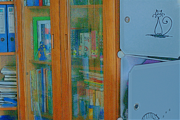
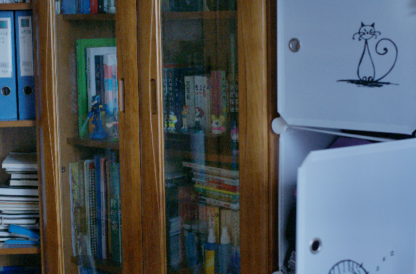
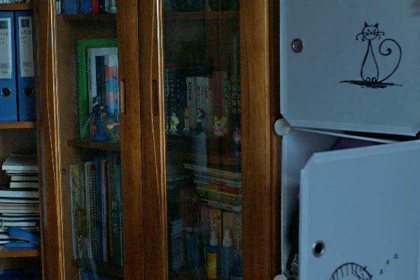
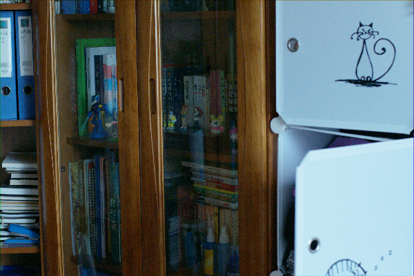
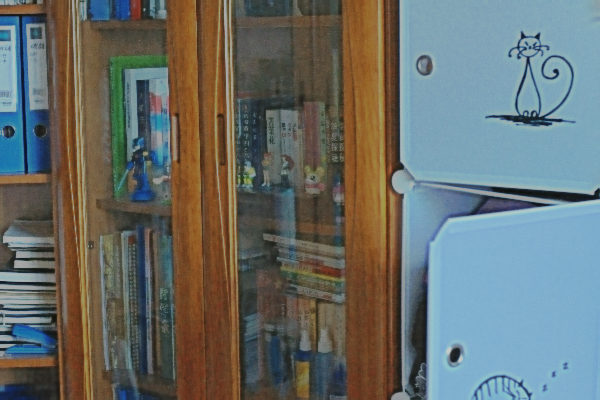
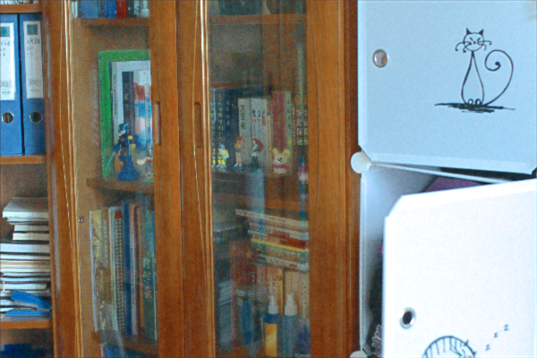
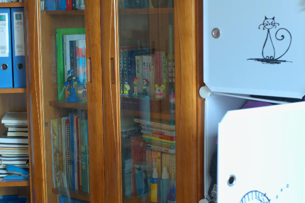
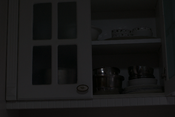
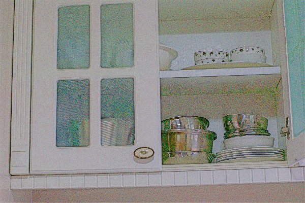
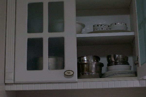
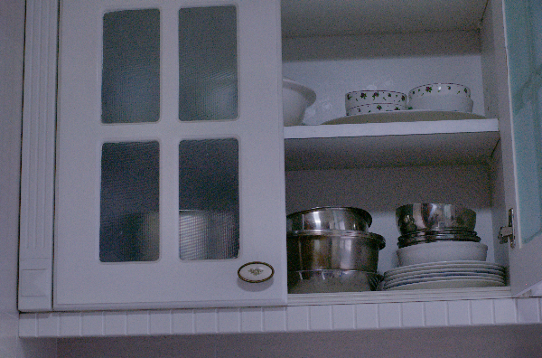
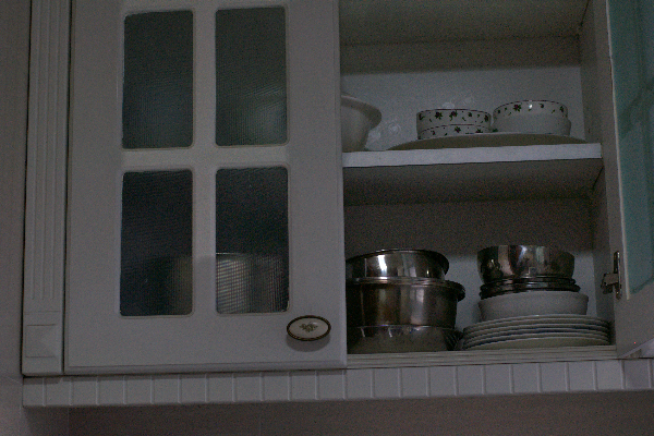
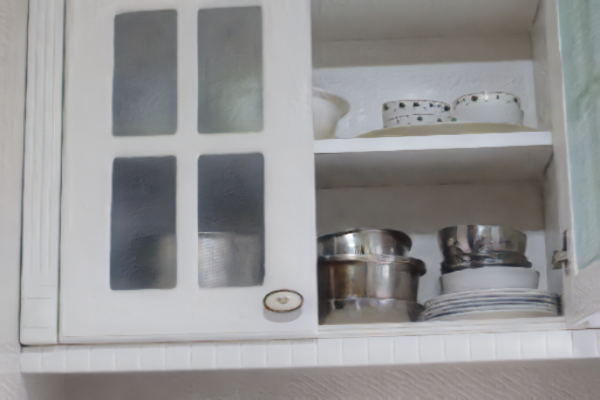
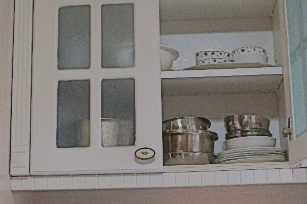
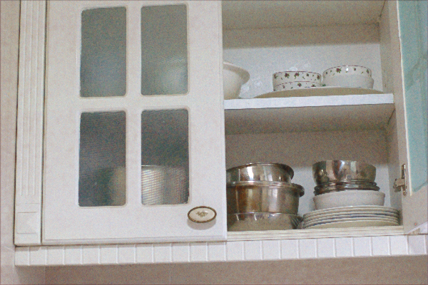
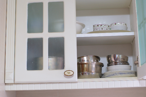
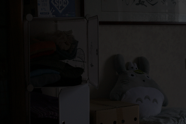
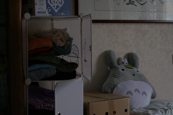
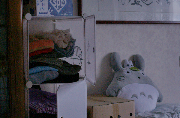
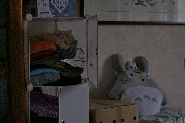
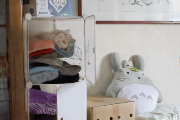
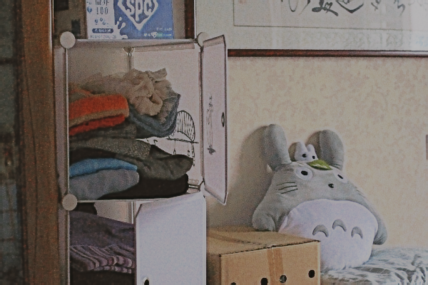
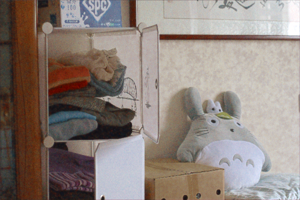
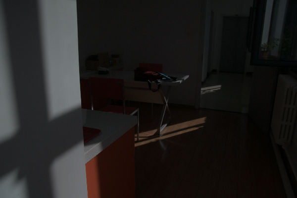
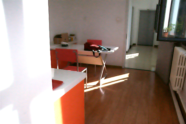
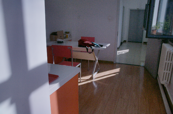
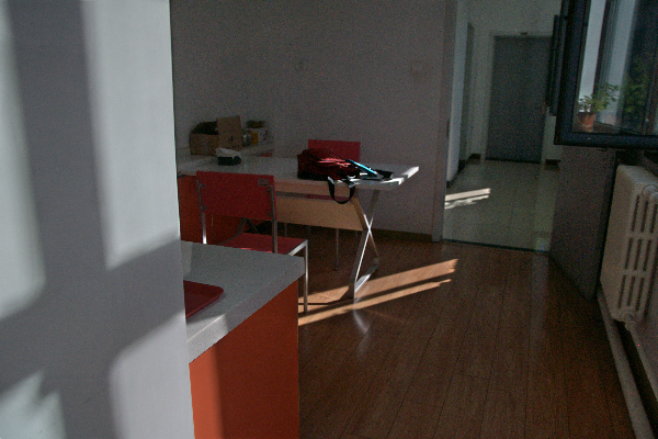
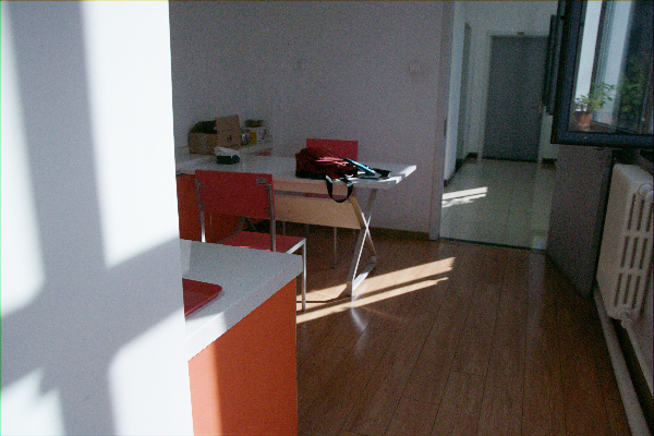
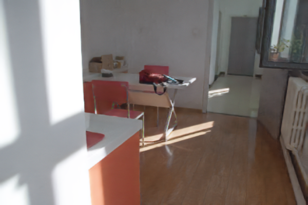
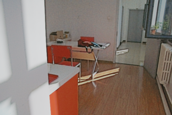
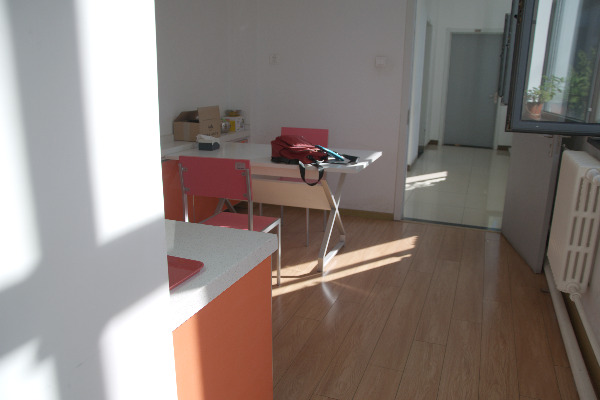
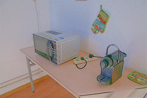
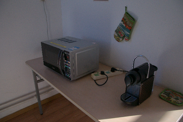
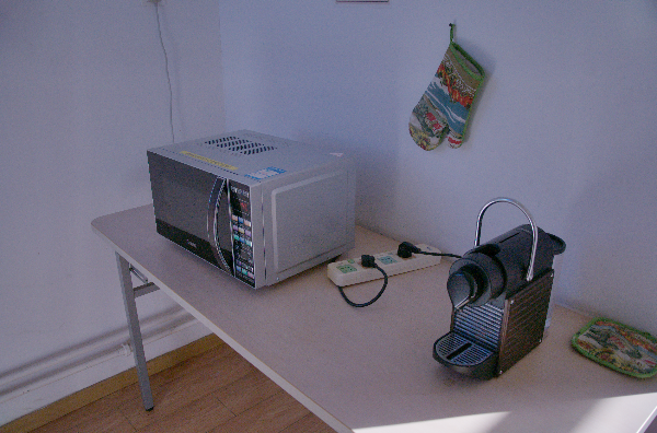
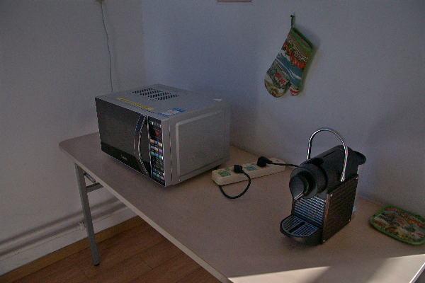
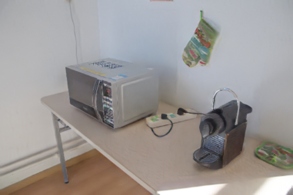
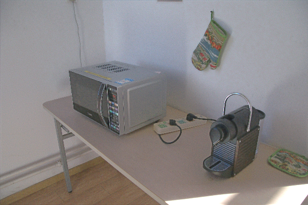
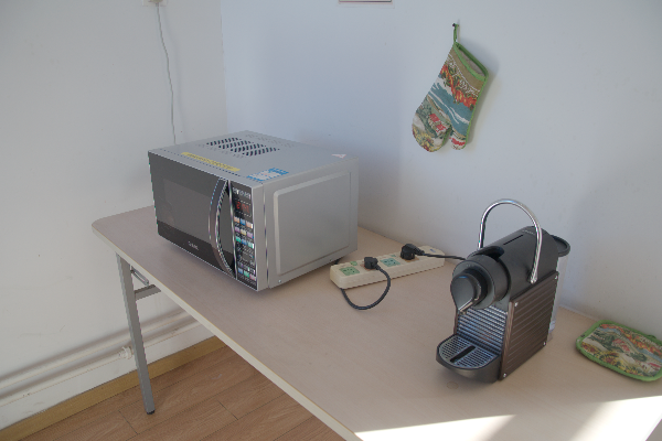
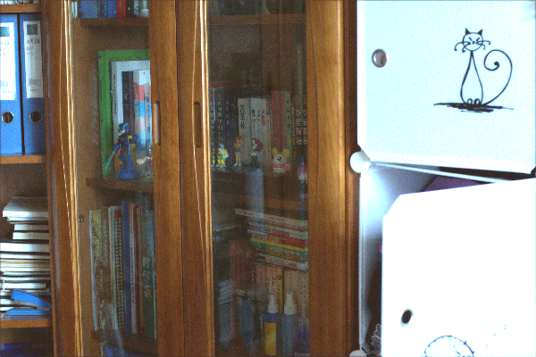
We then give several examples for the visual comparison among the existing methods and ours in Fig. 4 to Fig. 6. We can see in Fig. 4 that only our model restores the contents in the bookshelf. In addition, in the pure white region in the bottom right corner, other methods are “afraid” of enhancing the white pixels, which are meant to be overexposed in photography, towards overexposure. However, our proposed mask function in deals with the dynamic range overflow and enables the successful enhancement of the white pixels. In Fig. 5, most methods cannot recover the brightness of the imaging scene properly except NightEnhance (Jin et al., 2022) and ours. Compared with NightEnhance (Jin et al., 2022), our method better enhances the shadow inside the cupboard. In Fig. 6, still only ours and NightEnhance (Jin et al., 2022) can achieve the closest results to the ground-truth. However, our method restores the color of the wall with more vivid fidelity.
5.3 Results on LOL-v2
| MSE | PSNR | SSIM | LPIPS | |
| Input | 7.634 | 9.718 | 0.190 | 0.333 |
| LIME (Guo et al., 2016) | 1.484 | 15.240 | 0.470 | 0.360 |
| RetinexNet (Wei et al., 2018) | 1.719 | 15.470 | 0.560 | 0.421 |
| KinD (Zhang et al., 2019b) | 4.029 | 14.740 | 0.641 | 0.302 |
| RUAS (Liu et al., 2021) | 2.540 | 15.330 | 0.520 | 0.322 |
| DRBN (Yang et al., 2021a) | 1.843 | 19.600 | 0.764 | 0.246 |
| EnlightenGAN (Jiang et al., 2021) | 1.209 | 18.230 | 0.610 | 0.309 |
| RRDNet (Zhu et al., 2020a) | 3.594 | 14.850 | 0.560 | 0.265 |
| RetinexDIP (Zhao et al., 2021) | 3.157 | 14.513 | 0.546 | 0.274 |
| ZeroDCE (Guo et al., 2020) | 1.777 | 18.059 | 0.605 | 0.298 |
| ZeroDCE++ (Li et al., 2021b) | 1.569 | 18.491 | 0.617 | 0.290 |
| SCI (Ma et al., 2022) | 2.132 | 17.304 | 0.565 | 0.286 |
| NightEnhance (Jin et al., 2022) | 0.819 | 20.850 | 0.724 | 0.329 |
| PairLIE (Fu et al., 2023b) | 0.916 | 19.885 | 0.778 | 0.282 |
| Ours | 0.827 | 21.362 | 0.795 | 0.225 |
| Ours (small) | 1.064 | 20.631 | 0.739 | 0.252 |
Similar to LOL-v1 (Wei et al., 2018), we evaluate our method on LOL-v2 (Yang et al., 2021b). The quantitative results are shown in Table. 3. We can see that our model has the best performance in terms of PSNR, SSIM, and LPIPS. The performance of our model with smaller size is the third best in terms of all the metrics.
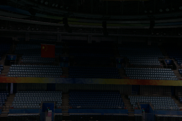
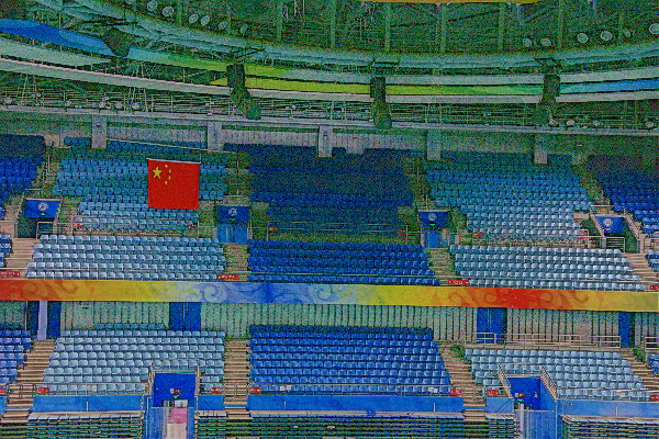
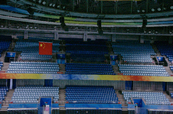
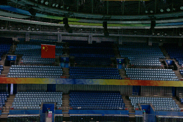
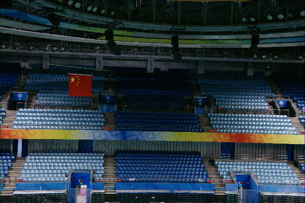
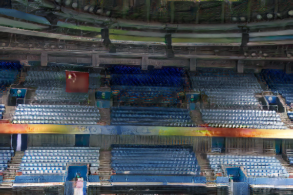
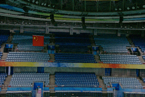
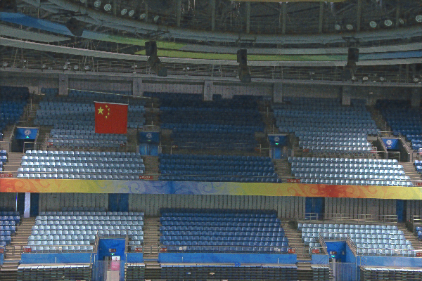
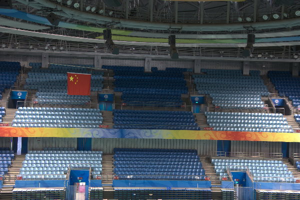
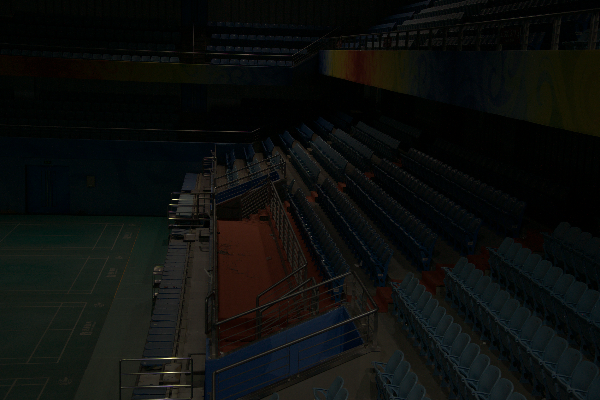
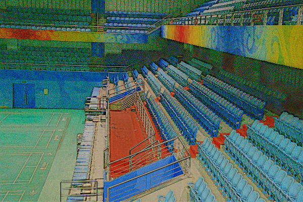
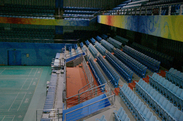
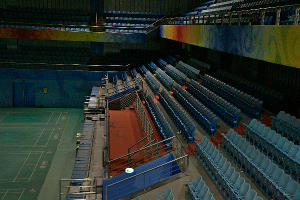
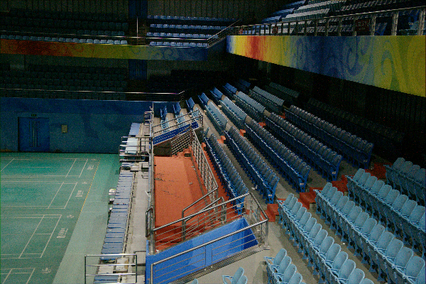
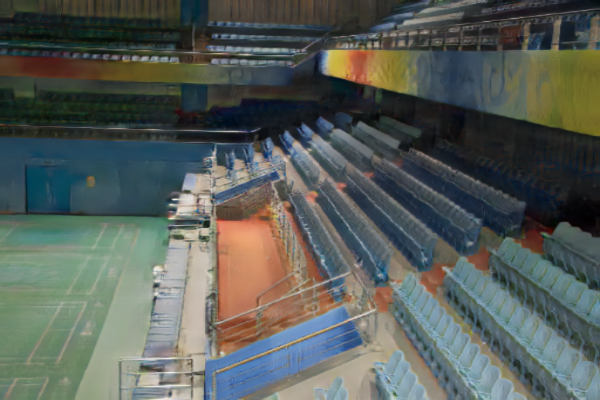
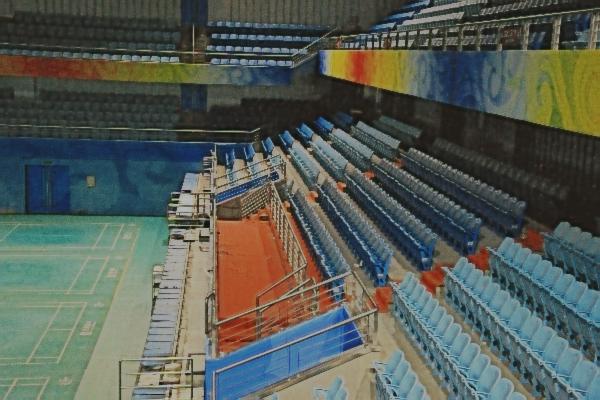
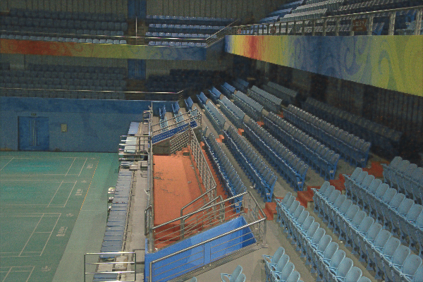
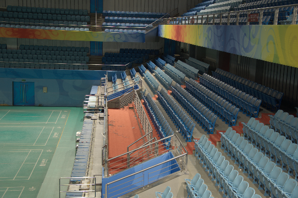
We also provide several illustrative examples for visually comparing our method and others in Fig. 7 to Fig. 10 sampled from LOL-v2 (Yang et al., 2021b). The non-uniform brightness in the grandstand of stadium is challenging for all LLIE methods. Among them, ours and NightEnhance (Jin et al., 2022) can generate the closest results to the ground-truth. However, NightEnhance (Jin et al., 2022) makes the red flag fade, while ours restore the color better. In Fig 9, only our solution yilelds the correct brightness of the white wall. In Fig. 8 and Fig. 10, our method gives the closest results to the ground-truth.

5.4 Ablation Study
We evaluate the effect of the proposed offset , the variance suppression loss , the reverse degradation loss , and the mask function in . We also conduct ablation studies on the choice of scalar or matrix of predicted parameters. We also trial other formulations of the mapping function besides Eq. 16. The expressions are listed below in Eq. 24.
| (24) |
where is a small value preventing error in program. The explanation for choosing the formulations are discussed in the appendix.
The results are shown in Table. 4. We can conclude that each of , , , and leads to better enhancement. The constant parameters cannot fully encode the complex expressions of the coefficients. We show an example in Fig. 11 and the heatmap of decomposed parameters in Fig. 19 in the Appendix. For different choices of the mapping function, has the comparable performance to . However, the double non-linearity of and in yields slower speed and thus we choose in Eq. 16.
| w/o | w/o | w/o | w/o | |
| PSNR | 10.44 | 20.15 | 17.62 | 21.52 |
| SSIM | 0.476 | 0.721 | 0.656 | 0.757 |
| Ours | ||||
| PSNR | 17.43 | 20.34 | 21.62 | 21.54 |
| SSIM | 0.679 | 0.724 | 0.768 | 0.766 |
| FPS | 986 | 891 | 831 | 954 |
| PSNR | 14.29 | 17.78 | 19.40 | 21.54 |
| SSIM | 0.547 | 0.653 | 0.692 | 0.766 |
5.5 Extentions
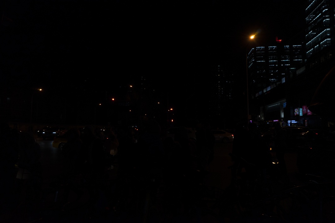
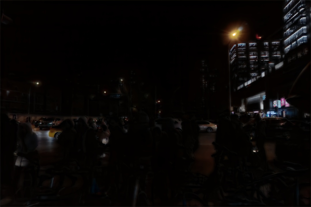
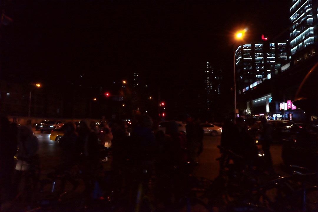
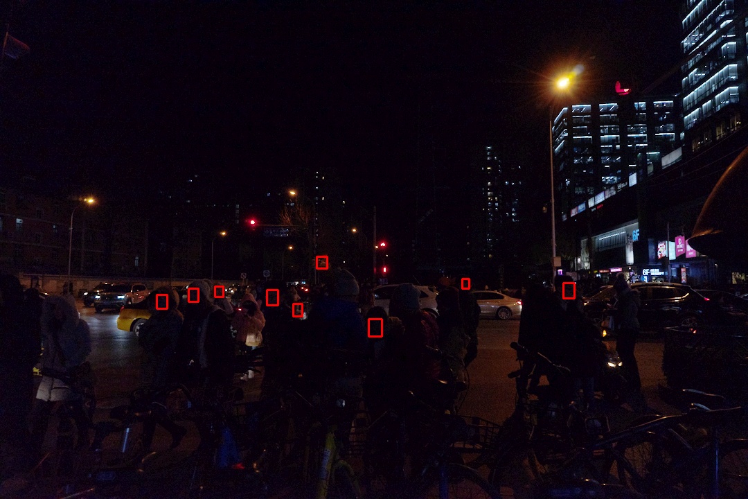
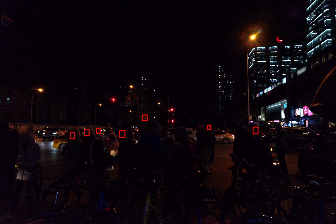
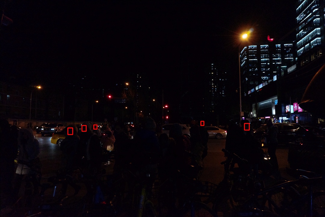
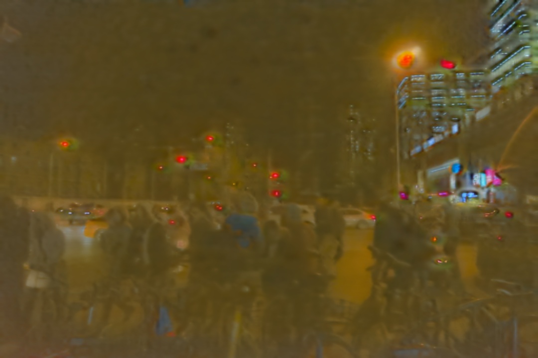
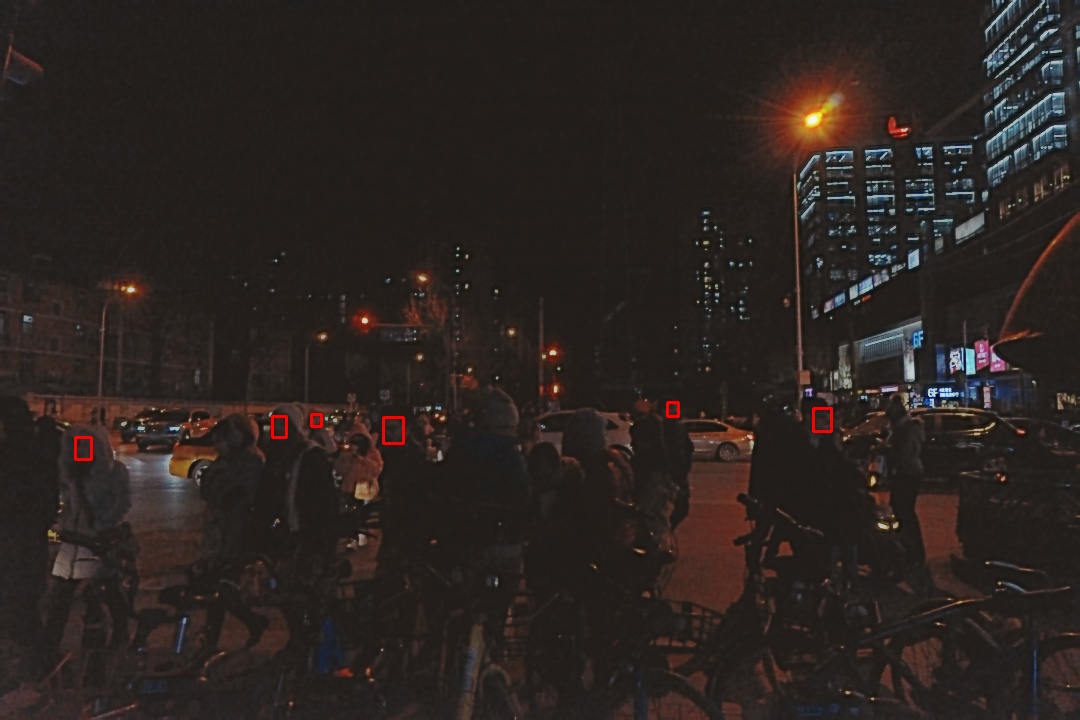
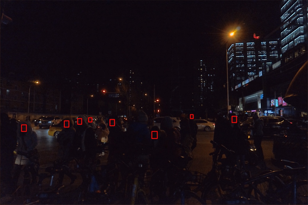
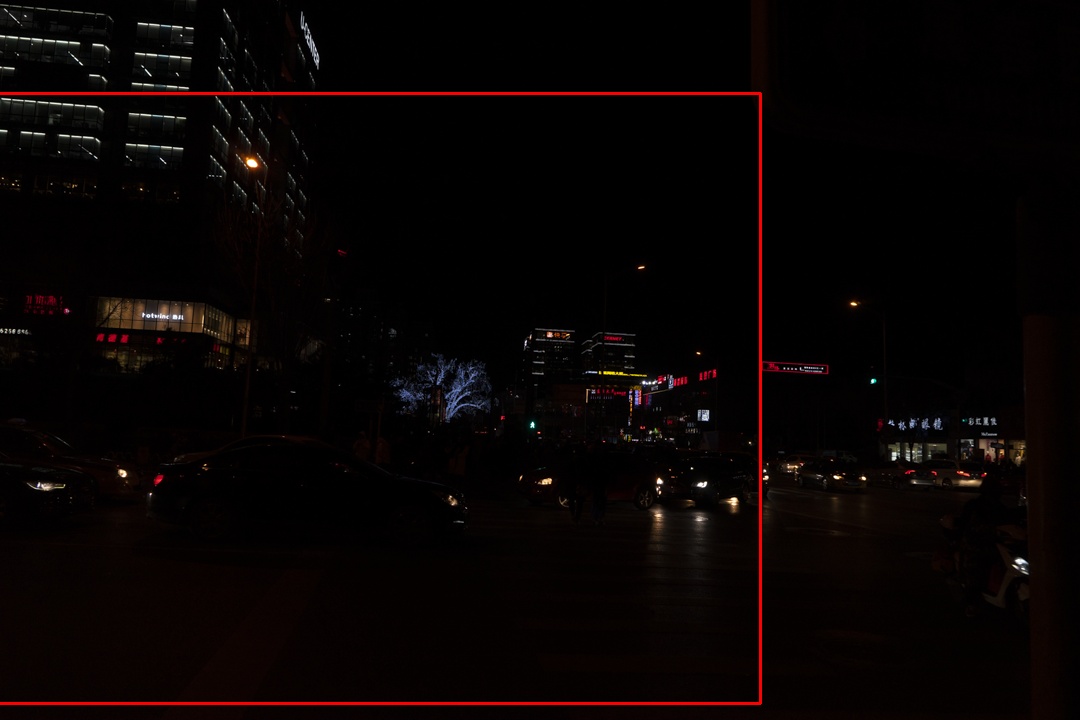
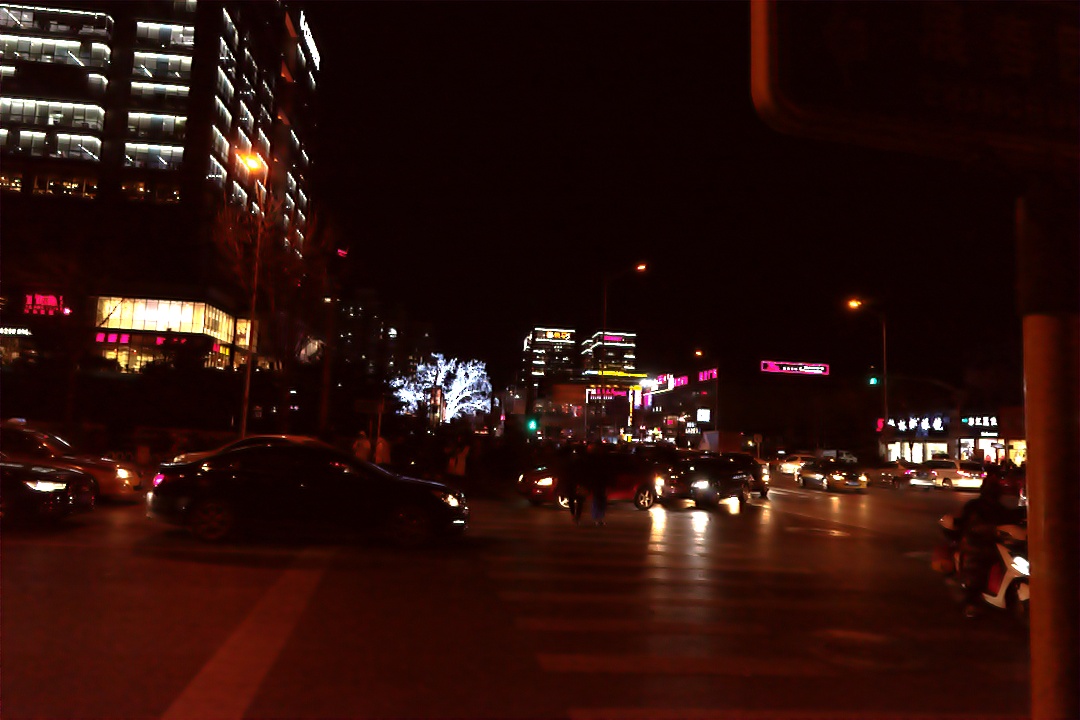
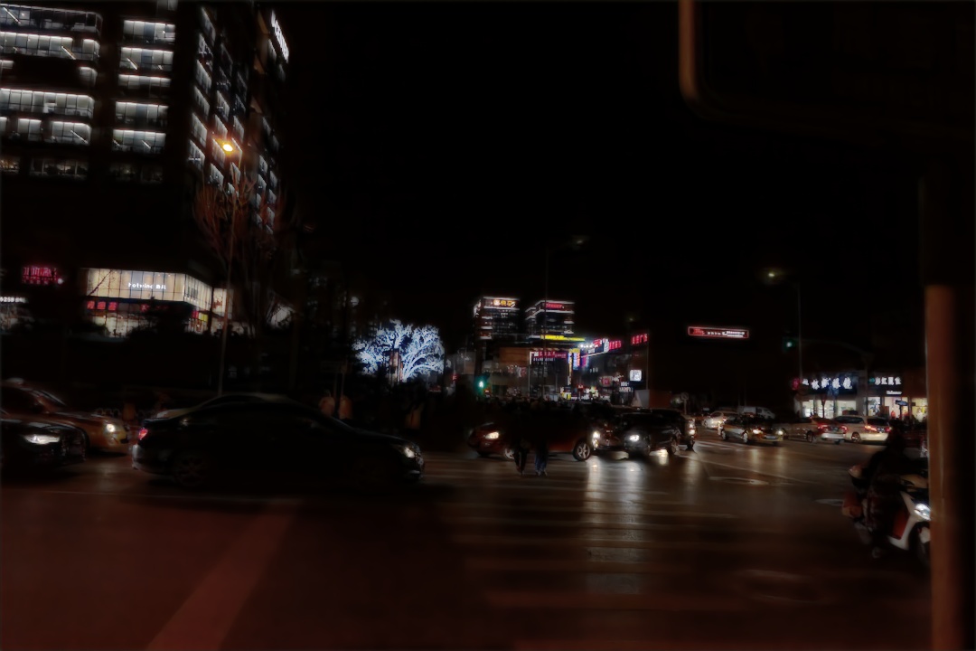
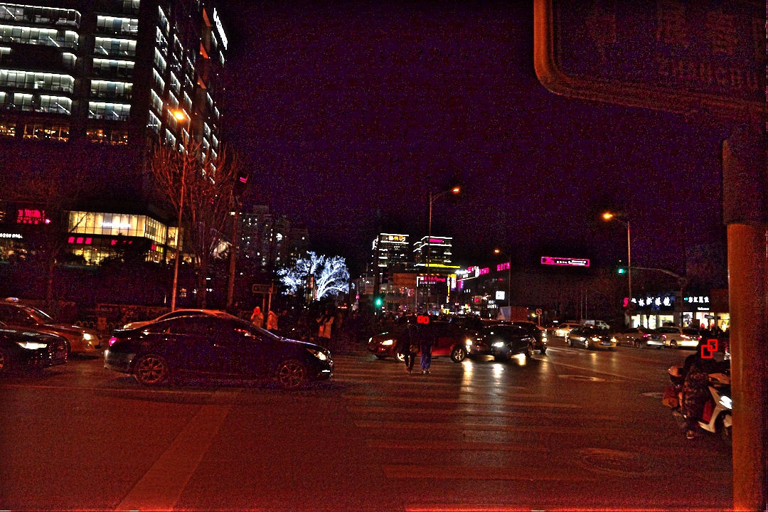
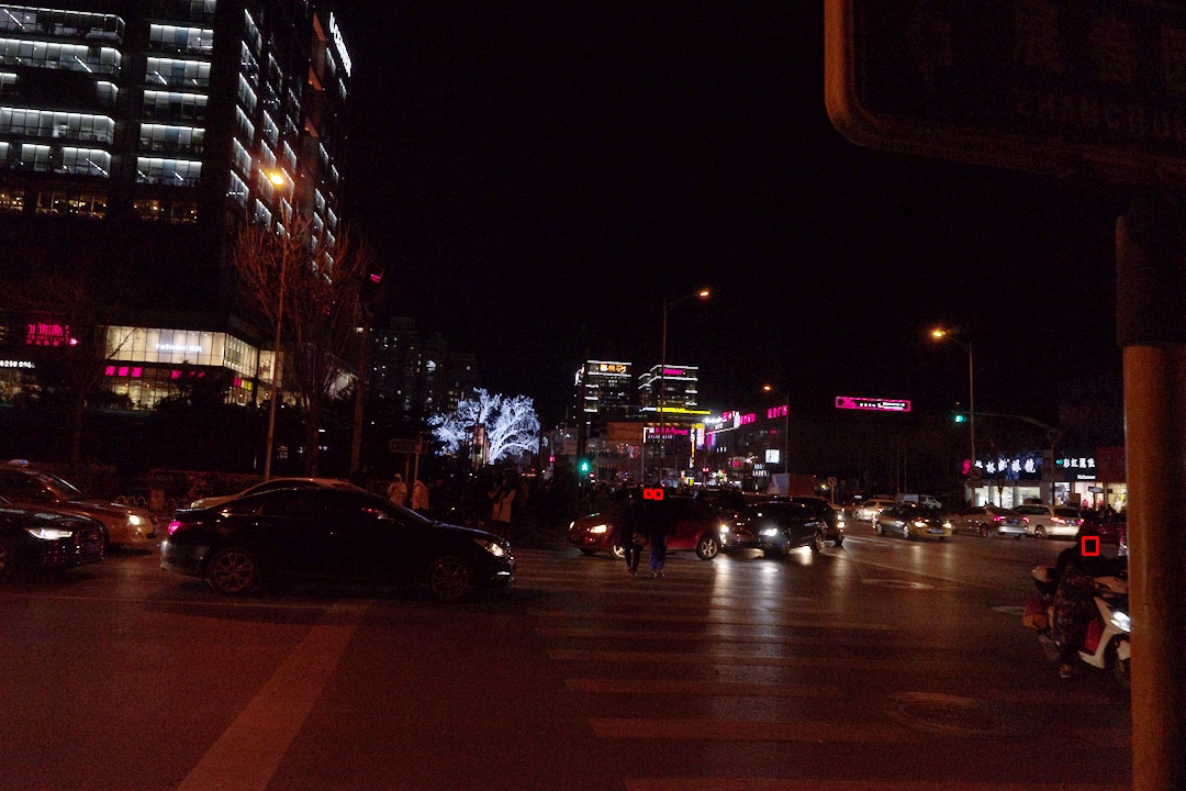
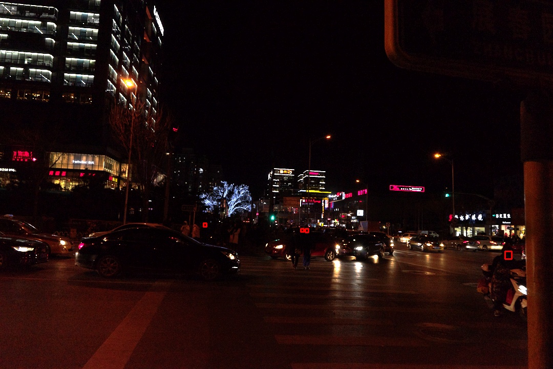
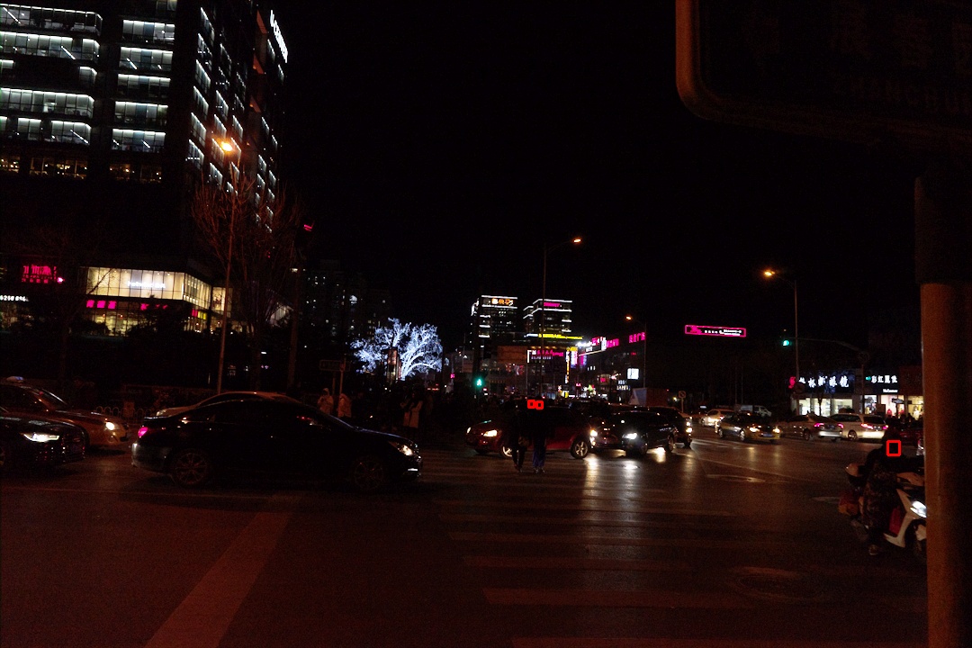
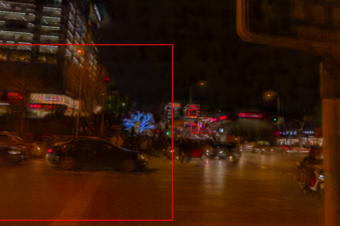
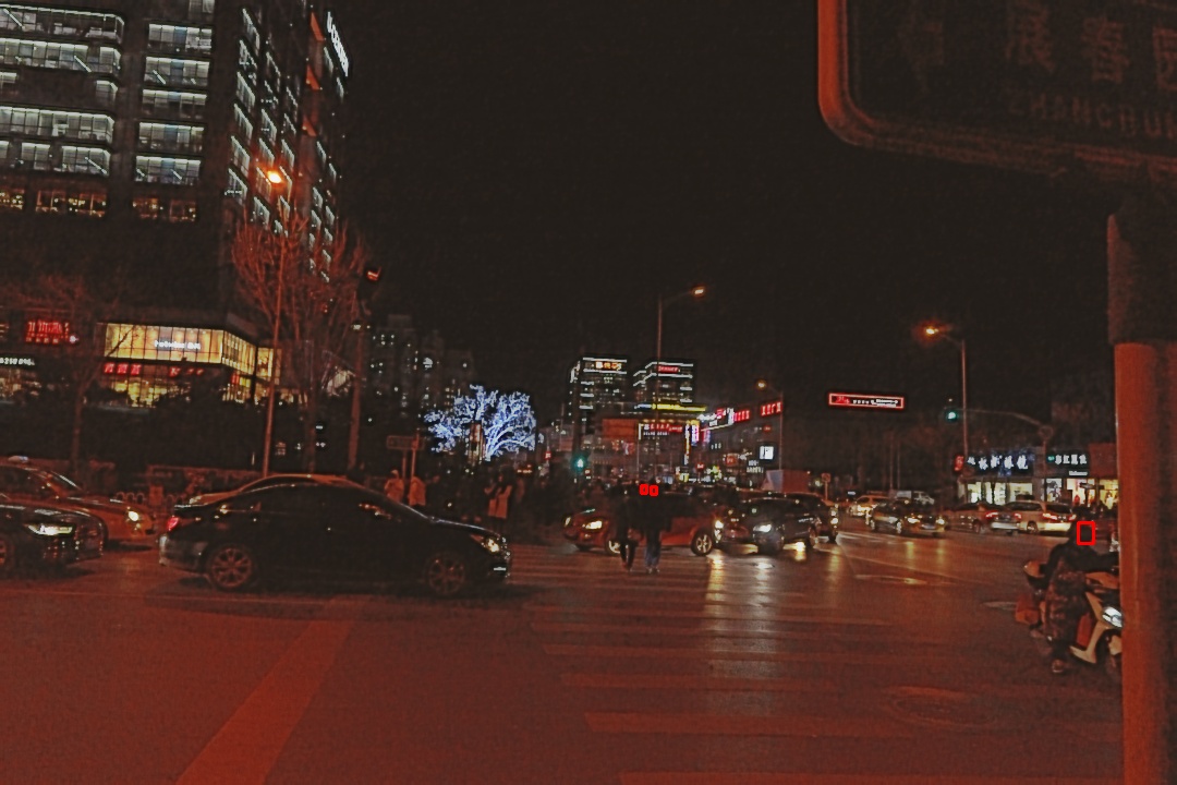
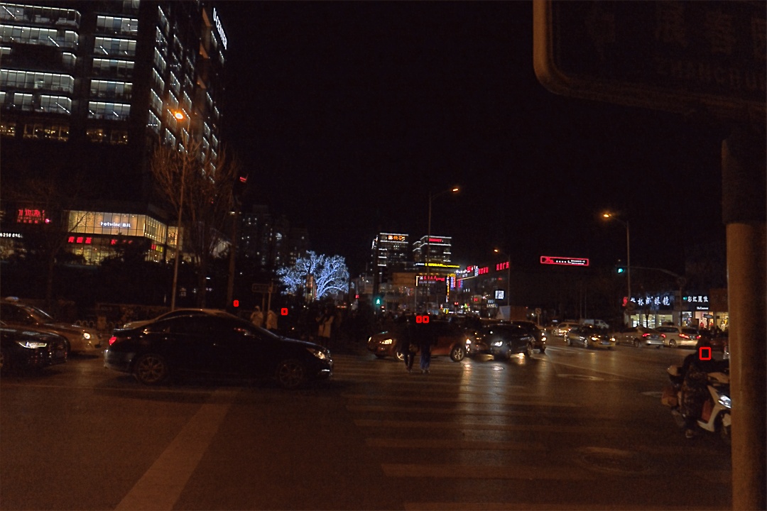
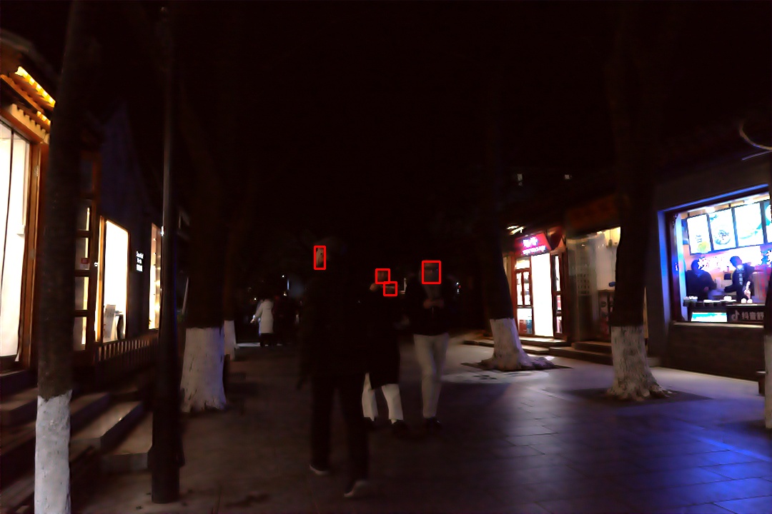
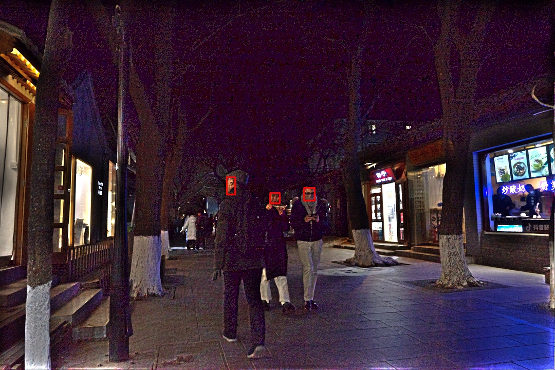
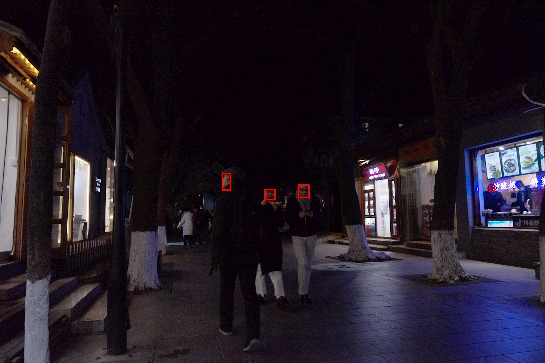
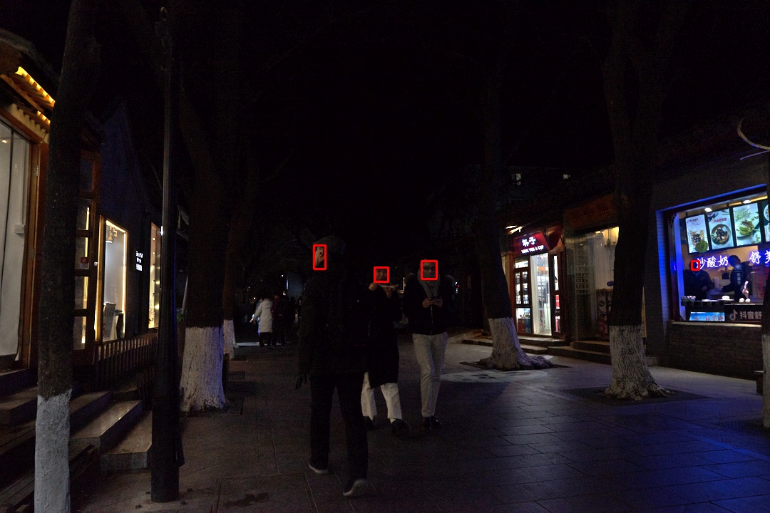
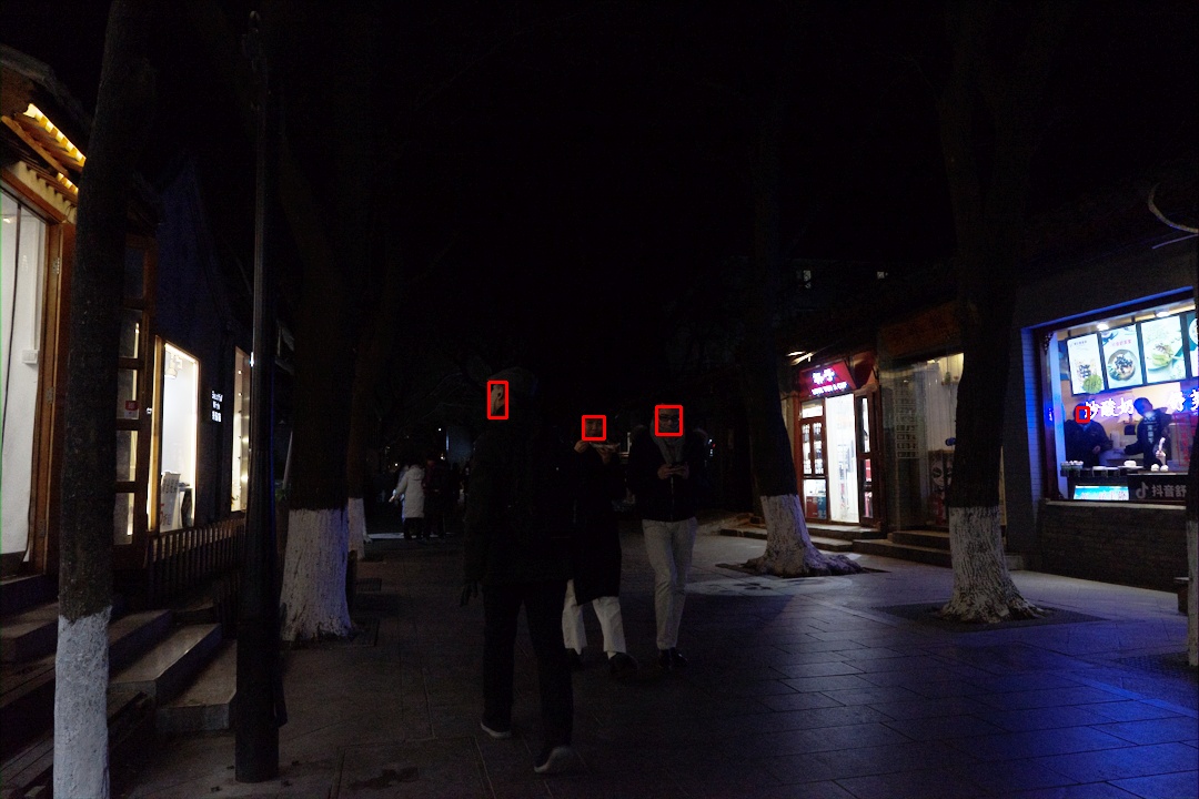
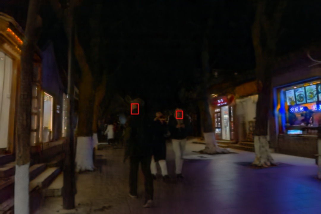
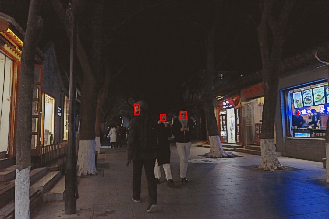
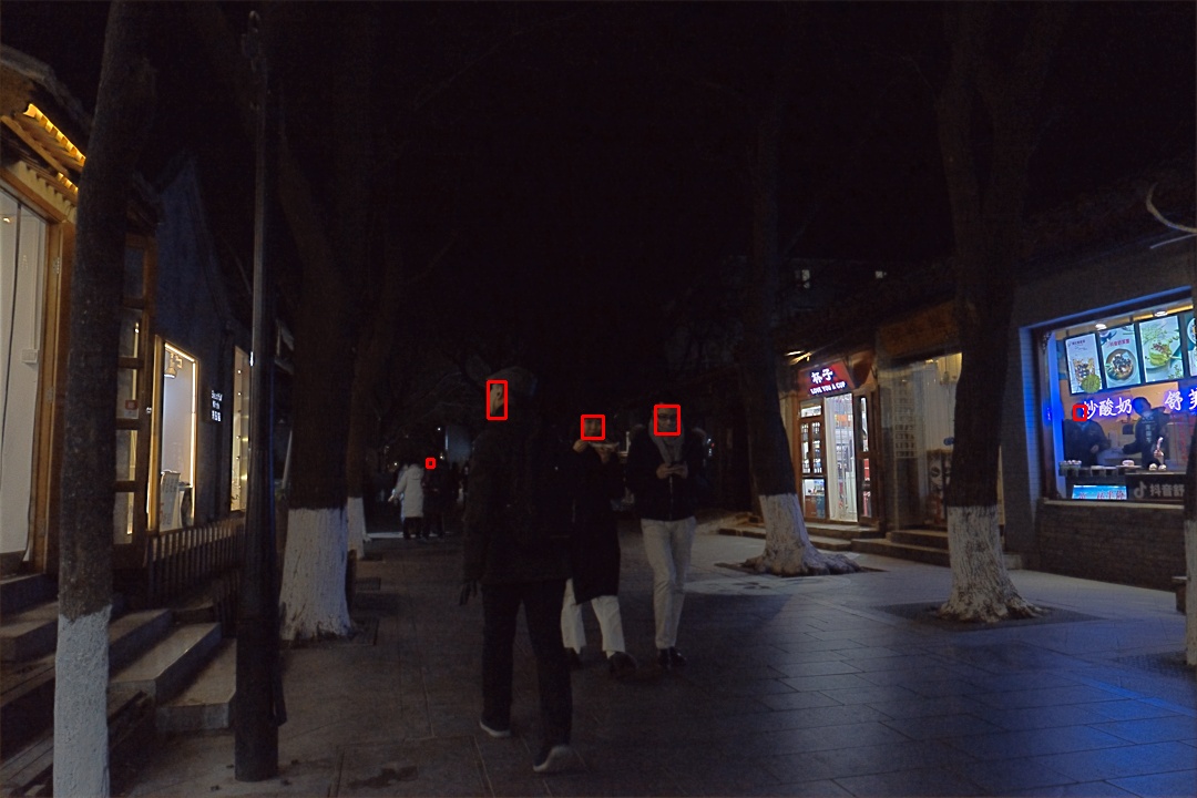
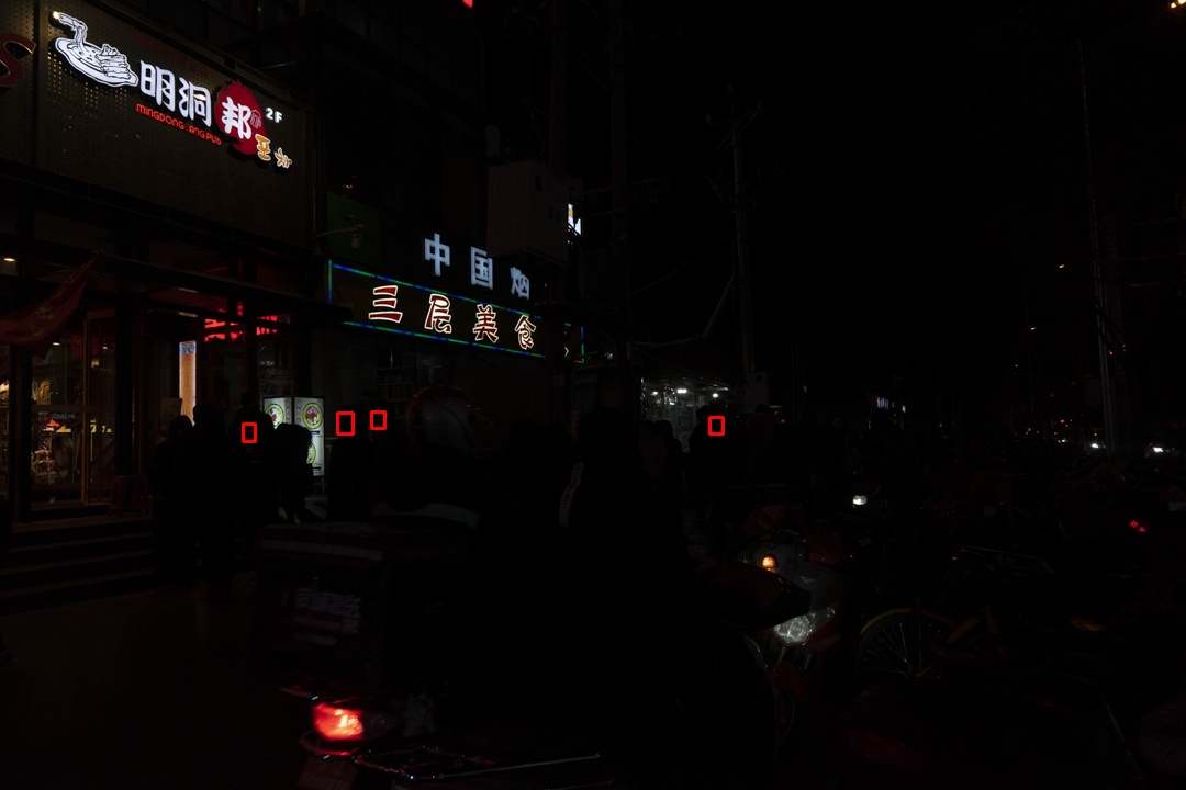
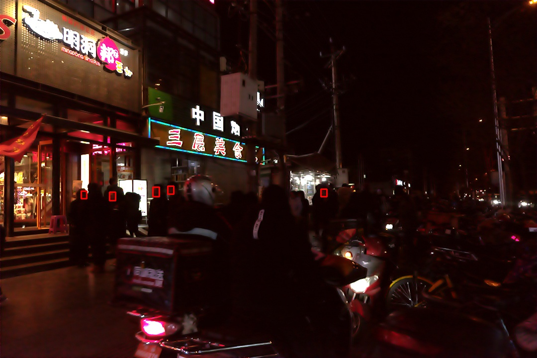
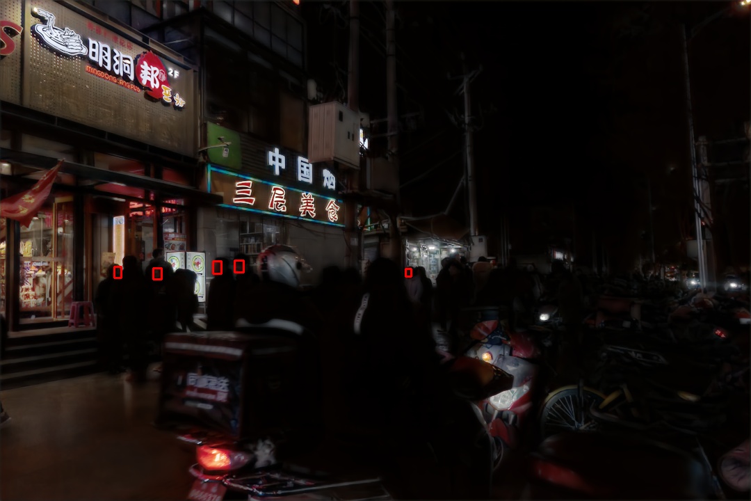
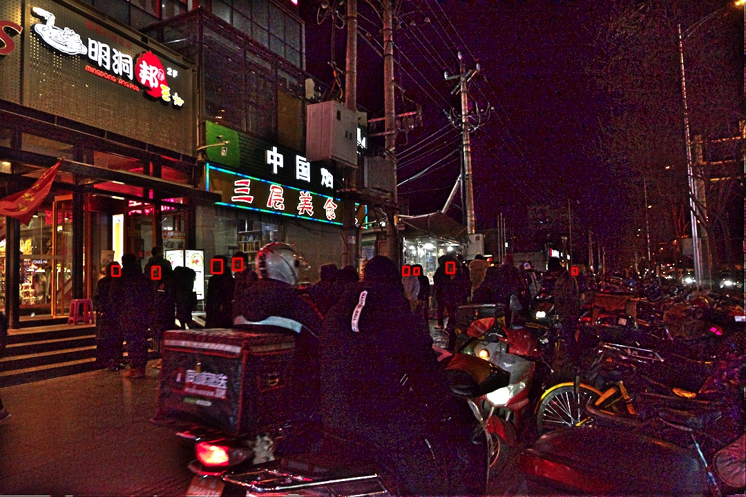
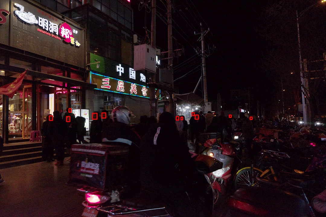
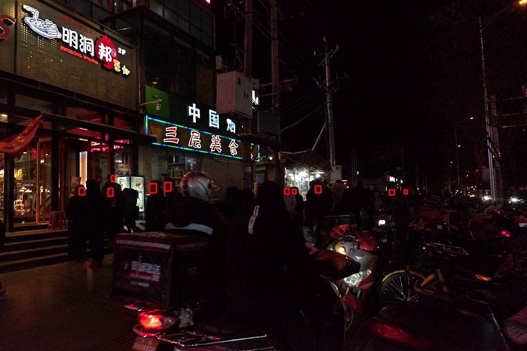
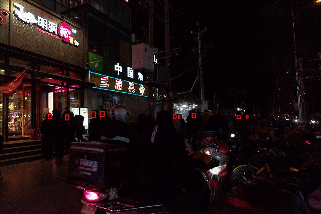
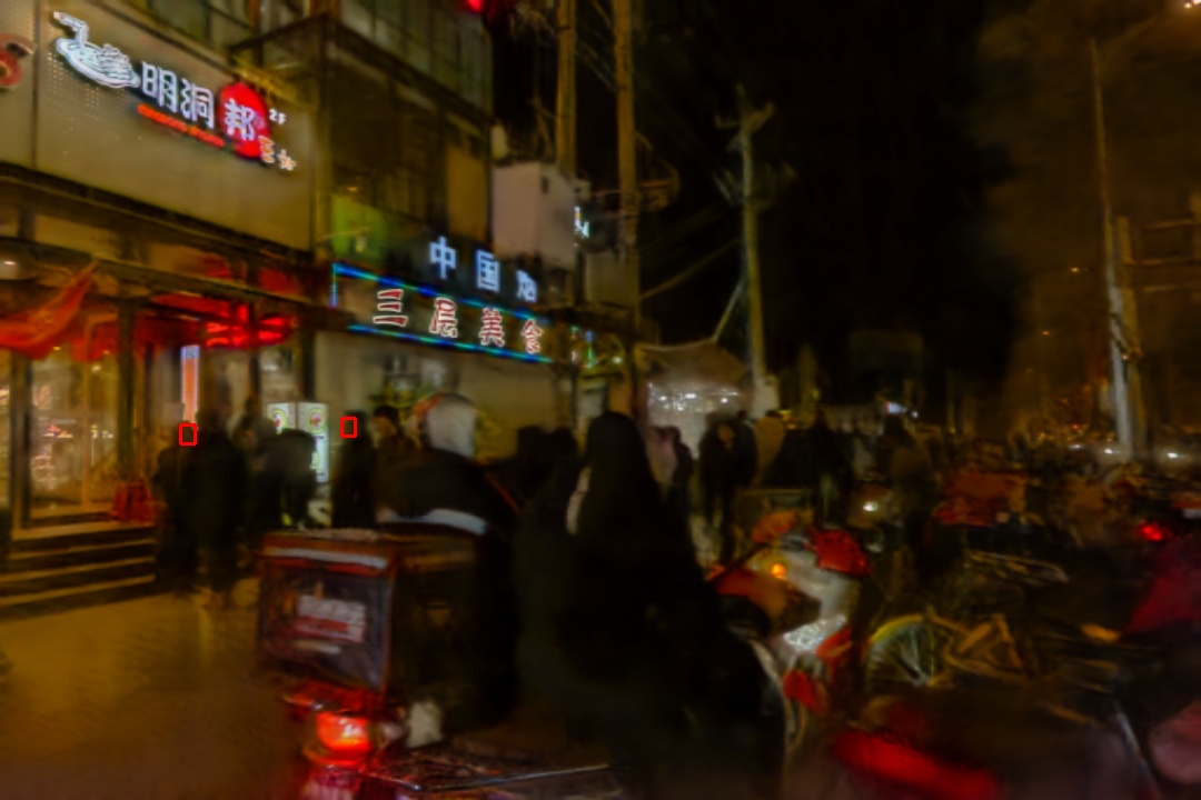
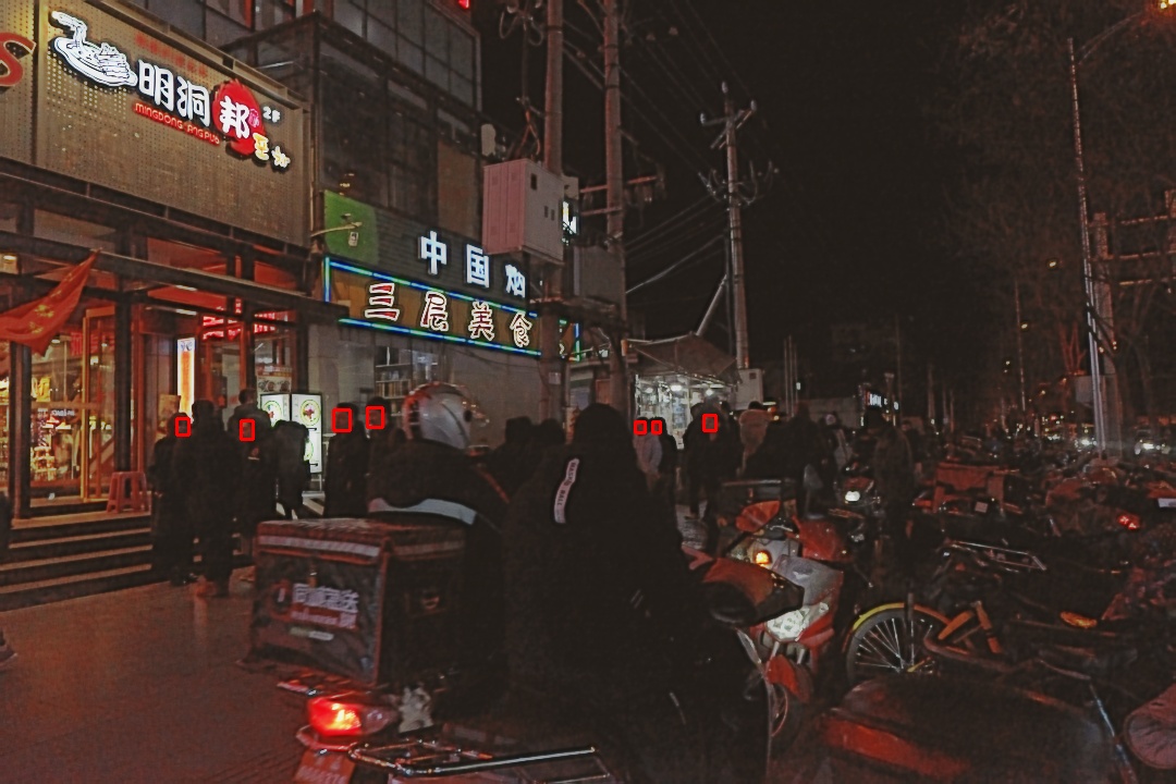
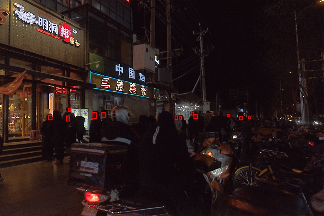
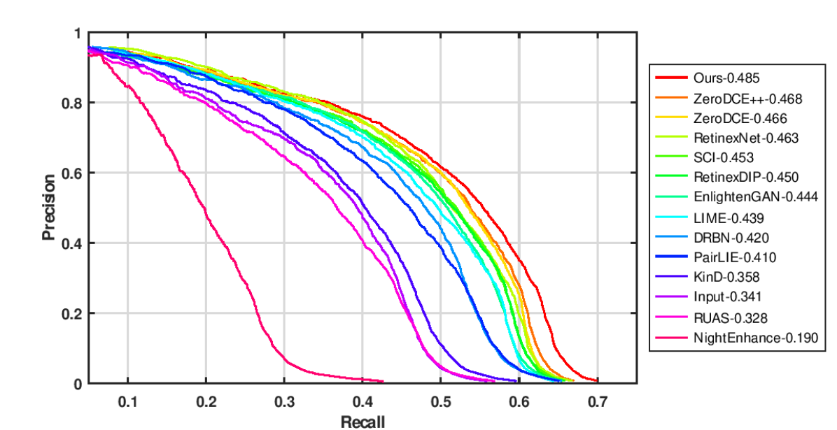
Results on DARKFACE. Image enhancement can serve as a preprocessing for high-level downstream tasks. We thus evaluate our method on a face detection dataset in low-light conditions, i.e., DARKFACE (Yuan et al., 2019). The detector of Dual Shot Face Detector (DSFD) (Li et al., 2019) pretrained on WIDERFACE (Yang et al., 2016) is used for predicting face location. For the enhanced data through each LLIE method, a Precision-Recall curve (PR curve) can be drawn. The stacked PR curves for all methods are shown in Fig. 16. We can see our method has the best performance. Four samples for visual comparison is illustrated in Fig. 12 to Fig. 15, where only the enhancement by our method detects the most faces correctly. Note that though some methods like NightEnhance (Jin et al., 2022) could generate brighter scenes, the introduction of more artifacts and noise reduces the face detection accuracy, which is not consistently in line with human intuition.
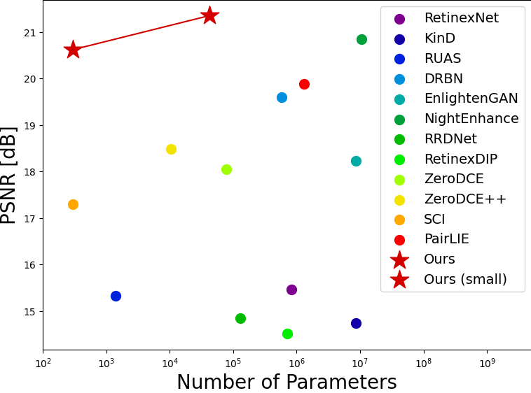
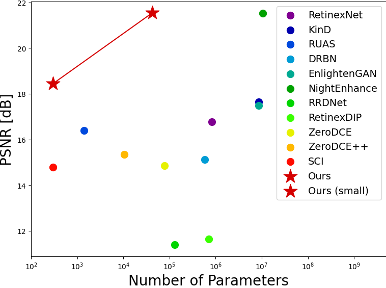
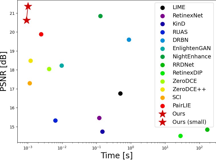
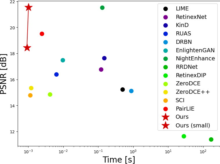
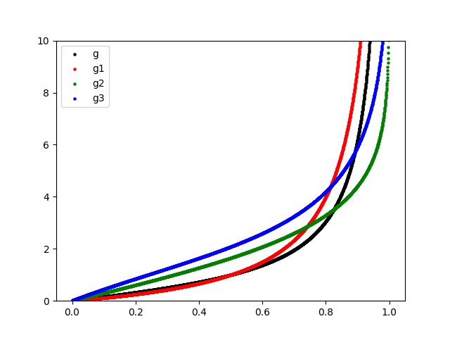
Efficiency. As shown in Fig. 1, our methods achieve the best overall balance between visual quality and model size/run time consistently on LOL-v1 (Wei et al., 2018) and LOL-v2 (Yang et al., 2021b). Compared to NightEnhance (Jin et al., 2022), our models are much faster and small. Compared to SCI (Ma et al., 2022) and ZeroDCE++ (Li et al., 2021b), ours have much higher PSNR.
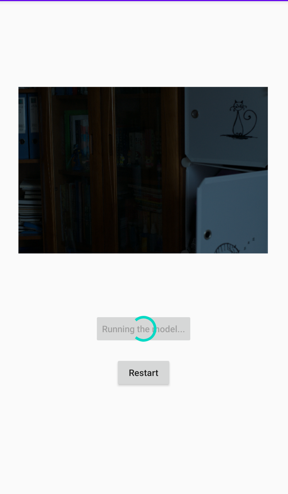

Mobile Implementation. We implement out method and create an application on Android system by Android Studio based on the repository of PyTorch on Android 222https://github.com/pytorch/android-demo-app/. As seen in Fig. 17, our model can achieve an accurate enhancement result on a type of mobile device, Huawei Mate 20. The runtime on the device is 0.439 second per frame. The experiment shows the feasibility of applying our lightweight model to mobile application. We also trial implementing several other lightweight methods on the mobile device and test their inference time. For NightEnhance (Jin et al., 2022) and PairLIE (Fu et al., 2023b), the buffer usage exceeds the device limit during converting datatype. The results are shown in Table 5. Note that the mobile implementation of PyTorch is on CPU.
| ZeroDCE | ZeroDCE++ | SCI | Ours | |
|---|---|---|---|---|
| runtime | 0.822 | 0.701 | 0.762 | 0.439 |
| PSNR | 14.86 | 15.34 | 14.78 | 21.54 |
6 Conclusion
In this work, we extend the classic Retinex theory, targeted initially at formulating scene radiance reaching human eyes, to a complex form taking noise, quantization error, non-linearity response function, and dynamic range limitation into consideration. By incorporating these factors, we demonstrate that the LLIE problem can be modeled through a pixel-wise linear restoration function that includes an offset with non-zero mean, which was previously ignored in other works. Besides we introduce a contrast brightness adjustment function for enhancing low-light images in a zero-shot learning manner. A masked reverse degradation loss in Gamma space and a variance suppression loss for regulating the offset feature are derived from the proposed LLIE model. The reverse degradation process darkens an enhanced image back to the input low-light image, thereby reducing the offset. Our method can achieve the best performance with the fewest parameters and the least runtime.
References
- Abdullah-Al-Wadud et al. [2007] M. Abdullah-Al-Wadud, M. H. Kabir, M. A. A. Dewan, and O. Chae. A dynamic histogram equalization for image contrast enhancement. IEEE Transactions on Consumer Electronics, 53(2):593–600, 2007.
- Alter et al. [2006] F. Alter, Y. Matsushita, and X. Tang. An intensity similarity measure in low-light conditions. In European Conference on Computer Vision, pages 267–280. Springer, 2006.
- [3] android gpuimage. Source code for gpuimagecontrastfilter. [EB/OL]. https://github.com/cats-oss/android-gpuimage/blob/master/library/src/main/java/jp/co/cyberagent/android/gpuimage/filter/.
- Antal et al. [2001] T. Antal, M. Droz, G. Györgyi, and Z. Rácz. 1/f noise and extreme value statistics. Physical review letters, 87(24):240601, 2001.
- [5] F. Banterle, A. Artusi, K. Debattista, and A. Chalmers. Advanced high dynamic range imaging: Theory and practice,(2011).
- Blanter and Büttiker [2000] Y. M. Blanter and M. Büttiker. Shot noise in mesoscopic conductors. Physics reports, 336(1-2):1–166, 2000.
- Cai et al. [2017] B. Cai, X. Xu, K. Guo, K. Jia, B. Hu, and D. Tao. A joint intrinsic-extrinsic prior model for retinex. In Proceedings of the IEEE international conference on computer vision, pages 4000–4009, 2017.
- Cai et al. [2018] J. Cai, S. Gu, and L. Zhang. Learning a deep single image contrast enhancer from multi-exposure images. IEEE Transactions on Image Processing, 27(4):2049–2062, 2018.
- Cai et al. [2023] Y. Cai, H. Bian, J. Lin, H. Wang, R. Timofte, and Y. Zhang. Retinexformer: One-stage retinex-based transformer for low-light image enhancement. In Proceedings of the IEEE/CVF International Conference on Computer Vision (ICCV), pages 12504–12513, October 2023.
- Chen et al. [2018] C. Chen, Q. Chen, J. Xu, and V. Koltun. Learning to see in the dark. In Proceedings of the IEEE conference on computer vision and pattern recognition, pages 3291–3300, 2018.
- Chen et al. [2019] C. Chen, Q. Chen, M. N. Do, and V. Koltun. Seeing motion in the dark. In Proceedings of the IEEE/CVF International Conference on Computer Vision, pages 3185–3194, 2019.
- Coltuc et al. [2006] D. Coltuc, P. Bolon, and J.-M. Chassery. Exact histogram specification. IEEE Transactions on Image processing, 15(5):1143–1152, 2006.
- Dong et al. [2010] X. Dong, Y. Pang, and J. Wen. Fast efficient algorithm for enhancement of low lighting video. In ACM SIGGRAPH 2010 Posters, pages 1–1. 2010.
- Fan et al. [2020] M. Fan, W. Wang, W. Yang, and J. Liu. Integrating semantic segmentation and retinex model for low-light image enhancement. In Proceedings of the 28th ACM international conference on multimedia, pages 2317–2325, 2020.
- [15] A. C. Fredrik Lundh and Contributors. Source code for pil.imageenhance. [EB/OL]. https://pillow.readthedocs.io/en/stable/_modules/PIL/ImageEnhance.html#Contrast.
- Fu et al. [2023a] H. Fu, W. Zheng, X. Meng, X. Wang, C. Wang, and H. Ma. You do not need additional priors or regularizers in retinex-based low-light image enhancement. In Proceedings of the IEEE/CVF Conference on Computer Vision and Pattern Recognition (CVPR), pages 18125–18134, June 2023a.
- Fu et al. [2018] Q. Fu, C. Jung, and K. Xu. Retinex-based perceptual contrast enhancement in images using luminance adaptation. IEEE Access, 6:61277–61286, 2018.
- Fu et al. [2014] X. Fu, Y. Sun, M. LiWang, Y. Huang, X.-P. Zhang, and X. Ding. A novel retinex based approach for image enhancement with illumination adjustment. In 2014 IEEE International Conference on Acoustics, Speech and Signal Processing (ICASSP), pages 1190–1194. IEEE, 2014.
- Fu et al. [2016a] X. Fu, D. Zeng, Y. Huang, Y. Liao, X. Ding, and J. Paisley. A fusion-based enhancing method for weakly illuminated images. Signal Processing, 129:82–96, 2016a.
- Fu et al. [2016b] X. Fu, D. Zeng, Y. Huang, X.-P. Zhang, and X. Ding. A weighted variational model for simultaneous reflectance and illumination estimation. In Proceedings of the IEEE conference on computer vision and pattern recognition, pages 2782–2790, 2016b.
- Fu et al. [2023b] Z. Fu, Y. Yang, X. Tu, Y. Huang, X. Ding, and K.-K. Ma. Learning a simple low-light image enhancer from paired low-light instances. In Proceedings of the IEEE/CVF Conference on Computer Vision and Pattern Recognition, pages 22252–22261, 2023b.
- Guo et al. [2020] C. Guo, C. Li, J. Guo, C. C. Loy, J. Hou, S. Kwong, and R. Cong. Zero-reference deep curve estimation for low-light image enhancement. In Proceedings of the IEEE/CVF Conference on Computer Vision and Pattern Recognition, pages 1780–1789, 2020.
- Guo et al. [2016] X. Guo, Y. Li, and H. Ling. Lime: Low-light image enhancement via illumination map estimation. IEEE Transactions on image processing, 26(2):982–993, 2016.
- Haus [2000] H. A. Haus. Electromagnetic noise and quantum optical measurements. Springer Science & Business Media, 2000.
- Healey and Kondepudy [1994] G. E. Healey and R. Kondepudy. Radiometric ccd camera calibration and noise estimation. IEEE Transactions on Pattern Analysis and Machine Intelligence, 16(3):267–276, 1994.
- Ibrahim and Kong [2007] H. Ibrahim and N. S. P. Kong. Brightness preserving dynamic histogram equalization for image contrast enhancement. IEEE Transactions on Consumer Electronics, 53(4):1752–1758, 2007.
- Janesick [2007] J. R. Janesick. Photon transfer. SPIE, 2007.
- Jiang and Zheng [2019] H. Jiang and Y. Zheng. Learning to see moving objects in the dark. In 2019 IEEE/CVF International Conference on Computer Vision (ICCV), pages 7323–7332, 2019. doi: 10.1109/ICCV.2019.00742.
- Jiang et al. [2021] Y. Jiang, X. Gong, D. Liu, Y. Cheng, C. Fang, X. Shen, J. Yang, P. Zhou, and Z. Wang. Enlightengan: Deep light enhancement without paired supervision. IEEE Transactions on Image Processing, 30:2340–2349, 2021.
- Jin et al. [2022] Y. Jin, W. Yang, and R. T. Tan. Unsupervised night image enhancement: When layer decomposition meets light-effects suppression. In European Conference on Computer Vision, pages 404–421. Springer, 2022.
- Jobson et al. [1997a] D. J. Jobson, Z.-u. Rahman, and G. A. Woodell. A multiscale retinex for bridging the gap between color images and the human observation of scenes. IEEE Transactions on Image processing, 6(7):965–976, 1997a.
- Jobson et al. [1997b] D. J. Jobson, Z.-u. Rahman, and G. A. Woodell. Properties and performance of a center/surround retinex. IEEE transactions on image processing, 6(3):451–462, 1997b.
- Land [1977] E. H. Land. The retinex theory of color vision. Scientific american, 237(6):108–129, 1977.
- Land and McCann [1971] E. H. Land and J. J. McCann. Lightness and retinex theory. Josa, 61(1):1–11, 1971.
- Lee et al. [2013a] C. Lee, C. Lee, and C.-S. Kim. Contrast enhancement based on layered difference representation of 2d histograms. IEEE transactions on image processing, 22(12):5372–5384, 2013a.
- Lee et al. [2013b] C.-H. Lee, J.-L. Shih, C.-C. Lien, and C.-C. Han. Adaptive multiscale retinex for image contrast enhancement. In 2013 International Conference on Signal-Image Technology & Internet-Based Systems, pages 43–50. IEEE, 2013b.
- Li et al. [2018a] C. Li, J. Guo, F. Porikli, and Y. Pang. Lightennet: A convolutional neural network for weakly illuminated image enhancement. Pattern recognition letters, 104:15–22, 2018a.
- Li et al. [2021a] C. Li, C. Guo, L.-H. Han, J. Jiang, M.-M. Cheng, J. Gu, and C. C. Loy. Low-light image and video enhancement using deep learning: A survey. IEEE Transactions on Pattern Analysis & Machine Intelligence, (01):1–1, 2021a.
- Li et al. [2021b] C. Li, C. G. Guo, and C. C. Loy. Learning to enhance low-light image via zero-reference deep curve estimation. In IEEE Transactions on Pattern Analysis and Machine Intelligence, 2021b. doi: 10.1109/TPAMI.2021.3063604.
- Li et al. [2019] J. Li, Y. Wang, C. Wang, Y. Tai, J. Qian, J. Yang, C. Wang, J. Li, and F. Huang. Dsfd: Dual shot face detector. In Proceedings of the IEEE Conference on Computer Vision and Pattern Recognition, 2019.
- Li et al. [2015] L. Li, R. Wang, W. Wang, and W. Gao. A low-light image enhancement method for both denoising and contrast enlarging. In 2015 IEEE international conference on image processing (ICIP), pages 3730–3734. IEEE, 2015.
- Li et al. [2018b] M. Li, J. Liu, W. Yang, X. Sun, and Z. Guo. Structure-revealing low-light image enhancement via robust retinex model. IEEE Transactions on Image Processing, 27(6):2828–2841, 2018b.
- Liu et al. [2021] R. Liu, L. Ma, J. Zhang, X. Fan, and Z. Luo. Retinex-inspired unrolling with cooperative prior architecture search for low-light image enhancement. In Proceedings of the IEEE/CVF Conference on Computer Vision and Pattern Recognition, pages 10561–10570, 2021.
- Liu et al. [2022] R. Liu, L. Ma, T. Ma, X. Fan, and Z. Luo. Learning with nested scene modeling and cooperative architecture search for low-light vision. IEEE Transactions on Pattern Analysis and Machine Intelligence, 45(5):5953–5969, 2022.
- Lore et al. [2017] K. G. Lore, A. Akintayo, and S. Sarkar. Llnet: A deep autoencoder approach to natural low-light image enhancement. Pattern Recognition, 61:650–662, 2017.
- Lv et al. [2018] F. Lv, F. Lu, J. Wu, and C. Lim. Mbllen: Low-light image/video enhancement using cnns. In BMVC, volume 220, page 4, 2018.
- Ma et al. [2022] L. Ma, T. Ma, R. Liu, X. Fan, and Z. Luo. Toward fast, flexible, and robust low-light image enhancement. In Proceedings of the IEEE/CVF Conference on Computer Vision and Pattern Recognition, pages 5637–5646, 2022.
- Mackay et al. [2001] C. D. Mackay, R. N. Tubbs, R. Bell, D. J. Burt, P. Jerram, and I. Moody. Subelectron read noise at mhz pixel rates. In Sensors and Camera Systems for Scientific, Industrial, and Digital Photography Applications II, volume 4306, pages 289–298. SPIE, 2001.
- Mann and Picard [1994] S. Mann and R. Picard. Beingundigital’with digital cameras. MIT Media Lab Perceptual, 1:2, 1994.
- Mertens et al. [2007] T. Mertens, J. Kautz, and F. Van Reeth. Exposure fusion. In 15th Pacific Conference on Computer Graphics and Applications (PG’07), pages 382–390. IEEE, 2007.
- Mertens et al. [2009] T. Mertens, J. Kautz, and F. Van Reeth. Exposure fusion: A simple and practical alternative to high dynamic range photography. In Computer graphics forum, volume 28, pages 161–171. Wiley Online Library, 2009.
- Mitsunaga and Nayar [1999] T. Mitsunaga and S. K. Nayar. Radiometric self calibration. In Proceedings. 1999 IEEE computer society conference on computer vision and pattern recognition (Cat. No PR00149), volume 1, pages 374–380. IEEE, 1999.
- Moon et al. [2007] C.-R. Moon, J. Jung, D.-W. Kwon, J. Yoo, D.-H. Lee, and K. Kim. Application of plasma-doping (plad) technique to reduce dark current of cmos image sensors. IEEE electron device letters, 28(2):114–116, 2007.
- Padmavathy and Priya [2018] V. Padmavathy and R. Priya. Image contrast enhancement techniques-a survey. International Journal of Engineering & Technology, 7(2.33):466–469, 2018.
- Park et al. [2018] S. Park, K. Kim, S. Yu, and J. Paik. Contrast enhancement for low-light image enhancement: A survey. IEIE Transactions on Smart Processing and Computing, 7:36–48, 2018.
- Paszke et al. [2019] A. Paszke, S. Gross, F. Massa, A. Lerer, J. Bradbury, G. Chanan, T. Killeen, Z. Lin, N. Gimelshein, L. Antiga, et al. Pytorch: An imperative style, high-performance deep learning library. Advances in neural information processing systems, 32, 2019.
- Pizer [1990] S. M. Pizer. Contrast-limited adaptive histogram equalization: Speed and effectiveness stephen m. pizer, r. eugene johnston, james p. ericksen, bonnie c. yankaskas, keith e. muller medical image display research group. In Proceedings of the first conference on visualization in biomedical computing, Atlanta, Georgia, volume 337, page 1, 1990.
- Ren et al. [2019] W. Ren, S. Liu, L. Ma, Q. Xu, X. Xu, X. Cao, J. Du, and M.-H. Yang. Low-light image enhancement via a deep hybrid network. IEEE Transactions on Image Processing, 28(9):4364–4375, 2019.
- Ren et al. [2018] X. Ren, M. Li, W.-H. Cheng, and J. Liu. Joint enhancement and denoising method via sequential decomposition. In 2018 IEEE international symposium on circuits and systems (ISCAS), pages 1–5. IEEE, 2018.
- Schottky [1918] W. Schottky. Über spontane stromschwankungen in verschiedenen elektrizitätsleitern. Annalen der physik, 362(23):541–567, 1918.
- Stark [2000] J. A. Stark. Adaptive image contrast enhancement using generalizations of histogram equalization. IEEE Transactions on image processing, 9(5):889–896, 2000.
- Vijayalakshmi et al. [2020] D. Vijayalakshmi, M. K. Nath, and O. P. Acharya. A comprehensive survey on image contrast enhancement techniques in spatial domain. Sensing and Imaging, 21(1):1–40, 2020.
- Wang et al. [2014] L. Wang, L. Xiao, H. Liu, and Z. Wei. Variational bayesian method for retinex. IEEE Transactions on Image Processing, 23(8):3381–3396, 2014.
- Wang et al. [2020] L.-W. Wang, Z.-S. Liu, W.-C. Siu, and D. P. Lun. Lightening network for low-light image enhancement. IEEE Transactions on Image Processing, 29:7984–7996, 2020.
- Wang et al. [2019a] R. Wang, Q. Zhang, C.-W. Fu, X. Shen, W.-S. Zheng, and J. Jia. Underexposed photo enhancement using deep illumination estimation. In Proceedings of the IEEE/CVF Conference on Computer Vision and Pattern Recognition, pages 6849–6857, 2019a.
- Wang et al. [2013] S. Wang, J. Zheng, H.-M. Hu, and B. Li. Naturalness preserved enhancement algorithm for non-uniform illumination images. IEEE transactions on image processing, 22(9):3538–3548, 2013.
- Wang et al. [2019b] Y. Wang, Y. Cao, Z.-J. Zha, J. Zhang, Z. Xiong, W. Zhang, and F. Wu. Progressive retinex: Mutually reinforced illumination-noise perception network for low-light image enhancement. In Proceedings of the 27th ACM international conference on multimedia, pages 2015–2023, 2019b.
- Wang et al. [2022] Y. Wang, R. Wan, W. Yang, H. Li, L.-P. Chau, and A. Kot. Low-light image enhancement with normalizing flow. In Proceedings of the AAAI Conference on Artificial Intelligence, volume 36, pages 2604–2612, 2022.
- Wang et al. [2023a] Y. Wang, Z. Liu, J. Liu, S. Xu, and S. Liu. Low-light image enhancement with illumination-aware gamma correction and complete image modelling network. In Proceedings of the IEEE/CVF International Conference on Computer Vision (ICCV), pages 13128–13137, October 2023a.
- Wang et al. [2023b] Y. Wang, Y. Yu, W. Yang, L. Guo, L.-P. Chau, A. C. Kot, and B. Wen. Exposurediffusion: Learning to expose for low-light image enhancement. In Proceedings of the IEEE/CVF International Conference on Computer Vision (ICCV), pages 12438–12448, October 2023b.
- Wang et al. [2004] Z. Wang, A. C. Bovik, H. R. Sheikh, and E. P. Simoncelli. Image quality assessment: from error visibility to structural similarity. IEEE transactions on image processing, 13(4):600–612, 2004.
- Weber [1831] E. H. Weber. De Pulsu, resorptione, auditu et tactu: Annotationes anatomicae et physiologicae… CF Koehler, 1831.
- Wei et al. [2018] C. Wei, W. Wang, W. Yang, and J. Liu. Deep retinex decomposition for low-light enhancement. In British Machine Vision Conference, 2018.
- Wu et al. [2022] W. Wu, J. Weng, P. Zhang, X. Wang, W. Yang, and J. Jiang. Uretinex-net: Retinex-based deep unfolding network for low-light image enhancement. In Proceedings of the IEEE/CVF Conference on Computer Vision and Pattern Recognition, pages 5901–5910, 2022.
- Wu et al. [2023] Y. Wu, C. Pan, G. Wang, Y. Yang, J. Wei, C. Li, and H. T. Shen. Learning semantic-aware knowledge guidance for low-light image enhancement. In Proceedings of the IEEE/CVF Conference on Computer Vision and Pattern Recognition (CVPR), pages 1662–1671, June 2023.
- Xu et al. [2020a] J. Xu, Y. Hou, D. Ren, L. Liu, F. Zhu, M. Yu, H. Wang, and L. Shao. Star: A structure and texture aware retinex model. IEEE Transactions on Image Processing, 29:5022–5037, 2020a.
- Xu et al. [2020b] K. Xu, X. Yang, B. Yin, and R. W. Lau. Learning to restore low-light images via decomposition-and-enhancement. In Proceedings of the IEEE/CVF Conference on Computer Vision and Pattern Recognition, pages 2281–2290, 2020b.
- Xu et al. [2022] X. Xu, R. Wang, C.-W. Fu, and J. Jia. Snr-aware low-light image enhancement. In Proceedings of the IEEE/CVF Conference on Computer Vision and Pattern Recognition, pages 17714–17724, 2022.
- Xu et al. [2023] X. Xu, R. Wang, and J. Lu. Low-light image enhancement via structure modeling and guidance. In Proceedings of the IEEE/CVF Conference on Computer Vision and Pattern Recognition (CVPR), pages 9893–9903, June 2023.
- Yang et al. [2016] S. Yang, P. Luo, C.-C. Loy, and X. Tang. Wider face: A face detection benchmark. In Proceedings of the IEEE conference on computer vision and pattern recognition, pages 5525–5533, 2016.
- Yang et al. [2020] W. Yang, S. Wang, Y. Fang, Y. Wang, and J. Liu. From fidelity to perceptual quality: A semi-supervised approach for low-light image enhancement. In Proceedings of the IEEE/CVF conference on computer vision and pattern recognition, pages 3063–3072, 2020.
- Yang et al. [2021a] W. Yang, S. Wang, Y. Fang, Y. Wang, and J. Liu. Band representation-based semi-supervised low-light image enhancement: Bridging the gap between signal fidelity and perceptual quality. IEEE Transactions on Image Processing, 30:3461–3473, 2021a.
- Yang et al. [2021b] W. Yang, W. Wang, H. Huang, S. Wang, and J. Liu. Sparse gradient regularized deep retinex network for robust low-light image enhancement. IEEE Transactions on Image Processing, 30:2072–2086, 2021b.
- Yi et al. [2023] X. Yi, H. Xu, H. Zhang, L. Tang, and J. Ma. Diff-retinex: Rethinking low-light image enhancement with a generative diffusion model. In Proceedings of the IEEE/CVF International Conference on Computer Vision (ICCV), pages 12302–12311, October 2023.
- Ying et al. [2017] Z. Ying, G. Li, Y. Ren, R. Wang, and W. Wang. A new low-light image enhancement algorithm using camera response model. In Proceedings of the IEEE International Conference on Computer Vision Workshops, pages 3015–3022, 2017.
- Yuan and Sun [2012] L. Yuan and J. Sun. Automatic exposure correction of consumer photographs. In European Conference on Computer Vision, pages 771–785. Springer, 2012.
- Yuan et al. [2019] Y. Yuan, W. Yang, W. Ren, J. Liu, W. J. Scheirer, and Z. Wang. Ug 2+ track 2: A collective benchmark effort for evaluating and advancing image understanding in poor visibility environments. arXiv preprint arXiv:1904.04474, 2019.
- Zhang et al. [2021] F. Zhang, Y. Li, S. You, and Y. Fu. Learning temporal consistency for low light video enhancement from single images. In Proceedings of the IEEE/CVF Conference on Computer Vision and Pattern Recognition, pages 4967–4976, 2021.
- Zhang et al. [2019a] L. Zhang, L. Zhang, X. Liu, Y. Shen, S. Zhang, and S. Zhao. Zero-shot restoration of back-lit images using deep internal learning. In Proceedings of the 27th ACM International Conference on Multimedia, pages 1623–1631, 2019a.
- Zhang et al. [2018] R. Zhang, P. Isola, A. A. Efros, E. Shechtman, and O. Wang. The unreasonable effectiveness of deep features as a perceptual metric. In Proceedings of the IEEE conference on computer vision and pattern recognition, pages 586–595, 2018.
- Zhang et al. [2019b] Y. Zhang, J. Zhang, and X. Guo. Kindling the darkness: A practical low-light image enhancer. In Proceedings of the 27th ACM international conference on multimedia, pages 1632–1640, 2019b.
- Zhang et al. [2022] Z. Zhang, H. Zheng, R. Hong, M. Xu, S. Yan, and M. Wang. Deep color consistent network for low-light image enhancement. In Proceedings of the IEEE/CVF Conference on Computer Vision and Pattern Recognition, pages 1899–1908, 2022.
- Zhao et al. [2021] Z. Zhao, B. Xiong, L. Wang, Q. Ou, L. Yu, and F. Kuang. Retinexdip: A unified deep framework for low-light image enhancement. IEEE Transactions on Circuits and Systems for Video Technology, 32(3):1076–1088, 2021.
- Zhu et al. [2020a] A. Zhu, L. Zhang, Y. Shen, Y. Ma, S. Zhao, and Y. Zhou. Zero-shot restoration of underexposed images via robust retinex decomposition. In 2020 IEEE International Conference on Multimedia and Expo (ICME), pages 1–6. IEEE, 2020a.
- Zhu et al. [2020b] M. Zhu, P. Pan, W. Chen, and Y. Yang. Eemefn: Low-light image enhancement via edge-enhanced multi-exposure fusion network. In Proceedings of the AAAI Conference on Artificial Intelligence, volume 34, pages 13106–13113, 2020b.
Appendix
Notation
We first briefly summarise the notations in the paper.
6.1 Derivation of Eq. 10
We have the expressions of DI-Retinex theory for both low light and normally exposed images as follows:
Plug the expression of .
By transforming the first expression, we have
Plug it into the expression of extended Retinex theory for normally exposed image. Suppose . Then we have
According to the approximation that
| (25) |
when by Taylor expansion, we can get
Note that , and thus . The noise term is small. When , we have and , which ensures compared to the maximum intensity of for . When at -th pixel, also equals zero and thus . Besides, the probability of exactly equaling to zero is extremely small among pixels in reality. The second term is thus much smaller than the other terms and can be safely omitted, which yields
Therefore, we can obtain
| where |
6.2 Derivation of Eq. 18
We want to show
| where |
Similar to the derivation of Eq. 10, we start from
and we can get
Then by using approximation in Eq. 25 we have
Let the second term be
Note that , and thus . The noise term is small. When , we have and , which ensures compared to the maximum intensity. When at -th pixel, also equals zero and thus . Besides, the probability of exactly equaling to zero is extremely small among pixels in reality. The second term is thus much smaller than the other terms and can be safely omitted, which yields
Therefore, we can obtain
| where |
6.3 Discussion of Linear Model and the Offset
The expression of is given by
where . We analyse the magnitude of by computing its mean and variance. Given and and suppose is independent of and , we have
A properly exposed has equal probability of overexposure and underexposure. Thus . Also a negative overflow exceeding caused by a negative image irradiance is seldom and thus . is a negative number such that the Gamma transformation can map to . (found in the following statistical experiments) makes the magnitude of significant. Even if in some rare case, has non-zero values only in some regions of an image and has large values in the regions where has zero values. Therefore, is not negligible in terms of considerable mean.
We then compute ’s variance. The variance of is zero as it is a constant. Since the quantization error follows a uniform distribution from to , its variance is . Note that with the assumption of flux consistency along time dimension across spatial pixels during receiving radiance in a short period, can be further treated as a constant matrix. So it can be considered as a scalar when computing ’s variance,
As shown, the factor of enlarges the variance of . The amplified variance also makes non-negligible.
6.4 Discussion on Reverse Degradation
The expression of is given by
where . We analyse the magnitude of by computing its mean and variance. Given and and suppose is independent of and , we have
A properly exposed has equal probability of overexposure and underexposure. Thus . Also a negative overflow exceeding caused by a negative image irradiance is seldom and thus . is a negative number such that the Gamma transformation can map to . . This makes getting small. For even more safely removing , we compute reverse degradation loss in Gamma space by taking a power of , which suppresses the magnitude of .
We then compute the variance of . Similar to Section 6.3, we can get
where represents the scalar form of , assuming flux consistency across spatial pixels over a brief time period when receiving radiance. As depicted, the factor assumes a small value, given that is less than 1 while the max pixel value is 255. The variance of closely approximates , which denotes the variance arising from error and offset terms in low-light images. It is important to note that the variance is small and thus approaching zero.
6.5 Discussion on Mapping Function and Contrast Brightness Algorithm
We use four nonlinear function mapping to . According to the finding of statistical experiments in Section 6.3. The ratio between the exposures of low light and normally exposed images is mainly within , we thus make sure that most output values of mapping function lie in the region. The formula of four used functions are given below and their curves are drawn in Fig. 18.
A shifted reciprocal function like is a straightforward and common choice. But we can see that has an extremely steep rise when and thus generates the worst result in Table. 4. To alleviate the steep rise, we apply a logarithm function to shifted and form . It coincidentally becomes a shifted inverse hyperbolic tangent function. But it still cannot lead to a good enough performance. Then we choose a tangent function and its performance is satisfactory. We further try its logarithm with a gentler slope. It has even better effect but the nesting of two nonlinear functions yields more computations. Considering the trade-off, we just use .
The majority of existing works about image contrast enhancement are based on histogram equalization [Padmavathy and Priya, 2018, Vijayalakshmi et al., 2020, Park et al., 2018]. Though some variants of Eq. 17 is used empirically in industry for adjusting image’s contrast, there is no academic paper discussing it to the best of our knowledge. One of our contributions lies in employing it to solve low light enhancement problem with the zero-reference regulation of two losses. Compared with other functions with single coefficient, the formula involving two coefficients is more difficult for a neural network to learn. Our derived reverse degradation loss and variance suppression loss can effectively guide the network to learn the coefficient pair of the adjustment function. We experiment various mapping functions aforementioned and modified the original formulation with the best choice of .
6.6 Network Structure
Our model is extremely simple and its structure is shown in Table 6.
| layer | channel_in | channel_out | kernel | stride | padding |
|---|---|---|---|---|---|
| Conv+ReLU | 3 | 3 | 1 | 1 | |
| Conv+ReLU | 3 | 1 | 1 | ||
| Conv+Tanh | 3 | 1 | 1 |
6.7 Decomposition Visualization
We showcase an visual example of decomposition of our enhancement model in Fig. 19.