Constraints on the Cosmic Neutrino Background from NGC 1068
Abstract
We use recent evidence of TeV neutrino events from NGC 1068, detected by the IceCube experiment, to constrain the overdensity of relic neutrinos locally and globally. Since these high-energy neutrinos have travelled long distances through a sea of relic neutrinos, they could have undergone scattering, altering their observed flux on Earth. Considering only Standard Model interactions, we constrain the relic overdensity to be at the 95 confidence level for overdensities with a radius of 14 Mpc (10 kpc), assuming the sum of neutrino masses saturates the cosmological bound, eV. We demonstrate that this limit improves with larger neutrino masses and how it depends on the scale of the overdensity region.
The CDM standard cosmology model predicts a neutrino background akin to the observed cosmic microwave background. The discovery of such relic neutrinos would mark a significant breakthrough for cosmology and particle physics, offering a path to unveil fundamental neutrino properties such as their masses and whether they are Dirac or Majorana particles Long et al. (2014). However, detecting these relic neutrinos experimentally has proven to be remarkably challenging. This is primarily because these neutrinos have low momenta, approximately eV, resulting in only a few possible interaction channels to detect these neutrinos. Nonetheless, there are numerous proposals for relic neutrino detection including capture on radioactive nuclei Weinberg (1962); Baracchini et al. (2018), observing the annihilation of ultra-high energy cosmic ray neutrinos with the relic neutrino background using the -resonance Eberle et al. (2004), elastic scattering of the relic neutrino wind on a test mass Stodolsky (1975); Opher (1974); Duda et al. (2001); Domcke and Spinrath (2017); Shvartsman et al. (1982); Smith and Lewin (1983); Cabibbo and Maiani (1982), looking for alterations in atomic deexcitation spectra Yoshimura et al. (2015) and resonant neutrino capture in accelerator experiments Bauer and Shergold (2021).
These ideas, which may become experimentally feasible in the future, are hindered by anticipated minuscule rates of detected neutrinos; see Ref. Bauer and Shergold (2023a) for a comprehensive overview of experimental sensitivities. This necessitates either large quantities of detector material or the experimental detection of extremely subtle effects, rendering detection exceptionally challenging. However, there is a caveat that could potentially alter the anticipated rates in a future facility: while the CDM model predicts a neutrino density of approximately for each mass state (and similarly for antineutrinos) Giunti and Kim (2007), there could be an enhancement of the neutrino number density due to gravitational clustering. Such an overdensity seems to be above the average predicted by the CDM model. Nonetheless, it could be much larger depending on whether there are additional beyond-the-Standard Model (BSM) interactions impacting neutrinos Ringwald and Wong (2004); de Salas et al. (2017); Holm et al. (2023); Zimmer et al. (2023); Elbers et al. (2023); Elbers (2023). Thus, it may be prudent to first experimentally constrain potential overdensities before attempting a direct detection of the Cosmic Neutrino Background (CB).
Constraints on overdensities stem from both theoretical and experimental sides. On the one hand, clustering large amounts of neutrinos would be prohibited by the Pauli exclusion principle Tremaine and Gunn (1979); Bauer and Shergold (2021). Since the standard CB is expected to be close to the Pauli limit, any large overdensity would indicate not only the presence of additional interactions, but also that the relic neutrinos would possess a larger temperature to the one expected in standard cosmology. On the other hand, the KATRIN experiment recently has managed to constrain the local overdensity through a direct search for events consistent with the detection of the CB, resulting in a limit of times the average density predicted by cosmology Aker et al. (2022). Another possible way to constrain relic neutrino overdensities consists in determining the effects from scattering of high energy particles with the CB, such as detecting CB neutrinos boosted by the Diffuse Supernova Neutrino Background Das et al. (2022), cosmic rays Císcar-Monsalvatje et al. (2024), detecting absorption features in the cosmogenic neutrinos spectrum Brdar et al. (2022), or considering the gravitational effect on Solar System objects Tsai et al. (2024).
A recent analysis of the high-energy events detected by IceCube has unveiled the origins of some of these astrophysical neutrinos. The most significant among the candidate sources is the active galaxy NGC 1068 Abbasi et al. (2022); Aartsen et al. (2020), with a global significance of . The discovery of these neutrino point sources presents an opportunity for studying scenarios Beyond the Standard Model by exploring deviations in the expected neutrino flux from the source, see e.g. Ng and Beacom (2014); Esteban et al. (2021); Carloni et al. (2022); Rink and Sen (2024); Cline and Puel (2023); Döring and Vogl (2023). Crucially, these high-energy neutrinos traverse extensive distances through the CB on their way to Earth. Overdensities of these relic neutrinos, which lie along the path traversed by the astrophysical neutrinos, can potentially modify the astrophysical neutrino fluxes through the self-interactions of neutrinos, even within the Standard Model (SM). In this Letter, we seek to constrain the overabundance of relic neutrinos by analysing neutrino events from NGC 1068 using publicly available data from IceCube.
Relic Overdensity — Any deviation from the expected average number density of relic neutrinos, , can be parameterised by , where is the true number density. Local relic overdensities are predicted by standard CDM cosmology since neutrinos will cluster due to gravitational effects de Salas et al. (2017); Holm et al. (2023). However, these effects are predicted to be small, with ranging between 1.2 and 20 Aker et al. (2022). On the other hand, it is possible that some exotic scenarios could modify this significantly, producing larger overabundances over different scales Ringwald and Wong (2004); Tsai et al. (2024); Smirnov and Xu (2022); Fardon et al. (2004); Dvali and Funcke (2016). If there is a significant overabundance of relic neutrinos, interactions between relic and astrophysical neutrinos could impact the neutrino flux from NGC 1068 observed at IceCube.
To take into account the effect of scattering with relic neutrinos of the flux propagating to the Earth, it is necessary to solve a transport equation for the flux of neutrinos with mass state ,
| (1) |
where denotes the combined flux of neutrinos and anti-neutrinos with mass state , is the distance that the neutrinos have travelled from NGC 1068, is the number density of mass states and is the neutrino-neutrino cross-section. In the second term of Eq. (11), the state is the incoming neutrino with energy , the state is the relic neutrino, is the outgoing neutrino with the mass state of interest, and is the other neutrino state produced in the interaction. The first term of Eq. (11) accounts for the decrease in neutrino flux caused by scattering off of the CB, while the second term accounts for both down-scattering (energy loss of the neutrinos) and up-scattering of the relic neutrino. The centre-of-mass energy of the interaction of the astrophysical neutrino, with energy , with the relic neutrino of mass , assumed to be at rest111Note that large overdensities due to some BSM interactions might also imply that the relic neutrinos could be relativistic today, enhancing the center-of-mass energy. However, we refrain from considering such a scenario to keep our discussion as model-independent as possible., is
| (2) |
and is always sufficiently small that the only important processes are , , and .
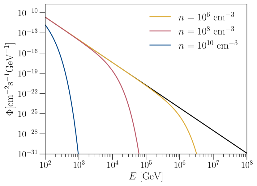
For the neutrinos originating from NGC 1068, we assume an initial power-law (PL) flux, where the flux is parameterised in terms of a normalisation , at a reference energy , and a spectral index such that ; throughout this Letter we take TeV. We also assume that the neutrino flavours are produced with the initial ratio of 1:2:0 for ::, which corresponds to pion decays Abdullahi and Denton (2020). To find the final flux at Earth, we solve the transport equation numerically over the distance that the neutrinos travel through the overdense region, . For a density that varies in value over spatial coordinates, for example, with gravitational clustering de Salas et al. (2017), is the radius of a constant density profile that would produce the same number of interactions. The effect of neutrino self-interactions over the astrophysical neutrino flux can be seen in Fig. 1, where the initial flux is plotted alongside the final flux for several different relic neutrino densities. The main effect is a suppression of the flux at high energies. Regeneration processes lead to an increased flux at lower energies; however, the influence at lower energies remains minimal due to the rapid decrease of the flux with energy.
Standard neutrino self-interactions — For the sake of simplicity, we limit our discussion to SM neutrino interactions and assume that the number density is the same for all mass states and for neutrinos/antineutrinos. We require both total and differential SM cross-sections to solve the transport equations in Eq. (11), which we will briefly outline next.
The total cross-section for the SM interactions between the neutrino flux from NGC 1068 and relic neutrinos can be split into two contributions: one from the production of neutrino final states only and one from the production of electron-positron pairs:
| (3) |
where is the incoming neutrino mass state, and is the relic neutrino mass state, as before. From this, we find that
| (4) |
where is the Fermi constant. This cross-section has been summed over the contributions from relic neutrinos and antineutrinos. For the cross-section with final states, the interaction must be calculated in the mass basis, such that
| (5) |
where is the flavour of the initial state neutrinos in the interaction. The production of only occurs with neutrino-antineutrino annihilation, so we can consider the initial flavours to be identical. The total cross-sections for this process are
| (6a) | ||||
| (6b) | ||||
where , with the weak mixing angle, the electron mass, and the Heaviside step function. Unlike in the case of the total cross-sections, when calculating the differential cross-section in the second term on the RHS of Eq. (11), we are interested in the kinematics of the final state of the interaction. In particular, we wish to obtain the differential cross-section in terms of the energy of the outgoing mass state (anti)neutrino. We find that the differential cross-section for neutrino pair production, taking all processes into account, is
| (7) |
where we have defined
| (8a) | ||||
| (8b) | ||||
We provide details of this calculation in the Supplementary Material for the interested reader.
Analysis — To search for CB overdensities within the IceCube data, we perform a maximum likelihood test Braun et al. (2008); Abbasi et al. (2022). The likelihood function for events, given a neutrino overdensity , is given by
| (9) |
where are the observables of the event , is the number of events associated with the signal, and and are the signal and background probability distribution functions (pdf), respectively. When performing the analysis, we consider the events from 2012-2018 taken from the public release IceCube Collaboration (2021), and select those within a 15∘ radius of NGC 1068.
We compare the hypothesis of a neutrino overdensity with the standard scenario by taking the log of the likelihood ratios
| (10) |
for each value of the neutrino overdensity, we minimise the test statistic () by marginalising over and . The likelihood of the null hypothesis () corresponds to the scenario where the CB density follows the prediction of the CDM model and the neutrino flux originated from NGC 1068 is described by and . These values are obtained through a analysis comparing the likelihoods between the power-law model and the scenario where all the data corresponds to the background.
The signal and background pdfs depend on the observables IceCube uses to reconstruct the astrophysical events. These include the reconstructed energy () and direction (), which can be decomposed into declination () and right ascension (), along with their uncertainties (). As the predominant backgrounds are atmospheric and diffuse astrophysical neutrinos, the background pdf is independent of the right ascension. We can thus construct the background pdf as
| (11) |
We neglect the dependence of on as it will be approximately equal to the dependence of on , and thus will cancel in the as can be seen in Eq. (10) Abbasi et al. (2022). To estimate the background pdf, we use a data scrambling method where we calculate the pdf of all events in the public data release IceCube Collaboration (2021) that were detected with declination in a window of 15∘ above and below NGC 1068 Aartsen et al. (2017). Doing so effectively integrates over right ascension. Since the number of background events far outweighs the number of signal events, this will approximate the true pdf of the background events well Aartsen et al. (2017).
The signal pdf can be decomposed into the product of the directional and the energy pdfs Abbasi et al. (2022)
| (12) |
where is the declination of the assumed source and are the model parameters. For a PL flux, there is only one relevant parameter, , whereas for the CB scattered flux, there are two parameters . We approximate the directional pdf, , as a Rayleigh distribution, as was done in Braun et al. (2008). This can be improved by using better models of the detector response, for example, considering the effect of energy on the spatial reconstruction Abbasi et al. (2022). The energy pdf in Eq. (12) is calculated from the following integral Bellenghi et al. (2023)
| (13) |
where is the pdf of reconstructed muon energies given an initial neutrino energy coming from a source with declination . This is taken from the detector response functions. The neutrino energy pdf, , is calculated from the flux and effective area. The detector response functions and the effective area are taken from the public release from IceCube IceCube Collaboration (2021).
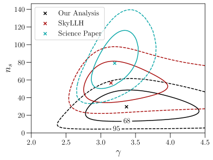
Applying the maximum likelihood method outlined above, we utilised IceCube data to assess the significance of the NGC 1068 source against a background-only hypothesis to ensure the validity of our code, and we found a good agreement with the official results. Details regarding the comparison of the NGC 1068 source parameters obtained through our code with the IceCube official results in Ref. Abbasi et al. (2022) can be found in the Supplementary Material.
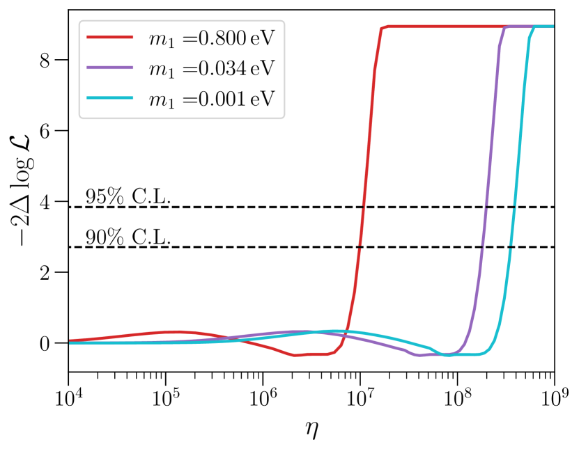
Results — In Fig. 2, we show the test statistic as a function of the CB overabundance parameter . Since the SM cross-sections are proportional to the centre-of-mass energy , and because we assume the relic neutrinos to be at rest, the values of that are probed will depend on the neutrino masses. As the absolute scale of the neutrino masses is not known, this analysis was repeated with different assumptions on the mass of the lightest neutrino, assuming normal ordering (NO) and using the mixing best-fit parameters from the NuFit global analysis Esteban et al. (2020).
We consider three scenarios for the value of the lightest neutrino mass. First, we employ the constraints on the sum of the neutrino masses coming from cosmological measurements, i.e. eV Abbott et al. (2022), and the best-fit values of the mass splittings from neutrino oscillation experiments to obtain a mass for the lightest neutrino of eV. Direct searches for neutrino masses, such as the one carried away by KATRIN experiment, set bound on the effective electron neutrino mass of The KATRIN Collaboration (2022), which is then translated to the value of the lightest neutrino mass of eV. Finally, we also consider a case where the lightest neutrino mass is small, but is still non-relativistic today, i.e. eV.
The strongest constraints on come from the larger values of , resulting from the increased centre-of-mass energy of the scattering processes, which leads to stronger interactions between the neutrinos. As seen in Fig. 2, there are some values of where the test statistic is negative, indicating a potential preference for this value. However, the value is small () and so well below being statistically significant. From further inspection of the contributions to the test statistic from each event, we find that the reduced statistics of higher energy muon events allow for this preference. The limiting factor on the strength of the constraint, i.e. the plateau observed at higher values of , is due to the limited strength of our analysis of NGC 1068 as a point source. At these values, the signal pdf of the scattered neutrino model goes to zero for all events as no signal events are predicted to be detected; this, in turn, means that the model likelihood tends towards a pure background. To push the exclusion bounds to higher confidence levels, we would require a larger likelihood value for the PL point-source analysis of NGC 1068.
Extending this analysis to a range of values of gives the results shown in Fig. 3, where the 90 and 95 C.L. are plotted for different effective distances of the overabundance. A value of Mpc implies that the relic density overabundance exists between Earth and NGC 1068, which could be the case if either there is some overdensity due to clustering on large scales. Also shown are the bounds for more conservative effective distances, corresponding to a local overdensity in the Milky Way or possibly in NGC 1068. We compare the bounds from this analysis to those produced by the KATRIN collaboration in Aker et al. (2022), which limit to less than for Dirac neutrinos at the 90 C.L. Unlike the KATRIN bounds, our constraints improve as increases due to the increase in the centre-of-mass energy. On the other hand, for small , the mass squared differences dominate in setting the mass scale, which results in an asymptotic limit.
It is also possible that other BSM scenarios could be constrained using a similar analysis. We performed a log-likelihood analysis on neutrino decays arising from a coupling to a massless Majoron. However, we found that current public data cannot constrain this scenario to a statistically significant degree as for all values of the coupling. This may change with improved reconstruction and more data Valera et al. (2023).
Final Thoughts — While there is a long way to go before experiments can begin to probe overdensities close to the Pauli exclusion limit, which is for a global overdensity Bauer and Shergold (2023b), the results from this analysis offer a significant improvement on the direct probing of the CB without any assumption of BSM physics. For any overabundance that spans between NGC 1068 and the Milky Way, this analysis places a bounds on that reaches () at the 90 (95) CL. These bounds will improve as more data from astrophysical sources are gathered. For example, the most recent result from NGC 1068 Abbasi et al. (2022), where the number of signal events has increased to , will enhance the exclusion overdensity to nearly . Additionally, as highlighted in Carloni et al. (2022); Blanco et al. (2023), other possible point sources could be added to this dataset, thereby enhancing the potential to constrain the relic neutrino density further. This outcome is expected to strengthen with upcoming experiments, such as IceCube Gen2 Aartsen et al. (2021), which is projected to increase the statistics by a factor of eight. Additionally, background reconstruction improvements will increase the significance of the limit on the neutrino overdensities.
.1 Acknowledgements
Acknowledgements.
We want to thank Jack Shergold for useful discussions and Carlos A. Argüelles and Martin Bauer for reading the draft version of this paper and for their helpful comments. The UK Science and Technology Facilities Council (STFC) has funded this work under grant ST/T001011/1. This project has received funding/support from the European Union’s Horizon 2020 research and innovation programme under the Marie Skłodowska-Curie grant agreement No 860881-HIDDeN. This work has made use of the Hamilton HPC Service of Durham University. This work used the DiRAC@Durham facility managed by the Institute for Computational Cosmology on behalf of the STFC DiRAC HPC Facility (www.dirac.ac.uk), which is part of the National eInfrastructure and funded by BEIS capital funding via STFC capital grants ST/P002293/1, ST/R002371/1 and ST/S002502/1, Durham University and STFC operations grant ST/R000832/1.References
- Long et al. (2014) A. J. Long, C. Lunardini, and E. Sabancilar, JCAP 08, 038 (2014), arXiv:1405.7654 [hep-ph] .
- Weinberg (1962) S. Weinberg, Phys. Rev. 128, 1457 (1962).
- Baracchini et al. (2018) E. Baracchini et al. (PTOLEMY), (2018), arXiv:1808.01892 [physics.ins-det] .
- Eberle et al. (2004) B. Eberle, A. Ringwald, L. Song, and T. J. Weiler, Phys. Rev. D 70, 023007 (2004), arXiv:hep-ph/0401203 .
- Stodolsky (1975) L. Stodolsky, Phys. Rev. Lett. 34, 110 (1975), [Erratum: Phys.Rev.Lett. 34, 508 (1975)].
- Opher (1974) R. Opher, Astron. Astrophys. 37, 135 (1974).
- Duda et al. (2001) G. Duda, G. Gelmini, and S. Nussinov, Phys. Rev. D 64, 122001 (2001), arXiv:hep-ph/0107027 .
- Domcke and Spinrath (2017) V. Domcke and M. Spinrath, JCAP 06, 055 (2017), arXiv:1703.08629 [astro-ph.CO] .
- Shvartsman et al. (1982) B. F. Shvartsman, V. B. Braginsky, S. S. Gershtein, Y. B. Zeldovich, and M. Y. Khlopov, JETP Lett. 36, 277 (1982).
- Smith and Lewin (1983) P. F. Smith and J. D. Lewin, Phys. Lett. B 127, 185 (1983).
- Cabibbo and Maiani (1982) N. Cabibbo and L. Maiani, Phys. Lett. B 114, 115 (1982).
- Yoshimura et al. (2015) M. Yoshimura, N. Sasao, and M. Tanaka, Phys. Rev. D 91, 063516 (2015), arXiv:1409.3648 [hep-ph] .
- Bauer and Shergold (2021) M. Bauer and J. D. Shergold, Phys. Rev. D 104, 083039 (2021), arXiv:2104.12784 [hep-ph] .
- Bauer and Shergold (2023a) M. Bauer and J. D. Shergold, JCAP 01, 003 (2023a), arXiv:2207.12413 [hep-ph] .
- Giunti and Kim (2007) C. Giunti and C. W. Kim, Fundamentals of Neutrino Physics and Astrophysics (2007).
- Ringwald and Wong (2004) A. Ringwald and Y. Y. Y. Wong, JCAP 12, 005 (2004), arXiv:hep-ph/0408241 .
- de Salas et al. (2017) P. F. de Salas, S. Gariazzo, J. Lesgourgues, and S. Pastor, JCAP 09, 034 (2017), arXiv:1706.09850 [astro-ph.CO] .
- Holm et al. (2023) E. B. Holm, I. M. Oldengott, and S. Zentarra, Phys. Lett. B 844, 138073 (2023), arXiv:2305.13379 [hep-ph] .
- Zimmer et al. (2023) F. Zimmer, C. A. Correa, and S. Ando, JCAP 11, 038 (2023), arXiv:2306.16444 [astro-ph.CO] .
- Elbers et al. (2023) W. Elbers, C. S. Frenk, A. Jenkins, B. Li, S. Pascoli, J. Jasche, G. Lavaux, and V. Springel, JCAP 10, 010 (2023), arXiv:2307.03191 [astro-ph.CO] .
- Elbers (2023) W. H. Elbers, Neutrinos from horizon to sub-galactic scales, Ph.D. thesis, Durham U. (2023).
- Tremaine and Gunn (1979) S. Tremaine and J. E. Gunn, Phys. Rev. Lett. 42, 407 (1979).
- Aker et al. (2022) M. Aker et al. (KATRIN), Phys. Rev. Lett. 129, 011806 (2022), arXiv:2202.04587 [nucl-ex] .
- Das et al. (2022) A. Das, Y. F. Perez-Gonzalez, and M. Sen, Phys. Rev. D 106, 095042 (2022), arXiv:2204.11885 [hep-ph] .
- Císcar-Monsalvatje et al. (2024) M. Císcar-Monsalvatje, G. Herrera, and I. M. Shoemaker, (2024), arXiv:2402.00985 [hep-ph] .
- Brdar et al. (2022) V. Brdar, P. S. B. Dev, R. Plestid, and A. Soni, Phys. Lett. B 833, 137358 (2022), arXiv:2207.02860 [hep-ph] .
- Tsai et al. (2024) Y.-D. Tsai, J. Eby, J. Arakawa, D. Farnocchia, and M. S. Safronova, JCAP 02, 029 (2024), arXiv:2210.03749 [hep-ph] .
- Abbasi et al. (2022) R. Abbasi, M. Ackermann, J. Adams, J. A. Aguilar, M. Ahlers, and M. Ahrens (IceCube Collaboration), Science 378, 538 (2022), https://www.science.org/doi/pdf/10.1126/science.abg3395 .
- Aartsen et al. (2020) M. G. Aartsen, M. Ackermann, J. Adams, J. A. Aguilar, M. Ahlers, M. Ahrens, C. Alispach, and et al, Phys. Rev. Lett. 124, 051103 (2020).
- Ng and Beacom (2014) K. C. Y. Ng and J. F. Beacom, Phys. Rev. D 90, 065035 (2014).
- Esteban et al. (2021) I. Esteban, S. Pandey, V. Brdar, and J. F. Beacom, Phys. Rev. D 104, 123014 (2021).
- Carloni et al. (2022) K. Carloni, C. A. Arguelles, I. Martinez-Soler, K. S. Babu, and P. S. B. Dev (2022) arXiv:2212.00737 [astro-ph.HE] .
- Rink and Sen (2024) T. Rink and M. Sen, Phys. Lett. B 851, 138558 (2024), arXiv:2211.16520 [hep-ph] .
- Cline and Puel (2023) J. M. Cline and M. Puel, JCAP 06, 004 (2023), arXiv:2301.08756 [hep-ph] .
- Döring and Vogl (2023) C. Döring and S. Vogl, (2023), arXiv:2304.08533 [hep-ph] .
- Smirnov and Xu (2022) A. Y. Smirnov and X.-J. Xu, JHEP 08, 170 (2022), arXiv:2201.00939 [hep-ph] .
- Fardon et al. (2004) R. Fardon, A. E. Nelson, and N. Weiner, JCAP 10, 005 (2004), arXiv:astro-ph/0309800 .
- Dvali and Funcke (2016) G. Dvali and L. Funcke, Phys. Rev. D 93, 113002 (2016), arXiv:1602.03191 [hep-ph] .
- Abdullahi and Denton (2020) A. Abdullahi and P. B. Denton, Phys. Rev. D 102, 023018 (2020).
- Braun et al. (2008) J. Braun, J. Dumm, F. De Palma, C. Finley, A. Karle, and T. Montaruli, Astroparticle Physics 29, 299 (2008).
- IceCube Collaboration (2021) IceCube Collaboration, “Icecube data for neutrino point-source searches years 2008-2018,” (2021).
- Aartsen et al. (2017) M. G. Aartsen et al. (IceCube), Astrophys. J. 835, 151 (2017), arXiv:1609.04981 [astro-ph.HE] .
- Bellenghi et al. (2023) C. Bellenghi et al. (IceCube), PoS ICRC2023, 1061 (2023), arXiv:2308.12733 [astro-ph.HE] .
- Esteban et al. (2020) I. Esteban, M. Gonzalez-Garcia, M. Maltoni, T. Schwetz, and A. Zhou, Journal of High Energy Physics (2020), 10.1007/JHEP09(2020)178.
- Abbott et al. (2022) T. M. C. Abbott, M. Aguena, A. Alarcon, S. Allam, O. Alves, A. Amon, and et al (DES Collaboration), Phys. Rev. D 105, 023520 (2022).
- The KATRIN Collaboration (2022) The KATRIN Collaboration, Nature Physics 18 (2022), 10.1038/s41567-021-01463-1.
- Bauer and Shergold (2023b) M. Bauer and J. D. Shergold, Journal of Cosmology and Astroparticle Physics 2023, 003 (2023b).
- Valera et al. (2023) V. B. Valera, D. Fiorillo, I. Esteban, and M. Bustamante, PoS ICRC2023, 1066 (2023).
- Blanco et al. (2023) C. Blanco, D. Hooper, T. Linden, and E. Pinetti, (2023), arXiv:2307.03259 [astro-ph.HE] .
- Aartsen et al. (2021) M. G. Aartsen et al. (IceCube-Gen2), J. Phys. G 48, 060501 (2021), arXiv:2008.04323 [astro-ph.HE] .
Constraints on the Cosmic Neutrino Background from NGC1068 — Supplementary Material
Appendix A I. SM INTERACTIONS

A.1 A. Total cross-sections
We assume that all particles in the incoming flux are neutrinos rather than antineutrinos. This is valid as the flux observed at IceCube is a combination of and fluxes, and the total cross-section is invariant under swapping .
We start with the scattering. Since the -boson mediates this process, it is convenient to work in the neutrino mass basis. The total cross-section is:
| (1) |
where is Fermi’s constant and the occurs because of the interference between and -channel diagrams, as shown in Fig. 1a and Fig. 1b respectively, which occurs when . In the case of scattering, we separate the cross-section calculation into two categories - and production. The first of these follows similarly to the previous case, in particular when :
| (2) |
while for , we have to account for the annihilation and production of new neutrino pairs. Combined, this gives:
| (3) |
where the first term arises from production on a pair, which receives an enhancement from the additional -channel diagram as shown in Fig. 1e. The second term is from the production of a state mass pair, where , of which there are two possibilities.
For the electron pair production process, the cross-section must be calculated on a weak basis. We write the mass-basis cross-section in terms of the weak basis cross-section using the PMNS matrix:
| (4) |
However, we know that the flavours must be identical to produce an electron pair. Focusing first on we find that
| (5) |
where , with is the weak mixing angle, is the mass of the electron, and is the Heaviside step function. In the case of there is an additional -channel, W boson mediated, interaction which leads to an enhancement in the cross-section:
| (6) |
A.2 B. Differential cross-sections
For the process we find that:
| (7) |
where the Mandelstam variables are and . The process follows similarly, with the Mandelstam variables remaining the same:
| (8) |
Finally, we also need to account for up-scattered relic antineutrinos, i.e. the process . This differs from the previous two cases as the Mandelstam variables and are swapped. The differential cross-section for this process is then:
| (9) |
Combining these different processes gives the final differential cross-section:
| (10) |
Appendix B II. NUMERICALLY SOLVING THE NEUTRINO TRANSPORT EQUATION
To produce the flux of muon neutrinos at Earth, it is necessary to solve the following equation for the three mass states :
| (11) |
We use a similar method to Esteban et al. (2021) to discretise the fluxes into bins of energy, and then solve over distance using an implicit finite difference method. Doing so provides a numerically stable solution to the transport equation.
B.1 A. Upper And Lower Bounds On Neutrino Energy
Before describing the details of the numerical method, we will explain the bounds of the neutrino energy integral in the second term of Eq. 11. The lower bound, somewhat trivially, is the lowest energy of neutrinos that can be detected by IceCube, which we take to be GeV. We can do this because, as seen from the integral in (11), the flux at a specific energy depends only on the flux at higher energies. This results in the neutrinos “flowing down” in energy. As such, there is no dependence on undetectable neutrinos.
Physically, the upper bound on the neutrino energy is infinity; however, when solving this integral numerically, we need a finite upper bound which will approximate the integral well. To find a value for the finite upper bound, it is useful to look at the integral of the initial power-law flux from this lower bound up to some energy cutoff :
| (12) |
where the initial flux is a power law:
| (13) |
and we have assumed that to ensure that the integral converges when . The fraction of the total flux above the cutoff is then given by:
| (14) |
Since the total flux above our cutoff energy is always greater than or equal to the scattered flux above the cutoff energy, this fraction is then an upper bound on the error in the approximation of the integral in (11). If we want the fraction of the total flux above our cutoff to be smaller than some , we can find the corresponding cutoff from rearranging (14). This gives the relation:
| (15) |
For example, if we want to limit the flux ignored to we require GeV assuming . In practice, we take a fixed value of GeV, which satisfies for .
B.2 B. Discretisation
To discretise the transport equation, we first rewrite it in a simpler notation:
| (16) |
where the function contains the cross-sections for incoming neutrino with mass , and the kernel function contains the differential cross-sections for the incoming neutrino with mass and outgoing neutrino with mass state . The sum over and has been moved inside of . To discretise the flux over energy, we follow a similar procedure to Esteban et al. (2021) by integrating the differential equation over some energy bin . This improves the numerical stability of the solution when there are discontinuities, such as those in the cross-sections which arise from production (in our implementation, we space the bins logarithmically and take the total number of bins as 300). This results in:
| (17) |
where we have defined:
There are three possible values of , each corresponding to different cases. First, we have that the th energy bin is higher than the th (or equivalently ). In this case we can integrate over both energy limits independently. In the second case however, we have which implies that the energy bins are the same. Since the initial energy must be greater than the final energy , the lower energy limit in the second integral is rather than . Finally, we have the case of which is not possible as the energy must decrease, resulting in a value of zero. We calculate the integrals of and analytically, which reduces the time needed to solve the equation.
We now discretise the distance , following a half-step implicit scheme. This amounts to the substitutions:
| (18) | ||||
| (19) |
Since and are not functions of , this discretisation does not affect them. Performing these substitutions in Eq. (17) gives:
| (20) |
We now have a fully discretised form of Eq. (11), which we need to solve starting from our initial power-law flux.
B.3 C. Solving The Discretised Equation
Eq. (20) can be reinterpreted as a matrix equation with vectors over energy bins. The flux vector at is then , whilst and are now matrices over energy bins. Following this procedure, and then rearranging the equation, we arrive at a solution which is defined iteratively:
| (21) |
where and . Since the RHS is just a vector, we can solve the simultaneous set of equations for down to a linear equation with just one unknown vector ; this is then solved for and substituted back into the relations to find all the unknown vectors. To solve each step, we use the Eigen linear algebra library eigenweb. Since all the matrices are upper triangular, solving these equations is very efficient.
One final step is to introduce a lower bound value for the flux in a bin, below which it is set to zero. Doing so reduces noise and improves the stability of the solution dramatically. The cutoff value was found by trial and error not to lose any useful information about the flux. We found that a value of was sufficient, as it provided a stable solution without truncating the flux at too low an energy. Since the output of the numerical solver was used to calculate a pdf, the normalisation does not matter, so we set it to be 1.
Appendix C III. ANALYSIS RESULTS
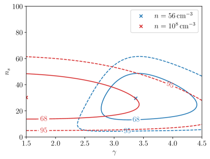
In Fig. 2a, we compare the best-fit results from our analysis and those from SkyLLH Bellenghi et al. (2023) and the most recent analysis of NGC 1068 from IceCube Abbasi et al. (2022). The SkyLLH analysis best-fit parameters are within 2 of our best-fit points. This is expected as both analyses use similar methods and data from the IceCube public release however we only use the events from the full 86 string configuration whereas SkyLLH uses the full 10 year dataset. In Fig. 2b, we also show how the contour for the initial flux parameters is affected by the inclusion of relic neutrino scattering effects. We have specifically chosen a neutrino density value corresponding to a negative value of . The number of signal events is almost identical for this value, , but the spectral index has become small. On the other hand, the 1 range almost contains the best-fit parameter for the original best-fit, which shows that the spectral index may play a sub-dominant role in the final likelihood. When investigating the origin of the slight preference for particular values of the relic density, we found that the lack of statistics at higher muon energies allowed for ambiguities in the analysis. We believe these values will become constrained with improved statistics at higher energies or at least have non-negative values.