James-Stein Estimation in Guassian Metrology : V2
James-Stein Estimation in Quantum Gaussian Sensing
Abstract
The James-Stein estimator is a biased estimator—for a finite number of samples its expected value is not the true mean. The maximum-likelihood estimator (MLE), is unbiased and asymptotically optimal. Yet, when estimating the mean of or more normally-distributed random variables, the James-Stein estimator has a smaller total (expected) error than the MLE. We introduce the James-Stein estimator to the field of quantum metrology, from both the frequentist and Bayesian perspectives. We characterise the effect of quantum phenomena on the James-Stein estimator through the lens of quantum Gaussian sensing, the task of estimating the mean of an unknown multivariate quantum Gaussian state. We find that noiseless entanglement or coherence improves performance of the James-Stein estimator, but diminishes its advantage over the MLE. In the presence of noise, the James-Stein advantage is restored. Quantum effects can also boost the James-Stein advantage. We demonstrate this by investigating multivariate postselective metrology (generalised weak-value amplification), a strategy that uses quantum effects to measure parameters with imperfect detectors. Simply by post-processing measured data differently, our techniques reduce errors in quantum experiments.
I Introduction
The James-Stein estimator underlies one of the most counterintuitive phenomena in classical statistics [1, 2]. Suppose one wishes to estimate 3 or more independent normally distributed quantities, minimising the total mean-squared error. The most common strategy for such a task is the maximum-likelihood estimator (MLE), which treats each quantity separately. However, Stein [1] showed the surprising result that it is always better to combine the data for each quantity, although the underlying quantities are completely independent. Such estimation strategies are now referred to as James-Stein estimators [2]. We refer to the advantage of the James-Stein estimator over the MLE as the James-Stein advantage.
In this Article, we consider the application of James-Stein estimation to parameters encoded in quantum systems. We focus on the particular case of Gaussian shift models [3], which are the quantum generalisations of a Gaussian distribution with an unknown mean. The central-limit theorem [4] ensures that the mean of many identical, independent measurements of any parameterised state is approximately Guassian. Moreover, quantum local asymptotic normality [3] implies that many copies of any parameterised quantum state may be locally approximated as a Gaussian shift model. Therefore, the study of Gaussian shift models is ubiquitous in quantum metrology. We analyse the James-Stein advantage in commonly studied areas of quantum metrology: noiseless metrology, noisy metrology, Bayesian metrology and metrology with postselection (all defined below). We find that boosting metrology by noiseless techniques, employing entanglement or coherence, generally leads to a decrease in the James-Stein advantage. In practice, noise precludes the achievement of theoretically optimal quantum improvements [5]. We show that in the presence of noise, the James-Stein advantage can be considerable. We demonstrate these results in the frequentist and Bayesian regimes. We also consider other experimental limitations, such as imperfect detectors. In such scenarios, it is advantageous to limit the number of measurements of quantum states via postselective filters (see below). These filters harness use quantum effects [6] to compress the information from many copies of a parameterised quantum state, into (arbitrarily) fewer copies. By utilising such compression, one requires few measurements of quantum states to estimate an unknown parameter. We construct an explicit iterative scheme for postselection of Gaussian states. Analysing this scheme, we find that the James-Stein advantage can be increased by postselective filtering. Moreover, postselective filtering can be improved by James-Stein estimation.
II Preliminaries
II.1 Frequentist parameter estimation
Consider an unknown -dimensional parameter , where is a known parameter space. To estimate , one can sample a random variable whose distribution has a probability density function (pdf) . If takes the value , one denotes the corresponding estimate of by . The function is called an estimator. The performance of an estimator is quantified by its risk:
| (1) |
Using the risk, one can quantify the advantage of one estimator over another at a fixed value of the parameter :
| (2) |
If , it is beneficial to use over when .
In the case of separate observations , one considers a family of estimators ; one for each value of . The sequence quantifies how well an estimation strategy performs with increasing resources. The most commonly studied regime in parameter estimation is the asymptotic limit, where is fixed and [7, 8, 9]. In rough terms, the “best” possible estimator has risk scaling as
| (3) |
where is the Fisher information matrix [10], given by
| (4) |
In the quantum setting [11], a parameter is encoded in some quantum state . Often, one has copies of the same state , in which case . One can extract information by measuring . This involves choosing a POVM [12], , where , and . The measurement and state induce a probability distribution parametrised by :
| (5) |
Once a measurement is chosen, the quantum-parameter-estimation problem has been reduced to a classical problem (where takes values in the set of possible measurement outcomes). The quantum analogue of equation (3) is given by
| (6) |
where is called the Holevo-Cramer-Rao bound; see Ref. [13] for details. Note that the optimal estimation strategy includes optimisation over both measurements and estimators.
II.2 The James-Stein Estimator
A particularly important parameter-estimation problem concerns data that is normally distributed around an unknown parameter: 111Here, the notation denotes a random variable for a given value of . Moreover, means “distributed as”.. Here, denotes the (multivaritate) Gaussian (normal) distribution [14], with mean and covariance matrix . For simplicity we assume that is known, though this assumption can be dropped [15].
For normally distributed data, , an intuitive estimator is the MLE, which aligns the estimate with the observed data: . The MLE’s risk is . Below, we compare the MLE with two types of James-Stein estimators [16]. The first is parameterised by a fixed vector and is given by
| (7) |
where . shrinks the Gaussian random variable towards the vector . The risk of is
| (8) |
where the expectation is taken over [16]. The second term is strictly negative. Thus, for any value of . The advantage of the James-Stein estimator is biggest when is close to and is “large”. Below, we fix , and let . If one expects to be close to (and hence that will perform better than ), one can simply translate the origin to .
Instead of shrinking towards a fixed vector, the second type of James-Stein estimator shrinks towards its mean value. For , let be a vector whose entries are all the mean value of . For , the second type of James-Stein estimator is then given by
| (9) |
with risk
| (10) |
Here, the expectation is evaluated over [16]. The advantage of this James-Stein estimator is bigger the more isotropic is (and the “larger” is). Even if there are no correlations between ’s components, i.e., is diagonal, both and combine the components of in a non-trivial manner.
Since the risks of and have similar forms, it is usually sufficient to consider ; will behave similarly. An exception is given by postselective metrology (section VI), where we show that only is relevant. Otherwise, one should choose or depending on the expected properties of : if is small, use ; if is isotropic, use . If no information about is known, one can use either estimator, or a convex combination of them.
If one receives independent identically distributed normally distributed copies , then the sample mean is also normally distributed: . Thus one can define and : one simply applies each estimator to the sample mean. For the James-Stein estimators, this involves modifying by a factor of in equations (7) and (9). One can see that
| (11) |
for both types of James-Stein estimator222We say that if and have the same asymptotic scaling, i.e. there exist constants such that for sufficiently large .. Thus, the James-Stein advantage diminishes with more data. The MLE and James-Stein estimators all saturate equation (3): they are asymptotically optimal.
II.3 Gaussian states
The most natural application of the James-Stein estimator to quantum metrology arises when measurement outcomes are normally distributed. Thus, we consider Gaussian states [17]—states which are characterised by a “mean” and “variance”, like a Gaussian distribution. More precisely, suppose that the Hilbert space is a tensor product of single-mode Fock spaces. Examples include the Hilbert space of 3-dimensional particles, or a system with optical modes [17]. There are pairs of canonical variables satisfying the canonical commutation relations
| (12) |
We group the canonical variables into a single vector . For a state and vector we define ’s characteristic function [17] by
| (13) |
As in classical probability theory, is completely characterised by [18]. A state is called Gaussian [3] if there exists some vector and some positive semi-definite matrix such that
| (14) |
This is exactly the characteristic function of a classical Gaussian probability distribution [14], where is the mean of the distribution, and is its covariance matrix.
III Unknown Gaussian Channel
In this Section, we consider the application of the James-Stein estimator to estimating the mean of a Gaussian state, encoded by some quantum process. We assume that unknown parameters are encoded by a unitary [19]. In analogy with the number of classical samples from a probability distribution, we define as the number of applications of . Thus, quantifies experimental resources.
Let be a Gaussian state with mean zero and covariance matrix , and let , where
| (15) |
Then, we find that is a Guassian state with mean and covariance matrix .
As and are incompatible, we cannot simultaneously measure them. In Ref. [3], it was shown that this problem can be circumvented with the use of an ancilla Gaussian state . The ancilla has the same Hilbert space as , with canonical variables . We prepare with mean 0 and some covariance matrix . Then, we measure the state with respect to the commuting operators .
We define ; note that the Heisenberg uncertainty relation fundamentally lower bounds how small can be (see Ref. [3] for details). In Appendix A, we show, via a calculation using the Wigner function, that if is a random variable corresponding to the outcome of the aforementioned measurement process, then . Since has a Gaussian distribution we may use the James-Stein estimator.
If we are given copies of the unitary , a “classical” estimation strategy is given by preparing copies of and measuring each separately [20]. One finds that the sample mean has distribution and thus that
| (16) |
The James-Stein risk scales as in equation (11).
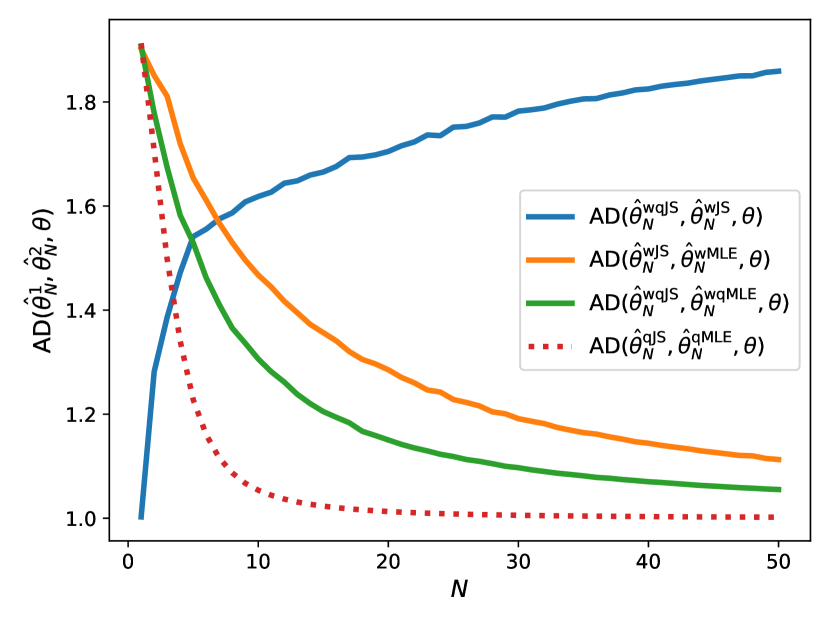
In Ref. [3], it was shown that upon optimisation of , . Thus, the aforementioned measurement combined with the MLE saturates equation (6) and is asymptotically optimal. However, since we note that . Thus, for any finite , the James-Stein estimator has risk smaller than the asymptotic minimum, given in equation (6). The James-Stein advantage must vanish as [as required by equation (6)] but can be substantial for finite ; see Fig. 1 (orange curve).
A common “quantum” strategy [21, 22, 19, 20, 23] is to apply sequentially times to produce the state . Now, is a Gaussian state with covariance matrix and mean . Thus, letting denote the outcome of measuring the mean of , we have .
We denote by and the MLE and James-Stein estimators applied to , respectively. We find that
| (17) |
Using the unitary sequentially gives a factor of improvement over using it on separate copies of . Similarly, , so that the James-Stein estimator is also improved. However, there is a corresponding decrease in the James-Stein advantage compared to equation (11):
| (18) |
In summary, whilst the James-Stein estimator still has an advantage over the MLE, this advantage is suppressed by coherent quantum effects, in the form of sequential unitary applications. See the dotted curve in Fig. 1. The use of an entangled probe state will show similar behaviours.
IV Gaussian Channels with Noise
In Section III, we assumed perfect (noiseless) unitary evolution. In this Section, we lift this assumption and consider a common noise model. We show that the James-Stein and quantum-metrological advantages can be simultaneously large.
Suppose that there is coherent noise, such that we apply instead of , where fluctuates randomly around . This is modelled by the channel
| (19) |
where is the pdf of a normal distribution with mean and covariance matrix . One can check that maps Gaussian states to Gaussian states: if is a Gaussian state with mean and covariance , then is a Gaussian state with mean and covariance . Channels that map Gaussian states to Gaussian states are also called Gaussian [24].
We let denote the sample mean of measuring copies of , and correspond to measuring a single copy of . We find that
| (20) | ||||
| (21) |
We label the estimation strategies , , and applied to the (noisy) variables with a “w” in superscript. We find that the unbounded asymptotic quantum-metrological advantage of equation (17) is reduced to a constant factor:
| (22) |
Nevertheless, we stress that it can still be advantageous to sequentially apply . Depending on the relative size of and , this advantage may be considerable. Moreover, we find that
| (23) |
Comparing equations (18) and (23), we see that the James-Stein advantage is larger in the presence of noise. This is demonstrated in Fig. 1 for a fixed . The blue curve shows that sequentially applying leads to a significant advantage, even in the presence of noise. When , we find that ; a quantum metrological improvement of roughly . From the other curves, we see that the James-Stein advantage falls off less rapidly when is applied sequentially with noise than without noise. When , the James-Stein advantage is about 10% when sequentially applying with noise; it is 1% when sequentially applying without noise. We emphasise that these James-Stein advantages are “free”. No extra experimental resources are required, simply an alternative post-processing of the measured data.
V Bayesian Gaussians
In Bayesian parameter estimation, one assumes that there is some prior distribution on the parameter space that encodes an a priori belief about the parameter to be estimated [4]. With respect to this belief, one can consider the Bayes risk of an estimator :
| (24) |
An estimator is called Bayesian if it minimises the Bayes risk, as defined in equation (24).
We consider the case of a normally distributed prior . To capture the different cases of Sections III and IV, we consider a random variable
| (25) |
where is some full-rank covariance matrix that depends on . We denote the Bayesian, MLE and James-Stein estimators by and , respectively. In Appendix B.1, we show that the Bayes estimator for equation (25) is
| (26) |
We also calculate the Bayes risk of the MLE and James-Stein estimators (see appendix B.2); the results are summarised in Table 1.
By the definition of the Bayes estimator, and since the James-Stein estimator performs better everywhere than the MLE [see equation (11)], we have that
| (27) |
Thus, the Bayes estimator is preferable. However, in practice, one may be unable to use , since it depends explicitly on the covariance matrix , which may be unknown at the point of experiment. Additionally, there is no hope to estimate ; is sampled according to , and subsequently is encoded into copies of . Thus, the copies of yield no information about . Consequently, the James-Stein estimator may be the best available alternative to the Bayes estimator.
If as , then the Bayesian advantage over the MLE is second order in : . Thus, . Moreover, the faster, converges to 0, the faster will converge to 1. Therefore, sequential applications of will move the MLE risk, and hence by equation (27), the James-Stein risk, closer to the optimal Bayes estimator’s risk. That is, the use of quantum-metrological techniques can move the James-Stein risk closer to the unattainable minimal Bayes risk.
VI Postselected Guassian states
In this Section, we consider the application of postselection (defined below) [25, 26, 27, 6] to the estimation of the mean of a Gaussian state. We also investigate how postselection affects the James-Stein advantage. For notational simplicity, we assume that the covariance matrix and that our state is pure. Additionally, by the ancilla trick described in Section III, we may assume that is encoded solely in the positional degree of freedom of our state. That is,
| (28) |
for some known , some unknown , and . For example, this is the state of (continuous-variable) non-entangled, quantum sensors, each estimating some parameter . Given copies of , as detailed in Section III, one could measure the position of each state and take the sample mean to estimate with the corresponding risk scaling as .
Many experiments suffer from limitations such as detector saturation [28, 29, 30, 31] (if the intensity of photons arriving at a photon detector is too high, the detector performance degrades) and dead-times [32, 33, 34] (a detector must reset for a brief time between particle observations). Sometimes, one can only measure of the states produced per unit time. It may be that , so that the rate at which one can measure information is much less than the rate that one can produce it.
If one were to simply discard a random fraction of the copies of , the risk of our estimation strategies would scale as —worse than . However, if one knows that is a small displacement from some known value , i.e. satisfies , then the information carried by probe states can be losslessly compressed down to probe states [25]. This is similar in spirit to weak-value amplification techniques [35, 36, 37, 38, 39, 40, 41, 42, 43, 44, 45, 46, 47].
Instead of discarding states at random, one can utilise a more clever filter described by a 2-outcome POVM, with operators and . The outcome corresponding to (alt. ) has the probe pass (alt. not pass) the filter. Let be a transmission parameter and take
| (29) |
transmits all states perpendicular to , but only allows through with probability . As in [25], we implement with the natural Kraus operator
| (30) |
If a state passes the filter, it will be in the state . In Appendix C.1, we show that if , then the post-filter state of the particle is
| (31) |
Moreover, we show the probability of passing the filter is approximately .
If we measure the probe’s position after postselection, we observe a random variable , approximately normally distributed as
| (32) |
Due to the factor of , is more sensitive in changes to than position measurements of . Thus is distributed as
| (33) |
It takes (on average) copies of until a state passes the filter, but the resulting state has a variance that is smaller than before. Thus, the information in copies of is losslessly compressed into copies of . Such lossless compression has been shown to require genuine quantum effects [6, 25, 46].
We proceed to investigate the advantage of the James-Stein estimator in experiments with post-selective filters. We model the aforementioned situation in which one is limited by a detector. If we can only measure states per unit time, we send copies of through the filter. In this way, we ensure that (on average) states arrive at the detector per unit time. Thus, we can make arbitrarily small (in the approximation ).
We start with with no prior knowledge about and hence no initial guess . This means that is a sub-optimal choice of James-Stein estimator, since we do not expect to be close to any a priori known value. However, if the probes are measuring similar quantities, one could expect that the ’s would be similar and thus that would still perform well. Thus, we only consider in this section, and not . Because we require that , one cannot decrease until one has a good estimate of . We run an iterative strategy (see Appendix C.2 for the algorithm and Appendix C.3 for details on the numerics), where one estimates (using sample variance) and then decreases when one is confident that is sufficiently small. We consider using the MLE or James-Stein estimator to generate our estimates of , and denote these strategies by and , respectively. As a baseline, we compare this to measuring copies of with no postselection (), and using either the MLE or James-Stein estimator .
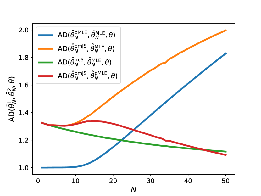
In Fig. 2(a), we fix . The blue curve shows that, when using the MLE, postselection gives an advantage. After some initial few measurements, this advantage increases linearly with the number of measurements. This is due to the increased sensitivity by in the postselected states, which leads to a more accurate estimate of . The orange curve shows that the postselected James-Stein estimator also outperforms the non-postselected MLE. The green (alt. red) curve shows the James-Stein advantage without (alt. with) postselection. We see that using postselection the James-Stein advantage is initially increased, but eventually decays to below the non-postselected James-Stein advantage. This is because using allows one to postselect more quickly, so that the initial advantage increases. However, for larger values of , shrinks, so the sample variance (and hence the James-Stein advantage) decreases. This behaviour is further analysed below. For , postselection boosts the James-Stein advantage.
As discussed above, we expect to perform better when is more “isotropic”. Letting , we quantify ’s isotropy by
| (34) |
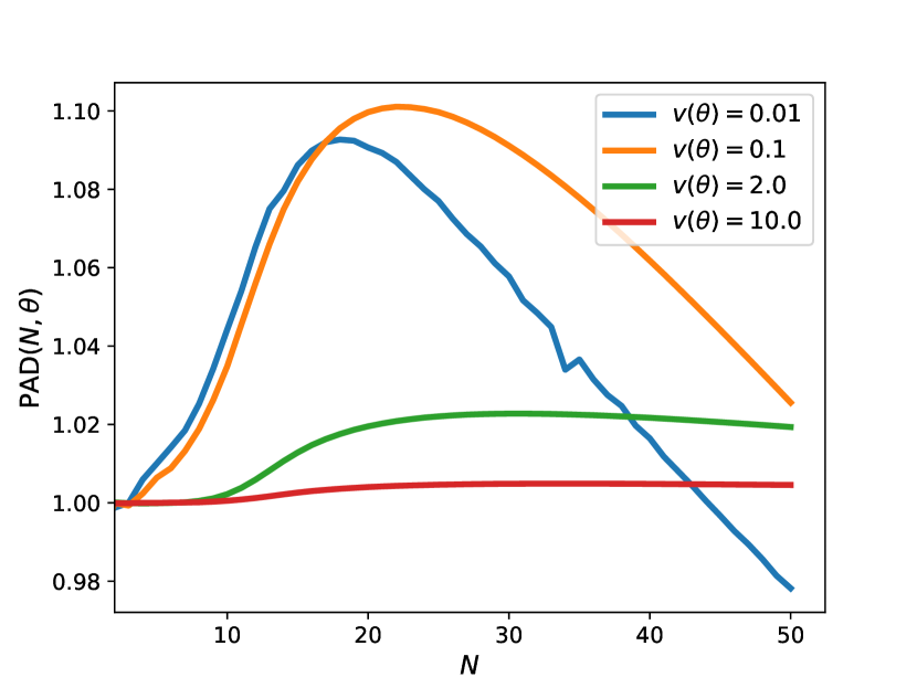
To quantify the effect of postselection on the James-Stein advantage, we consider the ratio
| (35) |
If , then postselection has increased the James-Stein advantage (compared to the non-postselected case). In Fig. 2(b), we plot against for 4 different values of , each with a different . As described above, the James-Stein estimator allows stronger postselection for smaller , so that . However, as increases, the factor in sensitivity increases by a factor of , which degrades the James-Stein advantage. Thus, PAD eventually decreases. These effects are magnified when is smaller.
VII Conclusion
We have introduced the James-Stein estimator to quantum metrology. We have focused on Gaussian shift estimation, but our techniques generalise to most common parameterised quantum states. We have shown that across a wide array of quantum-metrology protocols, the James-Stein estimator outperforms the MLE. This means that by simply changing post-processing techniques, one can increase experimental performance, without requiring any additional experimental resources. Our results highlight the non-trivial relationship between the asymptotic and non-asymptotic regimes of (quantum) metrology [48, 49]; strategies that are asymptotically optimal may be sub-optimal with finite resources. We conclude that the James-Stein estimator can be a useful tool in quantum metrology. Moreover, quantum phenomena have a non-trivial relationship with the James-Stein advantage; they may increase it (sec. VI), diminish it (sec. III), or neither (sec. IV).
Acknowledgements
The authors wish to thank P. Karlsson for prompting them to investigate the James-Stein estimator in a quantum setting. Further, the authors thank N. Mertig, F. Venn, C. Long and J. Smith for their useful discussions and comments. W.S. was supported by the EPSRC and Hitachi. S.S. acknowledges support from the Royal Society University Research Fellowship. D.R.M.A.-S. was supported by Girton College.
References
- Stein [1956] C. Stein, Proceedings of the Third Berkeley Symposium on Mathematical Statistics and Probability 1, 197 (1956).
- Stein and James [1961] C. Stein and W. James, Proceedings of the Fourth Berkeley Symposium on Mathematical Statistics and Probability 1, 361 (1961).
- Demkowicz-Dobrzański et al. [2020] R. Demkowicz-Dobrzański, W. Górecki, and M. Guţă, Journal of Physics A: Mathematical and Theoretical 53, 363001 (2020).
- Wasserman [2004] L. Wasserman, All of Statistics (Springer, New York, NY, 2004) p. 202.
- Demkowicz-Dobrzański et al. [2012] R. Demkowicz-Dobrzański, J. Kołodyński, and M. Guţă, Nature communications 3, 1063 (2012).
- Arvidsson-Shukur et al. [2020] D. R. M. Arvidsson-Shukur, N. Yunger Halpern, H. V. Lepage, A. A. Lasek, C. H. W. Barnes, and S. Lloyd, Nat. Commun. 11, 3775 (2020).
- Lehmann and Casella [1998] E. L. Lehmann and G. Casella, Theory of Point Estimation (Springer, New York, NY, 1998).
- Braunstein and Caves [1994] S. L. Braunstein and C. M. Caves, Phys. Rev. Lett. 72, 3439 (1994).
- Albarelli et al. [2020] F. Albarelli, M. Barbieri, M. Genoni, and I. Gianani, Physics Letters A 384, 126311 (2020).
- Vaart [1998] A. W. v. d. Vaart, Efficiency of estimators, in Asymptotic Statistics, Cambridge Series in Statistical and Probabilistic Mathematics (Cambridge University Press, 1998) p. 108–124.
- Helstrom [1969] C. W. Helstrom, Journal of Statistical Physics 1, 231 (1969).
- Nielsen and Chuang [2010] M. A. Nielsen and I. L. Chuang, Quantum Computation and Quantum Information: 10th Anniversary Edition (Cambridge University Press, 2010).
- Yang et al. [2019] Y. Yang, G. Chiribella, and M. Hayashi, Communications in Mathematical Physics 368, 223 (2019).
- van der Vaart [2000] A. W. van der Vaart, Asymptotic Statistics (Cambridge University Press, 2000).
- Chételat and Wells [2012] D. Chételat and M. T. Wells, The Annals of Statistics 40, 3137 (2012).
- Li and Bhoj [1988] T. F. Li and D. S. Bhoj, Scandinavian Journal of Statistics 15, 33 (1988).
- Weedbrook et al. [2012] C. Weedbrook, S. Pirandola, R. García-Patrón, N. J. Cerf, T. C. Ralph, J. H. Shapiro, and S. Lloyd, Rev. Mod. Phys. 84, 621 (2012).
- Englert and Wódkiewicz [2003] B.-G. Englert and K. Wódkiewicz, International Journal of Quantum Information 1, 153 (2003).
- Giovannetti et al. [2006] V. Giovannetti, S. Lloyd, and L. Maccone, Phys. Rev. Lett. 96, 010401 (2006).
- Giovannetti et al. [2011] V. Giovannetti, S. Lloyd, and L. Maccone, Nature Photonics 5, 222 (2011).
- Smith et al. [2022a] J. G. Smith, C. H. W. Barnes, and D. R. M. Arvidsson-Shukur, Phys. Rev. A 106, 062615 (2022a).
- Smith et al. [2022b] J. G. Smith, C. H. W. Barnes, and D. R. M. Arvidsson-Shukur, Phys. Rev. A 106, 062615 (2022b).
- Ji et al. [2008] Z. Ji, G. Wang, R. Duan, Y. Feng, and M. Ying, IEEE Transactions on Information Theory 54, 5172 (2008).
- Eisert and Wolf [2007] J. Eisert and M. M. Wolf, Quantum Information with Continous Variables of Atoms and Light 10.48550/ARXIV.QUANT-PH/0505151 (2007).
- Jenne and Arvidsson-Shukur [2022] J. H. Jenne and D. R. M. Arvidsson-Shukur, Unbounded and lossless compression of multiparameter quantum information (2022).
- Salvati et al. [2023] F. Salvati, W. Salmon, C. H. Barnes, and D. R. Arvidsson-Shukur, arXiv preprint arXiv:2307.08648 (2023).
- Lupu-Gladstein et al. [2022a] N. Lupu-Gladstein, Y. B. Yilmaz, D. R. Arvidsson-Shukur, A. Brodutch, A. O. Pang, A. M. Steinberg, and N. Y. Halpern, Physical Review Letters 128, 220504 (2022a).
- Luu and Jiang [2006] J. X. Luu and L. A. Jiang, Applied optics 45, 3798 (2006).
- Wang et al. [2010] J. Wang, T. Liu, S. Jiao, R. Chen, Q. Zhou, K. K. Shung, L. V. Wang, and H. F. Zhang, Journal of biomedical optics 15, 021317 (2010).
- Frehlich and Ochs [1990] R. G. Frehlich and G. R. Ochs, Applied optics 29, 548 (1990).
- Lupu-Gladstein et al. [2022b] N. Lupu-Gladstein, Y. B. Yilmaz, D. R. M. Arvidsson-Shukur, A. Brodutch, A. O. T. Pang, A. M. Steinberg, and N. Y. Halpern, Phys. Rev. Lett. 128, 220504 (2022b).
- Hachisu and Ido [2015] H. Hachisu and T. Ido, Japanese Journal of Applied Physics 54, 112401 (2015).
- Wahl et al. [2020] M. Wahl, T. Röhlicke, S. Kulisch, S. Rohilla, B. Krämer, and A. C. Hocke, Review of Scientific Instruments 91 (2020).
- Rohde and Ralph [2006] P. P. Rohde and T. C. Ralph, Journal of Modern Optics 53, 1589 (2006).
- Hosten and Kwiat [2008] O. Hosten and P. Kwiat, Science 319, 787 (2008).
- Dixon et al. [2009] P. B. Dixon, D. J. Starling, A. N. Jordan, and J. C. Howell, Phys. Rev. Lett. 102, 173601 (2009).
- Turner et al. [2011] M. D. Turner, C. A. Hagedorn, S. Schlamminger, and J. H. Gundlach, Opt. Lett. 36, 1479 (2011).
- Pfeifer and Fischer [2011] M. Pfeifer and P. Fischer, Opt. Express 19, 16508 (2011).
- Starling et al. [2010a] D. J. Starling, P. B. Dixon, A. N. Jordan, and J. C. Howell, Phys. Rev. A 82, 063822 (2010a).
- Starling et al. [2010b] D. J. Starling, P. B. Dixon, N. S. Williams, A. N. Jordan, and J. C. Howell, Phys. Rev. A 82, 011802 (2010b).
- Xu et al. [2013] X.-Y. Xu, Y. Kedem, K. Sun, L. Vaidman, C.-F. Li, and G.-C. Guo, Phys. Rev. Lett. 111, 033604 (2013).
- Magaña-Loaiza et al. [2014] O. S. Magaña-Loaiza, M. Mirhosseini, B. Rodenburg, and R. W. Boyd, Phys. Rev. Lett. 112, 200401 (2014).
- Strübi and Bruder [2013] G. Strübi and C. Bruder, Phys. Rev. Lett. 110, 083605 (2013).
- Viza et al. [2013] G. I. Viza, J. Martínez-Rincón, G. A. Howland, H. Frostig, I. Shomroni, B. Dayan, and J. C. Howell, Opt. Lett. 38, 2949 (2013).
- Egan and Stone [2012] P. Egan and J. A. Stone, Opt. Lett. 37, 4991 (2012).
- Pusey [2014] M. F. Pusey, Phys. Rev. Lett. 113, 200401 (2014).
- Kunjwal et al. [2019] R. Kunjwal, M. Lostaglio, and M. F. Pusey, Physical Review A 100, 042116 (2019).
- Salmon et al. [2023] W. Salmon, S. Strelchuk, and D. Arvidsson-Shukur, Quantum 7, 998 (2023).
- Meyer et al. [2023] J. J. Meyer, S. Khatri, D. S. França, J. Eisert, and P. Faist, arXiv preprint arXiv:2307.06370 (2023).
- Tatarskiĭ [1983] V. I. Tatarskiĭ, Soviet Physics Uspekhi 26, 311 (1983).
- Banerjee et al. [2005] A. Banerjee, X. Guo, and H. Wang, IEEE Transactions on Information Theory 51, 2664 (2005).
- Casella et al. [2004] G. Casella, C. P. Robert, and M. T. Wells, Lecture Notes-Monograph Series , 342 (2004).
Appendix A Distribution of Gaussian measurement outcome
In this appendix, we find the distribution of the measurement described in Section III (and Ref. [3]). We begin by recapping the definition of a Gaussian state. Let be the tensor product of single mode Fock spaces. Let be a vector of operators, where are the position and momentum canonical variables of the th system, so that
| (36) |
The characteristic function of a state is the function
| (37) |
A state is called Gaussian if for some and some positive semi-definite matrix, we have that
| (38) |
The Wigner function [50] of the state is defined as the Fourier transformation of the characteristic function, that is
| (39) |
If is a Gaussian state, then we find that
| (40) |
i.e. a Gaussian in phase space.
As in Section III, suppose we have a Gaussian state with a known covariance matrix , but unknown mean that we wish to estimate. That is
| (41) |
We cannot simultaneously measure the position and the momentum of the state, but detailed in Ref. [3], we can circumvent this problem with the use of an ancilla. The ancilla is in a Gaussian state which has the roles of position and momentum inverted. That is to say we define a vector of operators
| (42) |
and ask that satisfies
| (43) |
for some vector and covariance matrix .
Defining the swap matrix
| (44) |
we find that is a Gaussian state with mean vector and covariance matrix .
The joint state has Wigner function
| (45) |
where
| (46) |
Ref. [3] notes that the operators
| (47) |
mutually commute, and thus can be simultaneously measured. In fact, they show that this measurement scheme is optimal—the Fisher information of the resulting distribution is maximal.
Consider the probability density at the measurement outcome , , denoted . Using standard properties of the Wigner function (see Ref. [50] for details), we find
| (48) | ||||
| (49) |
where
| (50) |
We wish to extract the and dependence from this integral. Let , and . Using the definition of and , we find that
| (51) |
We complete the square in the exponent, i.e. write it in the form
| (52) |
for some . From inspection, we can see that
| (53) |
This gives
| (54) | ||||
| (55) |
where the matrices are given by
| (56) |
In fact, all of the are equal, as we show in the following lemma.
Lemma A.1.
.
Proof: By symmetry of the it suffices to prove the claim for and . Note
| (57) |
Additionally,
| (58) | ||||
| (59) |
The result follows. ∎
Appendix B Bayesian Gaussian calculations
In this appendix, we find the Bayes estimator for the measurement process described in Section V, as well as the Bayes risk of the maximum-likelihood, James-Stein and Bayes estimators
B.1 Finding the Bayes estimator
Recall that we are considering the (classical) Bayesian estimation problem of and . Since we are using least squares loss [51], the Bayes estimator has the simple form
| (62) |
Thus, consider the distribution of .
| (63) |
Note
| (64) |
We complete the square in the exponent, i.e. write it in the form
| (65) |
From inspection, it is clear that we need
| (66) |
We deduce
| (67) |
so that . We also find that
| (68) |
In analogy with equation (54) we find that
| (69) |
And thus deduce
| (70) |
B.2 Calculating Bayes risks
We recall the three estimators we are comparing:
| (71) |
Since , it is easy to see .
From equation (II.2) we know
| (72) |
By definition,
| (73) |
so using the tower law of expectation we find
| (74) |
where the expectation is now taken over the full distribution of that we found in equation (70).
It remains to find the Bayes-risk of the Bayes estimator . Using by the tower-law of expectation,
| (75) |
Since and is distributed according to equation (67), the inner expectation is the expected squared distance of a multivariate Gaussian distribution from its mean, which is the trace of the covariance matrix: . The outer expectation is then the expectation of a constant so that
.
In order to compare the Bayes risk of the Bayes estimator with the MLE and JS risks, it is useful to rewrite this risk using lemma A.1. Taking and . We find
| (76) |
Noting that is symmetric, and is positive definite, we deduce that that .
Appendix C Postselection
C.1 Approximate postselected state
In this appendix, we justify equation (31) in Section VI. First we calculate the overlap
| (77) | ||||
| (78) | ||||
| (79) |
Then
| (80) | ||||
| (81) | ||||
| (82) | ||||
| (83) |
We can see from equation (82) that the integrand only has effective support for . Thus we can Taylor expand in , treating as .
| (84) | ||||
| (85) | ||||
| (86) | ||||
| (87) |
So for , we find, as claimed in the main text, that
| (88) |
C.2 Iterative Strategy
In this appendix, we describe our iterative strategy for estimating using postselection. We wish to compare the James-Stein estimator and MLE. In order to capture both cases, we describe the algorithm in more general terms, referring only to an estimator for estimating the mean of a Gaussian distribution. If one wishes to implement a specific strategy, one can replace by, for example, or .
Initially, we set and .
Suppose we are on the th measurement; and have been set to some known values. Recall (from appendix C.1), that the postselected state is roughly
| (89) |
We measure the position of the postselected state, let the outcome be . Rescaling, we take so that . We make an estimate of . Our collated estimate (using all the data so far) is given by , the sample mean of . Denote the sample standard deviation of by . We estimate by .
If is ever less than , we set to and to : our current best estimate of .
If the strategy terminates after measurement , we output . Thus, after measurement , the current error of the estimation strategy is given by . To estimate the risk of a particular strategy or at measurement , we average over many individual repetitions.
C.3 Exact sampling from the postselected pdf
In order to numerically simulate the postselection, we must sample exactly from the distribution
| (90) |
given by measuring the position of the postselected state.
In order to do this, we use rejection sampling. We give a brief summary of rejection sampling here, for details see Ref. [52]. Assume there is a target pdf that we wish to sample from. Rejection sampling requires a pdf that one can sample from, and constant satisfying . The rejection sampling algorithm is:
-
1.
Generate a candidate from the pdf .
-
2.
Output this candidate with probability . If the candidate is rejected, return to step 1.
Note that the chance of acceptance is given by . Thus, on average, samples from are required to generate one sample from .
To use rejection sampling, we must find a constant and a pdf that is easy to sample from, such that . First, we calculate
| (91) |
where . Then, recalling , we find
| (92) |
By expanding the square and integrating each of the resulting Gaussians, we find that
| (93) | ||||
| (94) |
If , note that . Thus, we may bound equation (92) by
| (95) |
Thus,
| (96) | ||||
| (97) | ||||
| (98) |
where
| (99) |
and
| (100) |
Note that is a pdf given by the convex sum of the pdf of two different normal distributions. Specifically, let
| (101) |
denote the pdf of a normal distribution with mean and covariance matrix . Then,
| (102) |
where
| (103) |
Thus it is easy to sample from : sample from with probability , otherwise sample from . Therefore, we can use rejection sampling to sample from . Note that as , so as postselection becomes stronger, rejection sampling takes longer (on average) to run.