Measuring White Dwarf Variability from Sparsely Sampled Gaia DR3 Multi-Epoch Photometry

Abstract

White dwarf stars are ubiquitous in the Galaxy, and are essential to understanding stellar evolution. While most white dwarfs are photometrically stable and reliable flux standards, some can be highly variable, which can reveal unique details about the endpoints of low-mass stellar evolution. In this study we characterize a sample of high-confidence white dwarfs with multi-epoch photometry from Gaia Data Release 3. We compare these Gaia light curves with light curves from the Zwicky Transiting Facility and the Transiting Exoplanet Survey Satellite to see when Gaia data independently can accurately measure periods of variability. From this sample, 105 objects have variability periods measured from the Gaia light curves independently, with periods as long as roughly 9.5 d and as short as 256.2 s (roughly 4 min), including seven systems with periods shorter than 1000 s. We discover 86 new objects from the 105 target sample, including pulsating, spotted, and binary white dwarfs, and even a new 68.4 min eclipsing cataclysmic variable. The median amplitude of the absolute photometric variability we confirm from Gaia independently is 1.4%, demonstrating that Gaia epoch photometry is capable of measuring short-term periods even when observations are sparse.

1 Introduction

As the endpoints of all stars below roughly 8 $M_{\odot}$, white dwarfs are extremely common. Their ubiquity and relative simplicity mean that white dwarf stars play an important role as flux standards, which are needed for precise absolute photometry and spectroscopy (e.g., Calamida et al., 2022).

Roughly 97% of all apparently isolated white dwarfs are empirically stable to less than 1% variability on weeks-long timescales (Hermes et al., 2017a). When white dwarfs are photometrically variable they can reveal unique physical properties such as the presence of magnetism or surface rotation periods (e.g., Maoz et al., 2015), binary properties (e.g., Holberg & Howell, 2011), remnant planetary systems (e.g, Hallakoun et al., 2018; Guidry et al., 2021), or even their interiors through asteroseismology (e.g., Romero et al., 2012).

Binary systems with at least one white dwarf star can tell us about stellar ages and close binary evolution (e.g., Rebassa-Mansergas et al. 2007; Heintz et al. 2022). These objects can also be progenitors of Type Ia supernovae, which are important distance indicators (Maoz et al., 2015). Binaries with short periods (less than roughly 1 hour) are also potential candidates for gravitational waves detectable with the Laser Interferometer Space Antenna (LISA, Burdge et al. 2020).

There are a number of ways binaries with a white dwarf can be photometrically variable. Eclipsing systems are the most dramatic, where one star passes in front of the other (e.g., Hallakoun et al. 2016). Eclipsing white dwarfs, which can be used to measure the masses and radii of the system components (Parsons et al., 2017, 2018), are still relatively rare so any increase in the sample is valuable. Eclipses are not necessary to detect close binaries, as hot stars in the system can create a reflection effect from reprocessed heating off a cool companion (e.g., Schaffenroth et al. 2022). In addition, cataclysmic variables (CVs) are highly variable white dwarfs with stochastic mass-transfer from a Roche-lobe-filling main-sequence companion (Warner, 1995).

Magnetic white dwarfs can also exhibit strong photometric changes, such as cold (e.g., Brinkworth et al. 2013; Kilic et al. 2015) or hot (e.g., Hoard et al. 2018) spots corresponding to the surface rotation period. Measuring these rotation periods can help to investigate the angular momentum loss during white dwarf formation (Fuller et al., 2019).

Pulsating white dwarfs are variable due to non-radial pulsations as they cool through different instability strips that depend on their surface composition (Winget & Kepler, 2008a; Fontaine & Brassard, 2008; Hermes et al., 2017c). With enough identified pulsation modes, asteroseismology affords the opportunity to significantly constrain the interiors of white dwarfs, including global rotation rates (e.g., Hermes et al. 2015, 2017b) and core composition (e.g., Giammichele et al. 2018; Chidester et al. 2022).

Motivated by the need to find and constrain new variable white dwarfs, we analyze here a new data product from Gaia Data Release 3 (DR3), which features multi-epoch light curves for sources classified as variable via a machine learning algorithm trained on constant objects (Eyer et al., 2023). This new Gaia DR3 dataset includes photometric time series in the Gaia $G$, $G_{\mathrm{BP}}$, and $G_{\mathrm{RP}}$ bands. Previous efforts have focused on literature cross-matches of DR3 variables (Gavras et al., 2023; Rimoldini et al., 2023), as well as specific object types (Gaia Collaboration et al., 2023a; Marton et al., 2023).

In Section 2 we discuss our target selection for variable white dwarfs in Gaia DR3, and in Section 3 describe our period-finding analysis. In Section 4 we explain our classification of new white dwarf variables, including new (eclipsing) binaries, spotted (magnetic) white dwarfs, and pulsating white dwarfs, all with coherent periodicities detected from Gaia DR3 photometry independently and confirmed in multiple datasets. We discuss the strengths and limitations of Gaia for period analysis in Section 5 and conclude in Section 6.

2 Target Selection and Observations

We set out to select and analyze all apparently isolated white dwarf stars flagged as photometrically variable in Gaia DR3 (Gaia Collaboration et al., 2023b). A new, expanded data product in DR3 is the release of multi-epoch, multi-color ($G$, $G_{\mathrm{BP}}$, $G_{\mathrm{RP}}$) light curves for roughly 10.5 million objects with anomalously large scatter in their many Gaia visits (a.k.a. transits) that make them high-probability candidate variables (Eyer et al., 2023). These objects are cataloged in Gaia DR3 with the entry phot_variable_flag set to VARIABLE; full light curves are available through the Gaia Datalink Service (Cánovas & de Bruijne, 2022), which we accessed using astroquery.gaia (Ginsburg et al., 2019).

In order to focus on isolated white dwarfs, we first restrict the 10.5 million variables in DR3 to be near the white dwarf region of the Gaia color-magnitude diagram by requiring $M_{G}>(4.5\times G_{\mathrm{BP}}-G_{\mathrm{RP}})+9.0$, similar to the absolute magnitude selection of Hollands et al. (2018). This excludes many white dwarfs in close binaries, such as CVs (Pala et al., 2020) and post-common-envelope (WD+dM) binaries.

We then cross-match this down-selected sample with the Gaia DR3 catalog of candidate white dwarfs of Gentile Fusillo et al. (2021). This cross-match results in a final sample of 1333 objects, 1217 of which are high-confidence single white dwarfs (with $P_{{\mathrm{W}D}}>0.75$, see Table 1); only 42 objects have $P_{{\mathrm{W}D}}<0.3$. We expect minor contamination from our color cuts from non-isolated white dwarfs, especially CVs with low-luminosity donors.

We further cross-match this sample with the Montreal White Dwarf Database (Dufour et al., 2017) and SIMBAD (Wenger et al., 2000) by matching coordinates for each source (precessing the Gaia DR3 epoch to J2000). This cross-match was done in order to collect as much supporting information as possible including literature references and spectroscopic classifications. Relevant information found in this cross match is listed in Table Measuring White Dwarf Variability from Sparsely Sampled Gaia DR3 Multi-Epoch Photometry.

We compare the Gaia multi-color light curves of our 1333 objects with two other long-baseline photometric surveys. First, we use the Python package Lightkurve (Lightkurve Collaboration et al., 2018; Saunders, 2020) to download any 20-second- and 2-min-cadence PDCSAP light curves of our objects as seen by the Transiting Exoplanet Survey Satellite (TESS, Ricker et al. 2015). This provides at least one month of nearly continuous TESS data for 698 objects in our sample, most brighter than roughly $G=17.0$ mag.

Where available, we also download light curves within a 1.4-arcsecond search radius of our targets from Data Release 12 of the Zwicky Transient Facility (ZTF, Bellm et al. 2019). This provides long-baseline ZTF observations for 992 objects across all magnitudes in our sample, all with declinations north of $-20$ degrees. We also search for light curves in the south from the All-Sky Automated Survey for SuperNovae (ASAS-SN, Shappee et al. 2014; Kochanek et al. 2017) and the Asteroid Terrestrial-impact Last Alert System (ATLAS, Tonry et al. 2018) projects. However, any objects without TESS photometry in the south mostly had upper limits on photometry due to their faintness, so we did not use their light curves in our analysis here.

3 Period-Finding Analysis

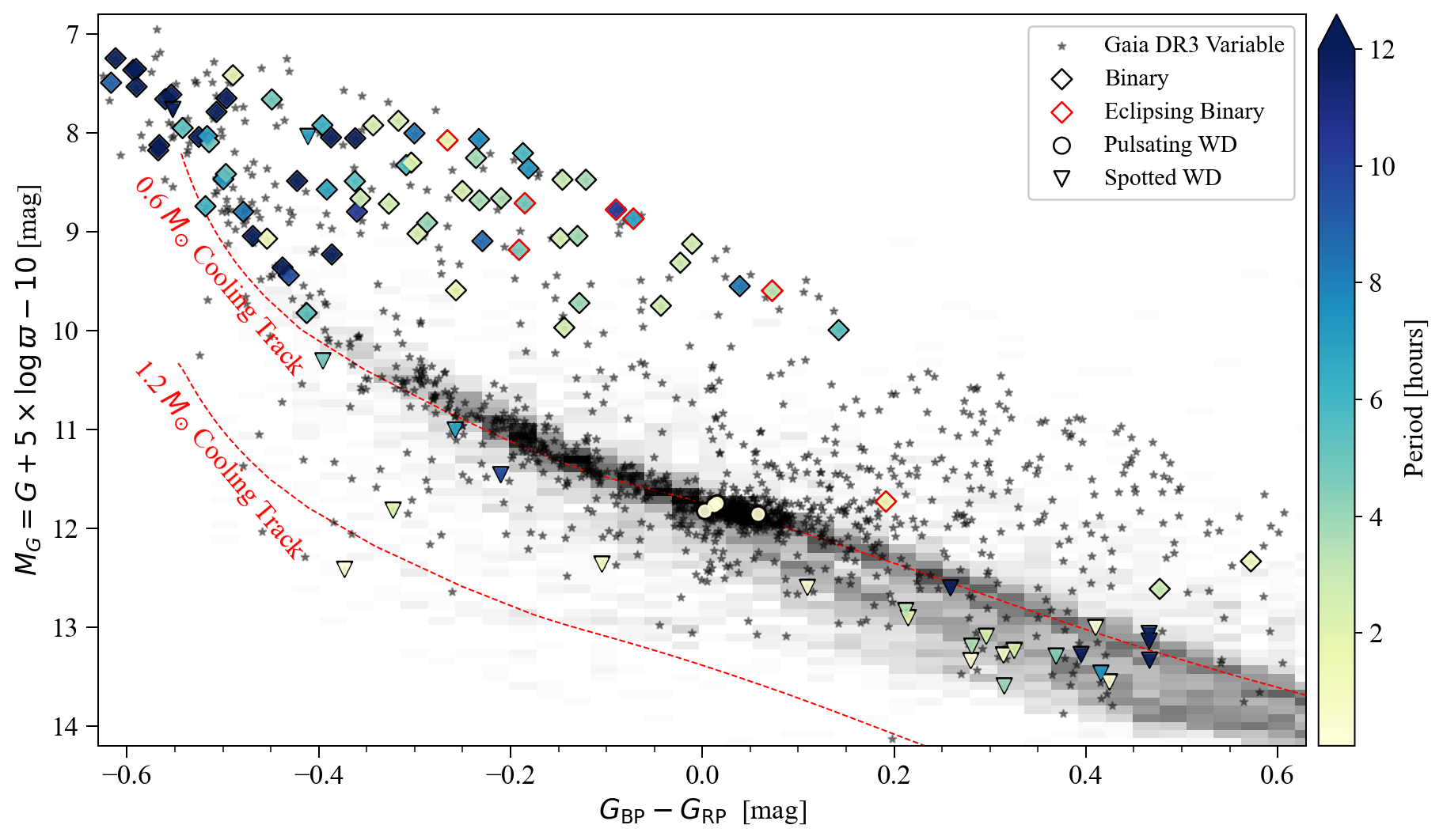
Figure 1: Color-magnitude diagram showing our sample of 1333 high-confidence white dwarf candidates flagged as photometrically variable in Gaia DR3 as black stars. The larger colored symbols show the 105 objects discussed in this manuscript which have variability periods measured from their Gaia light curves independently; the color for each point corresponds to the corresponding variability period. The background of this plot is a two-dimensional histogram of white dwarfs within 200 pc matching the magnitude distribution of the 1333 photometrically variable white dwarfs. Dashed red lines show the expected cooling tracks of a 0.6 $M_{\odot}$ white dwarf at top and 1.2 $M_{\odot}$ white dwarf at bottom; white dwarfs cool from the upper left to the lower right in this diagram.

We analyze the Gaia light curves and ZTF and TESS light curves, when available, simultaneously. All available light curves are visually inspected for signatures of variability in both the time and frequency domain, informed by the spectroscopic classification of the white dwarf if known.

We analyze every light curve in the frequency domain by computing Lomb-Scargle periodograms (Astropy Collaboration et al., 2013) using astropy (Astropy Collaboration et al., 2013, 2018, 2022). We also separate the light curves by band-pass filters ($G$, $G_{\mathrm{BP}}$, $G_{\mathrm{RP}}$, $g$, $r$, $T$ from Gaia, ZTF, and TESS, respectively) to search for color-dependant variability. We initially classify frequencies as significant if their amplitude exceeds five times the mean amplitude of all frequencies in the periodogram, a relatively conservative limit given prior sporadically sampled datasets (Breger et al., 1993; Guidry et al., 2021). For simplicity, we use a constant frequency step size for Gaia and ZTF data: $10^{-8}$ Hz, which corresponds to a critical sampling of 1157 days, consistent with the length of the typical Gaia and ZTF datasets. The step size for the TESS periodogram frequencies is set by the inverse of the TESS light curve baseline, oversampled by a factor of 10. All periodograms are computed to the TESS 2-min Nyquist frequency of 4160 $\mu$Hz.

We use all available survey information in addition to our coherent period analysis to attempt to classify as many variable candidate white dwarfs in our sample as possible (see Figure 1 and top-line summary in Table 1). The amount of information differs significantly from source to source. For example, only 586 of 1333 objects have a spectral type in the literature listed from either MWDD (Dufour et al., 2017) or SIMBAD (Wenger et al., 2000). Therefore, our classification for 86 of 105 objects in Table Measuring White Dwarf Variability from Sparsely Sampled Gaia DR3 Multi-Epoch Photometry listed as “likely” is based on the limited information available and requires spectroscopic follow-up to truly confirm the variability classification.

Most variables are categorized by their periods of variability (from $100-1500$ s for pulsating white dwarfs, to minutes to days for spotted white dwarfs), as well as their position in the color-magnitude diagram (e.g., CVs are composed of a composite spectra mixing some fraction of a white dwarf, main-sequence star, and accretion disk, and are considerably over-luminous to an isolated white dwarf). Using the color-magnitude position along with any periods constrained from the survey light curves allows us to suggest likely classifications for the subset of objects in this manuscript; we will present full classification of all 1333 objects in a future publication.

We devote our attention here to objects where at least one Gaia light curve successfully identifies the period of variability of a candidate white dwarf. We consider Gaia to successfully recover a period if the Gaia-$G$ periodogram has its highest peak matching (to within 0.05 $\mu$Hz) the highest peak of an independent ZTF and/or TESS periodogram, or an independent Gaia bandpass light curve.

Regardless of its significance (we discuss further in Section 5), we use the highest-amplitude of the periodogram of the available Gaia, ZTF, and TESS datasets as an initial guess for a linear-least-squares (LLS) fit of a sinusoid to the data using the Python package lmfit (Newville et al., 2016). This process returns the best-fit period, amplitude, and phase of a single sinusoid to the light curve, as well as associated uncertainties. All reported periods in the main text of this manuscript are the LLS fits of the Gaia DR3 $G$-band photometry.

Table 1: Summary table of the full sample and a subset of Gaia-detected variable candidate white dwarfs.

	Full Sample	Gaia Period Match
Variable objects near white dwarfs in CMD (”Variable candWDs”)	1333	105
Candidate WDs with $P_{\rm WD}>0.75$	1217	104
Variable candWDs with spectroscopic confirmation	568	36
Variable candWDs that are known binaries	91	8
Variable candWDs that are known pulsating WDs	49	2
Variable candWDs known to have magnetic spots	12	8
Variable candWDs with TESS data	698	65
Variable candWDs with ZTF data	992	72

In total we find 105 candidate white dwarfs which have photometric variability periods that can be correctly measured from their Gaia DR3 light curve independently. Of these 105 objects, 72 have data from ZTF and 65 have data from TESS (including 32 with both ZTF and TESS data). Based on our classification (see Section 4), we show where these 105 objects sit in the Gaia color-magnitude diagram in Figure 1. Because binary systems and objects with cool spots both show sinusiodal variability, we use mass and temperature estimate fits to Gaia photometry by Gentile Fusillo et al. (2021) (listed in Table Measuring White Dwarf Variability from Sparsely Sampled Gaia DR3 Multi-Epoch Photometry) to distinguish between these objects. We classify candidate white dwarfs with an effective temperature of $>$ $31{,}000$ K or a photometrically determined mass $<$ $0.525$ $M_{\odot}$ (which cannot have formed as single-stars within a Hubble time) as binaries; all other sinusoidally variable white dwarfs are classified as rotationally modulated spots. Since not all spotted white dwarfs are strongly magnetic (e.g., Hermes et al. 2017b), the only way to absolutely distinguish between a spot or binary is to use follow-up spectroscopy to search for radial-velocity variability.

Previous spectroscopy exists for just 36 of our 105 targets. Our photometric classifications lacking spectroscopic constraints will suffer some ambiguity. For example, WD J202932.51$+$070107.70 is hotter than $31{,}000$ K and exhibits absorption from ultra-highly excited metals, but is likely variable due to a magnetic spot (Reindl et al., 2021). Similarly, the $>$ $100{,}000$ K white dwarf WD J095125.94$+$530930.72 is likely spotted, based on a lack of radial-velocity variation (Werner et al., 2019). Still, classifying as binaries the sinusoidal variables with ${T}_{\mathrm{eff}}$ $>$ $31{,}000$ K or ${M}_{\mathrm{WD}}<$ $0.525$ $M_{\odot}$ will be appropriate for the vast majority of our objects.

4 Classified white dwarf variables

We attempt to classify the origin of the variability for the 105 candidate variable white dwarfs where we can measure a coherent, sinusoidal variability period from the Gaia light curves that matches a period detected in an independent dataset. Initially we inspect the Gaia DR3 machine learning output classifier (GaiaDR3Class), which is available for 62/105 objects. In most cases, however, this classifier simply says WD, revealing little about the specific nature of these objects.

We instead classify all objects based on variability period and position in the Gaia color-magnitude diagram, informed by past white dwarf variability studies (Hermes et al., 2017a; Reding et al., 2018). All discovery literature on our sources is collected in Table Measuring White Dwarf Variability from Sparsely Sampled Gaia DR3 Multi-Epoch Photometry, and our full classification and variability information is collected in Table Measuring White Dwarf Variability from Sparsely Sampled Gaia DR3 Multi-Epoch Photometry. Table 1 provides a summary of the overall sample and our analyzed sub-sample referenced in this manuscript.

4.1 Non-Eclipsing White Dwarf Binaries

Binary systems are often distinguishable from isolated white dwarfs because they are an unresolved pair of stars, making them over-luminous to single star cooling tracks, such as those shown in Figure 1. For this reason, over-luminous objects with sinusiodal variability that have an effective temperature exceeding $31{,}000$ K as determined by the hydrogen-rich-atmosphere fits from Gentile Fusillo et al. (2021) or a photometrically determined mass $<0.525$ $M_{\odot}$ are categorized as binary systems. Objects without mass determinations from Gentile Fusillo et al. (2021) are likely over-luminous and also classified as binaries. Typical values for orbital periods of binary systems with a white dwarf paired with an M dwarf have been studied by Nebot Gómez-Morán et al. (2011), where SDSS data showed that post common envelope binaries containing a white dwarf and main sequence star have orbital periods ranging from 1.9 hr to 103.2 hr, with an average of approximately 10.3 hr.

We find 72 likely variable binaries in our sample, including seven eclipsing binaries (Section 4.3), with orbital periods ranging from 0.957 hr to 29.366 hr, with a mean of approximately 8.411 hr and a standard deviation of approximately 7.417 hr, consistent with the Nebot Gómez-Morán et al. (2011) distribution.

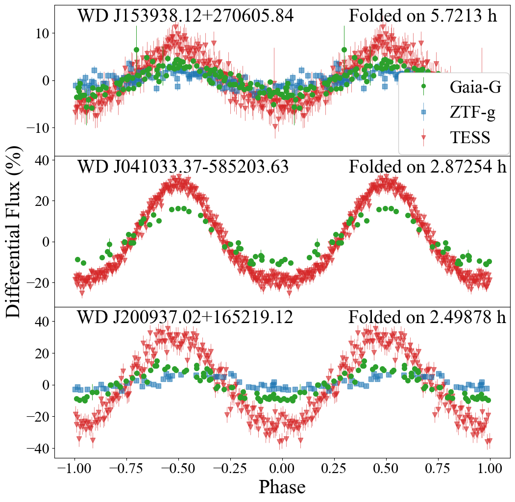
Figure 2: Phase-folded light curves of three representative variable white dwarfs from binarity, revealing orbital periods of 5.725 hr, 2.873 hr, and 2.500 hr, respectively. All folded light curves (ZTF $g$ in blue, Gaia $G$ in green, and TESS photometry in red) are phased to the same ephemeris. ZTF $g$ and TESS data are grouped into 151 bins for each light curve. The larger amplitudes at redder wavelengths in these systems indicates they are all likely reflection-effect binaries of a cool main-sequence star reprocessing flux from a nearby hot white dwarf.

Three representative examples of variable binaries are shown in Figure 2. The first object (WD J153938.12$+$270605.84, $G$ = 16.6 mag) is a known DA+dM system with an orbital period of $5.72120\pm 0.00087$ hr measured from the Palomar Transient Factory (PTF, Kao et al., 2016). We measure from Gaia DR3 photometry only $P_{\mathrm{orb}}=5.7213\pm 0.0053$ hr, agreeing with the PTF measurement to within our estimated uncertainty. The second object (WD J041033.37$-$585203.63, $G$ = 17.6 mag) is a newly discovered binary system with a sinusiodal pattern in both the Gaia $G$ and TESS bands with a Gaia $G$ band period of $2.87254\pm 0.00054$ hr. The higher amplitude from the redder TESS data is indicative of flux reprocessing from a reflection-effect binary, though no spectroscopy exists for this target. Finally, WD J200937.02$+$165219.12 ($G$ = 16.8 mag) is also likely a new reflection-effect binary with an orbital period of $2.49878\pm 0.00086$ hr.

The shortest-period, likely detached new binary in our sample is WD J123955.40$+$834707.51 ($G$ = 20.0 mag), which shows significant variability in ZTF at $0.95661\pm 0.00015$ hr that is also seen in the Gaia $G$-band light curve at an amplitude exceeding 40%. No spectroscopy exists of this target, which has a position in the Gaia CMD consistent with a 7020 K, 0.27 $M_{\odot}$ white dwarf, suggesting it might be a new WD+WD binary containing at least one ELM white dwarf (e.g., Brown et al. 2022).

4.2 Periodicities in Known Cataclysmic Variables

There are also likely some binaries that are not detached in our sample. CVs are a class of accreting white dwarf binaries, and are often eruptive variables that show large brightening events from dwarf novae and other outbursts (Szkody et al., 2020, 2021). We have not intended to search for new CVs among the 1333 high-confidence white dwarfs, which has been the focus of previous work on Gaia light curves using eruptions and outbursts (e.g., Gaia Collaboration et al. 2019). However, we have identified coherent periods in three objects classified as CVs in the literature.

WD J083843.35$-$282701.14 ($G$ = 17.6 mag) is a known CV (Halpern et al., 2017; Rea et al., 2017) for which we find a new potential period of variability of $16.109\pm 0.029$ hr. This period differs slightly from the approximately 15-hr period of flux variability interpreted as the beat period between the orbital and spin periods (Rea et al., 2017), as well as the $14.7\pm 1.2$ hr period of X-ray modulations observed by Halpern et al. (2017). WD J031413.25$-$223542.92 ($G$ = 18.2 mag) was studied by Warner (1980) and Bond et al. (1979). The Gaia DR3 data show a significant periodicity at $1.34947\pm 0.00017$ hr, which is in close agreement with both studies.

Finally, WD J130017.86$-$325805.23 ($G$ = 20.3 mag), is a CV candidate that has undergone at least two measured outbursts detected in CRTS (Drake et al., 2014). We lack TESS or ZTF coverage for this faint southern object, but all three Gaia band-passes have their highest periodogram peak at 2171.36 s (36.2 min). The amplitude of the signal exceeds 80% in all Gaia band-passes. Such large-amplitude periodic variations are not commonly observed as spurious signals in Gaia DR3 at such short periods (Holl et al., 2023), though we cannot independently rule out an instrumental origin for this 36.2-min variability. We strongly encourage follow-up of this faint southern target.

4.3 Eclipsing White Dwarf Binaries

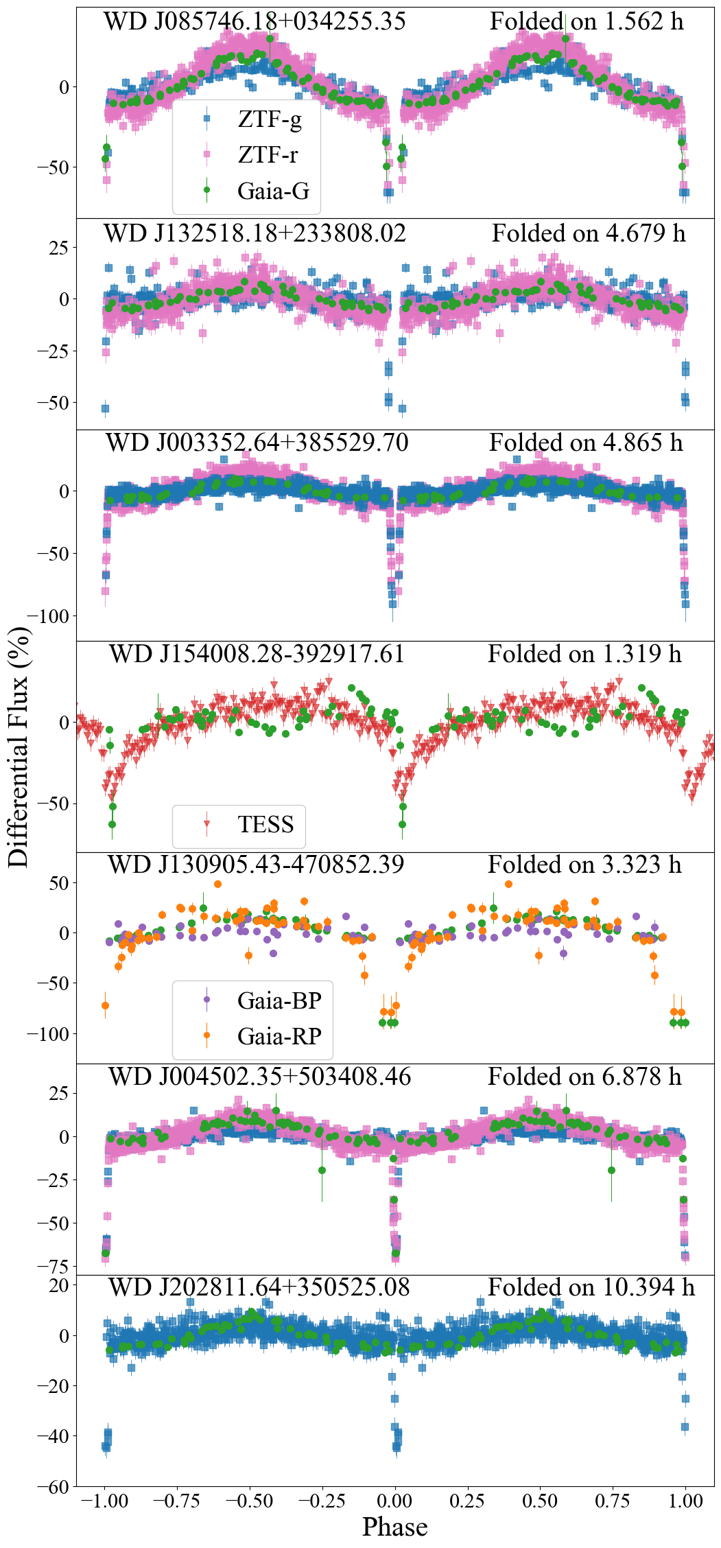
Figure 3: Following the same convention as Figure 2, we show phase-folded light curves of seven eclipsing binaries detected from their Gaia DR3 light curves. In this figure, ZTF and Gaia data are not binned, but TESS data are grouped into 251 bins. The first three systems are previously published eclipsing binaries containing a white dwarf (Drake et al., 2010; Parsons et al., 2015; Kosakowski et al., 2022). Four systems are newly discovered eclipsing binaries containing a white dwarf, including a new 1.3-hr eclipsing CV (WD J154008.28$-$392917.61, further detailed in Section 4.3.1 and Figure 4). With only sparse Gaia DR3 data, we do not claim to confirm binarity in WD J154008.28$-$392917.61, but include it as an interesting candidate.

Eclipsing binaries often display near-total flux dropouts in randomly sampled light curves (Parsons et al., 2013), as the fainter companion passes in front of the brighter member. These eclipses should occur at exactly the same phase in a folded light curve, manifesting as stable, repeated photometric variability. The seven known and likely eclipsing systems are shown in Figure 3.

The top panels in Figure 3 detail three previously known eclipsing white dwarf binaries, in order of orbital period. WD J085746.18$+$034255.35 ($G$ = 18.3 mag) is a known eclipsing WD+dM with a measured orbital period of 1.562317 hr by the Catalina Sky Survey (CSS, Parsons et al. 2015), which is consistent with our measurement from Gaia DR3 photometry of $1.562316(17)$ hr. This object shows both ZTF and Gaia dropouts, notable since the Gaia DR3 light curves have a reasonably aggressive outlier rejection (Eyer et al., 2023). WD J132518.18$+$233808.02 ($G$ = 18.2 mag) is also a known eclipsing DA+dM binary with an orbital period of 4.679 hr measured by CSS (Drake et al., 2010; Parsons et al., 2015) consistent with our measurement from Gaia DR3 photometry of $4.67901(39)$ hr. The lack of in-eclipse data from Gaia is likely related to outlier rejection of the Gaia photometry. WD J003352.64$+$385529.70 ($G$ = 18.3 mag) was identified by Kosakowski et al. (2022) to have a strong 4.86-hr signal in ZTF, and has all the hallmarks of a WD+dM eclipsing binary, especially featuring ZTF dropouts in both the $g$- and $r$-bands when folded on a period of $4.86465(31)$ hr. These dropouts align in phase space and show a decrease in amplitude of nearly 100%.

Our analysis identifies four new candidate eclipsing binaries. Most compact is WD J154008.28$-$392917.61, showing multiple low Gaia points when folded on the TESS-determined period of $1.319(13)$ hr. We detail follow-up observations of this source in Section 4.3.1 and Figure 4.

WD J130905.43$-$470852.39 ($G$ = 18.3 mag) may be an eclipsing binary, having only Gaia light curves to analyze. When folded on a period of $3.32265(44)$ hr, the source shows dropouts in both the $G$ and $G_{\mathrm{RP}}$ bands with small uncertainties leading us to believe that these are genuine eclipses. Photometric fits to the Gaia CMD suggest this system has an extremely low-mass ($<$0.16 $M_{\odot}$), 11040 K white dwarf with a high probability of being a white dwarf ($P_{\rm WD}=0.91$, Gentile Fusillo et al. 2021). With only sparse Gaia DR3 data and possibly long transit durations, we cannot confirm this system as eclipsing yet, but encourage further follow-up.

We are far more confident in the fidelity of the final two systems shown in Figure 3. WD J004502.35$+$503408.46 ($G$ = 17.6 mag) is over-luminous to the isolated white dwarf position in the Gaia CMD (suggesting binarity) and features ZTF and Gaia dropouts suggesting an orbital period of $6.87794(72)$ hr. WD J202811.64$+$350525.08 ($G$ = 17.9 mag), is also over-luminous and features ZTF dropouts when folded on a period of $10.3937(17)$ hr. There is also a strong Gaia-$G$ sinusiodal pattern that aligns with the ZTF data with a minimum in the time of transit.

4.3.1 Follow-Up of a New Eclipsing CV

We obtained follow-up time-series photometry and spectroscopy for our most compact new eclipsing system (WD J154008.28$-$392917.61), located in the southern hemisphere ($G$ = 17.3 mag).

We obtained high-speed time-series photometry using the ULTRACAM instrument (Dhillon et al., 2007) mounted on the 3.6-meter New Technology Telescope (NTT) telescope at the La Silla Observatory in Chile. This camera obtains simultaneous three-channel photometry with frame-transfer detectors; we used high-throughput Super-SDSS $u_{s}g_{s}r_{s}$ filters (Dhillon et al., 2021). We observed WD J154008.28$-$392917.61 over two consecutive nights, analysing here only the SDSS-$g_{s}$ data. We collected 9.0-s exposures on UT date 2023 March 16 with an average seeing of 0.8 arcsec. We collected 4.5-s exposures on UT date 2023 Mar 17 with an average seeing of 0.7 arcsec. All ULTRACAM data were bias-subtracted and flat-field corrected using the HiPERCAM pipeline.

We also obtained follow-up spectroscopy of this system using the Goodman spectrograph (Clemens et al., 2004) mounted on the 4.1-meter SOAR Telescope in Chile. We collected eleven $10$ min spectra using the 400-line grating with a 1-arcsec slit and the M1 grating setup on UT date 2023 May 24, yielding a resolution of roughly 4.4 Å. We extracted the data using the pypeit data reduction pipeline (Prochaska et al., 2020), and flux calibrated using the standard star EG 274.

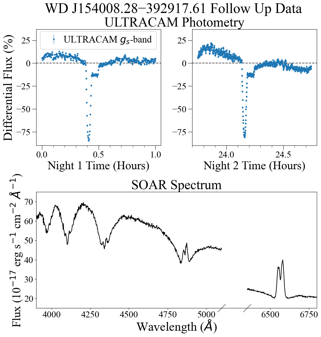
Figure 4: Follow up data for WD J154008.28$-$392917.61 reveals deep primary eclipses in the two top panels. Follow-up spectroscopy (note the broken x-axis) confirms this is a 68.365-min CV, likely descending from a previously detached white dwarf + brown dwarf post-common-envelope binary (e.g., Littlefair et al. 2007).

We captured two primary eclipses with ULTRACAM, shown in the top two panels of Figure 4. Fitting the mid-time of the eclipses with a Gaussian bounded by when the flux decreases below $-$20%, we find that the primary eclipses occur at BJD_TDB = 2460019.8887179(17) and 2460020.8778468(11), separated by 18 cycles of our TESS-determined main periodicity of $1.319(13)$ hr. There is considerable out-of-transit variability, including an extended feature from a bright spot on the white dwarf, seen in many eclipsing CVs (e.g., Savoury et al. 2011; McAllister et al. 2019).

Our coadded spectrum in the bottom panel of Figure 4 confirms this is an accreting white dwarf binary. Broad Balmer-line absorption from the white dwarf is visible, along with strong emission features from accretion, especially dominant at H$\alpha$. Our spectrum is not high-enough resolution to attempt a radial-velocity fit. We do not observe Zeeman splitting at the Balmer lines, though our limits are weak given the strong emission in the line cores.

A purported orbital period of 68.365 min is well below the CV period minimum of roughly 80 min, after which convective donor stars expand on further mass loss (Patterson, 1984; Knigge et al., 2011; Kalomeni et al., 2016; McAllister et al., 2019). However, the full photometric phase coverage from TESS shown in Figure 3 reveals this is the correct period of recurrent variability. This makes WD J154008.28$-$392917.61 among the shortest-period CVs known, similar to the 66.61-min CV SDSS J150722.30$+$523039.8 (Littlefair et al., 2007). These ultracompact CVs are likely descended from a previously detached white dwarf + brown dwarf binary. It is also possible the system descended from a low-metallicity, significantly evolved donor (Uthas et al., 2011).

4.4 Magnetic Spotted White Dwarfs

Spotted white dwarfs are difficult to distinguish from reflection-effect binaries like those discussed in Section 4.1. When spectroscopy is not available, we classify all objects with apparently mono-periodic variability and photometrically determined (Gentile Fusillo et al., 2021) masses $>$0.525 $M_{\odot}$ and temperatures $<$$31{,}000$ K as isolated white dwarfs with rotational modulation from magnetic spots.

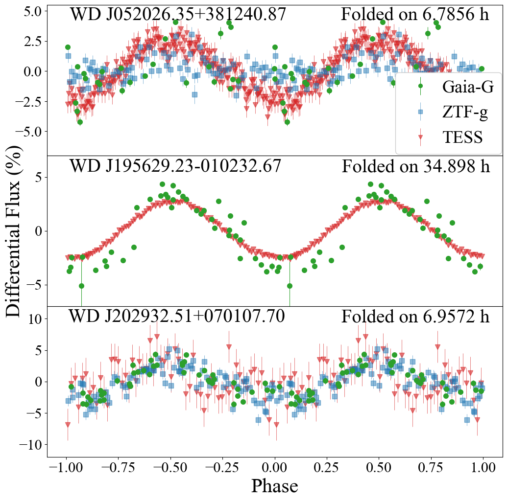
Figure 5: Following the same convention as Figure 2, we show phase-folded light curves of three magnetic spotted white dwarfs. ZTF-$g$ and TESS data are grouped into 151 phase bins, whereas the Gaia data are not binned.

The period of the spot-induced modulations corresponds to the rotational period at the star’s surface (e.g., Brinkworth et al. 2013; Kilic et al. 2015; Hoard et al. 2018). We recover the periods of eight previously known spotted white dwarfs from the Gaia DR3 light curves independently, and identify 17 new likely spotted white dwarfs. The majority of the newly identified spotted white dwarfs (12/17) have effective temperatures between $6500-10{,}000$ K, placing them inside the range of known DAHe strongly magnetic white dwarfs with Balmer-line emission (Greenstein & McCarthy, 1985; Reding et al., 2020; Gänsicke et al., 2020; Walters et al., 2021; Reding et al., 2023; Manser et al., 2023), motivating future time-resolved spectroscopic follow-up. Our sample contains several known DAHe (see Table Measuring White Dwarf Variability from Sparsely Sampled Gaia DR3 Multi-Epoch Photometry). WD J083531.17$+$533230.91 ($G$ = 18.2 mag) is the only other spectroscopically confirmed strongly magnetic white dwarf in our sample, and appears to have a 2.16-hr period.

Examples of three spotted white dwarfs are shown in Figure 5. The top object WD J052026.35$+$381240.87 ($G$ = 15.4) is a spectroscopically confirmed white dwarf from LAMOST claimed to be a DBA (Kong et al., 2019) but is likely a DAH; Gaia DR3 photometry shows it is likely rotating at $6.7856\pm 0.0046$ hr. The second object (WD J195629.23$-$010232.67, $G$ = 13.6 mag) has been known to be spotted (the white dwarf is highly magnetic with a complex field structure, shown in Maxted et al. 2000). We observe clear sinusoidal variability in the $G$ data with a period of $34.898\pm 0.074$ hr, in close agreement with the literature value from Brinkworth et al. (2005). The final object is WD J202932.51$+$070107.70 ($G$ = 16.6 mag), a known DO white dwarf (Dreizler et al., 1995). This white dwarf was observed to have a ZTF $g$ photometric variability period of $6.97882\pm 0.00012$ hr from Reindl et al. (2021), which is close to our LLS fit to the Gaia-$G$ data of $6.9572\pm 0.0022$ hr. It is likely that the ZTF or Gaia data has selected an incorrect alias due to gaps in the data.

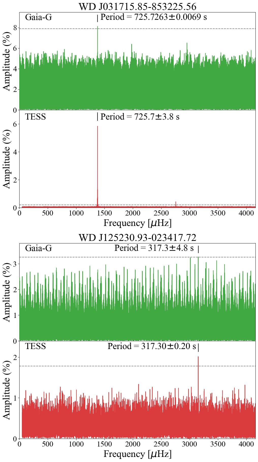
Figure 6: Lomb-Scargle periodograms showing two rapidly rotating spotted white dwarfs recovered in sparsely sampled Gaia DR3 light curves. At top is WD J031715.85$-$853225.56 (Ferrario et al., 1997); the 725 s variability period has a $<$0.1% false-alarm probability in the Gaia $G$ light curve. At bottom is WD J125230.93$-$023417.72, which has a 0.1% false-alarm probability, with the highest peak in the periodogram at exactly the same period, within the uncertainties, as the known variability discovered by Reding et al. (2020).

Figure 6 demonstrates Gaia DR3 light curves are able to recover the variability in two of the shortest-period spotted white dwarfs known. The top panel details WD J031715.85$-$853225.56 ($G$ = 14.8 mag), a well-studied, rapidly rotating, high-field magnetic white dwarf (Ferrario et al., 1997). The Gaia $G$ peak occurs at the same period as the TESS data, to within the uncertainties of the LLS fits. The light curve from Gaia is sparsely sampled, with visits separated by $32.5\pm 8.8$ d, where 8.8 d is the standard deviation of the time between visits. False-alarm probability lines for periodograms are estimated by holding the time sampling the same but randomly shuffling the fluxes with replacement 10,000 times, in an attempt to quantify the probability that the amplitude of a peak can be generated by pure noise (e.g., Greiss et al. 2014; VanderPlas 2018). For WD J031715.85$-$853225.56 at the top of Figure 6, none of our bootstrapped periodograms have a peak as high as the observed Gaia $G$ periodogram, yielding a false-alarm probability of $<$0.1%.

In the bottom panel of Figure 6 we show Gaia and TESS peaks measured for the strongly magnetic, emission-line (DAHe) white dwarf WD J125230.93$-$023417.72 ($G$ = 17.5 mag, Reding et al. 2020). While not statistically significant, the highest peak in the Gaia periodogram occurs at the known dominant period of 317.278 s (which is the first harmonic the 634.56-s rotation period, see Farihi et al. 2023). We bootstrap a false-alarm probability of 0.1% for this peak.

Aside from these two previously known spotted white dwarfs, we recover the literature periods for six other known spots. Two are known emission-line DAs: the 36.3-min DAHe system WD J003512.88$-$122508.84 (Reding et al., 2023) and the 2.29-hr, non-magnetic DAe white dwarf WD J041246.84$+$754942.26 (Tremblay et al., 2020; Elms et al., 2023). We recover two cooler white dwarfs with spots: the 0.72-hr WD J053432.93$+$770757.40 (Guidry et al., 2021) and the 1.44-d WD J195629.23$-$010232.67 shown in Figure 5. We also recover two much hotter spotted stars discussed at the end of Section 3, the 6.98-hr WD J202932.51$+$070107.70 (Reindl et al., 2021) and the 3.45-d WD J095125.94$+$530930.72 (Werner et al., 2019).

The shortest-period new spotted white dwarf in our sample is WD J115033.35$-$063618.07 ($G$ = 16.4 mag). This spotted white dwarf features a highest peak in the $G$ light curve matching the TESS-significant peak at $884.0679\pm 0.0094$ s. Spectropolarimetry puts a 3$\sigma$ upper limit on the magnetic field of LP 673-41 of $<$6 kG (Kawka & Vennes, 2012), raising questions about the origin of the spot on this 8600 K white dwarf. The longest period spot appears on WD J124740.10$+$303007.41 ($G$ = 17.9 mag), with a highest peak in the periodogram at 9.487 d in both its Gaia and ZTF light curves.

4.5 Pulsating White Dwarfs

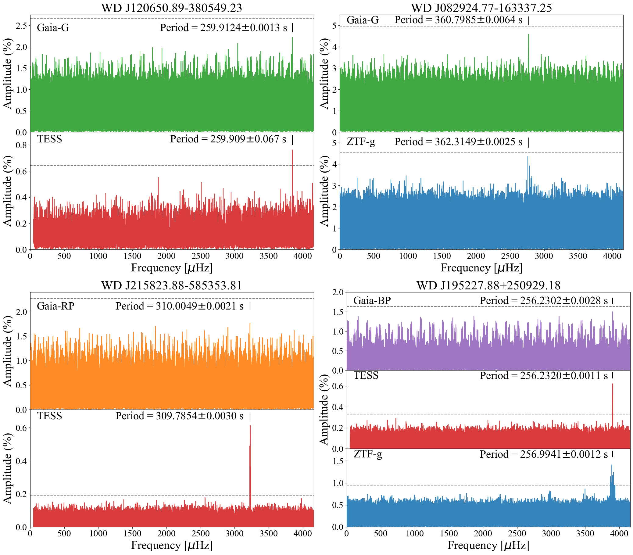
Figure 7: Panels of periodograms for the four objects we classify as Gaia-detected pulsating white dwarfs, all with periods $<$400 s. The photometric bands in these figures are $G$, $G_{\mathrm{BP}}$, $G_{\mathrm{RP}}$, $g$, $r$, $T$ (Gaia G, BP, and RP bands, ZTF g and r bands, and the TESS photometry band, respectively). A bootstrapped 99.9% confidence lines is shown as a horizontal dashed line in gray (see description in Section 4.4). The false-alarm probabilities of all four Gaia peaks are all between 2.5% and 28.9% (see Table Measuring White Dwarf Variability from Sparsely Sampled Gaia DR3 Multi-Epoch Photometry).

Pulsating white dwarfs are variable due to non-radial pulsations, with periods typically ranging from $100-1500$ s, amplitudes up to several percent, and usually multiple, non-harmonically related periods present at the same time (Fontaine & Brassard, 2008; Winget & Kepler, 2008b). DA white dwarfs are unstable to pulsations in a narrow temperature range between roughly $13{,}500-10{,}500$ K (Hermes et al., 2017c). These hydrogen-atmosphere pulsators are commonly known as ZZ Cetis and DAVs.

From Gaia DR3 photometry alone we are able to independently identify the periods for two new candidate pulsating white dwarfs and confirm the periods of two known DAVs. All objects lie within the empirical DAV instability strip in the Gaia color-magnitude diagram (Figure 1), and their Lomb-Scargle periodograms are shown in Figure 7. As with our spotted white dwarfs in Figure 5, we bootstrap false-alarm probabilities to assess the significance of a peak in the periodogram and quantify the likelihood a peak cannot arise from noise alone. The significance lines in Figure 7 are the 99.9% confidence line ($<$0.1% false alarm); false-alarm probabilities for all objects in this manuscript are listed in Table Measuring White Dwarf Variability from Sparsely Sampled Gaia DR3 Multi-Epoch Photometry. While none of our pulsating white dwarfs have formally significant peaks, the chance that the highest peak in the periodogram exactly matches significant peaks in an independent ZTF or TESS dataset is exceptionally low; our periodograms all have step sizes of 0.01 $\mu$Hz and run beyond 4000 $\mu$Hz, giving hundreds of thousands of trial frequencies. In three of the four cases in Figure 7, the false-alarm probability is $<$10%.

We find WD J120650.89 $-$380549.23 ($G$ = 15.7 mag) is a new pulsating WD with a pulsation period at $259.9127\pm 0.0013$ s in $G$ with a 8.1% false-alarm probability that is also significantly detected in TESS. WD J215823.88-585353.81 ($G$ = 15.8 mag) is a known DAV with multiple detected modes from rotational splittings revealed by TESS at 310.27 s, 309.79 s, and 309.31 s (Romero et al., 2022). The highest peak in the $G_{\mathrm{RP}}$ periodogram is consistent with this pulsational variability, at a period of $310.0049\pm 0.0021$ s, though this peak has a marginal 28.9% false-alarm probability. WD J082924.77$-$163337.25 ($G$ = 17.6 mag) was identified as a variable white dwarf in Guidry et al. (2021). We detect variability consistent with pulsations in both the Gaia-$G$ and ZTF-$g$ light curves at $359.0045\pm 0.0025$ s, with just a 2.5% false-alarm probability. Finally, WD J195227.88$+$250929.18 ($G$ = 15.1 mag), is a known DAV with a dominant pulsation period of 256.2 s (Kepler, 1984; Fontaine et al., 1980). Our analysis agrees closely with a peak in $G_{\mathrm{BP}}$ at $255.999\pm 0.001$ s and a 3.7% false-alarm probability of matching peaks in ZTF and TESS.

The four white dwarfs with likely pulsations detected in their Gaia light curves all have periods $<$400 s; longer-period modes are likely unstable over long baselines (Hermes et al., 2017c), suggesting longer-period modes will be hard to detect from Gaia data independently. However, pulsating white dwarfs appear to be the most numerous white dwarfs flagged as variable in Gaia DR3. There is an overdensity of points in Figure 1 near the DAV instability strip relative to the 200-pc sample of white dwarfs in the background. In fact, of the 883 candidate white dwarfs that are flagged as photometrically variable in Gaia DR3 with $P_{\mathrm{W}D}>0.98$ and masses $>$0.45 $M_{\odot}$ from Gentile Fusillo et al. (2021), nearly half (422) have effective temperatures near the DAV instability strip boundaries ($13{,}500>$${T}_{\mathrm{eff}}$$>10{,}500$ K). Literature searches of this sample reveal at least 50 are already-known DAVs, and at least 120 that can be photometrically confirmed with TESS, ZTF or ASAS-SN data; this analysis will be presented in a future publication.

5 Gaia-Detected Periods

We use Gaia DR3 epoch photometry, which includes photometric time series data in the $G$-, $G_{\mathrm{BP}}$-, and $G_{\mathrm{RP}}$- bands (Eyer et al., 2023). Each time-series data point is a so-called field-of-view transit, after an object has passed through nine consecutive CCD observations, each separated by 4.85 s (Roelens et al., 2018). As the Gaia spacecraft spins, objects will then be re-observed at a cadence separated by 1 hr 46 min (Roelens et al., 2017). The time sampling after this revisit is considerably longer, and different for each source, set by the Gaia scanning law (e.g., Boubert et al. 2021).

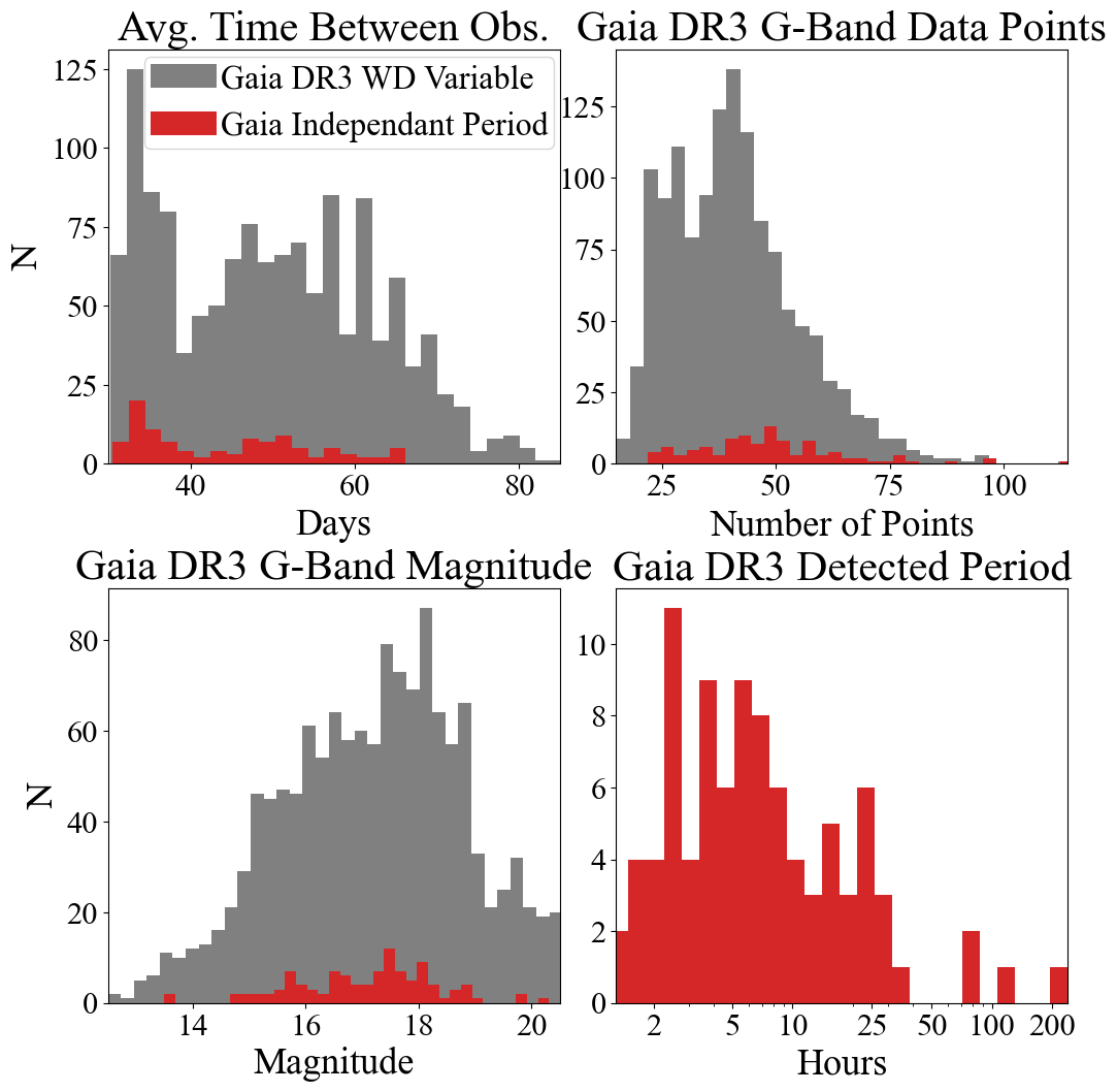
Figure 8: Top left histogram shows the average time between Gaia DR3 observations (ignoring the 1 hr 46 min revisit) for the full sample of 1333 candidate white dwarfs flagged as variable in gray, inset in red by the 105 candidate white dwarfs in this manuscript where their variability period can be determined by Gaia independently. The top right panel shows the number of points in each $G$ light curve, and the bottom left panel shows the $G$ magnitude distribution of both samples. The bottom right panel shows the distribution of the 105 periods for objects detected by Gaia independently (note that the x-axis is log scale). Although we are slightly more sensitive to objects with more frequent visits, our sample of 105 sources covers most of this parameter space.

We analyze the revisit cadence of these observations by creating a histogram of the average time between each observation, shown in Figure 8. We ignore the revisit timescale of 1 hr 46 min (set by the 6-hr spin period of Gaia, as discussed in de Bruijne 2012) by excluding time between observations of less than 0.3 days, and find an average time of $49.7\pm 12.5$ d between observations for the full sample of 1333 objects (the uncertainty is set by the standard deviation of these revisit times). Of the 105 objects where we can measure variability from the Gaia light curves independently, the average revisit time is $44.2\pm 10.3$ d. Our subset of 105 objects has slightly less time between observations, only a few more Gaia-G data points (with an average number of points of $49\pm 17$ compared to $41\pm 14$ for the full sample), and is slightly brighter (with an average magnitude of $G=17.0\pm 1.2$ mag compared to $G=17.2\pm 1.6$ mag for the full sample). The distributions in Figure 8 show we are not heavily biased towards objects with frequent revisits set by the Gaia scanning law. The average and standard deviation in the revisit times between FoV transits for each object is included in Table Measuring White Dwarf Variability from Sparsely Sampled Gaia DR3 Multi-Epoch Photometry. Among the 72 of 105 objects with ZTF data, the average object has 393 ZTF visits, which is completely consistent with the typical sky coverage of the average fields in ZTF DR12.

We also analyze short-period variability in the Gaia DR3 light curves, which is measured as the object moves from one CCD to the next every 4.85 s (e.g., Roelens et al. 2018). Included in DR3 are per-CCD least-squares fits listed as “Frequency” for objects flagged as vari_short_timescale, for select objects with candidate variability periods shorter than 0.5 d. The inverse of the vari_short_timescale frequency is listed in Table Measuring White Dwarf Variability from Sparsely Sampled Gaia DR3 Multi-Epoch Photometry as $P_{\rm G,S}$, and we check each period generated by our LLS fit ($P_{\rm G,DR3}$ in Table Measuring White Dwarf Variability from Sparsely Sampled Gaia DR3 Multi-Epoch Photometry) against $P_{\rm G,S}$. In our final 105 object sample, 65 objects are flagged in Gaia DR3 as short-timescale sources, and 55 of these 65 (85%) have $P_{\rm G,S}$ that matches $P_{\rm G,DR3}$ to within 3% (after which the agreement is never better than 22%).

We compare the Gaia DR3 short-timescale analysis against our LLS fits by object type. We find that of our 72 binary objects, 48 of 53 (91%) with vari_short_timescale data have $P_{\rm G,S}$ that matches our determinations of $P_{\rm G,DR3}$, and of the spotted white dwarfs, 5 of 7 with short-timescale analysis match. For all variable types, the Gaia DR3 short-timescale analysis returns 55/60 (92%) matches for objects with vari_short_timescale between 0.278 and 2.78 hours, and routinely does poorly for periods longer than 3 hr.

We also attempt to assess the reliability of the Gaia variability identifier (Eyer et al., 2023). Gaia uses a machine learning algorithm trained on non-variable objects and then tested against training sets (built from various published catalogues of variable stars) to confirm how effectively this algorithm can identify variable objects. Objects are categorized as variable when there is a large value for the ratio of the difference in magnitude from the average for that object to the interquartile range of the magnitude. These objects are then passed through one of two paths in the machine learning process to be sorted into a specific Gaia “class,” discussed in depth in Rimoldini et al. (2023). This Gaia class is listed in Table Measuring White Dwarf Variability from Sparsely Sampled Gaia DR3 Multi-Epoch Photometry.

We find that this “class” is not generally useful, as most are simply “WD.” There is one case where this class correctly identifies a known CV (WD J130017.86$-$325805.23). The Gaia “class” also marks two objects as “S” or stars with short-timescale variability: WD J083843.35$-$282701.14 (a known CV with $P_{\rm G,S}$ that matches $P_{\rm G,DR3}$ at $16.109\pm 0.029$ hr) and WD J233923.79$-$485350.19 (a likely new binary system with $P_{\rm G,S}$ that matches $P_{\rm G,DR3}$ at $2.52962\pm 0.00075$ hr). The new eclipsing CV WD J154008.28$-$392917.61 also has a Gaia “class” of CV.

Finally, we note that Gaia epoch photometry may contain spurious periodicities due to scan-angle-dependent signals, especially in marginally resolved, fixed-orientation pairs of stars separated by $<$0.5 arcsec (Holl et al., 2023). Although previous work has only explored signals up to 10 days, and most signals determined here are below that, we investigate the likelihood that any of our detections are spurious.

All 1333 white dwarf candidates in our sample have information in the vari_spurious_signals table from Holl et al. (2023), including important metrics that can reveal close binarity, the Spearman rank correlation coefficient with corrected flux excess factor ($r_{\rm exf,G}$) and the Image Parameter Determination model ($r_{\rm ipd,G}$). Only three white dwarfs have both $r_{\rm exf,G}$ and $r_{\rm ipd,G}$ values $>$0.8 (WD J020426.03$+$571026.62, WD J031047.57$-$100153.85, and WD J100643.74$-$221757.86), none of which are included in our subset of 105 white dwarfs with variability measured independently from Gaia. In our subset of 105 objects, only one has $r_{\rm ipd,G}>0.6$ and that is WD J003512.88$-$122508.84, which has confirmed variability from TESS (Reding et al., 2023). We conclude that contamination from spurious Gaia scanning-law-dependent periods is unlikely in our sample of white dwarfs.

6 Discussion & Conclusions

We analyze 105 white dwarf candidates for which Gaia is capable of detecting accurate periods from DR3 photometry. These periods of variability range from 9.5 d to as short as 256.2 s (roughly 4 min), including seven objects with periods shorter than 1000 s. We obtained this result by comparing Gaia multi-band photometry to data from ZTF and TESS to identify significant periods within the Gaia data. Analysis of the Gaia photometry resulted in the discovery of new pulsating, spotted and binary white dwarfs. This includes a new 68.4-min eclipsing cataclysmic variable, which has a period well below the CV period minimum of roughly 80 min (Knigge et al., 2011) and is one of the shortest-period CVs known.

Our overall analysis demonstrates that Gaia epoch photometry is precise enough to detect short-term, low-amplitude periods even when observations are sparsely sampled. The absolute median amplitude of the photometric variability we confirm from Gaia independently is $1.4\%$, with an average period of roughly 12 hr. This is notable compared to the distribution of time between observations, which is on average roughly 44 d. We find that overall, the 105 variables that are significant in Gaia are slightly brighter and sampled more often than the full sample of 1333 objects, but the distributions of magnitudes or number of points are not significantly biased in either parameter space, as shown in Figure 8.

The likelihood that the highest peak in two independent periodograms match is small, given that there are more than $10^{5}$ frequency elements in each periodogram. This is the basis for which we claim Gaia has detected a periodicity. Still, we have bootstrapped estimates that a peak in the periodogram can be caused by noise alone and find that 33/105 objects have significant peaks in their Gaia light curves, with a $<$0.1% false-alarm probability. Nearly half the sample, 50/105, have peaks with a false alarm $<$1%. Only three have $>$35%, but all 105 have Gaia peaks with a $<$41% false-alarm probability (Table Measuring White Dwarf Variability from Sparsely Sampled Gaia DR3 Multi-Epoch Photometry details this value for all objects in our sample). Our work provides an empirically determined set of cutoffs for which variability in a Gaia DR3 light curve is likely to be genuine, and it also represents a useful value for future analysis of sparsely sampled, high-precision photometry from large surveys like the Vera C. Rubin Observatory and its Legacy Survey of Space and Time (LSST; Ivezić et al. 2019), as well as the Nancy Grace Roman Space Telescope (Akeson et al., 2019).

Previous spectroscopy exists for only 36 of the 105 objects discussed in this paper, so follow up is encouraged for most of these sources. There are many objects of interest that would expand sample sizes of rare object types. Some notable examples include WD J123955.40$+$834707.51 ($G$ = 20.0 mag), which may be a new WD+WD binary containing an ELM white dwarf, and WD J130017.86$-$325805.23 ($G$ = 20.3 mag) which is a candidate CV with recorded outbursts (Drake et al., 2014) but shows a dominant photometric period of 36.2 min closer to the orbital period of AM CVn binaries (see Section 4.1). There are also multiple candidate eclipsing binaries discussed in Section 4.3. Finally, one of the shortest-period new spotted white dwarfs we discovered here (WD J115033.35$-$063618.07) appears to have an 884.73-s spin period but a $<$6 kG magnetic field, raising questions about the origin of its fast rotation (see Section 4.4).

As Gaia continues to scan the sky, the methods discussed in this paper provide a foundation for analyzing short-period variables within even longer-baseline data. Verifying that Gaia data independently can be used to detect short periods will allow future work on sources with no additional spectroscopic or photometric information. Increasing the numbers of rare variable stellar remnants, especially those in short-period binaries or with magnetic spots, will help constrain their space density and formation channels.

7 acknowledgements

The authors thank the anonymous referee for a very useful report, as well as fruitful discussions with Stu Littlefair. Support for this work was in part provided by NASA TESS Cycle 2 Grant 80NSSC20K0592 and Cycle 4 grant 80NSSC22K0737, as well as the National Science Foundation under grant No. NSF PHY-1748958, as portions of this project were completed at the KITP Program “White Dwarfs as Probes of the Evolution of Planets, Stars, the Milky Way and the Expanding Universe.”

The authors acknowledge the European Southern Observatory program 110.23UU.001, as well as the Transiting Exoplanet Survey Satellite (TESS), the Zwicky Transiting Facility (ZTF), the All-Sky Automated Survey for Supernovae (ASAS-SN), and the Asteroid Terrestrial-impact Last Alert System (ATLAS) for the public release of all-sky photometry data for many of these objects. This work has also made use of data from the European Space Agency (ESA) mission Gaia (https://www.cosmos.esa.int/gaia), processed by the Gaia Data Processing and Analysis Consortium (DPAC, https://www.cosmos.esa.int/web/gaia/dpac/consortium). Funding for the DPAC has been provided by national institutions, in particular the institutions participating in the Gaia Multilateral Agreement.

This research is also based on observations obtained at the Southern Astrophysical Research (SOAR) telescope, which is a joint project of the Ministério da Ciência, Tecnologia e Inovações (MCTI/LNA) do Brasil, the US National Science Foundation’s NOIRLab, the University of North Carolina at Chapel Hill (UNC), and Michigan State University (MSU).

=16mm

Table 2: Literature information for the 105 white dwarfs in this study with significant variability measured from their Gaia DR3 light curve.

Class	Gaia Source ID	WD J Name†	RA	DEC	$G$	$P_{\rm WD}$†	${T}_{\mathrm{eff}}$†	Mass†	Sp. Type	Dist.	Class‡	Score‡	$N_{\rm G}$‡	$N_{\rm g}$∗∗	Skew‡	IQR‡	$N_{\rm G,S}$∗	Abbe∗	$P_{\rm G,S}$∗	$P_{\rm lit}$	Ref.
(This Work)	(DR3)		(J2016)	(J2016)	[mag]		[K]	[$M_{\odot}$]		[pc]					($G$)	($G$)			[hr]	[hr]
Likely Binary	2780903539324180736	WD J003213.13+160434.78	8.054739	16.076395	15.7	0.982			DO	415.3	WD	0.6	50	68.0	0.755	0.036	50.0	0.836	21.7869583		1
Likely Binary	2317319612801004416	WD J003449.86-312952.69	8.707866	-31.497956	16.1	0.882	25410.0	0.24	DA	431.1			39		-0.416	0.133	39.0	0.822	2.3167499		2
Likely Binary	522432163970498048	WD J011053.06+604831.03	17.721109	60.808565	17.0	0.949	14770.0	0.2		301.7			58	491.0	-0.088	0.068	58.0	0.872	8.3619614
Likely Binary	323342459647016448	WD J012828.99+385436.63	22.12078	38.910093	15.9	0.998	38310.0	0.54	DA	236.1	WD	0.651	30	375.0	-0.396	0.025					3
Likely Binary	2478893842934875136	WD J013148.02-055900.14	22.950116	-5.983399	17.3	0.939	96630.0	0.63		930.9	WD	0.465	44	329.0	-0.49	0.041
Likely Binary	459237630076876672	WD J022704.24+591502.04	36.768226	59.25064	15.9	0.988	7360.0	0.51	DA	37.7	WD	0.52	48	420.0	0.282	0.029					4
Likely Binary	4846154678323893248	WD J032205.10-472106.46	50.521313	-47.351787	17.3	0.978				970.5	WD	0.501	48		0.465	0.121
Likely Binary	117770030481927936	WD J032803.02+265151.65	52.012578	26.864324	18.2	0.98				656.2	WD	1.0	27	426.0	-0.095	0.16
Likely Binary	235184643828418688	WD J032902.63+390340.87	52.260969	39.061346	18.6	0.973				876.2	WD	0.5	41	251.0	-0.841	0.082	42.0	0.984	4.0387314
Likely Binary	5090605830056251776	WD J035814.52-213813.74	59.560498	-21.637194	17.8	0.938	24810.0	0.24		802.3			76	242.0	-0.302	0.147	77.0	0.924	1.7951253
Likely Binary	4681729620697295360	WD J041033.37-585203.63	62.639044	-58.867634	17.6	0.94	15430.0	0.13		659.0			39		-0.386	0.175	39.0	0.902	2.8736527
Likely Binary	3204352783173513728	WD J043103.75-041702.63	67.765647	-4.284043	17.9	0.854	28220.0	0.24		1021.7			34	68.0	3.032	0.171	34.0	0.911	2.432582
Likely Binary	3230486971974872192	WD J043832.74+003117.01	69.636517	0.521344	17.5	0.981	94280.0	0.75		635.9	WD	0.437	53	570.0	-0.394	0.037
Likely Binary	2974680502235811712	WD J050433.01-213007.93	76.137575	-21.502202	18.1	0.959				1208.7	WD	0.252	51	171.0	-0.096	0.107	53.0	0.941	15.0267735
Likely Binary	3341182435406679424	WD J053632.07+123128.65	84.133666	12.524682	16.4	0.979	19510.0	0.25		291.4			48	317.0	-0.347	0.141	50.0	0.906	3.8008657
Likely Binary	2941800362921100928	WD J061234.26-191111.75	93.142763	-19.18675	18.0	0.984	23960.0	0.33		640.1	WD	0.5	48	188.0	-0.096	0.115				2.2251	5
Likely Binary	5549322119820590208	WD J061815.27-512305.52	94.563662	-51.384787	15.9	0.998	30420.0	0.5		194.3	WD	0.639	36		1.031	0.024
Likely Binary	3125897813875563904	WD J064316.01+013012.78	100.816765	1.503518	15.8	0.996	93720.0	0.83	DO	251.9	WD	0.318	24	300.0	-0.773	0.06	24.0	0.817	6.0384346		6
Likely Binary	5575611644702244992	WD J064753.57-403756.16	101.973208	-40.632249	17.7	0.987				862.7			43		-0.232	0.15	44.0	0.831	7.0115164
Likely Binary	5286227228018008576	WD J064802.27-634629.90	102.009505	-63.774891	17.5	0.917	22690.0	0.23		691.9			45		-0.084	0.136	45.0	0.917	3.7701112
Likely Binary	1099005032089977984	WD J070647.52+613350.31	106.698306	61.563912	13.5	0.984				158.0			64	915.0	-0.414	0.02	64.0	0.837	8.9701518
Likely Binary	989059981050056320	WD J072146.74+564408.41	110.444764	56.735656	18.8	0.983	13400.0	0.23		651.7			32	41.0	0.164	0.093	32.0	0.947	2.7708059
Likely Binary	1085903148454238208	WD J073121.39+595737.01	112.839236	59.960251	16.1	0.988			DO	424.5	WD	0.273	43	550.0	-0.417	0.088	44.0	0.937	5.3138963		7
Likely Binary	5615892360564187008	WD J074316.04-224656.86	115.816834	-22.782453	19.0	0.831	38940.0	0.39		1534.0			69	139.0	-0.59	0.196	71.0	0.919	8.289411
Likely Binary	5216924803961432192	WD J090240.78-742331.37	135.669175	-74.391845	17.2	0.881	10270.0	0.15		278.8	WD	0.559	38		-0.111	0.036
Likely Binary	3842377248804727168	WD J091748.20+001041.72	139.450873	0.178195	17.4	0.998	34570.0	0.56		406.2	WD	0.606	36	237.0	0.155	0.069
Likely Binary	5437786045395659520	WD J093611.12-340059.16	144.046282	-34.016386	17.1	0.929	49990.0	0.41		649.3			96		-0.357	0.042	97.0	0.92	20.8380364
Likely Binary	3834895969825628800	WD J100645.76+003204.48	151.690524	0.534619	16.7	0.98	15890.0	0.21	DA	336.9	CV	0.382	26	238.0	-0.622	0.083					8
Likely Binary	5456112705203412352	WD J105228.94-295308.20	163.120558	-29.885628	17.3	0.996	92120.0	0.83		510.5			49		-0.548	0.049	49.0	0.923	8.2170957
Likely Binary	5390573840730111872	WD J110318.00-401544.50	165.825071	-40.262433	15.1	0.982				310.3			42		-0.099	0.182	42.0	0.932	0.8834878
Likely Binary	5383832838018956032	WD J112355.21-400614.63	170.979607	-40.103915	14.9	0.979				319.2			50		-0.584	0.045	50.0	0.847	16.9484344
Likely Binary	5378958286359002624	WD J113832.79-435817.73	174.636565	-43.971582	16.5	0.981				611.8	WD	0.552	61		-0.176	0.076	61.0	0.893	13.2968409
Likely Binary	6076202559948311040	WD J121622.61-545907.30	184.094154	-54.98536	18.7	0.956	17070.0	0.24		748.2			66		-0.378	0.406	67.0	0.888	2.5750134
Likely Binary	1726297924930902400	WD J123955.40+834707.51	189.979829	83.785334	19.8	0.708	7020.0	0.27		333.9	CV	0.716	27	32.0	0.544	0.796				1.91383	9
Likely Binary	3509435507186636288	WD J125005.11-203632.29	192.521286	-20.609046	17.4	0.992				699.1	WD	0.577	29	222.0	-0.571	0.129
Likely Binary	3721943209023827456	WD J135523.92+085645.42	208.849658	8.945966	17.5	0.979	26600.0	0.32	DA	594.8			42	402.0	-0.37	0.054	42.0	0.905	2.7448209	2.74511	10
Likely Binary	1671880139535534208	WD J140330.89+671255.16	210.878613	67.215384	18.7	0.953	16210.0	0.17		1042.8			43	615.0	-0.334	0.1	43.0	0.906	3.447414
Likely Binary	1286055427676135808	WD J144007.60+315413.02	220.031656	31.903652	17.3	0.992				670.6			96	692.0	-0.477	0.055	97.0	0.978	23.2727485
Likely Binary	5773385817714683776	WD J145623.30-793654.99	224.096814	-79.615325	17.5	0.926				934.8			58		-0.314	0.155	58.0	0.92	4.8197997
Likely Binary	5873013322220969984	WD J145817.91-651024.94	224.574476	-65.173657	17.7	0.957	38640.0	0.42		635.7			88		-0.317	0.074	89.0	0.898	3.679142
Likely Binary	1728880879608190592	WD J153028.82+874848.48	232.613053	87.813576	15.6	0.99			DA	324.5	WD	0.605	48		-0.306	0.056					11
Likely Binary	1272870835853944704	WD J154012.07+290828.96	235.050333	29.141305	18.9	0.945	22570.0	0.25	DAH	1132.5			74	446.0	-0.019	0.226	74.0	0.848	2.3768165		12
Likely Binary	2121629147470776704	WD J181824.35+465721.46	274.601506	46.95593	17.5	0.937	18100.0	0.18		640.1			37	1008.0	-0.253	0.175	37.0	0.903	3.7342113	7.46843	13
Likely Binary	2095490942878080256	WD J183243.45+354518.42	278.181011	35.755123	18.1	0.994	24510.0	0.42		503.6	WD	0.264	45	1602.0	-0.302	0.069
Likely Binary	2144580907240525568	WD J184506.31+505412.15	281.276271	50.903336	17.8	0.911	18230.0	0.16		830.7			45	1033.0	-0.512	0.105	45.0	0.955	5.7531055
Likely Binary	2126940892444693760	WD J191931.09+443243.88	289.879471	44.54546	16.6	0.926	33990.0	0.3	CV	535.7	WD	0.5	41	956.0	0.19	0.071	41.0	0.794	6.2207431		14
Likely Binary	1807309147099442432	WD J195952.94+143534.17	299.970566	14.592818	17.5	0.994				643.8			51	329.0	-0.138	0.05	52.0	0.905	7.1919594
Likely Binary	1809460380271929344	WD J200937.02+165219.12	302.404376	16.872102	16.8	0.949	13230.0	0.14		341.6			61	87.0	-0.119	0.166	62.0	0.938	2.49783
Likely Binary	2061416695278519808	WD J202034.57+392212.12	305.143844	39.369926	17.4	0.999	36520.0	0.72		326.4			46		-0.63	0.079	47.0	0.886	5.3152144
Likely Binary	6679158828046846336	WD J202354.90-433513.67	305.978719	-43.58712	17.0	0.976				902.0	WD	0.515	49		-0.07	0.107
Likely Binary	1863757043284422784	WD J202841.38+325837.35	307.172333	32.976997	17.5	0.92				758.4			56	453.0	-0.135	0.378	56.0	0.883	19.4392732
Likely Binary	6910676050839449728	WD J210110.17-052751.14	315.29212	-5.464319	14.8	0.998	36900.0	0.52	DBA	140.5	WD	0.662	58	37.0	0.21	0.025	58.0	0.868	12.8962353		15
Likely Binary	2177297391130977792	WD J210840.53+554502.63	317.168856	55.750555	18.9	0.939	8530.0	0.52		180.9			53	613.0	-0.135	0.133	53.0	0.873	2.7846556
Likely Binary	1867851869401000960	WD J211557.58+364255.40	318.989974	36.715394	18.0	0.978				773.2			60	477.0	-0.114	0.094	61.0	0.889	6.7479039
Likely Binary	1950573244454108160	WD J213119.93+345246.84	322.833067	34.879639	17.5	0.984	48120.0	0.54		547.8			68	373.0	-0.601	0.073	69.0	0.985	10.3988838
Likely Binary	2667317799127474944	WD J213958.29-074126.17	324.992963	-7.690733	16.7	0.99				517.2	WD	0.5	46	224.0	-0.197	0.093				9.91934	16
Likely Binary	2000785539622175104	WD J221545.15+503759.46	333.938098	50.633181	18.1	0.967				847.4			54	55.0	0.126	0.129	54.0	0.913	5.4185123
Likely Binary	2833849800205759360	WD J224539.30+201633.35	341.414024	20.275965	15.7	0.994	14490.0	0.26		157.0	WD	0.296	36	771.0	0.024	0.03
Likely Binary	2608280729159380992	WD J224653.73-094834.48	341.724052	-9.809701	16.4	0.982			DA	525.7	WD	0.62	23	82.0	-0.134	0.038					17
Likely Binary	6609580078678720512	WD J225206.39-274012.56	343.026633	-27.670175	16.7	0.993	72550.0	0.65		447.8			32	268.0	-0.316	0.137	32.0	0.835	5.1362607
Likely Binary	2411529617359368960	WD J230047.06-125054.98	345.196258	-12.848608	16.7	0.995	34300.0	0.51	DB	310.9	WD	0.686	26	244.0	-0.148	0.053					18
Likely Binary	2210180554096762624	WD J232411.16+653053.05	351.04663	65.514762	16.1	0.932	32760.0	0.27		356.7	WD	1.0	54	558.0	0.109	0.108	54.0	0.858	7.2978052
Likely Binary	6523373973310305664	WD J233923.79-485350.19	354.849218	-48.897269	17.0	0.978	24160.0	0.27		454.1	S	0.157	78		-0.36	0.095	78.0	0.914	2.530295
Likely Eclipsing Binary	414813439007636352	WD J004502.35+503408.46	11.25983	50.568959	17.6	0.955	19200.0	0.23		557.1			53	585.0	4.153	0.098	55.0	0.912	1.8351065	6.87792	19
Likely Eclipsing Binary	6086116512688802176	WD J130905.43-470852.39	197.272675	-47.147918	18.3	0.908	11040.0	0.13		542.4			49		3.648	0.18	50.0	0.817	0.5338794
Likely Eclipsing Binary	6008982469163902464	WD J154008.28-392917.61	235.034874	-39.488217	17.3	0.973	9590.0	0.41		131.9	CV	0.067	48		4.052	0.095	49.0	0.738	0.6007567
Likely Eclipsing Binary	2056368017063855360	WD J202811.64+350525.08	307.048487	35.090314	17.9	0.955	20320.0	0.23		670.1			52	610.0	-0.316	0.079	52.0	0.901	10.3938399
Known Eclipsing Binary	380560941677424768	WD J003352.64+385529.70	8.469299	38.924891	18.3	0.956	20640.0	0.24		841.3			40	828.0	-0.285	0.113	40.0	1.002	4.8646611	4.86	20
Known Eclipsing Binary	578539413395848704	WD J085746.18+034255.35	134.442416	3.715389	18.3	0.872	21040.0	0.19	DA	1088.4			72	209.0	1.739	0.235	73.0	0.874	1.5623108	1.562316667	21,22
Known Eclipsing Binary	1446230735421615872	WD J132518.18+233808.02	201.325817	23.635475	18.2	0.983	17000.0	0.24	DA+dM	621.7			52	439.0	-0.328	0.077	52.0	0.944	4.6790375	4.679015783	23,24
Known Binary	1112171030998592256	WD J071709.79+740040.53	109.292486	74.01089	15.0	0.996	14340.0	0.29	DA	101.3	WD	0.469	58	567.0	-0.331	0.025	58.0	0.796	2.4735485	2.473008	25
Known Binary	5660008787157868928	WD J095017.97-251124.79	147.574789	-25.190355	15.5	0.888	19340.0	0.16	DA+dM	309.8	WD	1.0	42		0.346	0.068	42.0	0.96	7.6478424	7.647696	26,27
Known Binary	1223988576107848832	WD J153938.12+270605.84	234.908707	27.10159	16.6	0.955	24650.0	0.24	DA	447.5	WD	0.5	113	204.0	-0.027	0.044	116.0	0.865	5.7252728	5.725033333	28,29
Likely CV	6180386608127234432	WD J130017.86-325805.23	195.074344	-32.968155	20.3	0.851				590.8	CV	0.906	31		-2.053	0.176					30
Known CV	5099482805904892288	WD J031413.25-223542.92	48.555884	-22.595499	18.2	0.996	10710.0	0.66	CV	160.4	WD	0.578	31	79.0	-0.763	0.107	31.0	0.877	1.3503827	1.35	31,32
Known CV	5645504991845223936	WD J083843.35-282701.14	129.680548	-28.450262	17.6	0.978	9500.0	0.41	CV	156.6	S	0.6	77		0.232	0.847	77.0	0.513	16.1135388	1.640216667	33,34
Likely DAV	5709854047291834496	WD J082924.77-163337.25	127.353247	-16.560327	17.6	0.996	10930.0	0.58		141.4			40	140.0	-0.599	0.069	41.0	0.724	1.0316165		35
Likely DAV	3459790225027896448	WD J120650.89-380549.23	181.711597	-38.097216	15.7	0.998	11870.0	0.65		58.8	WD	0.524	62		-1.156	0.034	62.0	0.845	7.0349461
Known DAV	2026653131220381824	WD J195227.88+250929.18	298.116179	25.158763	15.1	0.998	11710.0	0.6	DA	47.4			79	393.0	-1.407	0.026	79.0	0.725	0.566988	0.071166667	36,37
Known DAV	6410501923531836928	WD J215823.88-585353.81	329.599553	-58.898156	15.8	0.998	11640.0	0.61	DA	63.7	WD	0.761	62		0.009	0.026				0.086186111	38,39
Likely Spot	313206676129937408	WD J011157.12+313632.67	17.987841	31.608892	16.9	0.999	18120.0	0.8		125.3	WD	0.355	32	281.0	0.158	0.033
Likely Spot	5139880551029408768	WD J013832.02-195446.58	24.634396	-19.912219	15.5	0.994	8430.0	0.93	DA	24.4			62	179.0	0.201	0.032	62.0	0.933	3.9428678		40
Likely Spot	105601048101988992	WD J020322.94+255851.90	30.845585	25.981003	18.1	0.992	9210.0	0.64		124.9	WD	0.569	26		0.695	0.129
Likely Spot	4618860233015905408	WD J024235.52-820636.32	40.651134	-82.110184	16.4	0.995	9450.0	0.79	DA	53.1	WD	0.549	42		0.711	0.035	42.0	0.91	3.3447333		41
Likely Spot	187576000803144704	WD J052026.35+381240.87	80.109816	38.211059	15.4	1.0	19830.0	0.69	DAB	74.6	WD	0.562	28	407.0	-0.391	0.017					42
Likely Spot	2951380789991336192	WD J062555.04-141442.31	96.479499	-14.245324	16.5	0.994	8020.0	0.74		43.9	WD	0.509	42	219.0	0.293	0.069	42.0	0.897	4.4630736
Likely Spot	3161618477052648192	WD J072758.87+101157.08	111.995427	10.198911	17.4	0.995	7600.0	0.77		58.8	WD	0.331	24	286.0	0.242	0.027
Likely Spot	1030289712881895296	WD J083531.17+533230.91	128.879468	53.541364	18.2	0.992	8490.0	0.8	DAH	96.7	WD	0.536	35	75.0	-0.382	0.065					43
Likely Spot	5620763437599189376	WD J090212.89-394553.32	135.554166	-39.764881	16.0	0.993	8770.0	0.83		36.4	WD	0.586	57		-0.027	0.024
Likely Spot	3598424931753893888	WD J115033.35-063618.07	177.637567	-6.605365	16.4	0.993	8770.0	0.89	DA	41.5	WD	0.509	48	130.0	0.259	0.026					44
Likely Spot	1465214177336901376	WD J124740.10+303007.41	191.91707	30.501779	17.9	0.992	7460.0	0.65	DA	82.3	WD	0.632	41	548.0	-0.381	0.042					45
Likely Spot	6279014454702485632	WD J144410.08-214338.33	221.041685	-21.727292	16.9	0.999	25120.0	1.12		106.0	WD	0.777	22	102.0	0.454	0.045
Likely Spot	1639907647071426176	WD J154801.37+623611.57	237.005479	62.603291	18.6	0.999	30150.0	0.75		449.5	ECL	0.005	57	984.0	0.369	0.155				9.474283333	46
Likely Spot	4334641562477923712	WD J165335.21-100116.33	253.397409	-10.022141	15.7	0.991	7350.0	0.54		32.6	WD	0.508	67	161.0	0.496	0.039
Likely Spot	2043899619620928000	WD J185924.85+330157.53	284.853197	33.03259	17.7	0.993	9320.0	0.78		91.8	WD	0.531	41	380.0	-0.083	0.089
Likely Spot	2216598403463898112	WD J215432.26+634154.11	328.634861	63.698414	18.9	0.997	16590.0	1.03		201.3	WD	0.4	38	542.0	-0.205	0.131
Likely Spot	6613841171565998848	WD J221452.56-314333.98	333.719762	-31.726229	17.1	0.994	7670.0	0.75		53.9	WD	0.515	42		0.22	0.068	42.0	1.01	7.383116
Known Spot	2375576682347401216	WD J003512.88-122508.84	8.804346	-12.419793	16.9	0.993	8440.0	0.81	DAHe	52.7	WD	0.627	26	623.0	-0.107	0.041				1.210483333	47
Known Spot	4613612951211823104	WD J031715.85-853225.56	49.311809	-85.540486	14.8	1.0	26460.0	1.27	DAH	29.4	WD	0.614	46		-0.146	0.136	46.0	0.607	0.6268161	0.201388889	48
Known Spot	551153263105246208	WD J041246.85+754942.26	63.192633	75.828522	15.8	0.991	8600.0	0.76	DAHe	35.0	WD	0.525	51	418.0	0.249	0.037	52.0	0.933	2.2891284	2.2891	49,50
Known Spot	504240778439455872	WD J053432.93+770757.40	83.637543	77.131959	16.5	0.995	10670.0	0.84		60.7			48	410.0	0.176	0.074	48.0	0.909	0.7234655	0.72347	51
Known Spot	1020641700210987520	WD J095125.94+530930.72	147.858294	53.158533	15.3	0.983	126070.0	0.78	DA	314.7	WD	0.596	54	397.0	-0.461	0.099				82.8	52
Known Spot	3682469122383597056	WD J125230.93-023417.72	193.129111	-2.571767	17.5	0.992	7740.0	0.56	DAHe	77.7	WD	0.555	58		-0.362	0.054				0.088132778	53
Known Spot	4235280071072332672	WD J195629.23-010232.67	299.11983	-1.045547	13.6	0.994	7790.0	0.7	DA	11.6	WD	1.0	36		0.206	0.059				34.60319444	54,55
Known Spot	1748833236082347136	WD J202932.51+070107.70	307.385483	7.018813	16.6	0.943	63100.0	0.52	DO	522.1	WD	0.294	45	183.0	-0.08	0.038				6.96	56,57

(51) Guidry et al. (2021); (52) Werner et al. (2019); (53) Reding et al. (2020); (54) Brinkworth et al. (2005); (55) Maxted et al. (2000); (56) Reindl et al. (2021); (57) Dreizler et al. (1995);

References. — ^†WD J Name, $P_{\rm WD}$ and atmospheric parameters determined from H-atmosphere fits of Gentile Fusillo et al. (2021). Spectral type information collected from the Montreal White Dwarf Database and SIMBAD. All Gaia information arises from DR3 (Gaia Collaboration et al., 2023c). ^‡The best classification (Class) and classification score (Score) arise from the variability classification results of all classifiers table in DR3 (vclassre). Summary statistics from the Gaia $G$ light curve such as the number of FoV transits used in analysis ($N_{\rm G}$), the skew, and the interquartile range (IQR) arise from the variability summary table in DR3 (varisum). ^∗∗ Information from Zwickey Transient Facility, including the number of FoV transitys used in analysis from the $g$ band ($N_{\rm g}$) . ^∗Information for any objects flagged as short-timescale sources, such as the number of FoV transits used in the short-period analysis ($N_{\rm G,S}$), the mean of per-FoV Abbe values (Abbe), and the hypothesized timescale of variability ($P_{\rm G,S}$) arise from the short-timescale sources table in DR3 (vst). Literature periods have been collected from (1) Kepler et al. (2016); (2) Koester et al. (2001); (3) Kleinman et al. (2013); (4) Tremblay et al. (2020); (5) Ren et al. (2023); (6) Liebert et al. (1981); (7) Dreizler et al. (1995); (8) Kepler et al. (2015); (9) Ren et al. (2023); (10) Badenes et al. (2013); (11) Mickaelian (2008); (12) Kepler et al. (2015); (13) Ren et al. (2023); (14) Howell et al. (2013); (15) Raddi et al. (2017); (16) Drake et al. (2014); (17) Eisenstein et al. (2006); (18) Kilkenny et al. (2016); (19) Ren et al. (2023); (20) Kosakowski et al. (2022); (21) Bours et al. (2016); (22) Parsons et al. (2015); (23) Drake et al. (2010); (24) Bours et al. (2016); (25) Marsh & Duck (1996); (26) Drake et al. (2017); (27) Kosakowski et al. (2020); (28) Kao et al. (2016); (29) Rebassa-Mansergas et al. (2010); (30) Drake et al. (2014); (31) Bond et al. (1979); (32) Warner (1980); (33) Halpern et al. (2017); (34) Rea et al. (2017); (35) Guidry et al. (2021); (36) Kepler (1984); (37) Fontaine et al. (1980); (38) Romero et al. (2022); (39) Kilkenny et al. (2015); (40) Koester et al. (2001); (41) Raddi et al. (2017); (42) Kong et al. (2019); (43) Eisenstein et al. (2006); (44) Kawka & Vennes (2012); (45) Kleinman et al. (2013); (46) Ren et al. (2023); (47) Reding et al. (2023); (48) Ferrario et al. (1997); (49) Walters et al. (2021); (50) Tremblay et al. (2020).

=16mm

Table 3: New variability information determined for the 105 white dwarfs in this study with significant variability measured from their Gaia DR3 light curve.

Class		WD J Name†	$P_{\rm G,DR3}$	$\sigma P_{\rm G,DR3}$	$A_{\rm G}$	$\sigma A_{\rm G}$	$t_{\rm min,G}$	$\sigma t_{\rm min}$	Match	$P_{\rm ZTF}$	$\sigma P_{\rm ZTF}$	$A_{\rm ZTF}$	$\sigma A_{\rm ZTF}$	$P_{\rm TESS}$	$\sigma P_{\rm TESS}$	$A_{\rm TESS}$	$\sigma A_{\rm TESS}$	Rev.	Std. Rev.	False Alarm
(This Work)			[hr]	[hr]	[%]	[%]	MJDTDB	[d]		[hr]	[hr]	[%]	[%]	[hr]	[hr]	[%]	[%]	[d]	[d]	[%]
Likely Binary		WD J003213.13+160434.78	21.771792	0.06451811	0.0053	0.004	56890.44	1.73	ZTF, TESS	21.886956	0.05957178	0.6484	0.3454	19.402039	0.38635639	0.0036	0.0014	52.9	43.2	0.7
Likely Binary		WD J003449.86-312952.69	2.314931	0.00036725	0.0357	0.0157	56870.52	0.08	TESS					2.316131	13.20032778	0.0	0.0015	50.5	40.0	$<$0.1
Likely Binary		WD J011053.06+604831.03	8.357258	0.00766065	0.007	0.006	56897.32	0.57	TESS	8.373517	0.00404841	0.2803	0.1418	8.362356	0.00191441	0.0643	0.0035	35.3	22.1	$<$0.1
Likely Binary		WD J012828.99+385436.63	118.136167	0.46444972	0.0155	0.0041	56909.06	2.68	ZTF	119.6655	0.41811806	0.7473	0.1757	122.246833	47.54794444	0.0042	0.0032	61.7	46.9	24.9
Likely Binary		WD J013148.02-055900.14	2.055886	0.00033342	0.01	0.0055	56897.97	0.11	TESS	2.056135	0.00019699	0.6549	0.2721	2.025781	0.00804038	0.0096	0.0036	56.7	47.6	19.3
Likely Binary		WD J022704.24+591502.04	12.736229	0.0122765	0.0073	0.0034	56898.86		ZTF	12.770364	0.0103218	0.3655	0.177					38.8	27.5	$<$0.1
Likely Binary		WD J032205.10-472106.46	24.768553	0.02279821	0.0393	0.0129	56912.94	0.43	TESS					23.463694	0.75380139	0.0048	0.0026	30.6	8.3	4.6
Likely Binary		WD J032803.02+265151.65	8.611367	0.00638363	0.0314	0.0211	56904.43	0.42	ZTF	8.618753	4500.0	0.0	0.5263					65.6	57.7	28.8
Likely Binary		WD J032902.63+390340.87	4.036247	0.00198967	0.0242	0.0159	56903.7	0.23	ZTF	4.0431	0.00155644	1.2607	0.6927					51.2	43.8	5.2
Likely Binary		WD J035814.52-213813.74	1.794933	0.00023552	0.0227	0.0118	56914.03	0.09	ZTF	1.794894	0.00033893	0.7248	0.6254					39.3	29.8	$<$0.1
Likely Binary		WD J041033.37-585203.63	2.872539	0.0005393	0.0394	0.0189	56935.79	0.11	TESS					2.871769	0.00595186	0.002	0.0019	35.9	13.1	15.9
Likely Binary		WD J043103.75-041702.63	2.434396	0.00052726	0.0686	0.0404	56912.57	0.11	ZTF	2.434496	0.00043268	2.0772	0.7928					50.4	46.0	21.9
Likely Binary		WD J043832.74+003117.01	26.014614	0.06736786	0.0099	0.0049	56914.98	1.14	ZTF	26.073231	0.11561044	0.1405	0.1963					43.2	37.5	1.1
Likely Binary		WD J050433.01-213007.93	15.028869	0.02485904	0.0143	0.0107	56918.23	0.87	ZTF	14.956056	0.01491123	1.5712	0.9047					36.6	23.7	4.4
Likely Binary		WD J053632.07+123128.65	3.801928	0.00249101	0.0102	0.0126	56912.42	0.46	ZTF, TESS	3.799225	0.00054618	0.8572	0.2873	3.840864	0.03100203	0.002	0.0023	47.9	47.7	$<$0.1
Likely Binary		WD J061234.26-191111.75	2.224975	0.00058326	0.0143	0.0134	56919.44	0.16	ZTF	2.225262	0.00038728	1.3633	0.9595					36.7	27.1	1
Likely Binary		WD J061815.27-512305.52	9.674728	0.00529894	0.0112	0.004	56932.46	0.31	TESS					9.645339	0.00446996	0.0097	0.001	35.0	11.1	28.6
Likely Binary		WD J064316.01+013012.78	6.036606	0.00212576	0.0224	0.0097	56918.12	0.24	ZTF, TESS	6.041864	0.00277571	0.5138	0.3596	6.038822	0.00072595	0.0091	0.0015	60.1	49.8	22.3
Likely Binary		WD J064753.57-403756.16	7.011806	0.0106999	0.0142	0.0172	56996.71	0.67	Gaia BP									32.5	10.0	$<$0.1
Likely Binary		WD J064802.27-634629.90	3.775269	0.00143243	0.0166	0.0146	56931.78	0.2	TESS					3.765814	0.00170344	0.005	0.0015	34.9	10.6	$<$0.1
Likely Binary		WD J070647.52+613350.31	8.965739	0.00733039	0.0044	0.0021	56904.96	0.45	ZTF, TESS	8.956211	0.00547992	0.1324	0.0848	8.963867	0.00529426	0.0002	0.0001	44.7	33.5	7
Likely Binary		WD J072146.74+564408.41	2.715027	0.00056963	0.0218	0.012	56907.27	0.14	ZTF	2.714582	0.0013891	1.2807	1.4401					51.8	44.8	3.6
Likely Binary		WD J073121.39+595737.01	5.315978	0.00316432	0.0104	0.0106	56906.67	0.33	ZTF, TESS	5.309414	0.00956094	0.1098	0.3165	5.313603	19.30418611	0.0	0.0013	46.9	37.6	33.7
Likely Binary		WD J074316.04-224656.86	8.310972	0.00983921	0.019	0.0187	56959.09	0.64	ZTF	8.279997	0.00263236	4.3029	1.709					38.1	19.1	$<$0.1
Likely Binary		WD J090240.78-742331.37	5.449119	0.0018044	0.0101	0.0045	56893.28	0.21	TESS					5.416497	0.02826039	0.0045	0.0026	33.9	11.8	9
Likely Binary		WD J091748.20+001041.72	29.146361	0.08106744	0.0119	0.0097	56962.01	1.71	ZTF, TESS	29.178917	0.03566194	1.0295	0.4407	42.345667	4.53270833	0.009	0.0049	49.6	44.6	0.5
Likely Binary		WD J093611.12-340059.16	20.793195	0.0359738	0.0067	0.0043	56965.09		TESS					16.100917	0.39214361	0.033	0.0097	36.4	20.0	$<$0.1
Likely Binary		WD J100645.76+003204.48	2.536604	0.00066172	0.0242	0.0185	56959.73	0.13	ZTF, TESS	2.535475	0.00043236	0.5741	0.3772	2.536101	0.00034043	0.0023	0.0013	57.0	50.2	17.6
Likely Binary		WD J105228.94-295308.20	8.229394	7527.777778	0.0	0.0001	56874.03	432563.6	TESS					8.361094	0.12081919	0.0189	0.0056	50.6	36.1	27.6
Likely Binary		WD J110318.00-401544.50	29.047667	0.0949295	0.0272	0.0174	56881.84	1.83	TESS					29.240944	2.59028361	0.0008	0.0004	47.7	31.5	5.9
Likely Binary		WD J112355.21-400614.63	16.972742	0.01447909	0.0288	0.0131	56887.85	0.45	TESS					16.983225	135.3446944	0.0	0.0	45.4	30.1	12.8*
Likely Binary		WD J113832.79-435817.73	13.311775	0.03923664	0.004	0.008	56891.91	1.75	Gaia BP, Gaia RP									39.7	25.8	$<$0.1
Likely Binary		WD J121622.61-545907.30	2.576151	0.00050299	0.0664	0.035	56894.91	0.11	Gaia BP, Gaia RP									34.1	17.6	0.1
Likely Binary		WD J123955.40+834707.51	0.956676	0.00035594	0.0388	0.0896	56898.18	0.19	ZTF	0.956609	0.00014681	4.9308	5.1684					47.2	22.8	7.4
Likely Binary		WD J125005.11-203632.29	21.147906	0.02900806	0.0345	0.0262	56896.21	0.91	TESS	21.082511	0.03706747	0.9748	0.9013	21.486694	1.88802694	0.0084	0.0065	62.8	50.7	12
Likely Binary		WD J135523.92+085645.42	2.744749	0.0006954	0.0132	0.0078	56901.83	0.17	ZTF, TESS	2.744139	0.00024016	0.7035	0.2419	2.780175	0.02776044	0.0084	0.0055	53.3	48.4	0.1
Likely Binary		WD J140330.89+671255.16	3.443786	0.00139008	0.0168	0.0122	56897.06	0.24	ZTF	3.4503	0.00066051	0.6072	0.3348					36.0	11.9	3.1
Likely Binary		WD J144007.60+315413.02	23.245372	0.04633281	0.0135	0.0083	56913.96	1.1	ZTF, TESS	23.265067	0.01444292	0.7476	0.2314	23.246072	0.01754755	0.0206	0.0051	33.5	14.0	9.3
Likely Binary		WD J145623.30-793654.99	4.819789	0.0018614	0.0221	0.0159	56898.7	0.22	Gaia BP									32.5	10.2	$<$0.1
Likely Binary		WD J145817.91-651024.94	3.677164	0.00275866	0.004	0.0062	56900.11	0.5	Gaia BP									31.9	16.9	$<$0.1
Likely Binary		WD J153028.82+874848.48	21.206697	0.02246878	0.0186	0.007	56904.12	0.54	TESS					21.425442	0.01431244	0.0013	0.0003	32.5	8.7	$<$0.1
Likely Binary		WD J154012.07+290828.96	2.377268	0.00026954	0.0467	0.0179	56914.8	0.07	ZTF	2.377583	0.000173	1.8722	0.5728					30.5	16.8	$<$0.1
Likely Binary		WD J181824.35+465721.46	3.730808	0.00084071	0.0454	0.0209	56930.63	0.14	ZTF	3.735769	0.00101204	0.374	0.2643					37.8	13.4	0.9
Likely Binary		WD J183243.45+354518.42	1.416905	0.00019062	0.0107	0.0079	56927.91	0.08	ZTF	1.416682	5.93e-05	0.4607	0.1244					32.7	10.5	0.4
Likely Binary		WD J184506.31+505412.15	5.742764	0.00158156	0.0332	0.0131	56931.08	0.16	ZTF, TESS	5.75205	0.00177661	0.2939	0.1531	5.739953	0.00302524	0.0211	0.0079	32.6	7.3	$<$0.1
Likely Binary		WD J191931.09+443243.88	6.209089	0.00248988	0.0163	0.0074	56928.17	0.22	ZTF, TESS	6.21685	0.0016627	0.2733	0.1146	6.234617	0.00393408	0.0038	0.0016	33.9	9.6	0.3
Likely Binary		WD J195952.94+143534.17	7.188675	0.0166399	0.0029	0.0059	56992.27	1.04	ZTF	7.191394	0.00177492	0.8598	0.3362					42.2	30.9	0.4
Likely Binary		WD J200937.02+165219.12	2.498782	0.00086119	0.0176	0.0127	56958.77	0.15	ZTF	2.500491	0.00017069	2.4724	0.5959	2.547105	0.02237542	0.0085	0.0055	40.0	29.4	$<$0.1
Likely Binary		WD J202034.57+392212.12	5.324653	0.00283764	0.0192	0.0106	56990.84	0.28	TESS					5.320283	0.00187972	0.024	0.0072	31.7	9.4	2.4
Likely Binary		WD J202354.90-433513.67	15.2327	0.02066798	0.0214	0.0114	56914.23	0.69	TESS					16.172639	0.25935103	0.0278	0.0049	51.3	41.7	$<$0.1
Likely Binary		WD J202841.38+325837.35	19.422681	0.02613492	0.0656	0.0348	56963.42	0.66	ZTF, TESS	19.616389	0.02075202	2.0971	1.0358	21.614186	0.15849081	0.5815	0.0392	32.7	12.6	$<$0.1
Likely Binary		WD J210110.17-052751.14	12.874175	0.01180351	0.0077	0.0031	56957.41	0.45	Gaia BP, Gaia RP	12.673861	90555.55556	0.0	0.0066					51.5	43.6	0.5
Likely Binary		WD J210840.53+554502.63	2.781769	0.00053615	0.0281	0.0141	56873.09	0.09	ZTF	2.782606	0.0006235	0.7013	0.5455					37.2	16.3	0.3
Likely Binary		WD J211557.58+364255.40	6.753503	0.00451239	0.0125	0.0088	56963.93	0.36	ZTF	6.748281	0.00153208	1.049	0.3375					32.7	13.4	0.3
Likely Binary		WD J213119.93+345246.84	10.373233	0.01306096	0.0105	0.0079	56988.5	0.61	ZTF	10.412589	0.00437928	1.075	0.3873					37.1	22.2	$<$0.1
Likely Binary		WD J213958.29-074126.17	6.250269	0.00316512	0.0244	0.0108	56983.85	0.25	ZTF	6.261194	0.00157262	1.4742	0.6431					53.2	46.4	$<$0.1
Likely Binary		WD J221545.15+503759.46	5.414369	0.00237553	0.0224	0.0144	56882.25	0.25	ZTF	5.431119	0.00513291	1.6915	1.2771					35.7	13.0	12.2
Likely Binary		WD J224539.30+201633.35	3.905189	0.00094606	0.0096	0.0051	56867.64	0.11	ZTF	3.905517	0.00084593	0.1878	0.0921					60.1	45.2	6.6
Likely Binary		WD J224653.73-094834.48	19.826454	0.01028305	0.0452	0.0036	56958.88		TESS	19.837572	0.16538997	1.1215	0.5601	18.505856	0.11626889	0.036	0.0024	57.0	50.1	32.1
Likely Binary		WD J225206.39-274012.56	5.132572	0.0023864	0.0258	0.0159	56954.48	0.31	ZTF	5.133864	0.00253317	0.6989	0.6005					58.8	51.9	4.6
Likely Binary		WD J230047.06-125054.98	16.714308	0.02454316	0.0129	0.007	56959.68	0.93	TESS	16.589397	0.01605333	0.4336	0.2738	16.554344	0.01973398	0.0091	0.0027	62.4	52.3	27.1
Likely Binary		WD J232411.16+653053.05	7.271892	0.00379897	0.0196	0.009	56895.47	0.33	ZTF, TESS	7.303556	0.00417417	0.491	0.3447	7.314125	0.00476089	0.0057	0.0011	31.8	8.9	$<$0.1
Likely Binary		WD J233923.79-485350.19	2.529616	0.00074594	0.0091	0.0078	56912.48	0.14	TESS					2.521869	0.01775451	0.002	0.0021	36.4	27.2	$<$0.1
Likely Eclipsing Binary		WD J004502.35+503408.46	6.883219	0.00192382	0.0772	0.0294	56927.53	0.16	ZTF	6.869319	0.00253022	1.1385	0.4951					41.8	31.2	40.7
Likely Eclipsing Binary		WD J130905.43-470852.39	3.320381	0.00107816	0.0589	0.0493	56896.94	0.22	Gaia RP									52.6	38.5	27
Likely Eclipsing Binary		WD J154008.28-392917.61	1.31965	0.00016547	0.0486	0.0276	56903.93	0.06	TESS					1.323371	0.00525961	0.01	0.0055	46.0	39.4	28.5
Likely Eclipsing Binary		WD J202811.64+350525.08	10.405553	0.00659212	0.0212	0.0081	56963.46	0.34	ZTF	10.396467	27611.11111	0.0	0.3689					32.7	13.7	1.8
Known Eclipsing Binary		WD J003352.64+385529.70	4.861628	0.00576532	0.0082	0.0111	56895.07	0.84	ZTF	4.862839	0.0011144	0.9914	0.4022					52.6	39.9	$<$0.1
Known Eclipsing Binary		WD J085746.18+034255.35	1.561434	0.00047608	0.0307	0.0246	56956.65	0.14	ZTF	1.561681	0.0001148	2.6183	1.2482					49.5	44.8	$<$0.1
Known Eclipsing Binary		WD J132518.18+233808.02	4.678903	0.0018771	0.0127	0.0074	56886.94	0.25	ZTF	4.674961	0.0018441	0.6449	0.5285					48.2	37.5	0.2
Known Binary		WD J071709.79+740040.53	2.472226	0.00034023	0.0078	0.0032	56902.62	0.08	ZTF, TESS	2.474291	0.00035304	0.1626	0.0756	2.473012	0.00029588	0.0006	0.0003	33.1	14.5	21
Known Binary		WD J095017.97-251124.79	7.644542	0.00560631	0.0145	0.0063	56963.73	0.34	TESS					7.290883	0.11245208	0.0027	0.0011	51.1	38.6	$<$0.1
Known Binary		WD J153938.12+270605.84	5.72125	0.00534064	0.0032	0.0033	56914.25	0.55	TESS	5.721197	0.00086724	0.598	0.2038	5.727303	0.00233915	0.0028	0.0017	33.5	17.1	$<$0.1
Likely CV		WD J130017.86-325805.23	0.603127	9.41e-05	0.1924	0.2752	57021.15	0.08	Gaia BP, Gaia RP									54.9	44.6	20.2
Known CV		WD J031413.25-223542.92	1.349474	0.00016573	0.0242	0.0178	56912.08	0.07	ZTF, TESS	1.350296	0.00015006	2.167	1.0267	1.360255	0.00542343	0.0099	0.0053	50.1	37.3	29.8
Known CV		WD J083843.35-282701.14	16.109283	0.02880356	0.0893	0.0609	56960.29	0.99	Gaia BP, Gaia RP									31.6	16.7	$<$0.1
Likely DAV		WD J082924.77-163337.25	0.099723	1.77e-06	0.0079	0.0086	56959.48	0.01	ZTF	0.099723	6.9e-07	1.195	0.7069					48.6	34.4	2.5
Likely DAV		WD J120650.89-380549.23	0.072198	3.6e-07	0.0079	0.004	56893.04	0.0	TESS					0.072209	1.86e-05	0.0018	0.0011	47.4	37.3	8.1
Known DAV		WD J195227.88+250929.18	0.07111	7.6e-07	0.0036	0.0031	56960.12	0.01	ZTF, TESS	0.071112	3.3e-07	0.2168	0.1663	0.071111	3e-07	0.0009	0.0006	33.9	17.1	3.7*
Known DAV		WD J215823.88-585353.81	0.086112	5.8e-07	0.0079	0.0037	56907.42	0.0	TESS					0.086111	8.4e-07	0.0003	0.0003	37.9	22.1	28.9**
Likely Spot		WD J011157.12+313632.67	9.814925	0.01994233	0.0043	0.0043	56897.32	1.42	ZTF	9.821594	0.00612669	0.3733	0.2035					57.6	49.9	12.3
Likely Spot		WD J013832.02-195446.58	3.941892	0.00119064	0.0051	0.003	56891.56	0.16	ZTF	3.943017	0.00196275	0.3572	0.3089	3.942033	0.00057022	0.0099	0.003	43.4	35.1	$<$0.1
Likely Spot		WD J020322.94+255851.90	25.724439	0.04739078	0.0346	0.0185	56893.56	0.86	TESS					31.755639	5.15051111	0.0047	0.0044	65.7	55.8	10.2
Likely Spot		WD J024235.52-820636.32	3.342828	0.00118396	0.0068	0.0049	56897.31	0.21	TESS					3.339775	0.00235079	0.0008	0.0006	33.8	12.5	1.2
Likely Spot		WD J052026.35+381240.87	6.785561	0.00458165	0.0084	0.0051	56908.17	0.38	ZTF, TESS	6.795878	0.00127562	0.6634	0.1692	6.830475	0.04033464	0.0067	0.001	61.4	53.6	24.6
Likely Spot		WD J062555.04-141442.31	4.459511	0.00126425	0.0193	0.0075	56920.07	0.15	ZTF, TESS	4.463656	0.00153086	0.7396	0.4556	4.734681	0.06312842	0.0027	0.0014	47.8	37.3	$<$0.1
Likely Spot		WD J072758.87+101157.08	0.491355	2.25e-05	0.0063	0.0055	56918.41	0.03	ZTF	0.491394	1.51e-05	0.4658	0.2585					64.3	54.5	25.1
Likely Spot		WD J083531.17+533230.91	2.163019	0.00042838	0.0135	0.009	56909.2	0.12	ZTF	2.161886	0.00042694	1.6366	1.0268					49.1	40.6	33.7
Likely Spot		WD J090212.89-394553.32	3.560872	0.00073476	0.0081	0.0028	56964.15	0.1	TESS					3.642272	0.05924833	0.0018	0.0016	31.6	10.6	0.6
Likely Spot		WD J115033.35-063618.07	0.245574	2.62e-06	0.0118	0.0039	56876.94	0.0	ZTF, TESS	0.245557	6.9e-06	0.2916	0.3757	0.245566	1.33e-05	0.0011	0.0008	56.5	48.7	9.8
Likely Spot		WD J124740.10+303007.41	225.656194	1.46535889	0.0216	0.0057	56878.2	3.13	ZTF	228.333778	2.97987222	0.508	0.2783	1545.405833	377777.7778	0.0474	11.0918	51.9	39.8	2.2
Likely Spot		WD J144410.08-214338.33	2.120309	0.0011789	0.0037	0.0061	56902.83	0.33	ZTF	2.120568	0.00021151	0.6368	0.328					65.6	50.7	35.5
Likely Spot		WD J154801.37+623611.57	4.736575	0.00205755	0.0224	0.0148	56875.26	0.2	ZTF	4.736792	0.00128098	0.7656	0.4439					34.2	11.1	0.1
Likely Spot		WD J165335.21-100116.33	79.865139	0.29106056	0.0143	0.0038	56922.1	1.61	ZTF	79.478111	0.579565	0.5255	0.578					43.2	39.6	$<$0.1
Likely Spot		WD J185924.85+330157.53	1.634021	3.47e-05	0.354	0.006	56926.42		ZTF	1.634515	0.00050539	0.5311	0.4539					35.2	18.1	40.7*
Likely Spot		WD J215432.26+634154.11	0.934589	6.78e-05	0.0244	0.015	56892.59	0.04	ZTF	0.934499	5.65e-05	0.6797	0.4345					33.8	10.6	0.6
Likely Spot		WD J221452.56-314333.98	7.392242	0.00398858	0.0142	0.0071	56951.62	0.35	TESS					6.902656	0.13466103	0.0063	0.003	49.5	43.3	0.2
Known Spot		WD J003512.88-122508.84	0.605106	6.89e-06	0.078	0.0054	56879.66		ZTF, TESS	0.60499	1.93e-05	0.4396	0.2066	0.604392	26.48977778	0.0	0.0	65.5	51.2	25.3
Known Spot		WD J031715.85-853225.56	0.201399	1.92e-06	0.0362	0.013	56897.19	0.01	TESS					0.201389	0.00105979	0.0	0.0003	32.5	8.8	$<$0.1
Known Spot		WD J041246.85+754942.26	0.344425	9.77e-06	0.0066	0.0036	56937.29	0.12	ZTF, TESS	0.344443	1.04e-05	0.2687	0.1765	0.344439	5.52e-06	0.0013	0.0006	33.1	14.6	4.2
Known Spot		WD J053432.93+770757.40	0.723311	7.13e-05	0.0076	0.0085	56900.79	0.06	ZTF, TESS	0.723223	16.23804444	0.0	0.0064	0.72334	0.00451125	0.0	0.0004	35.6	13.5	5.5*
Known Spot		WD J095125.94+530930.72	82.886	1.00760111	0.0132	0.0119	56918.71	6.77	ZTF, TESS	82.097083	0.5039775	0.7059	0.509	83.268694	0.14100106	0.0038	0.0007	36.4	25.6	$<$0.1
Known Spot		WD J125230.93-023417.72	0.088057	0.00133891	0.0	0.0055	56890.23	7.57	TESS					0.088	5.57e-05	0.0023	0.003	54.4	45.2	0.1
Known Spot		WD J195629.23-010232.67	34.898417	0.07376844	0.016	0.0051	56917.58	1.05	TESS					34.644361	0.40300639	0.0047	0.0003	48.0	41.6	$<$0.1
Known Spot		WD J202932.51+070107.70	6.957214	0.00222029	0.0159	0.0045	56959.12	0.18	ZTF	6.971394	0.00149846	1.11	0.3097	7.140053	0.06677989	0.0173	0.0044	44.0	36.0	13.8

References. — ^∗Gaia BP ($G_{\mathrm{BP}}$) band used in analysis instead of Gaia G band. ^∗∗Gaia RP ($G_{\mathrm{RP}}$) band used in analysis instead of Gaia G band. Note that “Rev.” (revisit) is the average time between two Gaia detections of a source, and “Std. Rev.” is the standard deviation of this revisit time.

References

- Akeson et al. (2019) Akeson, R., Armus, L., Bachelet, E., et al. 2019, arXiv e-prints, arXiv:1902.05569, doi: 10.48550/arXiv.1902.05569
- Astropy Collaboration et al. (2013) Astropy Collaboration, Robitaille, T. P., Tollerud, E. J., et al. 2013, A&A, 558, A33, doi: 10.1051/0004-6361/201322068
- Astropy Collaboration et al. (2018) Astropy Collaboration, Price-Whelan, A. M., Sipőcz, B. M., et al. 2018, AJ, 156, 123, doi: 10.3847/1538-3881/aabc4f
- Astropy Collaboration et al. (2022) Astropy Collaboration, Price-Whelan, A. M., Lim, P. L., et al. 2022, ApJ, 935, 167, doi: 10.3847/1538-4357/ac7c74
- Badenes et al. (2013) Badenes, C., van Kerkwijk, M. H., Kilic, M., et al. 2013, MNRAS, 429, 3596, doi: 10.1093/mnras/sts646
- Bellm et al. (2019) Bellm, E. C., Kulkarni, S. R., Graham, M. J., et al. 2019, PASP, 131, 018002, doi: 10.1088/1538-3873/aaecbe
- Bond et al. (1979) Bond, H. E., Chanmugam, G., & Grauer, A. 1979, ApJ, 234, L113, doi: 10.1086/183120
- Boubert et al. (2021) Boubert, D., Everall, A., Fraser, J., Gration, A., & Holl, B. 2021, MNRAS, 501, 2954, doi: 10.1093/mnras/staa3791
- Bours et al. (2016) Bours, M. C. P., Marsh, T. R., Parsons, S. G., et al. 2016, MNRAS, 460, 3873, doi: 10.1093/mnras/stw1203
- Breger et al. (1993) Breger, M., Stich, J., Garrido, R., et al. 1993, A&A, 271, 482
- Brinkworth et al. (2013) Brinkworth, C. S., Burleigh, M. R., Lawrie, K., Marsh, T. R., & Knigge, C. 2013, ApJ, 773, 47, doi: 10.1088/0004-637X/773/1/47
- Brinkworth et al. (2005) Brinkworth, C. S., Marsh, T. R., Morales-Rueda, L., et al. 2005, MNRAS, 357, 333, doi: 10.1111/j.1365-2966.2005.08649.x
- Brown et al. (2022) Brown, W. R., Kilic, M., Kosakowski, A., & Gianninas, A. 2022, ApJ, 933, 94, doi: 10.3847/1538-4357/ac72ac
- Burdge et al. (2020) Burdge, K. B., Prince, T. A., Fuller, J., et al. 2020, ApJ, 905, 32, doi: 10.3847/1538-4357/abc261
- Calamida et al. (2022) Calamida, A., Matheson, T., Olszewski, E. W., et al. 2022, ApJ, 940, 19, doi: 10.3847/1538-4357/ac96f4
- Chidester et al. (2022) Chidester, M. T., Farag, E., & Timmes, F. X. 2022, ApJ, 935, 21, doi: 10.3847/1538-4357/ac7ec3
- Clemens et al. (2004) Clemens, J. C., Crain, J. A., & Anderson, R. 2004, in Society of Photo-Optical Instrumentation Engineers (SPIE) Conference Series, Vol. 5492, Ground-based Instrumentation for Astronomy, ed. A. F. M. Moorwood & M. Iye, 331–340, doi: 10.1117/12.550069
- Cánovas & de Bruijne (2022) Cánovas, H., & de Bruijne, J. 2022, Datalink Python Access, European Space Agency. https://www.cosmos.esa.int/web/gaia-users/archive/datalink-products
- de Bruijne (2012) de Bruijne, J. H. J. 2012, Ap&SS, 341, 31, doi: 10.1007/s10509-012-1019-4
- Dhillon et al. (2007) Dhillon, V. S., Marsh, T. R., Stevenson, M. J., et al. 2007, MNRAS, 378, 825, doi: 10.1111/j.1365-2966.2007.11881.x
- Dhillon et al. (2021) Dhillon, V. S., Bezawada, N., Black, M., et al. 2021, MNRAS, 507, 350, doi: 10.1093/mnras/stab2130
- Drake et al. (2010) Drake, A. J., Beshore, E., Catelan, M., et al. 2010, arXiv e-prints, arXiv:1009.3048. https://arxiv.org/abs/1009.3048
- Drake et al. (2014) Drake, A. J., Gänsicke, B. T., Djorgovski, S. G., et al. 2014, Monthly Notices of the Royal Astronomical Society, 441, 1186, doi: 10.1093/mnras/stu639
- Drake et al. (2014) Drake, A. J., Graham, M. J., Djorgovski, S. G., et al. 2014, ApJS, 213, 9, doi: 10.1088/0067-0049/213/1/9
- Drake et al. (2017) Drake, A. J., Djorgovski, S. G., Catelan, M., et al. 2017, MNRAS, 469, 3688, doi: 10.1093/mnras/stx1085
- Dreizler et al. (1995) Dreizler, S., Heber, U., Napiwotzki, R., & Hagen, H. J. 1995, A&A, 303, L53
- Dufour et al. (2017) Dufour, P., Blouin, S., Coutu, S., et al. 2017, in Astronomical Society of the Pacific Conference Series, Vol. 509, 20th European White Dwarf Workshop, ed. P. E. Tremblay, B. Gaensicke, & T. Marsh, 3. https://arxiv.org/abs/1610.00986
- Eisenstein et al. (2006) Eisenstein, D. J., Liebert, J., Harris, H. C., et al. 2006, ApJS, 167, 40, doi: 10.1086/507110
- Elms et al. (2023) Elms, A. K., Tremblay, P.-E., Gänsicke, B. T., et al. 2023, MNRAS, 524, 4996, doi: 10.1093/mnras/stad2171
- Eyer et al. (2023) Eyer, L., Audard, M., Holl, B., et al. 2023, A&A, 674, A13, doi: 10.1051/0004-6361/202244242
- Farihi et al. (2023) Farihi, J., Hermes, J. J., Littlefair, S. P., et al. 2023, MNRAS, 525, 1097, doi: 10.1093/mnras/stad2184
- Ferrario et al. (1997) Ferrario, L., Vennes, S., Wickramasinghe, D. T., Bailey, J. A., & Christian, D. J. 1997, MNRAS, 292, 205, doi: 10.1093/mnras/292.2.205
- Fontaine & Brassard (2008) Fontaine, G., & Brassard, P. 2008, PASP, 120, 1043, doi: 10.1086/592788
- Fontaine et al. (1980) Fontaine, G., McGraw, J. T., Coleman, L., et al. 1980, ApJ, 239, 898, doi: 10.1086/158176
- Fuller et al. (2019) Fuller, J., Piro, A. L., & Jermyn, A. S. 2019, MNRAS, 485, 3661, doi: 10.1093/mnras/stz514
- Gaia Collaboration et al. (2019) Gaia Collaboration, Eyer, L., Rimoldini, L., et al. 2019, A&A, 623, A110, doi: 10.1051/0004-6361/201833304
- Gaia Collaboration et al. (2023a) Gaia Collaboration, De Ridder, J., Ripepi, V., et al. 2023a, A&A, 674, A36, doi: 10.1051/0004-6361/202243767
- Gaia Collaboration et al. (2023b) Gaia Collaboration, Vallenari, A., Brown, A. G. A., et al. 2023b, A&A, 674, A1, doi: 10.1051/0004-6361/202243940
- Gaia Collaboration et al. (2023c) —. 2023c, A&A, 674, A1, doi: 10.1051/0004-6361/202243940
- Gänsicke et al. (2020) Gänsicke, B. T., Rodríguez-Gil, P., Gentile Fusillo, N. P., et al. 2020, MNRAS, 499, 2564, doi: 10.1093/mnras/staa2969
- Gavras et al. (2023) Gavras, P., Rimoldini, L., Nienartowicz, K., et al. 2023, A&A, 674, A22, doi: 10.1051/0004-6361/202244367
- Gentile Fusillo et al. (2021) Gentile Fusillo, N. P., Tremblay, P. E., Cukanovaite, E., et al. 2021, MNRAS, 508, 3877, doi: 10.1093/mnras/stab2672
- Giammichele et al. (2018) Giammichele, N., Charpinet, S., Fontaine, G., et al. 2018, Nature, 554, 73, doi: 10.1038/nature25136
- Ginsburg et al. (2019) Ginsburg, A., Sipőcz, B. M., Brasseur, C. E., et al. 2019, AJ, 157, 98, doi: 10.3847/1538-3881/aafc33
- Greenstein & McCarthy (1985) Greenstein, J. L., & McCarthy, J. K. 1985, ApJ, 289, 732, doi: 10.1086/162937
- Greiss et al. (2014) Greiss, S., Gänsicke, B. T., Hermes, J. J., et al. 2014, MNRAS, 438, 3086, doi: 10.1093/mnras/stt2420
- Guidry et al. (2021) Guidry, J. A., Vanderbosch, Z. P., Hermes, J. J., et al. 2021, ApJ, 912, 125, doi: 10.3847/1538-4357/abee68
- Hallakoun et al. (2016) Hallakoun, N., Maoz, D., Kilic, M., et al. 2016, MNRAS, 458, 845, doi: 10.1093/mnras/stw364
- Hallakoun et al. (2018) Hallakoun, N., Maoz, D., Agol, E., et al. 2018, MNRAS, 476, 933, doi: 10.1093/mnras/sty257
- Halpern et al. (2017) Halpern, J. P., Bogdanov, S., & Thorstensen, J. R. 2017, ApJ, 838, 124, doi: 10.3847/1538-4357/838/2/124
- Harris et al. (2020) Harris, C. R., Millman, K. J., van der Walt, S. J., et al. 2020, Nature, 585, 357, doi: 10.1038/s41586-020-2649-2
- Heintz et al. (2022) Heintz, T. M., Hermes, J. J., El-Badry, K., et al. 2022, ApJ, 934, 148, doi: 10.3847/1538-4357/ac78d9
- Hermes et al. (2017a) Hermes, J. J., Gänsicke, B. T., Gentile Fusillo, N. P., et al. 2017a, MNRAS, 468, 1946, doi: 10.1093/mnras/stx567
- Hermes et al. (2017b) Hermes, J. J., Kawaler, S. D., Bischoff-Kim, A., et al. 2017b, ApJ, 835, 277, doi: 10.3847/1538-4357/835/2/277
- Hermes et al. (2015) Hermes, J. J., Gänsicke, B. T., Bischoff-Kim, A., et al. 2015, MNRAS, 451, 1701, doi: 10.1093/mnras/stv1053
- Hermes et al. (2017c) Hermes, J. J., Gänsicke, B. T., Kawaler, S. D., et al. 2017c, ApJS, 232, 23, doi: 10.3847/1538-4365/aa8bb5
- Hoard et al. (2018) Hoard, D. W., Howell, S. B., Roettenbacher, R. M., et al. 2018, AJ, 156, 119, doi: 10.3847/1538-3881/aad238
- Holberg & Howell (2011) Holberg, J. B., & Howell, S. B. 2011, AJ, 142, 62, doi: 10.1088/0004-6256/142/2/62
- Holl et al. (2023) Holl, B., Fabricius, C., Portell, J., et al. 2023, A&A, 674, A25, doi: 10.1051/0004-6361/202245353
- Hollands et al. (2018) Hollands, M. A., Tremblay, P. E., Gänsicke, B. T., Gentile-Fusillo, N. P., & Toonen, S. 2018, MNRAS, 480, 3942, doi: 10.1093/mnras/sty2057
- Howell et al. (2013) Howell, S. B., Everett, M. E., Seebode, S. A., et al. 2013, AJ, 145, 109, doi: 10.1088/0004-6256/145/4/109
- Hunter (2007) Hunter, J. D. 2007, Computing in Science and Engineering, 9, 90, doi: 10.1109/MCSE.2007.55
- Ivezić et al. (2019) Ivezić, Ž., Kahn, S. M., Tyson, J. A., et al. 2019, ApJ, 873, 111, doi: 10.3847/1538-4357/ab042c
- Kalomeni et al. (2016) Kalomeni, B., Nelson, L., Rappaport, S., et al. 2016, ApJ, 833, 83, doi: 10.3847/1538-4357/833/1/83
- Kao et al. (2016) Kao, W., Kaplan, D. L., Prince, T. A., et al. 2016, MNRAS, 461, 2747, doi: 10.1093/mnras/stw1434
- Kawka & Vennes (2012) Kawka, A., & Vennes, S. 2012, MNRAS, 425, 1394, doi: 10.1111/j.1365-2966.2012.21574.x
- Kepler (1984) Kepler, S. O. 1984, ApJ, 278, 754, doi: 10.1086/161845
- Kepler et al. (2015) Kepler, S. O., Pelisoli, I., Koester, D., et al. 2015, MNRAS, 446, 4078, doi: 10.1093/mnras/stu2388
- Kepler et al. (2016) —. 2016, MNRAS, 455, 3413, doi: 10.1093/mnras/stv2526
- Kilic et al. (2015) Kilic, M., Gianninas, A., Bell, K. J., et al. 2015, ApJ, 814, L31, doi: 10.1088/2041-8205/814/2/L31
- Kilkenny et al. (2015) Kilkenny, D., O’Donoghue, D., Worters, H. L., et al. 2015, MNRAS, 453, 1879, doi: 10.1093/mnras/stv1771
- Kilkenny et al. (2016) Kilkenny, D., Worters, H. L., O’Donoghue, D., et al. 2016, MNRAS, 459, 4343, doi: 10.1093/mnras/stw916
- Kleinman et al. (2013) Kleinman, S. J., Kepler, S. O., Koester, D., et al. 2013, ApJS, 204, 5, doi: 10.1088/0067-0049/204/1/5
- Knigge et al. (2011) Knigge, C., Baraffe, I., & Patterson, J. 2011, ApJS, 194, 28, doi: 10.1088/0067-0049/194/2/28
- Kochanek et al. (2017) Kochanek, C. S., Shappee, B. J., Stanek, K. Z., et al. 2017, PASP, 129, 104502, doi: 10.1088/1538-3873/aa80d9
- Koester et al. (2001) Koester, D., Napiwotzki, R., Christlieb, N., et al. 2001, A&A, 378, 556, doi: 10.1051/0004-6361:20011235
- Kong et al. (2019) Kong, X., Luo, A. L., & Li, X.-R. 2019, Research in Astronomy and Astrophysics, 19, 088, doi: 10.1088/1674-4527/19/6/88
- Kosakowski et al. (2022) Kosakowski, A., Kilic, M., Brown, W. R., Bergeron, P., & Kupfer, T. 2022, MNRAS, 516, 720, doi: 10.1093/mnras/stac1146
- Kosakowski et al. (2020) Kosakowski, A., Kilic, M., Brown, W. R., & Gianninas, A. 2020, ApJ, 894, 53, doi: 10.3847/1538-4357/ab8300
- Liebert et al. (1981) Liebert, J., Green, R. F., Wesemael, F., & Margon, B. 1981, AJ, 86, 1384, doi: 10.1086/113018
- Lightkurve Collaboration et al. (2018) Lightkurve Collaboration, Cardoso, J. V. d. M., Hedges, C., et al. 2018, Lightkurve: Kepler and TESS time series analysis in Python, Astrophysics Source Code Library. http://ascl.net/1812.013
- Littlefair et al. (2007) Littlefair, S. P., Dhillon, V. S., Marsh, T. R., et al. 2007, MNRAS, 381, 827, doi: 10.1111/j.1365-2966.2007.12285.x
- Manser et al. (2023) Manser, C. J., Gänsicke, B. T., Inight, K., et al. 2023, MNRAS, 521, 4976, doi: 10.1093/mnras/stad727
- Maoz et al. (2015) Maoz, D., Mazeh, T., & McQuillan, A. 2015, MNRAS, 447, 1749, doi: 10.1093/mnras/stu2577
- Marsh & Duck (1996) Marsh, T. R., & Duck, S. R. 1996, MNRAS, 278, 565, doi: 10.1093/mnras/278.2.565
- Marton et al. (2023) Marton, G., Ábrahám, P., Rimoldini, L., et al. 2023, A&A, 674, A21, doi: 10.1051/0004-6361/202244101
- Maxted et al. (2000) Maxted, P. F. L., Ferrario, L., Marsh, T. R., & Wickramasinghe, D. T. 2000, MNRAS, 315, L41, doi: 10.1046/j.1365-8711.2000.03636.x
- McAllister et al. (2019) McAllister, M., Littlefair, S. P., Parsons, S. G., et al. 2019, MNRAS, 486, 5535, doi: 10.1093/mnras/stz976
- Mickaelian (2008) Mickaelian, A. M. 2008, AJ, 136, 946, doi: 10.1088/0004-6256/136/3/946
- Nebot Gómez-Morán et al. (2011) Nebot Gómez-Morán, A., Gänsicke, B. T., Schreiber, M. R., et al. 2011, A&A, 536, A43, doi: 10.1051/0004-6361/201117514
- Newville et al. (2016) Newville, M., Stensitzki, T., Allen, D. B., et al. 2016, Lmfit: Non-Linear Least-Square Minimization and Curve-Fitting for Python, Astrophysics Source Code Library, record ascl:1606.014. http://ascl.net/1606.014
- Pala et al. (2020) Pala, A. F., Gänsicke, B. T., Breedt, E., et al. 2020, MNRAS, 494, 3799, doi: 10.1093/mnras/staa764
- Parsons et al. (2013) Parsons, S. G., Gänsicke, B. T., Marsh, T. R., et al. 2013, MNRAS, 429, 256, doi: 10.1093/mnras/sts332
- Parsons et al. (2015) Parsons, S. G., Agurto-Gangas, C., Gänsicke, B. T., et al. 2015, MNRAS, 449, 2194, doi: 10.1093/mnras/stv382
- Parsons et al. (2017) Parsons, S. G., Gänsicke, B. T., Marsh, T. R., et al. 2017, MNRAS, 470, 4473, doi: 10.1093/mnras/stx1522
- Parsons et al. (2018) —. 2018, MNRAS, 481, 1083, doi: 10.1093/mnras/sty2345
- Patterson (1984) Patterson, J. 1984, ApJS, 54, 443, doi: 10.1086/190940
- Prochaska et al. (2020) Prochaska, J., Hennawi, J., Westfall, K., et al. 2020, The Journal of Open Source Software, 5, 2308, doi: 10.21105/joss.02308
- Raddi et al. (2017) Raddi, R., Gentile Fusillo, N. P., Pala, A. F., et al. 2017, MNRAS, 472, 4173, doi: 10.1093/mnras/stx2243
- Rea et al. (2017) Rea, N., Coti Zelati, F., Esposito, P., et al. 2017, MNRAS, 471, 2902, doi: 10.1093/mnras/stx1560
- Reback et al. (2022) Reback, J., jbrockmendel, McKinney, W., et al. 2022, pandas-dev/pandas: Pandas 1.4.2, v1.4.2, Zenodo, Zenodo, doi: 10.5281/zenodo.3509134
- Rebassa-Mansergas et al. (2007) Rebassa-Mansergas, A., Gänsicke, B. T., Rodríguez-Gil, P., Schreiber, M. R., & Koester, D. 2007, MNRAS, 382, 1377, doi: 10.1111/j.1365-2966.2007.12288.x
- Rebassa-Mansergas et al. (2010) Rebassa-Mansergas, A., Gänsicke, B. T., Schreiber, M. R., Koester, D., & Rodríguez-Gil, P. 2010, MNRAS, 402, 620, doi: 10.1111/j.1365-2966.2009.15915.x
- Reding et al. (2018) Reding, J. S., Hermes, J. J., & Clemens, J. C. 2018, in Proceedings of the 21st European Workshop on White Dwarfs, 1, doi: 10.26153/tsw/967
- Reding et al. (2023) Reding, J. S., Hermes, J. J., Clemens, J. C., Hegedus, R. J., & Kaiser, B. C. 2023, MNRAS, 522, 693, doi: 10.1093/mnras/stad760
- Reding et al. (2020) Reding, J. S., Hermes, J. J., Vanderbosch, Z., et al. 2020, ApJ, 894, 19, doi: 10.3847/1538-4357/ab8239
- Reindl et al. (2021) Reindl, N., Schaffenroth, V., Filiz, S., et al. 2021, A&A, 647, A184, doi: 10.1051/0004-6361/202140289
- Ren et al. (2023) Ren, L., Li, C., Ma, B., et al. 2023, ApJS, 264, 39, doi: 10.3847/1538-4365/aca09e
- Ricker et al. (2015) Ricker, G. R., Winn, J. N., Vanderspek, R., et al. 2015, Journal of Astronomical Telescopes, Instruments, and Systems, 1, 014003, doi: 10.1117/1.JATIS.1.1.014003
- Rimoldini et al. (2023) Rimoldini, L., Holl, B., Gavras, P., et al. 2023, A&A, 674, A14, doi: 10.1051/0004-6361/202245591
- Roelens et al. (2017) Roelens, M., Eyer, L., Mowlavi, N., et al. 2017, MNRAS, 472, 3230, doi: 10.1093/mnras/stx2115
- Roelens et al. (2018) —. 2018, A&A, 620, A197, doi: 10.1051/0004-6361/201833357
- Romero et al. (2012) Romero, A. D., Córsico, A. H., Althaus, L. G., et al. 2012, MNRAS, 420, 1462, doi: 10.1111/j.1365-2966.2011.20134.x
- Romero et al. (2022) Romero, A. D., Kepler, S. O., Hermes, J. J., et al. 2022, MNRAS, 511, 1574, doi: 10.1093/mnras/stac093
- Saunders (2020) Saunders, N. 2020, Searching & downloading Kepler, K2, and Tess Data, Lightkurve. https://docs.lightkurve.org/tutorials/1-getting-started/searching-for-data-products.html
- Savoury et al. (2011) Savoury, C. D. J., Littlefair, S. P., Dhillon, V. S., et al. 2011, MNRAS, 415, 2025, doi: 10.1111/j.1365-2966.2011.18707.x
- Schaffenroth et al. (2022) Schaffenroth, V., Pelisoli, I., Barlow, B. N., Geier, S., & Kupfer, T. 2022, A&A, 666, A182, doi: 10.1051/0004-6361/202244214
- Shappee et al. (2014) Shappee, B. J., Prieto, J. L., Grupe, D., et al. 2014, ApJ, 788, 48, doi: 10.1088/0004-637X/788/1/48
- Szkody et al. (2020) Szkody, P., Dicenzo, B., Ho, A. Y. Q., et al. 2020, AJ, 159, 198, doi: 10.3847/1538-3881/ab7cce
- Szkody et al. (2021) Szkody, P., Olde Loohuis, C., Koplitz, B., et al. 2021, AJ, 162, 94, doi: 10.3847/1538-3881/ac0efb
- Taylor (2005) Taylor, M. B. 2005, in Astronomical Society of the Pacific Conference Series, Vol. 347, Astronomical Data Analysis Software and Systems XIV, ed. P. Shopbell, M. Britton, & R. Ebert, 29
- Tonry et al. (2018) Tonry, J. L., Denneau, L., Heinze, A. N., et al. 2018, PASP, 130, 064505, doi: 10.1088/1538-3873/aabadf
- Tremblay et al. (2020) Tremblay, P. E., Hollands, M. A., Gentile Fusillo, N. P., et al. 2020, MNRAS, 497, 130, doi: 10.1093/mnras/staa1892
- Uthas et al. (2011) Uthas, H., Knigge, C., Long, K. S., Patterson, J., & Thorstensen, J. 2011, MNRAS, 414, L85, doi: 10.1111/j.1745-3933.2011.01061.x
- VanderPlas (2018) VanderPlas, J. T. 2018, ApJS, 236, 16, doi: 10.3847/1538-4365/aab766
- Walters et al. (2021) Walters, N., Farihi, J., Marsh, T. R., et al. 2021, MNRAS, 503, 3743, doi: 10.1093/mnras/stab617
- Warner (1980) Warner, B. 1980, MNRAS, 191, 43P, doi: 10.1093/mnras/191.1.43P
- Warner (1995) —. 1995, Cataclysmic variable stars, Vol. 28
- Wenger et al. (2000) Wenger, M., Ochsenbein, F., Egret, D., et al. 2000, A&AS, 143, 9, doi: 10.1051/aas:2000332
- Werner et al. (2019) Werner, K., Rauch, T., & Reindl, N. 2019, MNRAS, 483, 5291, doi: 10.1093/mnras/sty3408
- Winget & Kepler (2008a) Winget, D. E., & Kepler, S. O. 2008a, ARA&A, 46, 157, doi: 10.1146/annurev.astro.46.060407.145250
- Winget & Kepler (2008b) —. 2008b, ARA&A, 46, 157, doi: 10.1146/annurev.astro.46.060407.145250
=16mm