Sparse Recovery: The Square of $\ell_{1}/\ell_{2}$ Norms

Abstract

This paper introduces a nonconvex approach to the problem of recovering sparse signals. We propose a novel model, termed the $\tau_{2}$-model, which utilizes the square of $\ell_{1}/\ell_{2}$ norms for sparse recovery. This model is an advancement over the $\ell_{0}$ norm, which are often computationally intractable and less effective in handling practical scenarios. Our approach is grounded in the concept of effective sparsity, which robustly measures the number of effective coordinates in a signal. We demonstrate that our model is a powerful alternative for sparse signal estimation, with the $\tau_{2}$-model offering computational advantages and practical applicability. The model’s formulation and the accompanying algorithm, based on Dinkelbach’s procedure combined with a difference of convex functions strategy, are detailed. We further explore the properties of our model, including the existence of solutions under certain conditions, and discuss the algorithm’s convergence properties. Numerical experiments with various sensing matrices are conducted to validate the effectiveness of our model.

1 Introduction

The problem of compressive sensing is to estimate an unknown sparse signal $\bm{x}\in\mathbb{R}^{n}$ from $m$ linear measurements $\bm{b}\in\mathbb{R}^{m}$ given by

$$\bm{b}=\mathsf{A}\bm{x},$$

where $\mathsf{A}\in\mathbb{R}^{m\times n}$ is a sensing matrix, and $m$ is much smaller than the signal dimension $n$. Mathematically, this problem can be formulated as

$$\min\{\|\bm{x}\|_{0}:\bm{b}=\mathsf{A}\bm{x},\;\bm{x}\in\mathbb{R}^{n}\},$$ (1)

where the quantity $\|\bm{x}\|_{0}$, i.e., the $\ell_{0}$ norm of $\bm{x}$, denotes the number of non-zeros in $\bm{x}$. The $\ell_{0}$ norm of $\bm{x}$ causes model (1) to be an NP-hard problem and it is also not a useful measure of the significant number of entries in $\bm{x}$. Therefore, many alternative models have been proposed to replace the $\ell_{0}$ norm by sparsity promoting functions and solve the resulting models in computationally tractable algorithms. Examples of the used sparsity promoting functions include the $\ell_{p}$ quasi norm ($0<p<1$) Candes-Romberg-Tao:IEEE-TIT:06 ; Chartrand:IEEE-Letter:07 ; Chen-Shen-Suter:IET:16 ; Donoho:IEEEIT:06 , the minimax concave penalty function Zhang:AS:2010 , and its generalized form as discussed in Shen-Suter-Tripp:JOTA:2019 .

A practical drawback of the $\|\bm{x}\|_{0}$ norm was highlighted in Lopes:IEEEIT:2016 , as it is highly sensitive to small entries of $\bm{x}$. In light of this observation, a notion of effective sparsity was introduced to address this issue. Effective sparsity aims to quantify the “effective number of coordinates of $\bm{x}$” while remaining robust against small perturbations. For any non-zero vector $\bm{x}\in\mathbb{R}^{p}$, an induced distribution $\pi(\bm{x})\in\mathbb{R}^{p}$ is defined over the index set $\{1,\ldots,p\}$, assigning mass $\pi_{j}(\bm{x}):=|x_{j}|/\|\bm{x}\|_{1}$ to index $j$. It is worth noting that if $\bm{x}$ is sparse, the resulting distribution $\pi(\bm{x})$ exhibits low entropy. The effective sparsity measure $\tau_{q}(\bm{x})$ is then defined as

$$\tau_{q}(\bm{x}):=\mathrm{exp}(H_{q}(\pi(\bm{x}))),$$

where $H_{q}(\bm{x})=\frac{1}{1-q}\mathrm{log}(\sum_{i=1}^{p}\pi_{i}(\bm{x})^{q})$ is the Rényi entropy of order $q\in(0,\infty)\setminus\{1\}$. For $\bm{x}\neq\mathbf{0}$ and $q\notin\{0,1,\infty\}$, the effective sparsity can be conveniently expressed as

$$\tau_{q}(\bm{x})=\left(\frac{\|\bm{x}\|_{q}}{\|\bm{x}\|_{1}}\right)^{\frac{q}{1-q}}.$$

As with $H_{q}$, the cases of $q\in\{0,1,\infty\}$ are evaluated as limits, which is feasible and informative from the viewpoint of information theory.

This family of entropy-based sparsity measures in terms of Rényi entropy gives a conceptual foundation for several norm ratios that have appeared elsewhere in the sparsity literature. The choice of $q$ is relevant to many considerations. Among all choices, the case of $q=2$ turns out to be attractive, for example, lopes2013estimating ; Lopes:IEEEIT:2016 showed $\tau_{2}(\bm{x})$, referred to as square of $\ell_{1}/\ell_{2}$ norms, plays an intuitive role in the performance of the Basis Pursuit Denoising algorithm. This sparsity measure was employed to relax the necessary and sufficient conditions for exact $\ell_{1}$ recovery Tang-Nehorai:IEEESP:2011 .

Among various nonconvex regularizers, the ratio of the $\ell_{1}$ and $\ell_{2}$ norms, denoted by $\ell_{1}/\ell_{2}$, as a sparsity measure was introduced in Hoyer:Proc-IEEENNSP:2002 and was further investigated in Hurley-Rickard:IEEEIT:2009 . A model that uses $\ell_{1}/\ell_{2}$ to replace the $\ell_{0}$ norm in model (1) was recently studied in Rahimi-Wang-Dong-Lou:SIAMSC:2019 ; Wang-Yan-Rahimi-Lou:IEEESP:2020 ; Yin2-Esser-Xin:CIS2014 . This unconstrained model, referred to as $\mathbf{\ell_{1}/\ell_{2}}$-model, is written as:

$$\arg\inf\left\{\frac{\|\bm{x}\|_{1}}{\|\bm{x}\|_{2}}:\mathsf{A}\bm{x}=\bm{b},\;\bm{x}\in\mathbb{R}^{n}\right\}.$$ (2)

Some theoretical results about the existence of the solutions to model (2) and the Kurdyka-Lojasiewicz property of the cost function of the model are investigated in Zeng-Yi-Pong:SIAMOP:2021 .

In our approach, we consider a model that replaces the $\ell_{0}$ norm in model (1) with $\tau_{2}$, resulting in the following formulation:

$$\arg\inf\left\{\tau_{2}(\bm{x})=\frac{\|\bm{x}\|_{1}^{2}}{\|\bm{x}\|_{2}^{2}}:\mathsf{A}\bm{x}=\bm{b},\;\bm{x}\in\mathbb{R}^{n}\right\},$$ (3)

referred to as the $\mathbf{\tau_{2}}$-model. The solution sets of the $\tau_{2}$-model and the $\ell_{1}/\ell_{2}$-model are clearly identical in terms of their solutions. However, from the above discussion we can see that $\tau_{2}$-model offers the advantage of introducing effective sparsity into practical problems, making it a better sparseness measure in some sense.

Due to the non-convexity of $\ell_{1}/\ell_{2}$ and $\tau_{2}$, the numerical solutions to both models could be different. Many algorithms have been developed for $\ell_{1}/\ell_{2}$-model Rahimi-Wang-Dong-Lou:SIAMSC:2019 ; Wang-Yan-Rahimi-Lou:IEEESP:2020 ; Zeng-Yi-Pong:SIAMOP:2021 . However, we are not aware of the research work on solving $\tau_{2}$-model directly. In the paper, we will focus on developing algorithms for solving $\tau_{2}$-model.

Our approach for $\tau_{2}$-model is grounded in Dinkelbach’s procedure, an iterative approach used for solving fractional programming problems Crouzeix-Ferland-Schaible:JOTA-1985 . Dinkelbach’s procedure systematically converts a fractional programming problem into an equivalent non-fractional form. This conversion involves introducing a new variable and reformulating the problem as a minimization problem, where the objective function is the difference between the numerator and denominator of the fractional programming objective function, scaled by the introduced parameter. The optimal value, expressed as a function of the parameter, defines the Dinkelbach induced function. The iterative steps of Dinkelbach’s method entail solving this transformed problem, adjusting the parameter value in each iteration until convergence. The procedure concludes upon determining the optimal parameter value, corresponding to the solution of the original fractional programming problem. For the $\tau_{2}$-model, we carefully study the properties of its Dinkelbach induced function and highlight that the minimization problem associated with the Dinkelbach induced function is a quadratic programming task. Notably, we believe to be the first to develop numerical methods specifically tailored for the $\tau_{2}$-model.

This paper is organized as follows. In Section 2, we review Dinkelbach’s procedure for fractional programming. Section 3 is dedicated to the theoretical analysis of the $\tau_{2}$-model, including the relationship between the $\tau_{2}$-model and the root of its Dinkelbach induced function, as well as the solutions existence of the $\tau_{2}$-model. We also highlight that the value of Dinkelbach induced function is the optimal value of a quadratic programming problem. In Section 4, we present the convergence analysis of the algorithm arising from Dinkelbach’s procedure. Section 5 focuses on presenting the results of numerical experiments designed to showcase the efficacy of the proposed algorithm. Finally, we summarize our findings and draw conclusions in Section 6.

2 Dinkelbach’s Procedure

In this study, we designate $\mathbb{R}^{n}$ to denote the Euclidean space of dimension $n$. Bold lowercase letters, such as $\bm{x}$, signify vectors, with the $j$th component represented by the corresponding lowercase letter $x_{j}$. The notation $\mathrm{supp}(\bm{x})$ denotes the support of the vector $\bm{x}$, defined as $\mathrm{supp}(\bm{x})=\{k:x_{k}\neq 0\}$. Matrices are indicated by bold uppercase letters such as $\mathsf{A}$ and $\mathsf{B}$. For a set $S\subset\mathbb{R}^{n}$, $\mathrm{cl}(S)$ denotes the closure of $S$.

The $\ell_{p}$ norm of $\bm{x}=[x_{1},\ldots,x_{n}]^{\top}\in\mathbb{R}^{n}$ is defined as $\|\bm{x}\|_{p}=(\sum_{k=1}^{n}|x_{k}|^{p})^{1/p}$ for $1\leq p<\infty$, $\|\bm{x}\|_{\infty}=\max_{1\leq k\leq n}|x_{k}|$, and $\|\bm{x}\|_{0}$ being the number of non-zero components in $\bm{x}$.

Both $\tau_{2}$-model and $\ell_{1}/\ell_{2}$-model are two special examples of traditional fractional programming. A fractional programming is defined by

$$\bar{\alpha}=\inf\left\{\frac{f(\bm{x})}{g(\bm{x})}:\bm{x}\in S\right\},$$ (4)

where $S$ is a nonempty subset of $\mathbb{R}^{n}$, $f$ and $g$ are continuous on an open set $\tilde{S}$ in $\mathbb{R}^{n}$ including $\mathrm{cl}(S)$, and $g(x)>0$ for all $x\in\tilde{S}$. When we identify $S=\mathsf{A}^{-1}\{\bm{b}\}:=\{\bm{x}:\mathsf{A}\bm{x}=\bm{b}\}$, $\tilde{S}=\mathbb{R}^{n}\setminus\{\mathbf{0}\}$, a fractional programming (4) becomes $\tau_{2}$-model if $f(\bm{x})=\|\bm{x}\|_{1}^{2}$ and $g(\bm{x})=\|\bm{x}\|_{2}^{2}$ while it becomes $\ell_{1}/\ell_{2}$-model if $f(\bm{x})=\|\bm{x}\|_{1}$ and $g(\bm{x})=\|\bm{x}\|_{2}$ .

One of the classical methods to handle model (4) is Dinkelbach’s procedure which is related to the following auxiliary problem with a parameter $\alpha$

$$F(\alpha)=\inf\left\{f(\bm{x})-\alpha g(\bm{x}):\bm{x}\in S\right\}.$$ (5)

This function $F$ is known as the Dinkelbach induced function of model (4), or simply the Dinkelbach induced function when the model is clear from the context. It has been demonstrated in Crouzeix-Ferland-Schaible:JOTA-1985 that if model (4) has an optimal solution at $\bar{\bm{x}}\in S$, then this solution is also optimal for (5), and the optimal objective value of the latter is zero. Conversely, if (5) has $\bar{\bm{x}}\in S$ as an optimal solution, and its optimal objective value is zero, then $\bar{\bm{x}}$ is also an optimal solution for (4). The algorithm arising from Dinkelbach’s procedure is described as follows: Start with some $\bm{x}^{(0)}\in S$ and set $\alpha^{(1)}=f(\bm{x}^{(0)})/g(\bm{x}^{(0)})$, compute $F(\alpha^{(k)})$ while update $\alpha^{(k+1)}=f(\bm{x}^{(k)})/g(\bm{x}^{(k)})$, where $\bm{x}^{(k)}$ is assumed to be an optimal solution of the above problem. The above procedure can be viewed as the Newton method to identify a root of the equation $F(\alpha)=0$, see Crouzeix-Ferland:MP-1991 ; Ibaraki:MP-1983 .

The work in Wang-Yan-Rahimi-Lou:IEEESP:2020 for $\ell_{1}/\ell_{2}$-model essentially follows Dinkelbach’s procedure. In this situation, the objective function in the $k$th iteration is $\|\bm{x}\|_{1}-\alpha^{(k)}\|\bm{x}\|_{2}$ which is the difference of two convex functions and is probably unbounded from below. To overcome this difficulty and accelerate the optimization problem at the $k$th iteration, the term $\alpha^{(k)}\|x\|_{2}$ is replaced by its linearization at the previous iterate $\bm{x}^{(k-1)}$ with an additional regularization term in Wang-Yan-Rahimi-Lou:IEEESP:2020 .

The objective of this paper is to scrutinize the properties and devise algorithms for the $\tau_{2}$-model within the framework of Dinkelbach’s procedure.

3 Theoretical Analysis for $\tau_{2}$-Model

In this section, we will present the properties of $\tau_{2}$-model and the associated optimization problem from Dinkelbach’s procedure. To this end, we rewrite $\tau_{2}$-model (3) as

$$\bar{\alpha}=\inf\left\{\frac{\|\bm{x}\|_{1}^{2}}{\|\bm{x}\|_{2}^{2}}:\mathsf{A}\bm{x}=\bm{b},\;\bm{x}\in\mathbb{R}^{n}\right\} P_{1}$$ ()

and define

$$F(\alpha)=\inf\left\{\|\bm{x}\|_{1}^{2}-\alpha\|\bm{x}\|_{2}^{2}:\mathsf{A}\bm{x}=\bm{b},\;\bm{x}\in\mathbb{R}^{n}\right\}, P_{2}$$ ()

which is the Dinkelbach induced function of ($P_{1}$). In the following discussion, we always assume that $\mathsf{A}$ is full row rank, the vector $\bm{b}$ is non-zero and is in the range space of $\mathsf{A}$.

From (Crouzeix-Ferland-Schaible:JOTA-1985, , Proposition 2.1), we have the following results regarding $\bar{\alpha}$ and $F(\alpha)$ in ($P_{1}$) and ($P_{2}$):

• $F(\alpha)<+\infty$; $F$ is nonincreasing and upper semicontinuous;

• $F(\alpha)<0$ if and only if $\alpha>\bar{\alpha}$; hence $F(\bar{\alpha})\geq 0$;

• If ($P_{1}$) has an optimal solution, then $F(\bar{\alpha})=0$;

• If $F(\bar{\alpha})=0$, then ($P_{1}$) and ($P_{2}$) have the same set of optimal solutions (which may be empty).

Some specific properties of Problems ($P_{1}$) and ($P_{2}$) will be elucidated in the following subsections.

3.1 Properties for Problems ($P_{1}$) and ($P_{2}$)

We begin with defining a parameter

$$\alpha^{*}=\min_{\|\bm{v}\|_{2}=1,\;\mathsf{A}\bm{v}=\bm{0}}\|\bm{v}\|_{1}^{2}.$$ (6)

which plays an important role in the analysis of the behavior of $F(\alpha)$ in ($P_{2}$) and $\bar{\alpha}$ in ($P_{1}$). Since the set $\{\bm{v}:\|\bm{v}\|_{2}=1,\;\mathsf{A}\bm{v}=\bm{0}\}$ is compact and the $\ell_{1}$ norm is continuous, the optimal value $\alpha^{*}$ is achievable at some unit vector in $\mathrm{Ker}(\mathsf{A})$.

For any $\bm{x}\in\mathbb{R}^{n}$, the inequality $\|\bm{x}\|_{2}^{2}\leq\|\bm{x}\|_{1}^{2}\leq n\|\bm{x}\|_{2}^{2}$ holds. Consequently, $F(\alpha)\geq 0$ for all $\alpha\leq 1$ and $F(\alpha)\leq 0$ for all $\alpha\geq n$. As discussed above, identifying a root of the equation $F(\alpha)=0$ is crucial in Dinkelbach’s procedure. Therefore, we focus our analysis on the behavior of $F$ within the interval $[1,n]$ and present the following result.

Proposition 1

Let $\alpha^{*}$ be a number given in (6) and let $F$ be the Dinkelbach induced function of ($P_{1}$) defined in ($P_{2}$). The following statements hold.

• If $\alpha^{*}=1$ or $\alpha^{*}=n$, then $F(\alpha^{*})$ is a real number.

• If $1<\alpha^{*}<n$, then the function $F$ is finite and strictly decreasing on $[1,\alpha^{*})$, and takes the value of $-\infty$ on $(\alpha^{*},n]$.

Proof

Let $\bm{x}_{0}$ be a solution of the system $\mathsf{A}\bm{x}=\bm{b}$ such that $\langle\bm{x}_{0},\bm{v}\rangle=0$ for all $\bm{v}\in\mathrm{Ker}(\mathsf{A})$. Then, the solution set of this system is

$$\{\bm{x}:\mathsf{A}\bm{x}=\bm{b}\}=\bm{x}_{0}+\mathrm{Ker}(\mathsf{A})=\{\bm{x}_{0}+t\bm{v}:\|\bm{v}\|_{2}=1,\mathsf{A}\bm{v}=\bm{0},t\in\mathbb{R}\}$$

with $\bm{x}_{0}\perp\mathrm{Ker}(\mathsf{A})$. With these preparations, the function $F$ in ($P_{2}$) can be written as

$$F(\alpha)=\inf_{\bm{v}\in\mathbb{R}^{n},t\in\mathbb{R}}\{\|\bm{x}_{0}+t\bm{v}\|_{1}^{2}-\alpha\|\bm{x}_{0}+t\bm{v}\|_{2}^{2}:\;\;\mathsf{A}\bm{v}=\bm{0},\|\bm{v}\|_{2}=1\}.$$

Hence, $F(\alpha)$ being finite or negative infinity depends on the behavior of the objective function of the above optimization problem for large value of $t$. To this end, for a given unit vector $\bm{v}\in\mathrm{Ker}(\mathsf{A})$, $\bm{x}_{0}$ with $\mathsf{A}\bm{x}_{0}=\bm{b}$, and $\alpha\in[1,n]$, define $K:\mathbb{R}\rightarrow\mathbb{R}$ as

$$K(t)=\|\bm{x}_{0}+t\bm{v}\|_{1}^{2}-\alpha\|\bm{x}_{0}+t\bm{v}\|_{2}^{2}.$$

Further, for the given $\bm{x}_{0}$ and the unit vector $\bm{v}\in\mathrm{Ker}(\mathsf{A})$, define a subset of $\mathbb{R}$ as

$$\mathcal{S}:=(-\infty,-\sigma_{\bm{x}_{0},\bm{v}})\cup(\sigma_{\bm{x}_{0},\bm{v}},\infty)$$

with $\sigma_{\bm{x}_{0},\bm{v}}:=\min\{|s|:|sv_{i}|\geq|x_{0,i}|,i\in\mathrm{supp}(\bm{v})\}$.

By the continuity of $K$ on the closed interval $\mathcal{S}^{c}=[-\sigma_{\bm{x}_{0},\bm{v}},\sigma_{\bm{x}_{0},\bm{v}}]$, the function $K$ can achieve its global minimum on this interval. Away from the interval, i.e., for $t\in\mathcal{S}$, we have

$$\|\bm{x}_{0}+t\bm{v}\|_{1} = \underbrace{\sum_{i\in\mathrm{supp}(\bm{v})}tv_{i}\operatorname*{sgn}(tv_{i})}_{=|t|\|\bm{v}\|_{1}}+\underbrace{\sum_{i\in\mathrm{supp}(\bm{v})}x_{0,i}\operatorname*{sgn}(tv_{i})+\sum_{i\notin\mathrm{supp}(\bm{v})}|x_{0,i}|}_{q(t):=}$$

$$= |t|\|\bm{v}\|_{1}+q(t)$$

and

$$\|\bm{x}_{0}+t\bm{v}\|_{2}^{2}=\|\bm{x}_{0}\|_{2}^{2}+t^{2},$$

which leads to

$$K(t)=(\|\bm{v}\|_{1}^{2}-\alpha)t^{2}+2q(t)\|\bm{v}\|_{1}|t|+(q(t))^{2}-\alpha\|\bm{x}_{0}\|_{2}^{2}$$

for $t\in\mathcal{S}$. Noting that $|q(t)|\leq\|\bm{x}_{0}\|_{1}$ for all $t$, we conclude from the above discussions that

$$\inf_{t\in\mathbb{R}}K(t)=\left\{\begin{array}[]{ll}\mbox{a real number},&\hbox{if $\|\bm{v}\|_{1}^{2}>\alpha$;}\\ \mbox{a real number},&\hbox{if $\|\bm{v}\|_{1}^{2}=\alpha$ and $q(t)\geq 0$;}\\ -\infty,&\hbox{otherwise.}\end{array}\right.$$

Thus,

$$F(\alpha)=\left\{\begin{array}[]{ll}\mbox{a real number},&\hbox{if $\alpha^{*}>\alpha$;}\\ \mbox{indefinite},&\hbox{if $\alpha^{*}=\alpha$;}\\ -\infty,&\hbox{if $\alpha^{*}<\alpha$.}\par\end{array}\right.$$

Item (i): We notice that $1\leq\alpha^{*}\leq n$. Let $\bm{v}\in\mathrm{Ker}(\mathsf{A})$ with $\|\bm{v}\|_{2}=1$ such that $\alpha^{*}=\|\bm{v}\|_{1}^{2}$. If $\alpha^{*}=1$, then the vector $\bm{v}$ must have only non-zero element with the value of $\pm 1$. Without loss of generality, we assume that $v_{1}=\pm 1$. It leads to $x_{0,1}=0$ because of $\langle\bm{v},\bm{x}_{0}\rangle=v_{1}x_{0,1}=0$. As a result, $q(t)=\sum_{i=2}^{n}|x_{0,i}|\geq 0$, hence, $F(1)$ is a real number.

On the other hand, if $\alpha^{*}=n$, then every component of the vector $\bm{v}$ must be $\pm\frac{1}{\sqrt{n}}$. Since $\operatorname*{sgn}(v_{i})=\sqrt{n}v_{i}$, we have

$$q(t)=\sum_{i=1}^{n}x_{0,i}\operatorname*{sgn}(tv_{i})=\operatorname*{sgn}(t)\sum_{i=1}^{n}x_{0,i}\operatorname*{sgn}(v_{i})=\operatorname*{sgn}(t)\sqrt{n}\sum_{i=1}^{n}x_{0,i}v_{i}=0.$$

Then, $F(n)$ is a real number if $\alpha^{*}=n$.

Item (ii): If $1<\alpha^{*}<n$, we have that $F([1,\alpha^{*}))\subset\mathbb{R}$ and $F((\alpha^{*},n])=\{-\infty\}$. Next, we show the strictly decreasing on $[1,\alpha^{*})$. Assume that both $\alpha_{1}$ and $\alpha_{2}$ are in $[1,\alpha^{*})$ with $\alpha_{1}<\alpha_{2}$. Then, there exist $\bm{p}$ and $\bm{q}$ with $\mathsf{A}\bm{p}=\mathsf{A}\bm{q}=\bm{b}$ such that $F(\alpha_{1})=\|\bm{p}\|_{1}^{2}-\alpha_{1}\|\bm{p}\|_{2}^{2}$ and $F(\alpha_{2})=\|\bm{q}\|_{1}^{2}-\alpha_{2}\|\bm{q}\|_{2}^{2}$. Hence

$$F(\alpha_{1}) = \|\bm{p}\|_{1}^{2}-\alpha_{1}\|\bm{p}\|_{2}^{2}$$

$$= \|\bm{p}\|_{1}^{2}-\alpha_{2}\|\bm{p}\|_{2}^{2}+(\alpha_{2}-\alpha_{1})\|\bm{p}\|_{2}^{2}$$

$$\geq \|\bm{q}\|_{1}^{2}-\alpha_{2}\|\bm{q}\|_{2}^{2}+(\alpha_{2}-\alpha_{1})\|\bm{p}\|_{2}^{2}$$

$$> F(\alpha_{2})$$

That is, $F$ is strictly decreasing on $[1,\alpha^{*})$.

Two comments regarding Proposition 1 are warranted. The initial observation notes that the finiteness of $F(1)$ when $\alpha^{*}=1$ can be inferred from the fact that $\|\bm{x}\|_{1}^{2}-\|\bm{x}\|_{2}^{2}\geq 0$ holds for all $\mathsf{A}\bm{x}=\bm{b}$. The second comment pertains to the indefiniteness of $F(\alpha^{*})$, specifically, whether $F(\alpha^{*})$ belongs to the set of real numbers $\mathbb{R}$ or if $F(\alpha^{*})$ equals negative infinity. To delve into this matter, two examples will be presented.

Example 1

The first example is to show the case $F(\alpha^{*})=-\infty$. Define

$$\mathsf{A}:=\begin{bmatrix}1&-1&0&0&0&0\\ 1&0&-1&0&0&0\\ 0&1&1&1&0&0\\ 2&2&0&0&1&0\\ 1&1&0&0&0&-1\end{bmatrix}\quad\mbox{and}\quad\bm{b}=\begin{bmatrix}0\\ 0\\ 20\\ 40\\ 18\end{bmatrix}.$$

This matrix $\mathsf{A}$ and vector $\bm{b}$ are borrowed from Rahimi-Wang-Dong-Lou:SIAMSC:2019 . Then,

$$\{\bm{x}:\mathsf{A}\bm{x}=\bm{b}\}=\bm{x}_{0}+\mathrm{Ker}(\mathsf{A})=\bm{x}_{0}+\mathrm{Span}(\bm{v}),$$

where

$$\bm{x}_{0}=\begin{bmatrix}0\\ 0\\ 0\\ 20\\ 40\\ -18\end{bmatrix}+\frac{236}{27}\begin{bmatrix}1\\ 1\\ 1\\ -2\\ -4\\ 2\end{bmatrix},\quad\bm{v}=\frac{\sqrt{3}}{9}\begin{bmatrix}1\\ 1\\ 1\\ -2\\ -4\\ 2\end{bmatrix}.$$

We can verify that $\mathsf{A}\bm{x}_{0}=\bm{b}$ and $\langle\bm{x}_{0},\bm{v}\rangle=0$. For this example, we have $\alpha^{*}=\|\bm{v}\|_{1}^{2}=\frac{121}{27}$. Since $\mathrm{supp}(\bm{v})=\{1,2,3,4,5,6\}$, we have $q(t)=\frac{490}{27}\operatorname*{sgn}(t)$. Here, the function $q(t)$ is defined in the proof of Proposition 1. This implies that $F(\alpha^{*})=-\infty$.

For case $F(\alpha^{*})=-\infty$, when ($P_{1}$) has an optimal solution $\bar{\alpha}$, we should have $\bar{\alpha}<\alpha^{*}$. Here we can further compute the value of $\bar{\alpha}$. Indeed, we have

$$\bar{\alpha}=\inf_{t\in\mathbb{R}}\frac{\|\bm{x}_{0}+t\bm{v}\|_{1}^{2}}{\|\bm{x}_{0}+t\bm{v}\|_{2}^{2}}=\frac{\|\bm{x}_{0}-\frac{236}{3\sqrt{3}}\bm{v}\|_{1}^{2}}{\|\bm{x}_{0}-\frac{236}{3\sqrt{3}}\bm{v}\|_{2}^{2}}=\frac{1521}{581},$$

which is strictly smaller than $\alpha^{*}$.

The matrix $\mathsf{A}$ and the vector $\bm{b}$ in the subsequent example are derived from those in the preceding example by omitting their second rows.

Example 2

The second example we consider here has

$$\mathsf{A}:=\begin{bmatrix}1&-1&0&0&0&0\\ 0&1&1&1&0&0\\ 2&2&0&0&1&0\\ 1&1&0&0&0&-1\end{bmatrix}\quad\mbox{and}\quad\bm{b}=\begin{bmatrix}0\\ 20\\ 40\\ 18\end{bmatrix}.$$

Then,

$$\{\bm{x}:\mathsf{A}\bm{x}=\bm{b}\}=\bm{x}_{0}+\mathrm{Ker}(\mathsf{A})=\bm{x}_{0}+\mathrm{Span}(\bm{v}_{1},\bm{v}_{2}),$$

where

$$\bm{x}_{0}=\begin{bmatrix}9\\ 9\\ 11\\ 0\\ 4\\ 0\end{bmatrix}-\frac{1}{45}\begin{bmatrix}-7\\ -7\\ 251\\ -244\\ 28\\ -14\end{bmatrix},\quad\bm{v}_{1}=\frac{1}{\sqrt{2}}\begin{bmatrix}0\\ 0\\ -1\\ 1\\ 0\\ 0\end{bmatrix},\quad\bm{v}_{2}=\frac{1}{\sqrt{90}}\begin{bmatrix}2\\ 2\\ -1\\ -1\\ -8\\ 4\end{bmatrix},$$

We can check that $\{\bm{v}_{1},\bm{v}_{2}\}$ is the orthonormal basis of $\mathrm{Ker}(\mathsf{A})$ and $\bm{x}_{0}$ is orthogonal to $\mathrm{Ker}(\mathsf{A})$.

Every unit vector in $\mathrm{Ker}(\mathsf{A})$ has a form of $(\cos\theta)\bm{v}_{1}+(\sin\theta)\bm{v}_{2}$ with some $\theta\in[0,2\pi]$. Hence

$$\alpha^{*} = \min_{\|\bm{v}\|_{2}=1,\;\mathsf{A}\bm{v}=\bm{0}}\|\bm{v}\|_{1}^{2}$$

$$= \min_{0\leq\theta\leq 2\pi}\|(\cos\theta)\bm{v}_{1}+(\sin\theta)\bm{v}_{2}\|_{1}^{2}$$

$$= \min_{0\leq\theta\leq 2\pi}\left(\frac{16}{\sqrt{90}}|\sin\theta|+\left|\frac{\cos\theta}{\sqrt{2}}+\frac{\sin\theta}{\sqrt{90}}\right|+\left|\frac{\cos\theta}{\sqrt{2}}-\frac{\sin\theta}{\sqrt{90}}\right|\right)^{2}$$

$$= 2.$$

In this situation, we have $\mathrm{supp}(\bm{v})=\{3,4\}$ and

$$q(t)=\left(11-\frac{251}{45}\right)\operatorname*{sgn}(-t)+\frac{244}{45}\operatorname*{sgn}(t)+2\left(9+\frac{7}{45}\right)+\left(4-\frac{28}{45}\right)+14=35\frac{31}{45}>0.$$

Once again, $q(t)$ is defined within the context of proof of Proposition 1. Hence, $F(\alpha^{*})$ is a real number.

Now, for case $F(\alpha^{*})\in\mathbb{R}$, when ($P_{1}$) has an optimal solution $\bar{\alpha}$, we should have $\bar{\alpha}\leq\alpha^{*}$. Next, we can compute the value of $\bar{\alpha}$.

$$\bar{\alpha}=\inf_{(s,t)\in\mathbb{R}^{2}}\frac{\|\bm{x}_{0}+s\bm{v}_{1}+t\bm{v}_{2}\|_{1}^{2}}{\|\bm{x}_{0}+s\bm{v}_{1}+t\bm{v}_{2}\|_{2}^{2}}=2.$$

The value of $\bar{\alpha}$ is obtained by the unbounded minimizing sequence $\{\bm{x}_{0}+k\bm{v}_{1}\}_{k=1}^{\infty}$. In this case, $\bar{\alpha}=\alpha^{*}$.

With the help of the two detailed examples, we have addressed the issue of the indefiniteness of $F(\alpha)$ for $\alpha\neq 1$ and $n$. This has shed light on whether $F(\alpha^{*})$ is a real number or $-\infty$ for different scenarios. Furthermore, the examples provide a practical illustration of the following proposition, which establishes a connection between the optimal value of $\bar{\alpha}$ in model ($P_{1}$) and the parameter $\alpha^{*}$ in (6).

Proposition 2

Let $\bar{\alpha}$ be given in model ($P_{1}$) and let $\alpha^{*}$ be given in (6). Assume that the set $\{\bm{x}:\mathsf{A}\bm{x}=\bm{b}\}$ is non-empty and $\mathrm{Ker}(\mathsf{A})\neq\{\mathbf{0}\}$. Then the following statements hold.

• $\bar{\alpha}\leq\alpha^{*}$

• $\bar{\alpha}=\alpha^{*}$ if and only if there exists an unbounded minimizing sequence of ($P_{1}$).

Proof

Item (i). For any $\bm{x}\in\{\bm{x}:\mathsf{A}\bm{x}=\bm{b}\}$ and non-zero vector $\bm{d}\in\mathrm{Ker}(\mathsf{A})$, since $\mathsf{A}(\bm{x}+t\bm{d})=\bm{b}$, we have

$$\bar{\alpha}\leq\frac{\|\bm{x}+t\bm{d}\|_{1}^{2}}{\|\bm{x}+t\bm{d}\|_{2}^{2}}=\frac{\|\bm{x}/t+\bm{d}\|_{1}^{2}}{\|\bm{x}/t+\bm{d}\|_{2}^{2}}$$

for all $t\in\mathbb{R}$. Letting $t$ approach to infinity for the above inequality leads to $\bar{\alpha}\leq\frac{\|\bm{d}\|_{1}^{2}}{\|\bm{d}\|_{2}^{2}}$ for all $\bm{d}\in\mathrm{Ker}(\mathsf{A})$. Hence, item (i) holds.

Item (ii). Suppose $\bar{\alpha}=\alpha^{*}$. There exists a unit vector $\bm{v}\in\mathrm{Ker}(\mathsf{A})$ such that $\alpha^{*}=\|\bm{v}\|_{1}^{2}$. Let $\bm{x}_{0}$ be an arbitrary vector such that $\mathsf{A}\bm{x}_{0}=\bm{b}$. We have

$$\lim_{k\rightarrow\infty}\frac{\|\bm{x}_{0}+k\bm{v}\|_{1}^{2}}{\|\bm{x}_{0}+k\bm{v}\|_{2}^{2}}=\|\bm{v}\|_{1}^{2}=\alpha^{*}=\bar{\alpha}.$$

Then, $\{\bm{x}_{0}+k\bm{v}\}_{k=1}^{\infty}$ is unbounded and is minimizing sequence of ($P_{1}$).

On the contrary, suppose that $\{\bm{x}_{k}\}_{k=1}^{\infty}$ is an unbounded minimizing sequence of ($P_{1}$). Without loss of generality, we have $\lim_{k\rightarrow\infty}\|\bm{x}_{k}\|_{2}=\infty$ and $\lim_{k\rightarrow\infty}\frac{\bm{x}_{k}}{\|\bm{x}_{k}\|_{2}}=\bm{x}_{*}$. Then, we have $\mathsf{A}\bm{x}_{*}=\lim_{k\rightarrow\infty}\frac{\mathsf{A}\bm{x}_{k}}{\|\bm{x}_{k}\|_{2}}=\mathbf{0}$. Hence, $\alpha^{*}\leq\|\bm{x}_{*}\|_{1}^{2}=\frac{\|\bm{x}_{*}\|_{1}^{2}}{\|\bm{x}_{*}\|_{2}^{2}}=\lim_{k\rightarrow\infty}\frac{\|\bm{x}_{k}\|_{1}^{2}}{\|\bm{x}_{k}\|_{2}^{2}}=\bar{\alpha}$. By item (i), we conclude $\bar{\alpha}=\alpha^{*}$.

Prior to examining the behavior of function $F$ in ($P_{2}$) based on $\alpha^{*}$, and understanding the relationship between $\bar{\alpha}$ in ($P_{1}$) and $\alpha^{*}$, one might initially consider implementing a bisection-search algorithm on the interval $[1,n]$ to locate the root of $F(\alpha)$, drawing upon from (Crouzeix-Ferland-Schaible:JOTA-1985, , Proposition 2.1). However, one can see for values of $\alpha^{*}$ in the range $1<\alpha^{*}<n$, the function $F$ lacks the continuity necessary for effectively deploying bisection-search. Beyond this, the inherent nonconvexity of ($P_{2}$) minimization potentially renders a bisection-search based algorithm inefficient and more critically, prone to converging to suboptimal solutions. These considerations highlight the importance of careful algorithmic design when solving the $\tau_{2}$-model using Dinkelbach’s procedure, as guided by the aforementioned Propositions 1 and 2.

3.2 Solutions existence for Problem ($P_{1}$)

In this subsection, we will discuss the existence of global optimal solutions of Problem ($P_{1}$) based on the concept of spherical section property.

Definition 1

(Spherical section property). Let $m,n$ be two positive integers such that $m<n$. Let $V$ be an $(n-m)$-dimensional subspace of $\mathbb{R}^{n}$ and $s$ be a positive integer. We say that $V$ has the $s$-spherical section property if

$$\inf_{\bm{v}\in V\backslash\{\mathbf{0}\}}\frac{\|\bm{v}\|_{1}^{2}}{\|\bm{v}\|_{2}^{2}}\geq{\frac{m}{s}}.$$

It was pointed in Zhang:JORSC:2013 that if $\mathsf{A}\in\mathbb{R}^{m\times n}$ (where $m<n$) is a random matrix with independent and identically distributed (i.i.d.) standard Gaussian entries, then its $(n-m)$-dimensional null space exhibits the $s$-spherical section property for $s=c_{1}(\log(n/m)+1)$ with a probability of at least $1-e^{-c_{0}(n-m)}$. Here, $c_{0}$ and $c_{1}$ are positive constants that remain independent of $m$ and $n$.

With the concept of spherical section property, we establish the existence of optimal solutions to model ($P_{1}$) under suitable assumptions.

Theorem 3.1

For the matrix $\mathsf{A}$ in model ($P_{1}$), suppose that $\mathrm{Ker}(\mathsf{A})$ has the $s$-spherical section property for some $s>0$ and there exists a vector $\tilde{\bm{x}}\in\mathbb{R}^{n}$ such that $\|\tilde{\bm{x}}\|_{0}<\frac{m}{s}$ and $\mathsf{A}\tilde{\bm{x}}=\bm{b}$. Then, the set of optimal solutions of ($P_{1}$) is nonempty.

Proof

We are aware that $\alpha^{*}\geq m/s$ due to the definition of $s$-spherical section property of $\mathrm{Ker}(\mathsf{A})$, and $\|\tilde{\bm{x}}\|_{1}^{2}/\|\tilde{\bm{x}}\|_{2}^{2}\leq\|\tilde{\bm{x}}\|_{0}^{2}$ by virtue of the Cauchy-Schwarz inequality. We conclude that

$$\bar{\alpha}\leq\frac{\|\tilde{\bm{x}}\|_{1}^{2}}{\|\tilde{\bm{x}}\|_{2}^{2}}<\frac{m}{s}\leq\alpha^{*}.$$

By Proposition 2, there exists a bounded minimizing sequence $\{\bm{x}_{k}\}$ for ($P_{1}$). We can select a convergent subsequence $\{\bm{x}_{k_{j}}\}$ of $\{\bm{x}_{k}\}$ so that $\lim_{j\rightarrow\infty}\bm{x}_{k_{j}}=\bm{x}_{*}$ satisfying $\mathsf{A}\bm{x}_{*}=\bm{b}$. We see that

$$\frac{\|{\bm{x}}_{*}\|_{1}^{2}}{\|\bm{x}_{*}\|_{2}^{2}}=\lim_{j\rightarrow\infty}\frac{\|{\bm{x}}_{k_{j}}\|_{1}^{2}}{\|\bm{x}_{k_{j}}\|_{2}^{2}}=\bar{\alpha}.$$

This shows $\bm{x}_{*}$ is an optimal solution of ($P_{1}$). This completes the proof.

We note that the above proof essentially mirrors the one provided in (Zeng-Yi-Pong:SIAMOP:2021, , Theorem 3.4).

3.3 Problem ($P_{2}$): a quadratic programming problem

Assuming the existence of optimal solutions to Problem ($P_{1}$), the process of solving Problem ($P_{1}$) is tantamount to identifying a numerical value for which the optimal value of Problem ($P_{2}$) becomes zero. Consequently, a more in-depth comprehension of Problem ($P_{2}$) becomes imperative. Within this subsection, we posit that Problem ($P_{2}$) effectively constitutes a quadratic programming problem. As a result, existing algorithms and theories applicable to quadratic programming can be seamlessly adopted for addressing Problem ($P_{2}$).

To this end, for $\bm{x}\in\mathbb{R}^{n}$, we define

$$\bm{x}_{+}=\max\{\bm{x},\bm{0}\}\quad\mbox{and}\quad\bm{x}_{-}=-\min\{\bm{x},\bm{0}\}.$$

Here, the vector $\bm{x}_{+}$ precisely captures the positive entries of $\bm{x}$, while setting the remaining of $\bm{x}$ to zero. Similalry, the vector $\bm{x}_{-}$ precisely records the absolute values of the negative entries of $\bm{x}$, while setting the remaining of $\bm{x}$ to zero. It is evident that both $\bm{x}_{+}$ and $\bm{x}_{-}$ belong to $\mathbb{R}^{n}$ and are non-negative. We then express $\bm{x}$ as the difference between $\bm{x}_{+}$ and $\bm{x}_{-}$, that is, $\bm{x}=\bm{x}_{+}-\bm{x}_{-}$.

Note that

$$\|\bm{x}\|_{1}=\|\bm{x}_{+}\|_{1}+\|\bm{x}_{-}\|_{1}=\begin{bmatrix}\bm{x}_{+}^{\top}&\bm{x}_{-}^{\top}\end{bmatrix}\begin{bmatrix}\bm{e}\\ \bm{e}\end{bmatrix}$$

and

$$\|\bm{x}\|_{2}^{2}=\begin{bmatrix}\bm{x}_{+}^{\top}&\bm{x}_{-}^{\top}\end{bmatrix}\begin{bmatrix}\mathsf{\mathrm{I}}&-\mathsf{\mathrm{I}}\\ -\mathsf{\mathrm{I}}&\mathsf{\mathrm{I}}\end{bmatrix}\begin{bmatrix}\bm{x}_{+}\\ \bm{x}_{-}\end{bmatrix}.$$

Here, $\bm{e}$ is the $n$-dimensional vector with all entries equal to 1, and $\mathsf{\mathrm{I}}$ is the $n\times n$ identity matrix. With these preparations, the objective function of ($P_{2}$) can be written as a quadratic form in the terms of $\bm{x}_{+}$ and $\bm{x}_{-}$ as follows

$$\|\bm{x}\|_{1}^{2}-\alpha\|\bm{x}\|_{2}^{2}=\begin{bmatrix}\bm{x}_{+}^{\top}&\bm{x}_{-}^{\top}\end{bmatrix}\begin{bmatrix}\bm{e}\bm{e}^{\top}-\alpha\mathsf{\mathrm{I}}&\bm{e}\bm{e}^{\top}+\alpha\mathsf{\mathrm{I}}\\ \bm{e}\bm{e}^{\top}+\alpha\mathsf{\mathrm{I}}&\bm{e}\bm{e}^{\top}-\alpha\mathsf{\mathrm{I}}\end{bmatrix}\begin{bmatrix}\bm{x}_{+}\\ \bm{x}_{-}\end{bmatrix}.$$

Write

$$\mathsf{H}=\begin{bmatrix}\bm{e}\bm{e}^{\top}-\alpha\mathsf{\mathrm{I}}&\bm{e}\bm{e}^{\top}+\alpha\mathsf{\mathrm{I}}\\ \bm{e}\bm{e}^{\top}+\alpha\mathsf{\mathrm{I}}&\bm{e}\bm{e}^{\top}-\alpha\mathsf{\mathrm{I}}\end{bmatrix}\quad\mbox{and}\quad\bm{v}=\begin{bmatrix}\bm{x}_{+}\\ \bm{x}_{-}\end{bmatrix}.$$ (7)

Let $\mathcal{E}=\{1,2,\ldots,m\}$, $b_{i}$ be the $i$th element of $\bm{b}$, and the vector $\bm{c}_{i}$ be the $i$th column of $\begin{bmatrix}\mathsf{A}&-\mathsf{A}\end{bmatrix}^{\top}$ for $i\in\mathcal{E}$. Then, the optimization problem ($P_{2}$) can be written as

$$\min_{\bm{v}\in\mathbb{R}^{2n}}f(\bm{v}) = \bm{v}^{\top}\mathsf{H}\ \bm{v}$$ (8)

$$\mbox{subject to}\quad\langle\bm{c}_{i},\bm{v}\rangle = b_{i},\quad\quad i\in\mathcal{E}$$ (9)

$$\bm{v} \geq 0.$$ (10)

The above optimization problem has a quadrature objective function and linear constraints, hence a quadrature program. The feasible set of the quadratic programming problem (8)-(10) is

$$\Omega=\{\bm{v}\in\mathbb{R}^{2n}:\begin{bmatrix}\mathsf{A}&-\mathsf{A}\end{bmatrix}\bm{v}=\bm{b}\}.$$

To show the nonconvexity of this problem, we recall $\mathsf{D}$ the $n\times n$ discrete cosine transform matrix of second kind, whose $(i,j)$th entry of $\mathsf{D}$ is given by

$$\sqrt{\frac{2-\delta_{1i}}{n}}\cos\left(\frac{(i-1)(2j-1)\pi}{2n}\right),\quad 1\leq i,j\leq n.$$

Here, $\delta_{ij}$ be the Kronecker delta. We note that $\mathsf{D}$ is an orthogonal matrix, i.e., $\mathsf{D}\mathsf{D}^{\top}=\mathsf{\mathrm{I}}$.

Proposition 3

The matrix $\mathsf{H}$ given in (7) has eigenvalues $2n$, $-2\alpha$, $0$ with multiplicity $1$, $n$, and $n-1$, respectively. The corresponding eigenvectors are from the columns of $\mathrm{diag}(\mathsf{D}^{\top},\mathsf{D}^{\top})\mathsf{E}$, where $\mathsf{D}$ is the discrete cosine transform matrix of size $n\times n$ and

$$\mathsf{E}=\frac{\sqrt{2}}{2}\begin{bmatrix}\mathsf{E}_{11}&\mathsf{E}_{11}\\ \mathsf{E}_{11}&-\mathsf{E}_{11}\end{bmatrix}+\frac{\sqrt{2}}{2}\sum_{k=2}^{n}\begin{bmatrix}\mathsf{E}_{kk}&\mathsf{E}_{kk}\\ -\mathsf{E}_{kk}&\mathsf{E}_{kk}\end{bmatrix}$$

with $\mathsf{E}_{ij}$ being the $n\times n$ matrix having a single non-zero entry $1$ at its $i$th row and $j$th column.

Proof

Since $\bm{e}\bm{e}^{\top}$ is a rank-one matrix, we know that

$$\mathsf{D}\bm{e}\bm{e}^{\top}\mathsf{D}^{\top}=\Gamma,$$

where $\Gamma$ is a diagonal matrix whose first diagonal element is $n$ and the rest are zero. As a consequence, we have $\mathsf{D}^{\top}(\bm{e}\bm{e}^{\top}\pm\alpha\mathsf{\mathrm{I}})\mathsf{D}=\Gamma\pm\alpha\mathsf{\mathrm{I}}$ which further implies

$$\begin{bmatrix}\mathsf{D}&\\ &\mathsf{D}\end{bmatrix}\mathsf{H}\begin{bmatrix}\mathsf{D}^{\top}&\\ &\mathsf{D}^{\top}\end{bmatrix}=\begin{bmatrix}\Gamma-\alpha\mathsf{\mathrm{I}}&\Gamma+\alpha\mathsf{\mathrm{I}}\\ \Gamma+\alpha\mathsf{\mathrm{I}}&\Gamma-\alpha\mathsf{\mathrm{I}}\end{bmatrix}.$$

The matrix on the right hand side, after row and column permutations, is similar to the block diagonal matrix with one $\begin{bmatrix}n-\alpha&n+\alpha\\ n+\alpha&n-\alpha\end{bmatrix}$ block and the other $n-1$ identical blocks of $\begin{bmatrix}-\alpha&\alpha\\ \alpha&-\alpha\end{bmatrix}$ on its diagonal. Note that

$$\begin{bmatrix}n-\alpha&n+\alpha\\ n+\alpha&n-\alpha\end{bmatrix}=\begin{bmatrix}\frac{\sqrt{2}}{2}&\frac{\sqrt{2}}{2}\\ \frac{\sqrt{2}}{2}&-\frac{\sqrt{2}}{2}\end{bmatrix}\begin{bmatrix}2n&\\ &-2\alpha\end{bmatrix}\begin{bmatrix}\frac{\sqrt{2}}{2}&\frac{\sqrt{2}}{2}\\ \frac{\sqrt{2}}{2}&-\frac{\sqrt{2}}{2}\end{bmatrix}$$

and

$$\begin{bmatrix}-\alpha&\alpha\\ \alpha&-\alpha\end{bmatrix}=\begin{bmatrix}\frac{\sqrt{2}}{2}&\frac{\sqrt{2}}{2}\\ -\frac{\sqrt{2}}{2}&\frac{\sqrt{2}}{2}\end{bmatrix}\begin{bmatrix}-2\alpha&\\ &0\end{bmatrix}\begin{bmatrix}\frac{\sqrt{2}}{2}&-\frac{\sqrt{2}}{2}\\ \frac{\sqrt{2}}{2}&\frac{\sqrt{2}}{2}\end{bmatrix}.$$

Hence,

$$\mathsf{H}=\begin{bmatrix}\mathsf{D}^{\top}&\\ &\mathsf{D}^{\top}\end{bmatrix}\mathsf{E}^{\top}\cdot\mathrm{diag}\left(2n,\underbrace{-2\alpha,\ldots,-2\alpha}_{\mbox{$n$ terms}},\underbrace{0,\ldots,0}_{\mbox{$(n-1)$ terms}}\right)\cdot\mathsf{E}\begin{bmatrix}\mathsf{D}&\\ &\mathsf{D}\end{bmatrix}.$$

This completes the proof.

According to Proposition 3, the matrix $\mathsf{H}$ in (7) is indefinite if $\alpha\neq 0$ and semi-positive definite otherwise. Consequently, problem (7) is characterized as an indefinite quadratic programming task when $\alpha\neq 0$. Specifically, in line with Proposition 1, our focus lies on $\alpha\in[1,n]$, where problem (7) consistently remains as an indefinite quadratic programming challenge.

To address this challenge, considering that the objective function of ($P_{2}$) being the difference of two convex functions $\|\bm{x}\|_{1}^{2}$ and $\alpha\|\bm{x}\|_{2}^{2}$, a common practice is to convexify the objective function by linearizing the term $\alpha\|\bm{x}\|_{2}^{2}$ and thus works directly with convex formulations. The lineralization of $\alpha\|\bm{x}\|_{2}^{2}$, achieved by dropping off the constant term, takes the form of $2\alpha\langle\bm{a},\bm{x}\rangle$ with some vector $\bm{a}$. As a consequence, Problem ($P_{2}$) transforms into the following

$$\operatorname*{arg\,min}_{\bm{x}\in\mathbb{R}^{n}}\{\|\bm{x}\|_{1}^{2}-2\alpha\langle\bm{a},\bm{x}\rangle:\mathsf{A}\bm{x}=\bm{b}\}.$$ (11)

With

$$\mathsf{H}=\begin{bmatrix}\bm{e}\bm{e}^{\top}&\bm{e}\bm{e}^{\top}\\ \bm{e}\bm{e}^{\top}&\bm{e}\bm{e}^{\top}\end{bmatrix}\quad\mbox{and}\quad\bm{q}=\begin{bmatrix}\bm{a}\\ -\bm{a}\end{bmatrix},$$

the optimization problem (11) can be reformulated as:

$$\min_{\bm{v}\in\mathbb{R}^{2n}}f(\bm{v}) = \bm{v}^{\top}\mathsf{H}\ \bm{v}+2\alpha\langle\bm{q},\bm{v}\rangle$$ (12)

$$\mbox{subject to}\quad\langle\bm{c}_{i},\bm{v}\rangle = b_{i},\quad\quad i\in\mathcal{E}$$ (13)

$$\bm{v} \geq 0.$$ (14)

Here, $\bm{c}$, $\bm{c}_{i}$, $b_{i}$, and $\mathcal{E}$ have the same meaning as they appeared in (9) and (10). By Proposition 3, the matrix $\mathsf{H}$ has $2n$ as its only non-zero eigenvalue. Hence, optimization problem (12) with constraints (13)-(14) is a typical convex quadratic programming.

4 Algorithms for Model ($P_{1}$)

In this section, we will develop algorithms for solving optimization problem ($P_{1}$). We initially employ Dinkelbach’s procedure, leading to an iterative scheme as follows: starting with $\bm{x}^{(0)}$ such that $\mathsf{A}\bm{x}^{(0)}=\bm{b}$, iterate

$$\begin{cases}\bm{x}^{(k+1)}&=\arg\inf\{\|\bm{x}\|_{1}^{2}-\alpha^{(k)}\|\bm{x}\|_{2}^{2}:\mathsf{A}\bm{x}=\bm{b}\};\\ \alpha^{(k+1)}&=\displaystyle\frac{\|\bm{x}^{(k+1)}\|_{1}^{2}}{\|\bm{x}^{(k+1)}\|_{2}^{2}}.\end{cases} Q_{1}$$ ()

The optimization problem ($Q_{1}$) is non-convex, as indicated by Proposition 3, and may not be solvable by Proposition 2. To overcome this, as mentioned in the previous section, we propose to lineralize the term $\|\bm{x}\|_{2}^{2}$ in the objective function at the point $\bm{x}^{(k)}$, resulting in the following iterative scheme:

$$\begin{cases}\bm{x}^{(k+1)}&=\arg\min\{\|\bm{x}\|_{1}^{2}-2\alpha^{(k)}\langle\bm{x}^{(k)},\bm{x}\rangle:\mathsf{A}\bm{x}=\bm{b}\};\\ \alpha^{(k+1)}&=\displaystyle\frac{\|\bm{x}^{(k+1)}\|_{1}^{2}}{\|\bm{x}^{(k+1)}\|_{2}^{2}}.\end{cases} Q_{2}$$ ()

In the following two subsections, we first prove that the sequence $\{\bm{x}^{(k)}\}$ generated by ($Q_{2}$) converges to a stationary point of problem ($P_{1}$). Secondly, we propose two different approaches to solving the optimization problem in ($Q_{2}$).

4.1 Convergence

The iterative scheme in ($Q_{2}$) generates two sequences $\{\alpha^{(k)}\}$ and $\{\bm{x}^{(k)}\}$. To investigate the convergence of the sequence $\{\bm{x}^{(k)}\}$, we need to recall some concepts and establish supporting lemmas.

A extended real-valued function $f:\mathbb{R}^{n}\rightarrow(-\infty,\infty]$ is said to be proper if its domain $\mathrm{dom}f:=\{\bm{x}:f(\bm{x})<\infty\}$. Additionally, a proper function $f$ is said to be closed if it is lower semi-continuous. For a proper closed function $f$, the regular subdifferential $\hat{\partial}f(\bar{\bm{x}})$ and the limiting subdifferential $\partial f(\bar{\bm{x}})$ at $\bar{\bm{x}}\in\mathrm{dom}f$ are given respectively as

$$\hat{\partial}f(\bar{\bm{x}}) := \left\{\bm{v}:\lim_{\bm{x}\rightarrow\bar{\bm{x}}}\inf_{\bm{x}\neq\bar{\bm{x}}}\frac{f(\bm{x})-f(\bar{\bm{x}})-\langle\bm{v},\bm{x}-\bar{\bm{x}}\rangle}{\|\bm{x}-\bar{\bm{x}}\|_{2}}\geq 0\right\},$$

$$\partial f(\bar{\bm{x}}) := \left\{\bm{v}:\exists\bm{x}^{(t)}\stackrel{{\scriptstyle f}}{{\rightarrow}}\bar{\bm{x}}\;\mbox{and}\;\bm{v}^{(t)}\in\hat{\partial}f(\bm{x}^{(t)})\;\mbox{with}\;\bm{v}^{(t)}\rightarrow\bm{v}\right\},$$

where $\bm{x}^{(t)}\stackrel{{\scriptstyle f}}{{\rightarrow}}\bar{\bm{x}}$ means $\bm{x}^{(t)}\rightarrow\bm{x}$ and $f(\bm{x}^{(t)})\rightarrow f(\bm{x})$. For a proper closed function $f$, we assert that $\bar{\bm{x}}$ is a stationary point of $f$ is $0\in\partial f(\bar{\bm{x}})$.

For a nonempty closed set $C$, we define the indicator function $\iota_{C}(x)$ as $0$ if $\bm{x}\in C$ and $\infty$ otherwise.

With these notation, the constrained optimization problem ($P_{1}$) can be reformulation as the unconstrained optimization problem with the objective function as follows:

$$G(\bm{x})=\frac{\|\bm{x}\|_{1}^{2}}{\|\bm{x}\|_{2}^{2}}+\iota_{\{\mathbf{0}\}}(\mathsf{A}\bm{x}-\bm{b}).$$ (15)

For this function $G$, we know $\mathrm{dom}G:=\{\bm{x}:\mathsf{A}\bm{x}=\bm{b}\}$ and $G$ is continuous on its domain. On the $\mathrm{dom}G$, by the calculus of subdifferentials, it holds that

$$\partial G(\bm{x})=\left(\frac{2\|\bm{x}\|_{1}}{\|\bm{x}\|_{2}^{2}}\right)\partial\|\cdot\|_{1}(\bm{x})-\left(\frac{2\|\bm{x}\|_{1}^{2}}{\|\bm{x}\|_{2}^{4}}\right)\bm{x}+\mathsf{A}^{\top}\partial\iota_{\{\mathbf{0}\}}(\mathsf{A}\bm{x}-\bm{b}).$$ (16)

We see from the above relation that $\mathrm{dom}\partial G=\mathrm{dom}G$.

Next, let us first review the definition of the Kurdyka-Łojasiewicz (KL) property of a function and recall a convergence theorem on a function having the KL property.

Let $f:\mathbb{R}^{d}\to(-\infty,+\infty]$ be proper and lower semicontinuous. We note that $[f<\mu]:=\{\bm{x}\in\mathbb{R}^{n}:f(\bm{x})<\mu\}$ and $[\eta<f<\mu]:=\{\bm{x}\in\mathbb{R}^{n}:\eta<f(\bm{x})<\mu\}$. Let $r_{0}>0$ and set

$$\mathcal{K}(r_{0}):=\varphi\in C^{0}([0,r_{0}))\cap C^{1}((0,r_{0})),\;\varphi(0)=0,\;\varphi\;\mbox{is concave and}\;\varphi^{\prime}>0\}.$$

The function $f$ satisfies the KL inequality (or has KL property) locally at $\tilde{\bm{x}}\in\operatorname*{dom}\partial f$ if there exist $r_{0}>0$, $\varphi\in\mathcal{K}(r_{0})$ and a neighborhood $U(\tilde{\bm{x}})$ of $\tilde{\bm{x}}$ such that

$$\varphi^{\prime}(f(\bm{x})-f(\tilde{\bm{x}}))\text{dist}(\mathbf{0},\partial f(\bm{x}))\geq 1$$ (17)

for all $\bm{x}\in U(\tilde{\bm{x}})\cap[f(\tilde{\bm{x}})<f(\bm{x})<f(\tilde{\bm{x}})+r_{0}]$. The function $f$ has the KL property on $S$ if it does so at each point of $S$.

Since $\|\cdot\|_{1}^{2}$, $\|\cdot\|_{2}^{2}$, and $\iota_{\{\mathbf{0}\}}$ are semialgebraic, so is $G$. Therefore, $G$ has the KL property on its domain, see Attouch-Bolte-Svaiter:MP:13 .

The convergence analysis of the sequence $\{\bm{x}^{(k)}\}$ is motivated by the inexact descent convergence results for KL functions in Attouch-Bolte-Svaiter:MP:13 . Here are three essential conditions to guarantee convergence of the sequence $\{\bm{x}^{(k)}\}$ generated by ($Q_{2}$).

1. Sufficient descent condition: There exists a positive constant $c_{1}$ such that for $\forall k\in\mathbb{N}$,

   $$c_{1}\|\bm{x}^{(k+1)}-\bm{x}^{(k)}\|_{2}^{2}\leq G(\bm{x}^{(k)})-G(\bm{x}^{(k+1)}).$$

2. Relative error condition: There exists a positive constant $c_{2}$ such that for $\forall k\in\mathbb{N}$,

   $$\|\mathbf{\omega}^{(k+1)}\|_{2}\leq c_{2}\|\bm{x}^{(k+1)}-\bm{x}^{(k)}\|_{2}\quad\text{ and }\quad\mathbf{\omega}^{(k+1)}\in\partial G(\bm{x}^{(k+1)}).$$

3. Continuity condition: There exists a subsequence $\{\bm{x}^{(k_{t})}\}_{t\in\mathbb{N}}$ and $\bm{x}^{*}$ such that

   $$\lim_{t\to\infty}\bm{x}^{(k_{t})}=\bm{x}^{*}\quad\text{ and }\quad\lim_{t\to\infty}G(\bm{x}^{(k_{t})})=G(\bm{x}^{*}).$$

Before we present the convergence analysis of the sequence $\{\bm{x}^{(k)}\}$ generated by ($Q_{2}$), we require two additional lemmas. The following lemma addresses the monotonic decreasing property of the sequence $\{\alpha^{(k)}\}$.

Lemma 1

The sequence $\{\alpha^{(k)}\}$ generated by ($Q_{2}$) is decreasing.

Proof

Since the vector $\bm{x}^{(k+1)}$ is the minimizer of the optimization problem in ($Q_{2}$), we have

$$\|\bm{x}^{(k+1)}\|_{1}^{2}-2\alpha^{(k)}\langle\bm{x}^{(k)},\bm{x}^{(k+1)}\rangle\leq\|\bm{x}^{(k)}\|_{1}^{2}-2\alpha^{(k)}\|\bm{x}^{(k)}\|_{2}^{2}.$$

This leads to:

$$\alpha^{(k+1)}=\frac{\|\bm{x}^{(k+1)}\|_{1}^{2}}{\|\bm{x}^{(k+1)}\|_{2}^{2}}\leq\frac{2\alpha^{(k)}\langle\bm{x}^{(k)},\bm{x}^{(k+1)}\rangle+\|\bm{x}^{(k)}\|_{1}^{2}-2\alpha^{(k)}\|\bm{x}^{(k)}\|_{2}^{2}}{\|\bm{x}^{(k+1)}\|_{2}^{2}}.$$

Using the fact that $\|\bm{x}^{(k)}\|_{1}^{2}=\alpha^{(k)}\|\bm{x}^{(k)}\|_{2}^{2}$, we have

$$2\alpha^{(k)}\langle\bm{x}^{(k)},\bm{x}^{(k+1)}\rangle+\|\bm{x}^{(k)}\|_{1}^{2}-2\alpha^{(k)}\|\bm{x}^{(k)}\|_{2}^{2}=\alpha^{(k)}(\|\bm{x}^{(k+1)}\|_{2}^{2}-\|\bm{x}^{(k+1)}-\bm{x}^{(k)}\|_{2}^{2}).$$

Thus,

$$\alpha^{(k+1)}\leq\alpha^{(k)}\left(1-\frac{\|\bm{x}^{(k+1)}-\bm{x}^{(k)}\|_{2}^{2}}{\|\bm{x}^{(k+1)}\|_{2}^{2}}\right).$$

This implies $\alpha^{(k+1)}\leq\alpha^{(k)}$, completing the proof.

The next lemma is also necessary in our convergence analysis.

Lemma 2

Define

$$\Phi(\bm{x}):=\frac{\|\bm{x}\|_{1}^{2}}{\|\bm{x}\|_{2}^{2}}\bm{x}.$$

Then, for any $\bm{x},\bm{y}\in\mathbb{R}^{n}$ satisfying $A\bm{x}=A\bm{y}=\bm{b}$, we have

$$\|\Phi(\bm{x})-\Phi(\bm{y})\|\leq 5n\|\bm{x}-\bm{y}\|_{2}.$$

Proof

First, we claim that the function $\Phi$ is $L$-Lipschitz continuous if and only if for any $\bm{x}_{0}\in\mathbb{R}^{n}$ and every pair of unit vector $\bm{u}$ and $\bm{v}$ of $\mathbb{R}^{n}$, the real-valued function

$$\varphi(t)=\langle\Phi(\bm{x}_{0}+t\bm{u}),\bm{v}\rangle$$

is $L$-Lipschitz continuous. Actually, if $\Phi$ is $L$-Lipschitz continuous, then

$$|\varphi(s)-\varphi(t)\|\leq\left|(\Phi(\bm{x}_{0}+s\bm{u})-\Phi(\bm{x}_{0}+t\bm{u}))\cdot\bm{v}\right|\leq L|(s-t)|\|\bm{u}\|_{2}\|\bm{v}\|_{2}=L|(s-t)|.$$

On the other hand, for any $\bm{x}_{0}\in\mathbb{R}^{n}$ and every pair of unit vector $\bm{u}$ and $\bm{v}$ of $\mathbb{R}^{n}$, if $\varphi$ is $L$-Lipschitz, then for any vectors $\bm{x}$ and $\bm{y}$ in $\mathbb{R}^{n}$, by identifying $\bm{x}_{0}$ and $\bm{u}$ as $\bm{x}$ and $\frac{\bm{y}-\bm{x}}{\|\bm{y}-\bm{x}\|_{2}}$, respectively, we have that

$$\|\Phi(\bm{x})-\Phi(\bm{y})\|_{2}=\max_{\|\bm{v}\|_{2}=1}\left\langle\Phi(\bm{x})-\Phi\left(\bm{x}+\frac{\bm{y}-\bm{x}}{\|\bm{y}-\bm{x}\|_{2}}\|\bm{y}-\bm{x}\|_{2}\right),\bm{u}\right\rangle\leq L\|\bm{y}-\bm{x}\|_{2},$$

which implies $\Phi$ being $L$-Lipschitz continuous.

Next, we focus on showing the $\varphi$ is a Lipschitz continuous function. For a fixed $\bm{x}_{0}\in\mathsf{A}^{-1}\{\bm{b}\}$, a unit vector $\bm{u}\in\mathrm{Ker}(\mathsf{A})$, and a unit vector $\bm{v}$ of $\mathbb{R}^{n}$, set

$$f(t)=\|\bm{x}_{0}+t\bm{u}\|_{1},\;g(t)=\langle\bm{x}_{0}+t\bm{u},\bm{v}\rangle,\;\mbox{and}\;h(t)=\|\bm{x}_{0}+t\bm{u}\|_{2}.$$

We can check directly that $f$, $g$, and $h$ are Lipschitz continuous with constants $\sqrt{n}$, $1$, and $1$, respectively. Furthermore, both $g$ and $h$ are differentiable, and $f$ is differentiable almost everywhere.

We further define

$$\varphi(t)=\frac{f(t)^{2}g(t)}{h(t)^{2}}.$$

From

$$\varphi^{\prime}(t)=\frac{2f(t)f^{\prime}(t)g(t)}{h^{2}(t)}+\frac{f^{2}(t)g^{\prime}(t)}{h^{2}(t)}-2\frac{f^{2}(t)g(t)h^{\prime}(t)}{h^{3}(t)}$$

and $f(t)\leq\sqrt{n}h(t)$ and $|g(t)|\leq h(t)$, we obtain

$$\sup|\varphi^{\prime}(t)|\leq\sup\frac{2f(t)|f^{\prime}(t)|g(t)}{h^{2}(t)}+\frac{f^{2}(t)|g^{\prime}(t)|}{h^{2}(t)}+2\frac{f^{2}(t)g(t)|h^{\prime}(t)|}{h^{3}(t)}\leq 5n.$$

By (folland1999real, , Exercise 3.37), $\varphi$ is $L$-Lipschitz continuous with $L=5n$, so is the function $\Phi$.

Now, we are ready to present the convergence of analysis for the sequence $\{\bm{x}^{(k)}\}$ generated by ($Q_{2}$).

Theorem 4.1

Given a sequence $\{\bm{x}^{(k)},\alpha^{(k)}\}$ generated by ($Q_{2}$). If $\{\bm{x}^{(k)}\}$ is bounded, then $\{\bm{x}^{(k)}\}$ converges to a stationary point of $G$ in (15).

Proof

Since $\{\bm{x}^{(k)}\}$ is bounded and $\mathsf{A}\bm{x}^{(k)}=\bm{b}$, we know that $M_{1}\leq\|\bm{x}^{(k)}\|_{2}\leq M_{2}$ for two numbers with $0<M_{1}\leq M_{2}<\infty$. From the proof of Lemma 1, we have

$$\frac{\alpha^{(k)}}{\|\bm{x}^{(k+1)}\|_{2}^{2}}\|\bm{x}^{(k+1)}-\bm{x}^{(k)}\|_{2}^{2}\leq\alpha^{(k)}-\alpha^{(k+1)}=G(\bm{x}^{(k)})-G(\bm{x}^{(k+1)}).$$

Hence, condition H1 holds with $c_{1}=M_{2}^{-2}$.

Next, we show that the sequence $\{\bm{x}^{(k)}\}$ satisfies condition H2. By Fermat’s rule for the convex optimization problem ($Q_{2}$), there exists $\bm{s}^{(k+1)}\in\partial\iota_{\{\mathbf{0}\}}(\mathsf{A}\bm{x}^{(k+1)}-\bm{b})$ such that

$$\mathbf{0}\in\partial\|\cdot\|_{1}^{2}(\bm{x}^{(k+1)})-2\alpha^{(k)}\bm{x}^{(k)}+\mathsf{A}^{\top}\bm{s}^{(k+1)}.$$

Due to $\alpha^{(k)}=\frac{\|\bm{x}^{(k)}\|_{1}^{2}}{\|\bm{x}^{(k)}\|_{2}^{2}}$, one immediately has

$$2\frac{\|\bm{x}^{(k)}\|_{1}^{2}}{\|\bm{x}^{(k)}\|_{2}^{2}}\bm{x}^{(k)}\in\partial\|\cdot\|_{1}^{2}(\bm{x}^{(k+1)})+\mathsf{A}^{\top}\bm{s}^{(k+1)}.$$ (18)

By (16), we have that

$$\frac{1}{\|\bm{x}^{(k+1)}\|_{2}^{2}}\partial\|\cdot\|_{1}^{2}(\bm{x}^{(k+1)})-2\frac{\|\bm{x}^{(k+1)}\|_{1}^{2}}{\|\bm{x}^{(k+1)}\|_{2}^{4}}\bm{x}^{(k+1)}+\frac{\mathsf{A}^{\top}\bm{s}^{(k+1)}}{\|\bm{x}^{(k+1)}\|_{2}^{2}}$$ (19)

$$= \partial\left(\frac{\|\cdot\|_{1}^{2}}{\|\cdot\|_{2}^{2}}\right)(\bm{x}^{(k+1)})+\frac{\mathsf{A}^{\top}\bm{s}^{(k+1)}}{\|\bm{x}^{(k+1)}\|_{2}^{2}}\subset\partial G(\bm{x}^{(k+1)}).$$

Combining (18) and (19), we have that

$$\frac{2}{\|\bm{x}^{(k+1)}\|_{2}^{2}}\left(\frac{\|\bm{x}^{(k)}\|_{1}^{2}}{\|\bm{x}^{(k)}\|_{2}^{2}}\bm{x}^{(k)}-\frac{\|\bm{x}^{(k+1)}\|_{1}^{2}}{\|\bm{x}^{(k+1)}\|_{2}^{2}}\bm{x}^{(k+1)}\right)\in\partial G(\bm{x}^{(k+1)}).$$

By Lemma 2 and the fact of that the norms of $\bm{x}^{(k)}$ is bounded below by a positive number, we conclude

$$\left\|\frac{2}{\|\bm{x}^{(k+1)}\|_{2}^{2}}\left(\frac{\|\bm{x}^{(k)}\|_{1}^{2}}{\|\bm{x}^{(k)}\|_{2}^{2}}\bm{x}^{(k)}-\frac{\|\bm{x}^{(k+1)}\|_{1}^{2}}{\|\bm{x}^{(k+1)}\|_{2}^{2}}\bm{x}^{(k+1)}\right)\right\|_{2}\leq c\|\bm{x}^{(k+1)}-\bm{x}^{(k)}\|_{2}$$

for some positive number $c$. Hence, the condition H2 holds.

Since $\{\bm{x}^{(k)}\}$ is bounded, there exists a subsequence $\{\bm{x}^{(k_{j})}\}$ and $\bar{\bm{x}}$ such that $\bm{x}^{(k_{j})}\to\bar{\bm{x}}$ as $j\to\infty$. Since $G$ is continuous on its domain, we conclude that $G(\bm{x}^{(k_{j})})\to G(\bar{\bm{x}})$ as $j\to\infty$. Hence, the condition H3 holds.

Finally, since $G$ is a function having the KL property, then by (Attouch-Bolte-Svaiter:MP:13, , Theorem 2.9) we conclude that $\{\bm{x}^{(k)}\}$ converges to a stationary point of $G$.

4.2 Algorithms

In this subsection, we aim to complete the iterative scheme of ($Q_{2}$) by presenting two distinct approaches to solving the optimization problem in ($Q_{2}$).

The Quadratic Programming (QP) Approach: The optimization problem in ($Q_{2}$), without the index $k$, is formulated as:

$$\min\{\|\bm{x}\|_{1}^{2}-2\alpha\langle\bm{c},\bm{x}\rangle:\mathsf{A}\bm{x}=\bm{b}\}.$$ (20)

This problem closely resembles the one presented in (11), which was previously reformulated as a typical convex quadratic programming task described in (12)-(14). Given the abundance of well-established algorithms for quadratic programming, we opt for a straightforward selection to address problem (20). The matlab function “quadprog” is one such choice.

Alternating Direction Linearized Proximal Method of Multipliers (AD-LPMM) Approach: To present this approach, we rewrite (20) into an equivalent form as

$$\min\{\theta_{1}(\bm{x})+\theta_{2}(\mathsf{A}\bm{x}):\bm{x}\in\mathbb{R}^{n}\},$$ (21)

where

$$\theta_{1}(\cdot)=\|\cdot\|_{1}^{2}-2\alpha\langle\bm{c},\cdot\rangle,\quad\theta_{2}(\cdot)=\iota_{\{\bm{b}\}}.$$

Both $\theta_{1}$ and $\theta_{2}$ are convex, therefore, there are numerical existing methods that can be used for problem (21), for example, see Chambolle-Pock:JMIV11 ; Li-Shen-Xu-Zhang:AiCM:15 ; Zhang-Burger-Osher:JSC:2011 . Here, we simply choose the alternating direction linearized proximal method of multipliers (AD-LPMM) approach presented in (Beck:2017, , Chapter 15) and also see Chen-Shen-Suter-Xu:Eurasip:15 , that is, for given $\bm{x}^{(0)}\in\mathbb{R}^{n}$, $\bm{y}^{(0)},\bm{z}^{(0)}\in\mathbb{R}^{m}$, $\rho>0$, $\eta\geq\rho\lambda_{\max}(\mathsf{A}^{\top}\mathsf{A})$, $\beta\geq\rho$, iterate

$$\begin{cases}\bm{x}^{(j+1)}=\mathrm{prox}_{\frac{1}{\eta}\theta_{1}}\left(\bm{x}^{(j)}-\frac{\rho}{\eta}\mathsf{A}^{\top}\left(\mathsf{A}\bm{x}^{(j)}-\bm{z}^{(j)}+\frac{1}{\rho}\bm{y}^{(j)}\right)\right),\\ \bm{z}^{(j+1)}=\mathrm{prox}_{\frac{1}{\beta}\theta_{2}}\left(\bm{z}^{(j)}+\frac{\rho}{\beta}\left(\mathsf{A}\bm{x}^{(j+1)}-\bm{z}^{(j)}+\frac{1}{\rho}\bm{y}^{(j)}\right)\right),\\ \bm{y}^{(j+1)}=\bm{y}^{(j+1)}+\rho(\mathsf{A}\bm{x}^{(j+1)}-\bm{z}^{(j+1)}).\end{cases}$$

Here, for a proper convex function $f:\mathbb{R}^{d}\rightarrow\mathbb{R}$, $\mathrm{prox}_{f}(\bm{u})$ is the proximity operator of $f$ at the point $\bm{u}\in\mathbb{R}^{d}$ defined as

$$\mathrm{prox}_{f}(\bm{u}):=\arg\min\left\{f(\bm{v})+\frac{1}{2}\|\bm{v}-\bm{u}\|_{2}^{2}:\bm{v}\in\mathbb{R}^{d}\right\}.$$

Clearly,

$$\mathrm{prox}_{\frac{1}{\eta}\theta_{1}}(\bm{u})=\mathrm{prox}_{\rho\|\cdot\|_{1}^{2}}\left(\bm{u}+\frac{2\alpha}{\eta}\bm{c}\right)\quad\mbox{and}\quad\mathrm{prox}_{\frac{1}{\beta}\theta_{2}}(\bm{u})=\bm{b}.$$

To adapt the AD-LPMM scheme to (20), setting $L=\lambda_{\max}(\mathsf{A}^{\top}\mathsf{A})$ and selecting $\eta=\rho L$, AD-LPMM scheme for (20) becomes

$$\begin{cases}\bm{x}^{(j+1)}=\mathrm{prox}_{\frac{1}{\rho L}\|\cdot\|_{1}^{2}}\left(\bm{x}^{(j)}-\frac{1}{L}\mathsf{A}^{\top}\left(\mathsf{A}\bm{x}^{(j)}-\bm{b}+\frac{1}{\rho}\bm{y}^{(j)}\right)+\frac{2\alpha}{\rho L}\bm{c}\right),\\ \bm{y}^{(j+1)}=\bm{y}^{(j+1)}+\rho(\mathsf{A}\bm{x}^{(j+1)}-\bm{b}).\end{cases}$$ (22)

Now, we ready to present a complete algorithm for Problem ($P_{1}$). Since this algorithm is essentially based on Dinkelbach’s procedure, we refer to Algorithm 1 as D-QP if the step (a) in Algorithm 1 is performed with QP; otherwise, it is denoted as D-LPMM.

Input: A matrix $\mathsf{A}\in\mathbb{R}^{m\times n}$ and a non-zero vector $\bm{b}\in\mathbb{R}^{m}$

Initialization: $\bm{x}^{(0)}\in\{\bm{x}:\mathsf{A}\bm{x}=\bm{b}\}$, $\alpha^{(0)}=\frac{\|\bm{x}^{(0)}\|_{1}^{2}}{\|\bm{x}^{(0)}\|_{2}^{2}}$, $L=\lambda_{\max}(\mathsf{A}^{\top}\mathsf{A})$, $\rho>0$

for $k=0,1,2,\ldots$ do

•  

  finding $\bm{x}^{(k+1)}$ through solving (20) with $\bm{c}=\bm{x}^{(k)}$ by either QP or AD-LPMM through (22);

 

updating $\alpha^{(k+1)}=\frac{\|\bm{x}^{(k+1)}\|_{1}^{2}}{\|\bm{x}^{(k+1)}\|_{2}^{2}}$.

Output: $\bm{x}^{(k)}$

Algorithm 1 A complete algorithm for Problem ($P_{1}$)

As the proximity operator $\mathrm{prox}_{\beta\|\cdot\|_{1}^{2}}$ is involved in (22), to conclude this section, we present an explicit method for computing this proximity operator using Algorithm 2, which was developed in our recent work Prater-Shen-Tripp:ACHA:23 .

Input: $\beta>0$ and a non-zero vector $\bm{x}\in\mathbb{R}^{n}$

Initialization: Rearranging the entries of $\bm{x}$ according to its absolute values in the decreasing order through a signed permutation matrix $\mathsf{P}$. Set $k=1$ and $r=\frac{x_{1}}{2\beta+1}$

while $k<n$ do

       if $x_{k+1}\leq 2\beta r$ then

            

$$u_{i}=\left\{\begin{array}[]{ll}x_{i}-2\beta r,&\hbox{for $i=1,\ldots,k$;}\\ 0,&\hbox{for $i=k+1,\ldots,n$.}\end{array}\right.$$

break ;

            

      else

             update $k\leftarrow k+1$ and $r=\frac{\sum_{i=1}^{k}x_{i}}{2k\beta+1}$;

            

      

Output: $\mathrm{prox}_{\beta h_{p}}(\bm{x})\leftarrow\mathsf{P}^{-1}\bm{u}$;

Algorithm 2 A routine for computing $\mathrm{prox}_{\beta\|\cdot\|_{1}^{2}}(x)$ for a vector $\bm{x}\in\mathbb{R}^{n}$.

5 Numerical experiments

We will conduct numerical experiments to showcase the performance of our proposed algorithms, D-QP and D-LPMM, for sparse signal recovery using the $\tau_{2}$-model. A comparative analysis will be made against $L_{1}/L_{2}$-A1 and $L_{1}/L_{2}$-A2, as proposed in Wang-Yan-Rahimi-Lou:IEEESP:2020 , designed for sparse signal recovery through the $\ell_{1}/\ell_{2}$-model. All numerical experiments are executed on a desktop equipped with an Intel i7-7700 CPU (4.20GHz) running MATLAB 9.8 (R2020a).

The performance of the tested algorithms will be evaluated using two distinct sensing matrices:

Oversampled discrete cosine transform (DCT) matrix: We define the $m\times n$ sensing matrix $\mathsf{A}$, where the $j$th column is given by:

$$\bm{a}_{j}:=\frac{1}{\sqrt{m}}\cos\bigg{(}\frac{2\pi j\bm{w}}{E}\bigg{)}.$$

Here, $\bm{w}$ is a random vector following uniformly distribution in $[0,1]^{m}$, and $E$ is a positive parameter controlling the coherence. A larger $E$ results in a more coherent matrix. This matrix is frequently used in various applications fannjiang2012coherence ; Rahimi-Wang-Dong-Lou:SIAMSC:2019 ; Yin-Lou-He-Xin:SIAMSC:2015 , particularly in scenarios where standard $\ell_{1}$ models struggle due to high coherence.

Gaussian matrix: Here, the sensing matrix $\mathsf{A}$ is generated based on multivariate normal distribution $\mathcal{N}(\mathbf{0},\Sigma)$. For a number $r$ in the range of $[0,1]$, the $(i,j)$th entry of the covariance matrix $\Sigma$ is specified as

$$\Sigma_{ij}=\left\{\begin{array}[]{ll}1,&\hbox{if $i=j$;}\\ r,&\hbox{otherwise.}\end{array}\right.$$

Here, a larger $r$ value indicates a more challenging problem in sparse recovery zhang2018minimization ; Rahimi-Wang-Dong-Lou:SIAMSC:2019 .

The ground truth $\bm{x}\in\mathbb{R}^{n}$ is simulated as an $s$-sparse signal, where $s$ is the number of non-zero entries in $\bm{x}$. We require the indexes of the non-zero entries to be separated at least $2E$. The values of non-zero entries are set differently according to the sensing matrix $\mathsf{A}$. For $\mathsf{A}$ being an oversampled DCT matrix, the dynamic range of a signal $\bm{x}$ is defined as

$$\Theta(\bm{x})=\frac{\max\{|x_{i}|:i\in\mathrm{supp}(\bm{x})\}}{\min\{|x_{i}|:i\in\mathrm{supp}(\bm{x})\}},$$

which can be controlled by an exponential factor $D$. Particularly, a Matlab command for generating those non-zero entries is

$$\texttt{xg=sign(randn(s,1)).*10.\^{} (D*rand(s,1))},$$

as used in Wang-Yan-Rahimi-Lou:IEEESP:2020 . In our experiments, we set $D=3,5$ or $7$, which correspond to $\Theta\approx 10^{3},10^{5}$ and $10^{7}$, respectively. For $\mathsf{A}$ being a Gaussian random matrix, all $s$ non-zero entries of the sparse signal follow the Gaussian distribution $\mathcal{N}(0,1)$.

In our experiments, the size of sensing matrices $\mathsf{A}$ is consistently set to $64\times 1024$. Due to the nonconvex nature of both the $\tau_{2}$-model and $\ell_{1}/\ell_{2}$-model, the initial guess $\bm{x}^{(0)}$ for an algorithm significantly influences the final result. We choose $\bm{x}^{(0)}$ as the $\ell_{1}$ solution obtained by Gurubi for all testing algorithms. All algorithms terminate when the relative error between $\bm{x}^{(k)}$ and $\bm{x}^{(k-1)}$ is smaller than $10^{-6}$.

5.1 Performance of D-QP and D-LPMM

The primary objective of an algorithm for $\tau_{2}$-model is to determine $\alpha\in[1,n]$ such that $F(\alpha)=0$, where $F$ is defined in ($P_{2}$). Through our proposed Algorithm 1, the value of $F(\alpha)$ is iteratively estimated by the objective function value $\|\bm{x}^{(k)}\|_{1}^{2}-\alpha^{(k-1)}\|\bm{x}^{(k)}\|_{2}^{2}$, which is roughly $F(\alpha^{(k-1)})$. A smaller value of this quantity indicates better performance for Algorithm 1. We plot the values of $\|\bm{x}^{(k)}\|_{1}^{2}-\alpha^{(k-1)}\|\bm{x}^{(k)}\|_{2}^{2}$ against the iteration number $k$ in Figure 1. The oversampled DCT sensing matrix is used in Figure 1(a) with parameters $E=1$, $D=3$, and $s=15$. The Gaussian sensing matrix is used in Figure 1(b) with parameters $E=10$, $r=0.2$ and $s=10$. We observed that the value of $F$ by D-QP quickly dropped to a small number with $2$ iterations, while the value of $F$ by D-LPMM gradually decreases toward to zero. These results illustrate the convergence of the proposed algorithms.

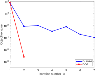
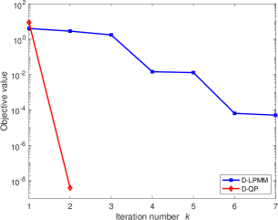
(a)	(b)

Figure 1: The values of $\|\bm{x}^{(k)}\|_{1}^{2}-\alpha^{(k-1)}\|\bm{x}^{(k)}\|^{2}$ against the iteration number $k$. (a) The oversampled DCT sensing matrix with parameters $E=1$, $D=3$, and $s=15$; and (b) The Gaussian sensing matrix with parameters $E=10$, $r=0.2$ and $s=10$.

5.2 Algorithmic Comparison

In this section, we assess the performance of sparse signal recovery algorithms from two perspectives: success rate and user-friendly implementation.

The success rate is calculated as the number of successful trials divided by the total number of trials. A trial is considered successful if the relative error between the ground truth vector $\bm{x}$ and the reconstructed solution $\bm{x}^{*}$, i.e., ${\|\bm{x}^{*}-\bm{x}\|_{2}}/{\|\bm{x}\|_{2}}$ is less than $10^{-3}$.

Figure 2 illustrates the success rate for the oversampled DCT sensing matrix case with $E\in\{1,10,20\}$ and $D\in\{3,5,7\}$. Our proposed algorithms show comparable performance to $L_{1}/L_{2}$-A1 and $L_{1}/L_{2}$-A2. Consistent with the findings in Rahimi-Wang-Dong-Lou:SIAMSC:2019 , we observe that increased coherence results in enhanced sparse recovery performance. Furthermore, as discussed in Wang-Yan-Rahimi-Lou:IEEESP:2020 , algorithms that are scale-invariant generally exhibit improved success rates when operating across higher dynamic ranges. Similarly, Figure 3 displays the success rate for the Gaussian sensing matrix case with $E\in\{1,10,20\}$ and $r\in\{0.2,0.5,0.8\}$. In this case as well, all four algorithms demonstrate comparable success rates. Notably, the D-QP algorithm consistently achieves the best or second-best performance compared to other algorithms.

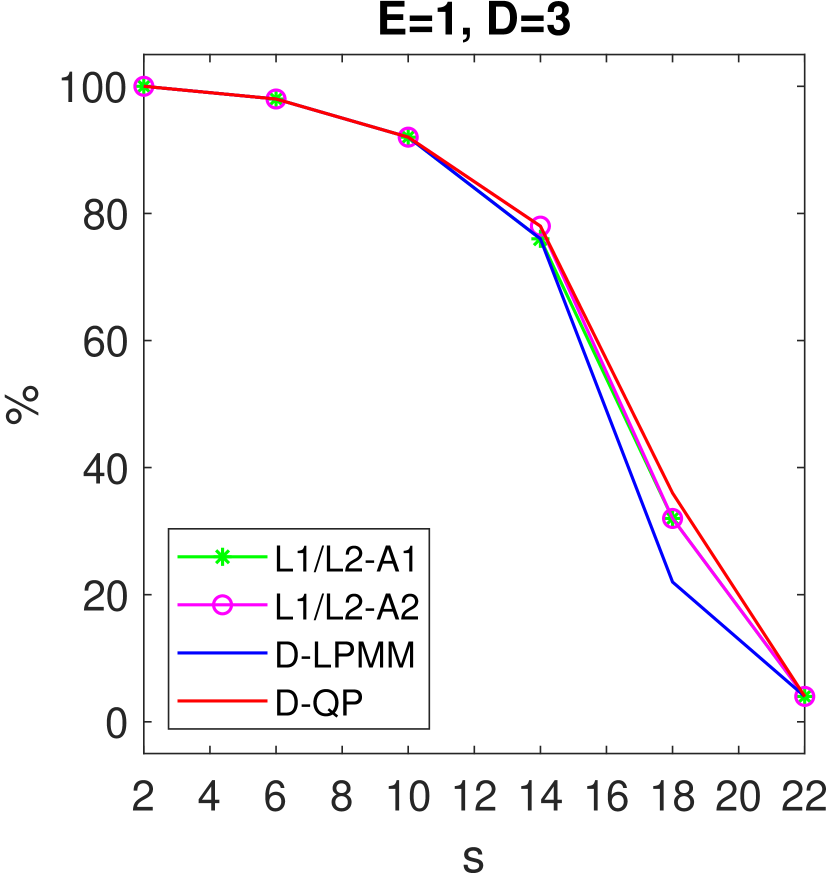
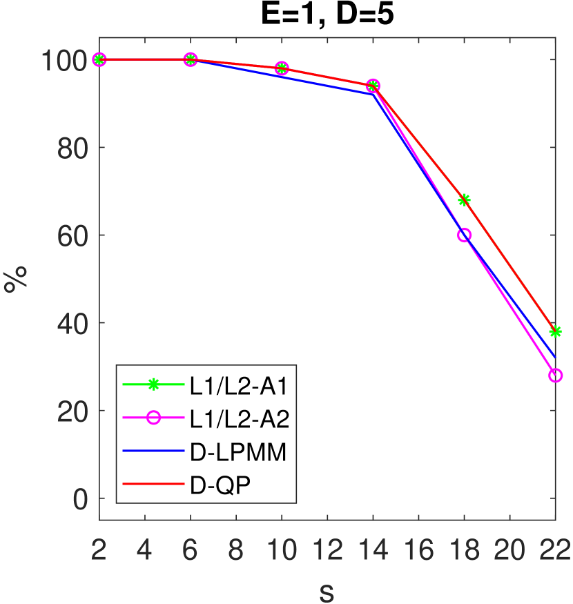
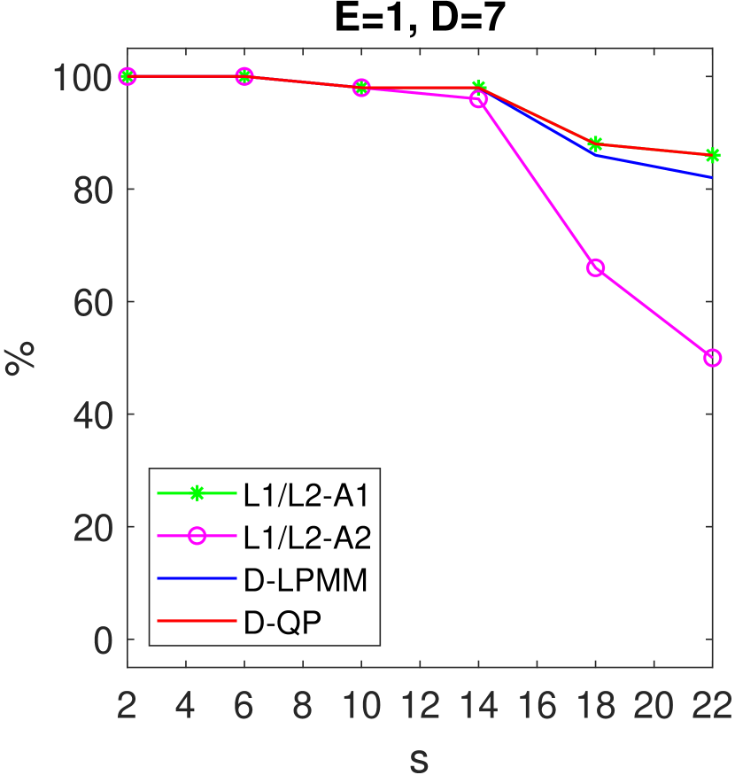
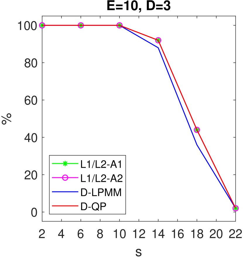
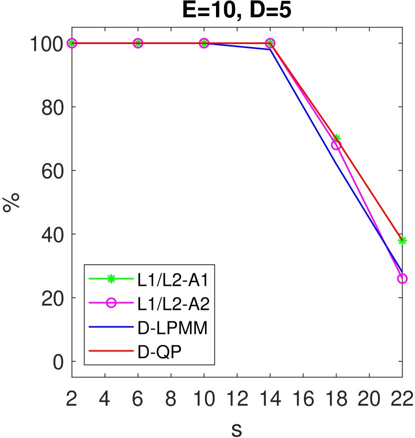
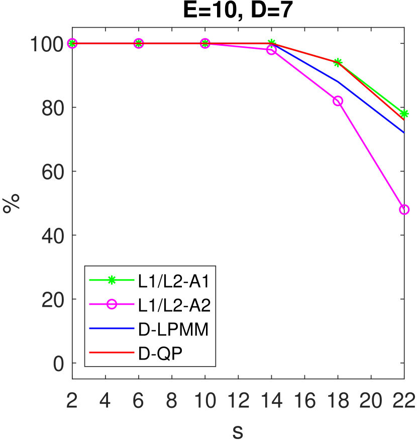
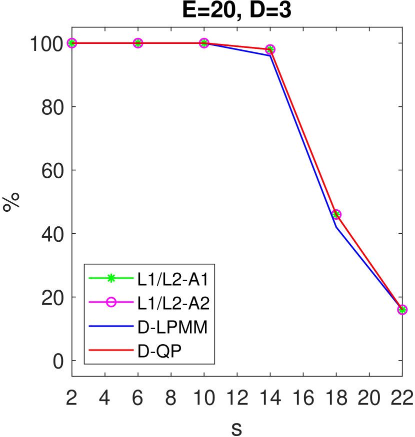
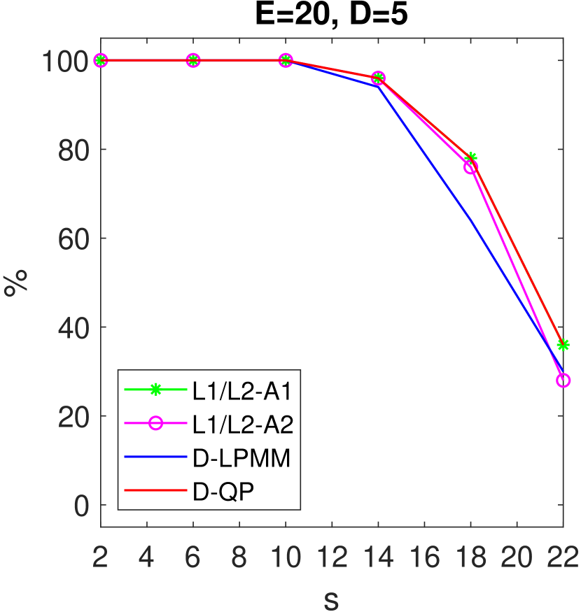
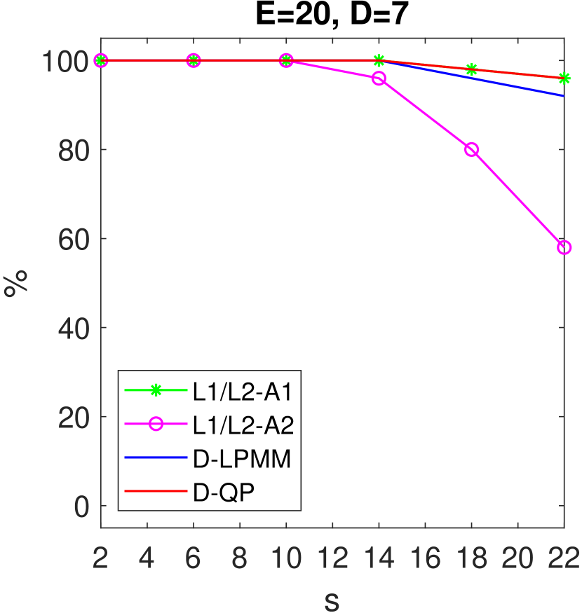
Figure 2: Algorithmic comparison of success rates is conducted for DCT sensing matrices. The presentation of results is structured in a $3\times 3$ grid format, where rows correspond to $E=1,10,20$ from top to bottom, and columns correspond to $D=3,5,7$ from left to right.

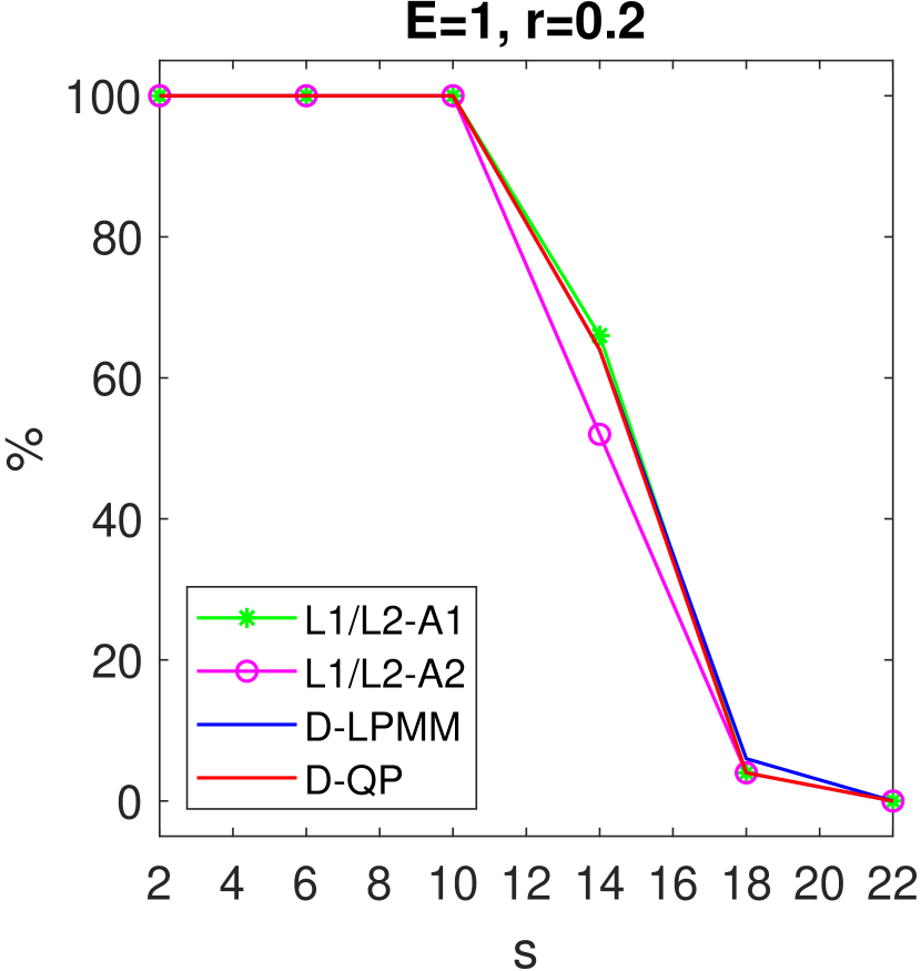
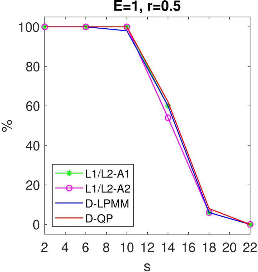
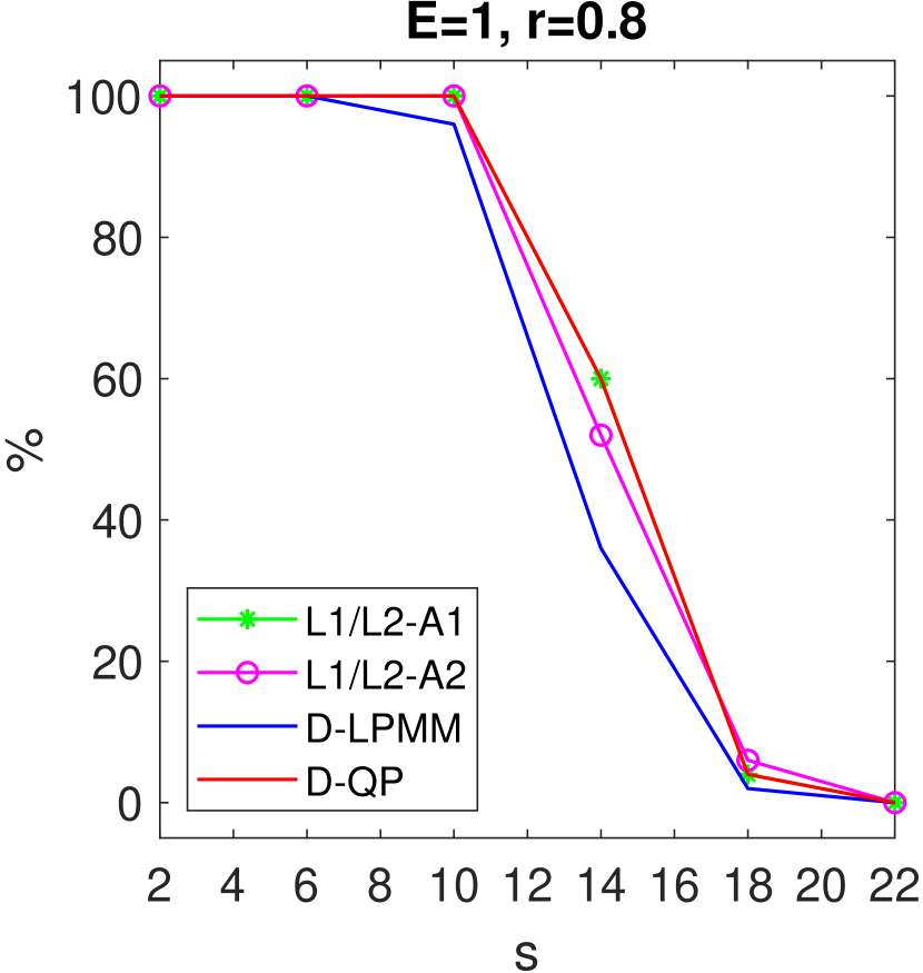
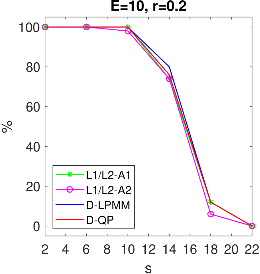
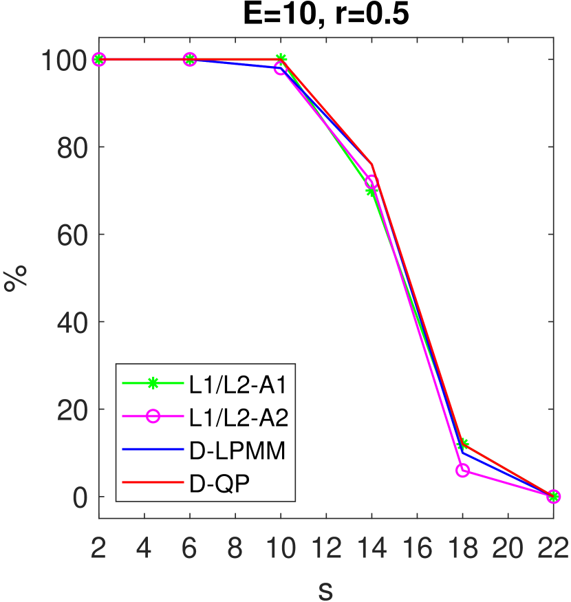
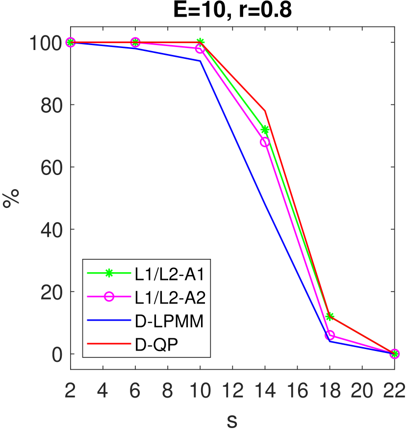
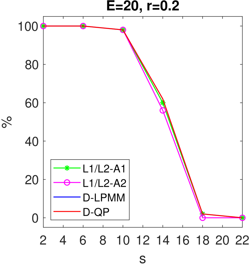
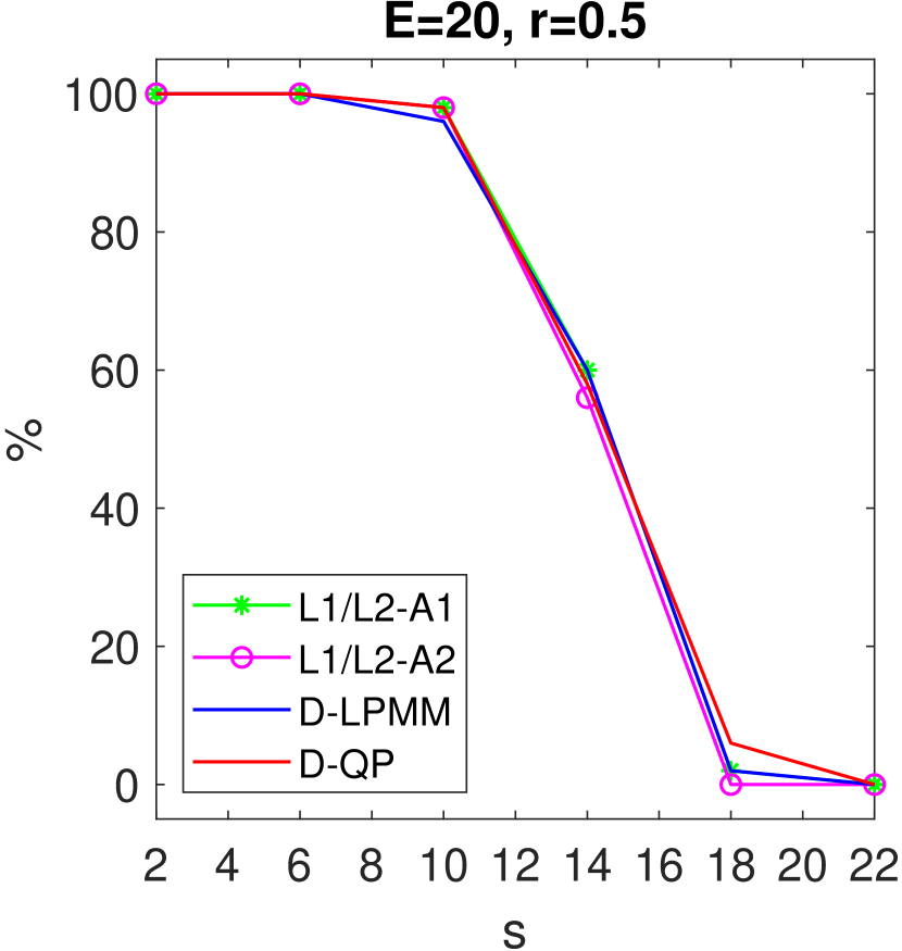
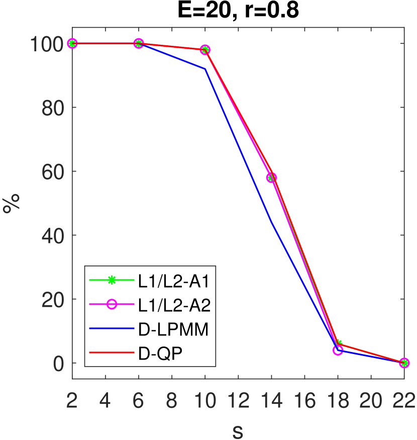
Figure 3: Algorithmic comparison of success rates is conducted for the Gaussian sensing matrices. The presentation of results is structured in a $3\times 3$ grid format, where rows correspond to $E=1,10,20$ from top to bottom, and columns correspond to $r=0.2,0.5,0.8$ from left to right.

For the user-friendly implementation, we emphasize two crucial factors. The first is the number of hyperparameters required by each algorithm. Algorithms that demand fewer hyperparameters simplify the tuning process, enhancing accessibility, particularly for individuals with limited expertise in parameter optimization. This simplicity is vital as it broadens the algorithm’s applicability across diverse scenarios without requiring intricate customization. The second factor is the computational complexity of the algorithms, primarily computational time. Computationally efficient algorithms are preferable in practical scenarios, capable of processing large datasets effectively and suitable for applications with constrained computational resources. These factors are essential in evaluating the algorithms’ practicality and user-friendliness, especially in real-world applications where a balance between accuracy and efficiency is crucial.

The first pivotal factor we discussed for the user-friendly implementation is hyperparameters: D-LPMM was configured with a single parameter, $\lambda$, set to 100 for the oversampled DCT sensing matrices and 2 for Gaussian matrices. In contrast, D-QP, grounded in quadratic programming, operates efficiently without the need for parameter tuning. In implementing the $L_{1}/L_{2}$-A2 approach, we adhered to the recommended configurations for the parameters $\beta$ and $\rho$ in Wang-Yan-Rahimi-Lou:IEEESP:2020 . However, $L_{1}/L_{2}$-A1, despite its linear programming base and apparent lack of parameters, is not without its challenges. As previously discussed in Section 2, it is susceptible to scenarios where the objective function becomes unbounded, resulting in the absence of a viable solution. A further limitation of $L_{1}/L_{2}$-A1 is its lack of a defined convergence analysis, casting doubt on its reliability in consistently reaching a critical point. The specifics of the parameter configurations employed in our study are methodically cataloged in Table I. This delineation underscores the practical superiority of our proposed methods, D-QP’s autonomy from parameterization and D-LPMM’s minimalistic parameter requirement, which markedly simplifies their usage compared to other algorithms that necessitate intricate parameter adjustments for different sensing matrix types.

Table I: Parameters setup for all testing algorithms.

Algorithm	Oversampled DCT	Gaussian
D-QP	Parameter-free	Parameter-free
D-LPMM	$\lambda=100$	$\lambda=2$
$L_{1}/L_{2}$-A1 Wang-Yan-Rahimi-Lou:IEEESP:2020	Parameter-free	Parameter-free
$L_{1}/L_{2}$-A2 Wang-Yan-Rahimi-Lou:IEEESP:2020	$\beta=1$, $\rho=20$	$\beta=10^{-5}$, $\rho=0.3$

The second critical aspect of the user-friendly implementation is computational time. Table II shows the computational time for the oversampled DCT sensing matrix with $(E,D)=(1,3),(10,5)$, and the Gaussian sensing matrix with $(E,r)=(1,0.2),(10,0.5)$. In terms of computational efficiency, both D-LPMM and D-QP show comparable performance, striking an effective balance between speed and ease of use. D-LPMM, with its minimal parameter tuning, and D-QP, operating without any parameters, both demonstrate swift processing capabilities.

Table II: Average computational time (in seconds) for sparse signal recovery.

$s$	$L_{1}/L_{2}$-A1	$L_{1}/L_{2}$-A2	D-LPMM	D-QP	$L_{1}/L_{2}$-A1	$L_{1}/L_{2}$-A2	D-LPMM	D-QP
	Oversampled DCT with $(E,D)=(1,3)$				Oversampled DCT with $(E,D)=(10,5)$
2	0.1777	0.1951	0.1419	0.7693	0.1857	0.1687	0.1497	0.8255
6	0.2004	0.1742	0.1939	0.8696	0.2012	0.1380	0.1903	0.8130
10	0.2245	0.2106	0.2417	0.9159	0.2214	0.1511	0.2340	0.8302
14	0.3297	0.3239	0.4639	1.5123	0.3167	0.1827	0.3385	1.6122
18	0.4993	1.3699	2.1894	3.3791	0.4228	0.2957	0.7576	3.9726
22	0.6525	2.7971	3.7691	6.1085	0.5427	0.6337	1.3844	6.5536
	Gaussian matrix with $(E,r)=(1,0.2)$				Gaussian matrix with $(E,r)=(10,0.5)$
2	0.1929	0.1309	0.2317	0.8362	0.1901	0.1284	0.2537	0.8299
6	0.1977	0.1342	0.4330	0.8376	0.1948	0.1361	1.0063	0.8348
10	0.2359	0.1968	0.6730	1.0305	0.2337	0.1984	1.5466	1.0345
14	0.6772	0.7952	2.0967	3.6477	0.5620	0.7556	3.1580	2.7525
18	1.4552	1.1727	4.3635	8.8977	1.3572	1.1323	4.7501	9.0134
22	1.9751	1.1301	4.7333	13.6945	1.8108	1.1501	4.8884	12.2452

6 Conclusion

In this work, we introduced the $\tau_{2}$-model, a novel approach for sparse signal recovery, which effectively addresses the limitations of the $\ell_{0}$ norm models by utilizing the square of $\ell_{1}/\ell_{2}$ norms. Our study was centered on a thorough exploration of the $\tau_{2}$-model’s properties, delving deep into the intricacies of the corresponding optimization problem, fundamentally rooted in Dinkelbach’s procedure. Through rigorous theoretical analysis and numerical experiments, we have validated the model’s effectiveness in sparse signal recovery. Our numerical experiments highlighted the impact of algorithms developed for the $\tau_{2}$-model on the recovered signals. In our future work, we aim to conduct a more comprehensive study by enhancing D-QP and D-LPMM and incorporating other fractional programming algorithms, such as suggested in Li-Shen-Zhang-Zhou:ACHA-2022 ; Zhang-Li:SIAMOP:2022 .

Conflict of interest

The authors declare that they have no conflict of interest. Any opinions, findings and conclusions or recommendations expressed in this material are those of the authors and do not necessarily reflect the views of AFRL (Air Force Research Laboratory).

References

- (1) Attouch, H., Bolte, J., Svaiter, B.: Convergence of descent methods for semi-algebraic and tame problems: proximal algorithms, forward-backward splitting, and regularized Gauss-Seidel methods. Mathematical Programming, Ser. A 137, 91–129 (2013)
- (2) Beck, A.: First-Order Methods in Optimization. MOS-SIAM Series on Optimization. SIAM (2017)
- (3) Candes, E., Romberg, J., Tao, T.: Robust uncertainty principles: Exact signal reconstruction from highly incomplete frequency information. IEEE Transactions on Information Theory 52(2), 489–509 (2006)
- (4) Chambolle, A., Pock, T.: A first-order primal-dual algorithm for convex problems with applications to imaging. Journal of Mathematical Imaging and Vision 40, 120–145 (2011)
- (5) Chartrand, R.: Exact reconstruction of sparse signals via nonconvex minimization. IEEE Signal Processing Letters 14, 707–710 (2007)
- (6) Chen, F., Shen, L., Suter, B.W.: Computing the proximity operator of the norm with . IET Signal Processing 10, 557–565 (2016)
- (7) Chen, F., Shen, L., Suter, B.W., Xu, Y.: A fast and accurate algorithm for minimization problems in compressive sampling. EURASIP Journal on Advances in Signal Processing 2015 65 (2015)
- (8) Crouzeix, J.P., Ferland, J.A.: Algorithms for generalized fractional programming. Mathematical Programming 52(2), 191–207 (1991)
- (9) Crouzeix, J.P., Ferland, J.A., Schaible, S.: An algorithm for generalized fractional programs. Journal of Optimization Theory and Applications 47(2), 35–49 (1985)
- (10) Donoho, D.: Compressive sensing. IEEE Transanctions on Information Theory 52, 1289?1306 (2006)
- (11) Fannjiang, A., Liao, W.: Coherence pattern–guided compressive sensing with unresolved grids. SIAM Journal on Imaging Sciences 5(1), 179–202 (2012)
- (12) Folland, G.B.: Real analysis: modern techniques and their applications, vol. 40. John Wiley & Sons (1999)
- (13) Hoyer, P.: Non-negative sparse coding. In: Proceedings of the 12th IEEE Workshop on Neural Networks for Signal Processing, pp. 557–565 (2002). DOI 10.1109/NNSP.2002.1030067
- (14) Hurley, N., Rickard, S.: Comparing measures of sparsity. IEEE Transactions on Information Theory 55(10), 4723 – 4741 (2009). DOI 10.1109/TIT.2009.2027527
- (15) Ibaraki, T.: Parametric approaches to fractional programs. Mathematical Programming 26(2), 345–362 (1983)
- (16) Li, Q., Shen, L., Xu, Y., Zhang, N.: Multi-step fixed-point proximity algorithms for solving a class of optimization problems arising from image processing. Advances in Computational Mathematics 41(2), 387–422 (2015)
- (17) Li, Q., Shen, L., Zhang, N., Zhou, J.: A proximal algorithm with backtracked extrapolation for a class of structured fractional programming. Applied and Computational Harmonic Analysis 56, 98–122 (2022)
- (18) Lopes, M.: Estimating unknown sparsity in compressed sensing. In: International Conference on Machine Learning, pp. 217–225. PMLR (2013)
- (19) Lopes, M.E.: Unknown sparsity in compressed sensing: Denoising and inference. IEEE Transactions on Information Theory 62(9), 5145–5166 (2016)
- (20) Prater-Bennette, A., Shen, L., Tripp, E.E.: A constructive approach for computing the proximity operator of the -th power of the -norm. Applied and Computational Harmonic Analysis 67, 101572 (2023)
- (21) Rahimi, Y., Wang, C., Dong, H., Lou, Y.: A scale-invariant approach for sparse signal recovery. SIAM Journal on Scientific Computing 41(6), A3649–A3672 (2019). DOI 10.1137/18M123147X. URL https://doi.org/10.1137/18M123147X
- (22) Shen, L., Suter, B.W., Tripp, E.E.: Structured sparsity promoting functions. Journal of Optimization Theory and Applications 183(3), 386–421 (2019)
- (23) Tang, G., Nehorai, A.: Performance analysis of sparse recovery based on constrained minimal singular values. IEEE Transactions on Signal Processing 59(12), 5734–5745 (2011)
- (24) Wang, C., Yan, M., Rahimi, Y., Lou, Y.: Accelerated schemes for the minimization. IEEE Transactions on Signal Processing 68, 2660–2669 (2020). DOI 10.1109/TSP.2020.2985298
- (25) Yin, P., Esser, E., Xin, J.: Ratio and difference of and norms and sparse representation with coherent dictionaries. Commun. Inf. Syst. 14, 87–109 (2014)
- (26) Yin, P., Lou, Y., He, Q., Xin, J.: Minimization of for compressed sensing. SIAM Journal on Scientific Computing 37(1), A536–A563 (2015)
- (27) Zeng, L., Yu, P., Pong, T.K.: Analysis and algorithms for some compressed sensing models based on l1/l2 minimization. SIAM Journal on Optimization 31(2), 1576–1603 (2021). DOI 10.1137/20M1355380. URL https://doi.org/10.1137/20M1355380
- (28) Zhang, C.H.: Nearly unbiased variable selection under minimax concave penalty. Annals of Statistics 38(2), 894–942 (2010)
- (29) Zhang, N., Li, Q.: First-order algorithms for a class of fractional optimization problems. SIAM Journal on Optimization 32(1), 100–129 (2022). DOI 10.1137/20M1325381
- (30) Zhang, S., Xin, J.: Minimization of transformed penalty: theory, difference of convex function algorithm, and robust application in compressed sensing. Mathematical Programming 169, 307–336 (2018)
- (31) Zhang, X., Burger, M., Osher, S.: A unified primal-dual algorithm framework based on Bregman iteration. Journal of Scientific Computing 46, 20–46 (2011)
- (32) Zhang, Y.: Theory of compressive sensing via -minimization: A non-rip analysis and extensions. Journal of the Operations Research Society of China 1, 79–105 (2013)