Convex Network Flows

Abstract

We introduce a general framework for flow problems over hypergraphs. In our problem formulation, which we call the convex flow problem, we have a concave utility function for the net flow at every node and a concave utility function for each edge flow. The objective is to minimize the sum of these utilities, subject to constraints on the flows allowed at each edge, which we only assume to be a convex set. This framework not only includes many classic problems in network optimization, such as max flow, min-cost flow, and multi-commodity flows, but also generalizes these problems to allow, for example, concave edge gain functions. In addition, our framework includes applications spanning a number of fields: optimal power flow over lossy networks, routing and resource allocation in ad-hoc wireless networks, Arrow-Debreu Nash bargaining, and order routing through financial exchanges, among others. We show that the convex flow problem has a dual with a number of interesting interpretations, and that this dual decomposes over the edges of the hypergraph. Using this decomposition, we propose a fast solution algorithm that parallelizes over the edges and admits a clean problem interface. We provide an open source implementation of this algorithm in the Julia programming language, which we show is significantly faster than the state-of-the-art commercial convex solver Mosek.

1 Introduction

Network flow models describe a wide variety of common scenarios in computer science, operations research, and other fields: from routing trucks to routing bits. An extensive literature has developed theory, algorithms, and applications for the case of linear flows over graphs. (See, e.g., [AMO88], [Wil19], and references therein.) However, the modeling capability of linear network flows is significantly limited. For example, in many applications, the marginal flow out of an edge decreases as the flow into this edge increases; i.e., the output from the edge, as a function of its input, is concave. This property can be observed in physical systems, such as power networks, where increasing the power through a transmission line increases the line’s loss, and in economic systems, such as financial markets, where buying more of an asset increases the price of that asset, resulting in a worse exchange rate. Additionally, there are many applications where the flows through multiple edges connected to a single node are nonlinearly related. For example, in a wireless network, a transmitter has a power constraint across all of its links. Alternatively, in economics, utilities may be superadditive when goods are complements. The fact that classical network flow models cannot incorporate these well-studied applications suggests that there is a natural generalization that can.

In this paper, we introduce the convex flow problem, a generalization of the network flow problem that significantly expands its modeling power. We introduce two key ideas which, taken together, allow our framework to model many additional problems present in the literature. First, instead of a graph, we consider flows over a hypergraph—a graph where an edge may connect more than two vertices. Second, we consider the allowable flows for each edge (which may contain more than two vertices) to be a general convex set. This setup includes, as special cases, the linear relationship studied in most network flow problems and the concave, monotonic increasing edge input-output functions studied in [Shi06, Vég14]. Our framework also encompasses a number of other problems in networked physical and economic systems previously studied in the literature. In many cases, it offers immediate generalizations or more succinct formulations. We outline examples from a number of fields, including power systems, wireless networks, Fisher markets, and financial asset networks.

The convex flow problem we introduce is a convex optimization problem which can, in practice, be efficiently solved. Our framework preserves the overall network structure present in the problem and provides several interesting insights. These insights, in turn, allow us to develop an efficient algorithm for solving the convex flow problem. We show that the dual problem decomposes over the network’s edges, which leads to a highly-parallelizable algorithm that can be decentralized. Importantly, this algorithm has a clean problem interface: we only need access to (1) a Fenchel conjugate-like function of the objective terms and (2) the solution to a simple subproblem for each edge. These subproblem evaluations can be parallelized and have efficiently-computable (and often closed form) solutions in many applications. As a result, our algorithm enjoys better scaling and order-of-magnitude faster solve times than commercial solvers like Mosek.

Outline.

We introduce a general framework for optimizing convex flows over hypergraph structures, where each edge may connect more than two vertices, in section 2. In section 3, we show that this framework encompasses a number of problems previously studied in the literature such as minimum cost flow and routing in wireless networks, and, in some cases, offers immediate generalizations. We find a specific dual problem in section 4, which we show has many useful interpretations and decomposes nicely over the edges of the network. In section 5, we introduce an efficient algorithm that makes use of this decomposition. This algorithm includes an efficient method to handle edges which connect only two nodes, along with a method to recover a solution to the original problem, using the solution to the dual, when the problem is not strictly convex. Finally, we conclude with some numerical examples in section 6. This paper is accompanied by an open source implementation of the solver in the Julia programming language.

1.1 Related work

The classic linear network flow problem has been studied extensively and we refer the reader to [AMO88] and [Wil19] for a thorough treatment. In the classic setting, edges connecting more than two vertices can be modeled by simply augmenting the graph with additional nodes and two-node edges. While nonlinear cost functions have also been extensively explored in the literature (e.g., see [Ber98] and references therein), nonlinear edge flows—when the flow out of an edge is a nonlinear function of the flow into it—has received considerably less attention despite its increased modeling capability.

Nonlinear edge flows.

Extending the network flow problem to include nonlinear edge flows was first considered by Truemper [Tru78]. Still, work in the subsequent decades mainly focused on the linear case—when the flow out of an edge is a linear function of the flow into that edge—possibly with a convex cost function in the objective. (See, for example, [Ber98] and references therein.) More recently, Shigeno [Shi06] and Végh [Vég14] considered the maximum flow problem where the flow leaving and edge is a concave function of the flow entering that edge and proposed theoretically efficient algorithms tailored to this case. This problem is a special case of the convex flow problem we introduce in this work. The nonlinear network flow problem has also appeared in a number of applications, which we refer to in the relevant sections.

Dual decomposition methods for network flows.

The use of dual decomposition methods for network flow problems has a long and rich history, dating back to Kuhn’s ‘Hungarian method’ for the assignment problem [Kuh55]. The optimization community has explored these methods extensively for network optimization problems (e.g., see [Ber98, §6, §9]) and, more generally, for convex optimization problems with coupling constraints (e.g., see [Ber16, §7]). These methods have also been applied to many network problems in practice. For example, they have facilitated the analysis and design of networking protocols, such as those used for TCP congestion control [CLCD07]. These protocols are, in essence, distributed, decentralized algorithms for solving some global optimization problem.

Extended monotropic programming.

Perhaps most related to our framework is the extended monotropic programming problem, introduced by Bertsekas [Ber08], of which our convex flow problem is a special case. Both the convex flow problem and the extended monotropic programming problem generalize Rockafellar’s monotropic programming problem [Roc84]. The strong duality result of [Ber08], therefore, applies to our convex flow problem as well, and we make this connection explicit in appendix A. Although the convex flow problem we introduce is a special case of the extended monotropic programming problem, our work differs from that of Bertsekas along a number of dimensions. First, we construct a different dual optimization problem which has a number of nice properties. Second, this dual leads to a different algorithm than the one developed in [Ber08] and [Ber15, §4], and our dual admits an easier-to-implement interface with simpler ‘subproblems’. Finally, while the application to multi-commodity flows is mentioned in [Ber08], we show that our framework encompasses a number of other problems in networked physical and economic systems previously studied in the literature, and we numerically illustrate the benefit of our approach.

2 The convex flow problem

In this section, we introduce the convex flow problem, which generalizes a number of classic optimization problems in graph theory, including the maximum flow problem, the minimum cost flow problem, the multi-commodity flow problem, and the monotropic programming problem, among others. Our generalization builds on two key ideas: first, instead of a graph, we consider a hypergraph, where each edge can connect more than two nodes, and, second, we represent the set of allowable flows for each edge as a convex set. These two ideas together allow us to model many practical applications which have nonlinear relationships between flows.

Hypergraphs.

We consider a hypergraph with $n$ nodes and $m$ hyperedges. Each hyperedge (which we will refer to simply as an ‘edge’ from here on out) connects some subset of the $n$ nodes. This hypergraph may also be represented as a bipartite graph with $n+m$ vertices, where the first independent set contains $n$ vertices, each corresponding to one of the $n$ nodes in the hypergraph, and the second independent set contains the remaining $m$ vertices, corresponding to the $m$ edges in the hypergraph. An edge in the bipartite graph exists between vertex $i$, in the first independent set, and vertex $j$, in the second independent set, if, and only if, in the corresponding hypergraph, node $i$ is incident to (hyper)edge $j$. Figure 1 illustrates these two representations. From the bipartite graph representation, we can easily see that the labeling of ‘nodes’ and ‘edges’ in the hypergraph is arbitrary, and we will sometimes switch these labels based on convention in the applications. While this section presents the bipartite graph representation as a useful perspective for readers, it is not used in what follows.

Figure 1: A hypergraph with 4 nodes and 3 edges (left) and its corresponding bipartite graph representation (right).

Flows.

On each of the edges in the graph, $i=1,\dots,m$, we denote the flow across edge $i$ by a vector $x_{i}\in\mathbf{R}^{n_{i}}$, where $n_{i}\geq 2$ is the number of nodes incident to edge $i$. Each of these edges $i$ also has an associated closed, convex set $T_{i}\subseteq\mathbf{R}^{n_{i}}$, which we call the allowable flows over edge $i$, such that only flows $x_{i}\in T_{i}$ are feasible. (We often also have that $0\in T_{i}$, i.e., we have the option to not use an edge.) By convention, we will use positive numbers to denote flow out of an edge (equivalently, into a node) and negative numbers to denote flow into an edge (equivalently, out of a node). For example, in a standard graph, every edge connects exactly two vertices, so $n_{i}=2$. If $1$ unit of flow travels from the first node to the second node through an edge, the flow vector across that edge is

$$x_{i}=\begin{bmatrix}-1\\ 1\end{bmatrix}.$$

If this edge is bidirectional (i.e., if flow can travel in either direction), lossless, and has some upper bound $b_{i}>0$ on the flow (sometimes called the ‘capacity’), then its allowable flows are

$$T_{i}=\{z\in\mathbf{R}^{2}\mid z\leq b_{i}\mathbf{1}~{}~{}\text{and}~{}~{}z_{1}+z_{2}=0\}.$$

While this formalism may feel overly cumbersome when dealing with standard graphs, it will be useful for working with hypergraphs.

Local and global indexing.

We denote the number of nodes incident to edge $i$ by $n_{i}$. This set of ‘local’ incident nodes is a subset of the ‘global’ set of $n$ nodes in the hypergraph. To connect the local node indices to the global node indices, we introduce matrices $A_{i}\in\mathbf{R}^{n\times n_{i}}$. In particular, we define $(A_{i})_{jk}=1$ if node $j$ in the global index corresponds to node $k$ in the local index, and $(A_{i})_{jk}=0$, otherwise. For example, consider a hypergraph with 3 nodes. If edge $i$ connects nodes 2 and 3, then

$$A_{i}=\begin{bmatrix}0&0\\ 1&0\\ 0&1\end{bmatrix}=\begin{bmatrix}\vline&\vline\\ e_{2}&e_{3}\\ \vline&\vline\end{bmatrix}.$$

Written another way, if the $k$th node in the edge corresponds to global node index $j$, then the $k$th column of $A_{i}$, is the $j$th unit basis vector, $e_{j}$. Note that the ordering of nodes in the local indices need not be the same as the global ordering.

Net flows.

By summing the flow in each edge, after mapping these flows to the global indices, we obtain the net flow vector

$$y=\sum_{i=1}^{m}A_{i}x_{i}.$$

We can interpret $y$ as the netted flow across the hypergraph. If $y_{j}>0$, then node $j$ ends up with flow coming into it. (These nodes are often called sinks.) Similarly, if $y_{j}<0$, then node $j$ must provide some flow to the network. (These nodes are often called sources.) Note that a node $j$ with $y_{j}=0$ may still have flow passing through it; zero net flow only means that this node is neither a source nor a sink.

Utilities.

Now that we have defined the individual edge flows $x_{i}$ and the net flow vector $y$, we introduce utility functions for each. First, we denote the network utility by $U:\mathbf{R}^{n}\to\mathbf{R}\cup\{-\infty\}$, which maps the net flow vector $y$ to a utility value, $U(y)$. Infinite values denote constraints: any flow with $U(y)=-\infty$ is unacceptable. We also introduce a utility function for each edge, $V_{i}:\mathbf{R}^{n_{i}}\to\mathbf{R}\cup\{-\infty\}$, which maps the flow $x_{i}$ on edge $i$ to a utility, $V_{i}(x_{i})$. We require that both $U$ and the $V_{i}$ are concave, nondecreasing functions. This restriction is not as strong as it may seem; we may also minimize convex nondecreasing cost functions with this framework.

Convex flow problem.

The convex flow problem seeks to maximize the sum of the network utility and the individual edge utilities, subject to the constraints on the allowable flows:

maximize $${\textstyle U(y)+\sum_{i=1}^{m}V_{i}(x_{i})}$$ (1)

subject to $${\textstyle y=\sum_{i=1}^{m}A_{i}x_{i}}$$

$$x_{i}\in T_{i},\quad i=1,\dots,m.$$

Here, the variables are the edge flows $x_{i}\in\mathbf{R}^{n_{i}}$, for $i=1,\dots,m$, and the net flows $y\in\mathbf{R}^{n}$. Each of these edges can be thought of as a subsystem with its own local utility function $V_{i}$. The individual edge flows $x_{i}$ are local variables, specific to the $i$th subsystem. The overall system, on the other hand, has a utility that is a function of the net flows $y$, the global variable. As we will see in what follows, this structure naturally appears in many applications and lends itself nicely to parallelizable algorithms. Note that, because the objective is nondecreasing in all of its variables, a solution $\{x^{\star}_{i}\}$ to problem (1) will almost always have $x_{i}^{\star}$ at the boundary of the feasible flow set $T_{i}$. If an $x_{i}^{\star}$ were in the interior, we could increase its entries without decreasing the objective value until we hit the boundary of the corresponding $T_{i}$, assuming some basic conditions on $T_{i}$ (e.g., $T_{i}$ does not contain a strictly positive ray).

3 Applications

In this section, we give a number of applications of the convex flow problem (1). We first show that many classic optimization problems in graph theory are special cases of this problem. Then, we show that the convex flow problem models problems in a variety of fields including power systems, communications, economics, and finance, among others. We start with simple special cases and gradually build up to those that are firmly outside the traditional network flows literature.

3.1 Maximum flow and friends

In this subsection, we show that many classic network flow problems are special cases of problem (1). We begin with a standard setup that will be used for the rest of this subsection.

Edge flows.

We consider a directed graph with $m$ edges and $n$ nodes, which we assume to be connected. Recall that we denote the flow over edge $i$ by the vector $x_{i}\in\mathbf{R}^{2}$. We assume that edge $i$’s flow has upper bound $b_{i}\geq 0$, so the set of allowable flows is

$$T_{i}=\{z\in\mathbf{R}^{2}\mid 0\leq z_{2}\leq b_{i}~{}~{}\text{and}~{}~{}z_{1}+z_{2}=0\}.$$ (2)

With this framework, it is easy to see how gain factors or other transformations can be easily incorporated into the problem. For example, we can instead require that $\alpha z_{1}+z_{2}=0$ where $\alpha>0$ is some gain or loss factor. Note that if the graph is instead undirected, with each set of two directed edges replaced by one undirected edge, the allowable flows for each pair of directed edges can be combined into the set

$$T_{i}=\{z\in\mathbf{R}^{2}\mid z\leq b_{i}\mathbf{1}~{}~{}\text{and}~{}~{}z_{1}+z_{2}=0\},$$

which is the Minkowski sum of the two allowable flows in the directed case, one for each direction. For what follows, we only consider directed graphs, but the extension to the undirected case is straightforward.

Net flow.

To connect these edge flows to the net flow we use the matrices $A_{i}\in\{0,1\}^{n\times 2}$ for each edge $i=1,\dots,m$ such that, if edge $i$ connects node $j$ to node $k$ (assuming the direction of the edge is from node $j$ to node $k$), then we have

$$A_{i}=\begin{bmatrix}\vline&\vline\\ e_{j}&e_{k}\\ \vline&\vline\end{bmatrix}.$$ (3)

Using these matrices, we write the net flow through the network as the sum of the edge flows:

$$y=\sum_{i=1}^{m}A_{i}x_{i}.$$

Conservation laws.

One important consequence of the definition of the allowable flows $T_{i}$ is that there is a corresponding local conservation law: for any allowable flow $x_{i}\in T_{i}$, we have that

$$\mathbf{1}^{T}x_{i}=(x_{i})_{1}+(x_{i})_{2}=0,$$

by definition of the set $T_{i}$. Since the $A_{i}$ matrices are simply selector matrices, we therefore have that $\mathbf{1}^{T}A_{i}x_{i}=0$ whenever $x_{i}\in T_{i}$, which means that we can turn the local conservation law above into a global conservation law:

$$\mathbf{1}^{T}y=\sum_{i=1}^{m}\mathbf{1}^{T}A_{i}x_{i}=0,$$ (4)

where $y$ is the corresponding net flow, for any set of allowable flows $x_{i}\in T_{i}$, for $i=1,\dots,m$. We will use this fact to show that feasible flows are, indeed, flows through the network in the ‘usual’ sense.

3.1.1 Maximum flow

Given a directed graph, the maximum flow problem seeks to find the maximum amount of flow that can be sent from a designated source node to a designated sink node. The problem can model many different situations, including transportation network routing, matching, and resource allocation, among others. It dates back to the work of Harris and Ross [HR55] to model Soviet railway networks in a report written for the US Air Force and declassified in 1999, at the request of Schrijver [Sch02]. While well-known to be a linear program at the time [FF56] (and therefore solvable with the simplex method), specialized methods were quickly developed [FF57]. The maximum flow problem has been extensively studied by the operations research and computer science communities since then.

Flow conservation.

Relabeling the graph such that the source node is node $1$ and the sink node is node $n$, we write the net flow conservation constraints as the set

$$S=\{y\in\mathbf{R}^{n}\mid y_{1}+y_{n}\geq 0,\quad y_{j}\geq 0\quad\text{for all}~{}~{}j\neq 1,n\}.$$ (5)

Note that this set $S$ is convex as it is the intersection of halfspaces (each of which is convex), and its corresponding indicator function, written

$$I_{S}(y)=\begin{cases}0&y\in S\\ +\infty&\text{otherwise},\end{cases}$$

is therefore also convex. This indicator function is nonincreasing in that, if $y^{\prime}\geq y$ then $I_{S}(y^{\prime})\leq I_{S}(y)$ by definition of the set $S$. Thus, its negation, $-I_{S}$, is nondecreasing and concave.

Problem formulation.

The network utility function in the maximum flow problem is to maximize the flow into the terminal node while respecting the flow conversation constraints:

$$U(y)=y_{n}-I_{S}(y).$$

From the previous discussion, this utility function is concave and nondecreasing. We set the edge utility functions to be zero, $V_{i}=0$ for all $i=1,\dots,m$, to recover the maximum flow problem (see, for example, [Ber98, Example 1.3]) in our framework:

maximize $$y_{n}-I_{S}(y)$$ (6)

subject to $${\textstyle y=\sum_{i=1}^{m}A_{i}x_{i}}$$

$$x_{i}\in T_{i},\quad i=1,\dots,m,$$

where the sets $\{T_{i}\}$ are the feasible flow sets (2) and may be either directed or undirected.

Problem properties.

Any feasible point (i.e., one that satisfies the constraints and has finite objective value) is a flow in that the net flow through node $j$ is zero ($y_{j}=0$) for any node that is not the source, $j=1$, or the sink, $j=n$. To see this, note that, for any $j\neq 1,n$, if $y\in S$, then

$$\mathbf{1}^{T}y\geq y_{1}+y_{n}+y_{j}\geq y_{j}\geq 0.$$

The first and third inequalities follow from the fact that $y\in S$ means that $y_{j}\geq 0$ for all $j\neq 1,n$; the second follows from the fact that $y_{1}+y_{n}\geq 0$ from the definition of $S$ as well. From the conservation law (4), we know that $\mathbf{1}^{T}y=0$, so $y_{j}=0$ for every node $j$ that is not the source nor the sink. Therefore, $y$ is a flow in the ‘usual’ sense. A similar proof shows that $-y_{1}=y_{n}$; i.e., the amount provided by the source is the amount dissipated by the sink. Since we are maximizing the total amount dissipated $y_{n}$, subject to the provided capacity and flow constraints, the problem above corresponds exactly to the standard maximum flow problem.

3.1.2 Minimum cost flow

The minimum cost flow problem seeks to find the cheapest way to route a given amount of flow between specified source and sink nodes. We consider the same setup as above, but with two modifications: first, we fix the value of the flow from node $1$ to node $n$ to be at least some value $v\geq 0$; and second, we introduce a convex, nondecreasing cost function for each edge $i$, denoted $c_{i}:\mathbf{R}_{+}\to\mathbf{R}_{+}$, which maps the flow on this edge to a cost. We modify the flow conservation constraints to be (cf., (5))

$$\tilde{S}=\{y\mid y_{n}\geq v,\quad y_{1}+y_{n}\geq 0,\quad y_{j}\geq 0\quad\text{for all}~{}~{}j\neq 1,n\}.$$

Much like the previous, the negative indicator of this set, $-I_{\tilde{S}}$, is a concave, nondecreasing function. We take the edge flow utility function $V_{i}$ to be

$$V_{i}(x_{i})=-c_{i}(-(x_{i})_{1}),$$

which is a concave nondecreasing function of $x_{i}$. (Recall that $(x_{i})_{1}\leq 0$. We provide an example in figure 2.) Modifying the network utility function to be the indicator over this new set $\tilde{S}$,

$$U(y)=-I_{\tilde{S}}(y),$$

we recover the minimum cost flow problem in our framework:

maximize $${\textstyle{-I_{\tilde{S}}(y)}+\sum_{i=1}^{m}-c_{i}(-(x_{i})_{1})}$$

subject to $${\textstyle y=\sum_{i=1}^{m}A_{i}x_{i}}$$

$$x_{i}\in T_{i},\quad i=1,\dots,m.$$

Here, as before, the sets $\{T_{i}\}$ are the directed feasible flow sets defined in (2).

Figure 2: An example convex nondecreasing cost function $c(w)=w^{2}$ for $w\geq 0$ (left) and its corresponding concave, nondecreasing edge utility function $V$ (right).

3.1.3 Concave edge gains

We can generalize the maximum flow problem and the minimum cost flow problem to include concave, nondecreasing edge input-output functions, as in [Shi06, Vég14], by modifying the sets of feasible flows. We denote the edge input-output functions by $\gamma_{i}:\mathbf{R}_{+}\to\mathbf{R}_{+}$. (For convenience, negative arguments to $\gamma_{i}$ are equal to negative infinity.) If $w$ units of flow enter edge $i$, then $\gamma_{i}(w)$ units of flow leave edge $i$. In this case, we can write the set of allowable flows for each edge to be

$$T_{i}=\{z\in\mathbf{R}^{2}\mid z_{2}\leq\gamma_{i}(-z_{1})\}.$$

We provide an example in figure 3. The inequality has the following interpretation: the magnitude of the flow out of edge $i$, given by $z_{2}\geq 0$, can be any value not exceeding $\gamma_{i}(-z_{1})$; however, we can ‘destroy’ flow. From the problem properties presented in section 2, there exists a solution such that this inequality is tight, since the utility function $U$ is nondecreasing. In other words, we can find a set of feasible flows $\{x_{i}\}$ such that

$$(x_{i})_{2}=\gamma_{i}(-(x_{i})_{1}),$$

for all edges $i=1,\dots,m$.

Figure 3: An example concave edge gain function $\gamma(w)=\sqrt{w}$ (left) and the corresponding allowable flows (right).

3.1.4 Multi-commodity flows

Thus far, all the flows have been of the same type. Here, we show that the multi-commodity flow problem, which seeks to route $K$ different commodities through a network in an optimal way, is also a special case of the convex flow problem. We denote the flow of these commodities over an edge $i$ by $x_{i}\in\mathbf{R}^{2K}$, where the first $2$ elements denote the flow of the first commodity through edge $i$, the next $2$ elements denote the flow of the second, and so on. The set $T_{i}$ then allows us to specify joint constraints on these flows. For example, we can model a total flow capacity by the set

$$T_{i}=\left\{x\in\mathbf{R}^{K}~{}\middle|~{}\sum_{k=1}^{K}w_{k}x_{2k}\leq b_{i},~{}0\leq x_{2k},~{}\text{and}~{}x_{2k}=-x_{2k-1}~{}\text{for}~{}k=1,2,\dots,K\right\},$$

where $b_{i}$ denotes the capacity of edge $i$ and $w_{k}$ denotes the capacity required per unit of commodity $k$. In other words, each commodity $k$ has a per-unit ‘weight’ of $w_{k}$, and the maximum weighted capacity through edge $i$ is $b_{i}$. If $K=1$, then this set of allowable flows reduces to the original definition (2). Additionally, note that $T_{i}$ is still a polyhedral set, but more complicated convex constraints may be added as well.

We denote the net flows at each node by a vector $y\in\mathbf{R}^{nK}$, where the first $K$ elements denote the net flows of the first commodity, the next $K$ elements denote the net flows of the second, and so on, while the $A_{i}$ matrices map the local flows of each good to the corresponding indices in $y$. For example, if edge $i$ connects node $j$ to node $k$, the edge would have the associated matrix $A_{i}\in\mathbf{R}^{nK\times 2K}$ given by

$$A_{i}=\begin{bmatrix}\vline&\vline&\vline&\vline&&\vline&\vline\\ e_{j}&e_{k}&e_{j+n}&e_{k+n}&\cdots&e_{j+(K-1)n}&e_{k+(K-1)n}\\ \vline&\vline&\vline&\vline&&\vline&\vline\end{bmatrix}.$$

The problem is now analogous to those in the previous sections, only with $y$ and $x_{i}$ having larger dimension and $T_{i}$ modified as described above.

3.2 Optimal power flow

The optimal power flow problem [WWS13] seeks a cost-minimizing plan to generate power satisfying demand in each region. We consider a network of $m$ transmission lines (edges) between $n$ regions (nodes). We assume that the region-transmission line graph is directed for simplicity.

Line flows.

When power is transmitted along a line, the line heats up and, as a result, dissipates power. As greater amounts of power are transmitted along this line, the line further heats up, which, in turn, causes it to dissipate even more power. We model this dissipation as a convex function of the power transmitted, which captures the fact that the dissipation increases as the power transmitted increases. We use the logarithmic power loss function from [Stu19, §2.1.3]. With this loss function, the ‘transport model’ optimal power flow solution matches that of the more-complicated ‘DC model’, assuming a uniform line material. (See [Stu19, §2] for details and discussion.) The logarithmic loss function is given by

$$\ell_{i}(w)=\alpha_{i}\left(\log(1+\exp(\beta_{i}w))-\log 2\right)-2w,$$

where $\alpha_{i}$ and $\beta_{i}$ are known constants and $\alpha_{i}\beta_{i}=4$ for each line $i$. This function can be easily verified to be convex, increasing, and have $\ell_{i}(0)=0$. The power output of a line with input $w$ can then be written as $w-\ell(w)$. We also introduce capacity constraints for each line $i$, given by $b_{i}$. Taken together, for a given line $i$, the power flow $x_{i}$ must lie within the set

$$T_{i}=\left\{z\in\mathbf{R}^{2}\mid-b_{i}\leq z_{1}\leq 0~{}\text{and}~{}z_{2}\leq-z_{1}-\ell_{i}(-z_{1})\right\},\qquad i=1,\dots,m.$$ (7)

This set is convex, as it is the intersection of two halfspaces and the epigraph of a convex function. Note that we relaxed the line flow constraint to an inequality. This inequality has the following physical interpretation: we may dissipate additional power along the line (for example, by adding a resistive load), but in general we expect this inequality to hold with equality, as discussed in §2. Figure 4 shows a loss function and the corresponding edge’s allowable flows.

Figure 4: The power loss function (left), the corresponding power output (middle), and the corresponding set of allowable flows (right).

Net flows.

Each region $i=1,\dots,n$ demands $d_{i}$ units of power. In addition, region $i$ can generate power $p_{i}$ at cost $c_{i}:\mathbf{R}\to\mathbf{R}_{+}\cup\{\infty\}$, where infinite values denote constraints (e.g., a region may have a maximum power generation capacity). We assume that $c_{i}$ is convex and nondecreasing, with $c_{i}(p_{i})=0$ for $p_{i}\leq 0$ (i.e., we can dissipate power at zero cost). Similarly to the max flow problem in §3.1, we take the indexing matrices $A_{i}$ as defined in (3). To meet demand, we must have that

$$d=p+y,\qquad\text{where}\qquad y=\sum_{i=1}^{m}A_{i}x_{i}.$$

In other words, the power produced, plus the net flow of power, must satisfy the demand in each region. We write the network utility function as

$$U(y)=\sum_{i=1}^{n}-c_{i}(d_{i}-y_{i}).$$ (8)

Since each $c_{i}$ is convex and nondecreasing, the utility function $U$ is concave and nondecreasing in $y$. This problem can then be cast as a special case of the convex flow problem (1):

maximize $${\textstyle\sum_{i=1}^{n}-c_{i}(d_{i}-y_{i})}$$

subject to $${\textstyle y=\sum_{i=1}^{m}A_{i}x_{i}}$$

$$x_{i}\in T_{i},\quad i=1,\dots,m,$$

with the same variables $\{x_{i}\}$ and $y$, zero edge utilities ($V_{i}=0$), and the feasible flow sets $T_{i}$ given in (7).

Extensions and related problems.

This model can be extended in a variety of ways. For example, a region may have some joint capacity over all the power it outputs. When there are constraints such as these resulting from the interactions between edge flows, a hypergraph model is more appropriate. On the other hand, simple two-edge concave flows model behavior in number of other types of networks: in queuing networks, throughput is a concave function of the input due to convex delays [BG92, §5.4]; similarly, in routing games [Rou07, §18], a convex cost function often implies a concave throughput; in perishable product supply chains, such as those for produce, increased volume leads to increased spoilage [NB22, §2.3]; and in reservoir networks [Ber98, §8.1], seepage may increase as volume increases. Our framework not only can model these problems, but also allows us to easily extend them to more complicated settings.

3.3 Routing and recourse allocation in wireless networks

In many applications, standard graph edges do not accurately capture interactions between multiple flows coming from a single node—there may be joint, possibly nonlinear, constraints on all the flows involving this node. To represent these constraints in our problem, we make use of the fact that an edge may connect more than two nodes in (1). In this section, we illustrate this structure through the problem of jointly optimizing the data flows and the power allocations for a wireless network, heavily inspired by the formulation of this problem in [XJB04].

Figure 5: Wireless ad-hoc network. The (outgoing) hyperedge associated with user $u$ is shown in blue, and the corresponding set of outgoing neighbors $O_{u}$ contains user $v$ and the two base stations, $b_{1}$ and $b_{2}$.

Data flows.

We represent the topology of a data network by a directed graph with $n$ nodes and $m=n$ edges: one for each node. We want to route traffic from a particular source to a particular destination in the network. (This model can be easily extended to handle multiple source-destination pairs, potentially with different latency or bandwidth constraints, using the multi-commodity flow ideas discussed in §3.1.4.) We model the network with a hypergraph, where edge $i=1,\dots,n$ is associated with node $i$ and connects $i$ to all its outgoing neighbors, which we denote by the set $O_{i}$, as shown in figure 5. (In other words, if $j\in O_{i}$, then node $j$ is a neighbor of node $i$.) On each edge, we have a rate at which we transmit data, denoted by a vector $x_{i}\in\mathbf{R}^{\lvert{O_{i}}\rvert+1}$, where the $k$th element of $x_{i}$ denotes the rate from node $i$ to its $k$th outgoing neighbor and the last component is the total outgoing rate from node $i$. The net flow vector $y\in\mathbf{R}^{n}$ can be written as

$$y=\sum_{i=1}^{n}A_{i}x_{i},$$

for indexing matrices $A_{i}$ in $\mathbf{R}^{n\times(|O_{i}|+1)}$, given by

$$A_{i}=\begin{bmatrix}\vline&&\vline&\vline\\ e_{O_{i1}}&\dots&e_{O_{i|O_{i}|}}&e_{i}\\ \vline&&\vline&\vline\end{bmatrix},$$

where $O_{ik}$ denotes the $k$th neighbor of $O_{i}$ in any order fixed ahead of time.

Communications constraints.

Hyperedges allow us to more easily model the communication constraints in the examples of [XJB04]. We associate some communication variables with each edge $i$. These variables might be, for example, power allocations, bandwidth allocations, or time slot allocations. We assume that the joint constraints on the transmission rate and the communication variables are some convex set. For example, take the communication variables to be $(p_{i},w_{i})$, where $p\in\mathbf{R}^{\lvert{O_{i}}\rvert}$ is a vector of power allocations and $w\in\mathbf{R}^{\lvert{O_{i}}\rvert}$ is a vector of bandwidth allocations to each of node $i$’s outgoing neighbors. We may have maximum power and bandwidth constraints, given by $p^{\mathrm{max}}_{i}$ and $w^{\mathrm{max}}_{i}$, so the set of feasible powers and bandwidths is

$$P_{i}=\{(p,w)\in\mathbf{R}^{\lvert{O_{i}}\rvert}\times\mathbf{R}^{\lvert{O_{i}}\rvert}\mid~{}p\geq 0,~{}w\geq 0,~{}\mathbf{1}^{T}p\leq p^{\mathrm{max}},~{}\mathbf{1}^{T}w\leq w^{\mathrm{max}}\}.$$

These communication variables determine the rate at which node $i$ can transmit data to its neighbors. For example, in the Gaussian broadcast channel with frequency division multiple access, this rate is governed by the Shannon capacity of a Gaussian channel [Sha48]. The set of allowable flows can be written as

$$T_{i}=\left\{(z,t)\in\mathbf{R}^{\lvert{O_{i}}\rvert}\times\mathbf{R}~{}\middle|~{}\mathbf{1}^{T}z=-t,~{}~{}z\leq w\circ\log_{2}\left(\mathbf{1}+\frac{p}{\sigma w}\right),~{}~{}(p,w)\in P_{i}\right\},$$

where $\sigma\in\mathbf{R}_{+}^{n}$ is a parameter that denotes the average power of the noise in each channel, the logarithm and division, along with the inequality, are applied elementwise, and $\circ$ denotes the elementwise (Hadamard) product. The set $T_{i}$ is a convex set, as the logarithm is a concave function and $w_{k}\log(1+p_{k}/\sigma w_{k})$, viewed as a function over the $k$th element of each of the communication variables $(p,w)$, is the perspective transformation of $\log(1+p_{k}/\sigma)$, viewed as a function over $p_{k}$, which preserves concavity [BV04, §3.2.6]. The remaining sets are all affine or polyhedral, and intersections of convex sets are convex, which gives the final result.

Importantly, the communication variables (here, the power allocations $p$ and bandwidth allocations $w$) can be private to a node $i$; the optimizer only cares about the resulting public data flow rates $x_{i}\in T_{i}$. This structure not only simplifies the problem formulation but also hints at efficient, decentralized algorithms to solve this problem. We note that the hypergraph model allows us to also consider the general multicast case as well.

The optimization problem.

Without loss of generality, denote the source node by $1$ and the sink node by $n$. We may simply want to maximize the rate of data from the source to the sink, in which case we can take the network utility function to be

$$U(y)=y_{n}-I_{S}(y),$$

where the flow conversation constraints $S$ are the same as those of the classic maximum flow problem, defined in (5). We may also use the functions $V_{i}$ to include utilities or costs associated with the transmission of data by node $i$. We can include communication variables in the objective as well by simply redefining the allowable flows $T_{i}$ to include the relevant communication variables and modifying the $A_{i}$’s accordingly to ignore these entries of $x_{i}$. This modification is useful when we have costs associated with these variables—for example, costs on power consumption. Equipped with the set of allowable flows and these utility functions, we can write this problem as a convex flow problem (1).

Related problems.

Many different choices of the objective function and constraint sets for communication network allocation problems appear in the literature [XJB04, Ber98]. This setup also encompasses a number of other ‘resource allocation’ problems where the network structure isn’t immediately obvious, one of which we discuss in the next section.

3.4 Market equilibrium and Nash bargaining

Our framework includes and generalizes the concave network flow model used by Végh [Vég14] to study market equilibrium problems such as Arrow-Debreu Nash bargaining [Vaz12]. Consider a market with a set of $n_{b}$ buyers and $n_{g}$ goods. There is one divisible unit of each good to be sold. Buyer $i$ has a budget $b_{i}\geq 0$ and receives utility $u_{i}:\mathbf{R}^{n_{g}}_{+}\to\mathbf{R}_{+}$ from some allocation $x_{i}\in[0,1]^{n_{g}}$ of goods. We assume that $u_{i}$ is concave and nondecreasing, with $u_{i}(0)=0$ for each $i=1,\dots,n_{b}$. An equilibrium solution to this market is an allocation of goods $x_{i}\in\mathbf{R}^{n_{g}}$ for each buyer $i=1,\dots,n_{b}$, and a price $p_{j}\in\mathbf{R}_{+}$ for each good $j=1,\dots,n_{g}$, such that: (1) all goods are sold; (2) all money of all buyers is spent; and (3) each buyer buys a ‘best’ (i.e., utility-maximizing) bundle of goods, given these prices.

An equilibrium allocation for this market is given by a solution to the following convex program:

maximize $$\sum_{i=1}^{n_{b}}b_{i}\log(u_{i}(x_{i}))$$ (9)

subject to $$\sum_{i=1}^{n_{b}}(x_{i})_{j}=1,\quad j=1,\dots,n_{g}$$

$$x_{i}\geq 0,\quad i=1,\dots,n_{b}.$$

Eisenberg and Gale [EG59] proved that the optimality conditions of this convex optimization problem give the equilibrium conditions in the special case that $u_{i}(x)$ is linear (and therefore separable across goods), i.e.,

$$u_{i}(x_{i})=v_{i}^{T}x_{i}$$

for constant weights $v_{i}\in\mathbf{R}_{+}^{n_{g}}$. (We show the same result for the general case (9) in appendix B.) The linear case is called the ‘linear Fisher market model’ [Vaz07] and can be easily recognized as a special case of the standard maximum flow problem (6) with nonnegative edge gain factors [Vég14, §3].

Végh showed that all known extensions of the linear Fisher market model are a special case of the generalized market problem (9), where the utility functions $u_{i}$ are separable across the goods, i.e.,

$$u_{i}(x_{i})=\sum_{j=1}^{n_{g}}u_{ij}((x_{i})_{j})$$

for $u_{ij}:\mathbf{R}\to\mathbf{R}$ concave and increasing. Végh casts this problem as a maximum network flow problems with concave edge input-output functions. We make a further extension here by allowing the utilities to be concave nondecreasing functions of the entire basket of goods rather than sums of functions of the individual allocations. This generalization allows us to model complementary goods and is an immediate consequence of our framework.

Figure 6: Network representation of the linear Fisher market model, where we aim to maximize the utility of the net flows $y$. Colored edges represent the $n_{b}+1$ hyperedges connecting each buyer to all the goods, so each of these edges is incident to $n_{g}+1$ vertices. Flows on the right indicate that there is at most one unit of each good to be divided among the buyers.

The convex flow problem.

This problem can be turned into a convex flow problem in a number of ways. Here, we follow Végh [Vég14] and use a similar construction. First, we represent both the $n_{b}$ buyers and $n_{g}$ goods as nodes on the graph: the buyers are labeled as nodes $1,\dots,n_{b}$, and the goods are labeled as nodes $n_{b}+1,\dots,n_{b}+n_{g}$. For each buyer $i=1,\dots,n_{b}$, we introduce a hyperedge connecting buyer $i$ to all goods $j=n_{b}+1,\dots,n_{b}+n_{g}$. We denote the flow along this edge by $x_{i}\in\mathbf{R}^{n_{g}+1}$, where $(x_{i})_{j}$ is the amount of the $j$th good bought by the $i$th buyer, and $(x_{i})_{n_{g}+1}$ denotes the amount of utility that buyer $i$ receives from this basket of goods denoted by the first $n_{g}$ entries of $x_{i}$. The flows on this edge are given by the convex set

$$T_{i}=\left\{(z,t)\in\mathbf{R}^{n_{g}}\times\mathbf{R}\mid-\mathbf{1}\leq z\leq 0,~{}~{}t\leq u_{i}(-z)\right\}.$$ (10)

This set converts the ‘goods’ flow into a utility flow at each buyer node $i$. This setup is depicted in figure 6. Since the indices $1,\dots,n_{b}$ of the net flow vector $y\in\mathbf{R}^{n_{g}+n_{b}}$ correspond to the buyers and the elements $n_{b}+1,\dots,n_{g}+n_{b}$ to correspond to the goods, the utility function above can be written

$$U(y)=\sum_{i=1}^{n_{b}}b_{i}\log(y_{i})-I(y_{n_{b}+1:n_{b}+n_{g}}\geq-\mathbf{1}),$$ (11)

which includes the implicit constraint that at most one unit of each good can be sold in the indicator function $I$, above, and where $y_{n_{b}+1:n_{b}+n_{g}}$ is a vector containing only the $(n_{b}+1)$st to the $(n_{b}+n_{g})$th entries of $y$. Since $U$ is nondecreasing and concave in $y$, $V_{i}=0$, and the $T_{i}$ are convex, we know that (9) is a special case of the convex flow problem (1).

Related problems.

A number of other resource allocation can be cast as generalized network flow problems. For example, Agrawal et al. [ABNKZ22] consider a price adjustment algorithm for allocating compute resources to a set of jobs, and Schutz et al. [STA09] do the same for supply chain problems. In many problems, network structure implicitly appears if we are forced to make decisions over time or over decision variables which directly interact only with a small subset of other variables.

3.5 Routing orders through financial exchanges

Financial asset networks are also well-modeled by convex network flows. If each asset is a node and each market between assets is an edge between the corresponding nodes, we expect the edge input-output functions to be concave, as the price of an asset is nondecreasing in the quantity purchased. In many markets, this input-output function is probabilistic; the state of the market when the order ‘hits’ is unknown due to factors such as information latency, stale orders, and front-running. However, in certain batched exchanges, including decentralized exchanges running on public blockchains, this state can be known in advance. We explore the order routing problem in this decentralized exchange setting.

Decentralized exchanges and automated market makers.

Automated market makers have reached mass adoption after being implemented as decentralized exchanges on public blockchains. These exchanges (including Curve Finance [Ego19], Uniswap [AZR20], and Balancer [MM19], among others) have facilitated trillions of dollars in cumulative trading volume since 2019 and maintain a collective daily trading volume of several billion dollars. These exchanges are almost all implemented as constant function market markers (CFMMs) [AC20, ACDEK23]. In CFMMs, liquidity providers contribute reserves of assets. Users can then trade against these reserves by tendering a basket of assets in exchange for another basket. CFMMs use a simple rule for accepting trades: a trade is only valid if the value of a given function at the post-trade reserves is equal to the value at the pre-trade reserves. This function is called the trading function and gives CFMMs their name.

Constant function market makers.

A CFMM which allows $r$ assets to be traded is defined by two properties: its reserves $R\in\mathbf{R}^{r}$, which denotes the amount of each asset available to the CFMM, and its trading function $\varphi:\mathbf{R}^{r}\to\mathbf{R}$, which specifies its behavior and includes a fee parameter $0<\gamma\leq 1$, where $\gamma=1$ denotes no fee. We assume that $\varphi$ is concave and nondecreasing. Any user is allowed to submit a trade to a CFMM, which we write as a vector $z\in\mathbf{R}^{r}$, where positive entries denote values to be received from the CFMM and negative entries denote values to be tendered to the CFMM. (For example, if $r=2$, then a trade $z=(-1,10)$ would denote that the user wishes to tender $1$ unit of asset $1$ and receive $10$ units of asset $2$.) The submitted trade is then accepted if the following condition holds:

$$\varphi(R-\gamma z_{-}-z_{+})\geq\varphi(R),$$

and $R-\gamma z_{-}-z_{+}\geq 0$. Here, we denote $z_{+}$ to be the ‘elementwise positive part’ of $x$, i.e., $(z_{+})_{j}=\max\{z_{j},0\}$ and $z_{-}$ to be the ‘elementwise negative part’ of $x$, i.e., $(z_{-})_{j}=\min\{z_{j},0\}$ for every asset $j=1,\dots,r$. Note that, since $\varphi$ is concave, the set of acceptable trades is a convex set:

$$T=\{z\in\mathbf{R}^{r}\mid\varphi(R-\gamma z_{-}-z_{+})\geq\varphi(R)\},$$

as we can equivalently write it as

$$T=\{z\in\mathbf{R}^{r}\mid\varphi(R+\gamma u-v)\geq\varphi(R),~{}u,v\geq 0,~{}z=v-u\},$$

which is easily seen to be a convex set since $\varphi$ is a concave function.

Net trade.

Consider a collection of $m$ CFMMs, each of which trades a subset of $n$ possible assets. Denoting the trade with the $i$th CFMM by $x_{i}$, which must lie in the convex set $T_{i}$, we can write the net trade across all markets by $y\in\mathbf{R}^{n}$, where

$$y=\sum_{i=1}^{m}A_{i}x_{i},\quad\text{and}\quad x_{i}\in T_{i}.$$

If $y_{j}>0$, we receive some amount of asset $j$ after executing all trades $\left\{x_{i}\right\}$. On the other hand, if $y_{j}<0$, we tender some of asset $j$ to the network.

Optimal routing.

Finally, we denote the trader’s utility of the network trade vector by $U:\mathbf{R}^{n}\to\mathbf{R}\cup\{-\infty\}$, where infinite values encode constraints. We assume that this function is concave and nondecreasing. We can choose $U$ to encode several important actions in markets, including liquidating a portfolio, purchasing a basket of assets, and finding arbitrage. For example, if we wish to find risk-free arbitrage, we may take

$$U(y)=c^{T}y-I(y\geq 0),$$

for some vector of prices $c\in\mathbf{R}^{n}$. See [AAECB22, §5.2] for several additional examples. Letting $V_{i}=0$ for all $i=1,\dots,m$, it’s clear that the optimal routing problem in CFMMs is a special case of (1).

4 The dual problem and flow prices

The remainder of the paper focuses on efficiently solving the convex flow problem (1). This problem has only one constraint coupling the edge flows and the net flow variables. As a result, we turn to dual decomposition methods [BXMM07, Ber16]. The general idea of dual decomposition methods is to solve the original problem by splitting it into a number of subproblems that can be solved quickly and independently. In this section, we will design a decomposition method that parallelizes over all edges and takes advantage of structure present in the original problem. This decomposition allows us to quickly evaluate the dual function and a subgradient. Importantly, our decomposition method also provides a clear programmatic interface to specify and solve the convex flow problem.

4.1 Dual decomposition

To get a dual problem, we introduce a set of (redundant) additional variables for each edge and rewrite (1) as

maximize $${\textstyle U(y)+\sum_{i=1}^{m}V_{i}(x_{i})}$$

subject to $${\textstyle y=\sum_{i=1}^{m}A_{i}x_{i}}$$

$$x_{i}=\tilde{x}_{i},~{}~{}\tilde{x}_{i}\in T_{i},\quad i=1,\dots,m,$$

where we added the ‘dummy’ variables $\tilde{x}_{i}\in\mathbf{R}^{n_{i}}$ for $i=1,\dots,m$. Next, we pull the constraint $\tilde{x}_{i}\in T_{i}$ for $i=1,\dots,m$ into the objective by defining the indicator function

$$I_{i}(\tilde{x}_{i})=\begin{cases}0&\tilde{x}_{i}\in T_{i}\\ +\infty&\text{otherwise}.\end{cases}$$

This rewriting gives the augmented problem,

maximize $${\textstyle U(y)+\sum_{i=1}^{m}\left(V_{i}(x_{i})-I_{i}(\tilde{x}_{i})\right)}$$ (12)

subject to $${\textstyle y=\sum_{i=1}^{m}A_{i}x_{i}}$$

$$x_{i}=\tilde{x}_{i},\quad i=1,\dots,m,$$

with variables $x_{i},\tilde{x}_{i}\in\mathbf{R}^{n_{i}}$ for $i=1,\dots,m$ and $y\in\mathbf{R}^{n}$. The Lagrangian [BV04, §5.1.1] of this problem is then

$$L(y,x,\tilde{x},\nu,\eta)=U(y)-\nu^{T}y+\sum_{i=1}^{m}\left(V_{i}(x_{i})+(A_{i}^{T}\nu-\eta_{i})^{T}x_{i}\right)+\sum_{i=1}^{m}\left(\eta_{i}^{T}\tilde{x}_{i}-I_{i}(\tilde{x}_{i})\right),$$ (13)

where we have introduced the dual variables $\nu\in\mathbf{R}^{n}$ for the net flow constraint and $\eta_{i}\in\mathbf{R}^{n_{i}}$ for $i=1,\dots,m$ for each of the individual edge constraints in (12). (We will write $x$, $\tilde{x}$, and $\eta$ as shorthand for $\{x_{i}\}$, $\{\tilde{x}_{i}\}$, and $\{\eta_{i}\}$, respectively.) It’s easy to see that the Lagrangian is separable over the primal variables $y$, $x$, and $\tilde{x}$.

Dual function.

Maximizing the Lagrangian (13) over the primal variables $y$, $x$, and $\tilde{x}$ gives the dual function

$$g(\nu,\eta) =\sup_{y}(U(y)-\nu^{T}y)+\sum_{i=1}^{m}\left(\sup_{x}(V_{i}(x)-(A_{i}^{T}\nu-\eta_{i})^{T}x)+\sup_{\tilde{x}_{i}\in T_{i}}\eta_{i}^{T}\tilde{x}_{i}\right).$$

To evaluate the dual function, we must solve three subproblems, each parameterized by the dual variables $\nu$ and $\eta$. We denote the optimal values of these problems, which depend on the $\nu$ and $\eta$, by $\bar{U}$, $\bar{V}_{i}$, and $f_{i}$:

$$\bar{U}(\nu) =\sup_{y}(U(y)-\nu^{T}y),$$ (14a)

$$\bar{V}_{i}(\xi) =\sup_{x_{i}}(V_{i}(x_{i})-\xi^{T}x_{i}),$$ (14b)

$$f_{i}(\tilde{\eta}) =\sup_{\tilde{x}_{i}\in T_{i}}\tilde{\eta}_{i}^{T}\tilde{x}_{i}.$$ (14c)

The functions $\bar{U}$ and $\{\bar{V}_{i}\}$ are essentially the Fenchel conjugate [BV04, §3.3] of the corresponding $U$ and $\{V_{i}\}$. Closed-form expressions for $\bar{U}$ and the $\{\bar{V}_{i}\}$ are known for many practical functions $U$ and $\{V_{i}\}$. Similarly, the functions $\{f_{i}\}$ are the support functions [Roc70, §13] for the sets $T_{i}$. For future reference, note that the $\bar{U}$, $\bar{V}_{i}$, and $f_{i}$ are convex, as they are the pointwise supremum of a family of affine functions, and may take on value $+\infty$, which we interpret as an implicit constraint. We can rewrite the dual function in terms of these functions (14) as

$$g(\nu,\eta)=\bar{U}(\nu)+\sum_{i=1}^{m}\left(\bar{V}_{i}(\eta_{i}-A_{i}^{T}\nu)+f_{i}(\eta_{i})\right).$$ (15)

Our ability to quickly evaluate these functions and their gradients governs the speed of any optimization algorithm we use to solve the dual problem. The dual function (15) also has very clear structure: the ‘global’ dual variables $\nu$ are connected to the ‘local’ dual variables $\eta$, only through the functions $\{\bar{V}_{i}\}$. If the $\bar{V}_{i}$ were all affine functions, then the problem would be separable over $\nu$ and each $\eta_{i}$.

Dual variables as prices.

Subproblem (14a) for evaluating $\bar{U}(\nu)$ has a simple interpretation: if the net flows $y$ have per-unit prices $\nu\in\mathbf{R}^{n}$, find the maximum net utility, after removing costs, over all net flows. (There need not be feasible edge flows $x$ which correspond to this net flow.) Assuming $U$ is differentiable, a $y$ achieving this maximum satisfies

$$\nabla U(y)=\nu,$$

i.e., the marginal utilities for flows $y$ are equal to the prices $\nu$. (A similar statement for a non-differentiable $U$ follows directly from subgradient calculus.) The subproblems over the $V_{i}$ (14b) have a similar interpretation as utility maximization problems.

On the other hand, subproblem (14c) for evaluating $f_{i}(\tilde{\eta})$ can be interpreted as finding a most ‘valuable’ allowable flow over edge $i$. In other words, if there exists an external, infinitely liquid reference market where we can buy or sell flows $x_{i}$ for prices $\tilde{\eta}\in\mathbf{R}^{n_{i}}$, then $f_{i}(\tilde{\eta})$ gives the highest net value of any allowable flow $x_{i}\in T_{i}$. Due to this interpretation, we will refer to (14c) as the arbitrage problem. This price interpretation is also a natural consequence of the optimality conditions for this subproblem. The optimal flow $x^{0}$ is a point in $T_{i}$ such that there exists a supporting hyperplane to $T_{i}$ at $x^{0}$ with slope $\tilde{\eta}$. In other words, for any small deviation $\delta\in\mathbf{R}^{n_{i}}$, if $x^{0}+\delta\in T_{i}$, then

$$\tilde{\eta}^{T}(x^{0}+\delta)\leq\tilde{\eta}^{T}x^{0}\implies\tilde{\eta}^{T}\delta\leq 0.$$

If, for example, $\delta_{j}$ and $\delta_{k}$ are the only two nonzero entries of $\delta$, we would have

$$\delta_{j}\leq-\frac{\tilde{\eta}_{k}}{\tilde{\eta}_{j}}\delta_{k},$$

so the exchange rate between $j$ and $k$ is at most $\tilde{\eta}_{j}/\tilde{\eta}_{k}$. This observation lets us interpret the dual variables $\eta$ as ‘marginal prices’ on each edge, up to a constant multiple. With this interpretation, we will soon see that the function $\bar{V}_{i}$ also connects the ‘local prices’ $\eta_{i}$ on edge $i$ to the ‘global prices’ $\nu$ over the whole network.

Duality.

An important consequence of the definition of the dual function is weak duality [BV04, §5.2.2]. Letting $p^{\star}$ be an optimal value for the convex flow problem (1), we have that

$$g(\nu,\eta)\geq p^{\star}.$$ (16)

for every possible choice of $\nu$ and $\eta$. An important (but standard) result in convex optimization states that there exists a set of prices $(\nu^{\star},\eta^{\star})$ which actually achieve the bound:

$$g(\nu^{\star},\eta^{\star})=p^{\star},$$

under mild conditions on the problem data [BV04, §5.2]. One such condition is if all the $T_{i}$’s are affine sets, as in §3.1. Another is Slater’s condition: if there exists a point in the relative interior of the feasible set, i.e., if the set

$$\left(\sum_{i=1}^{m}\mathop{\bf relint}\left(A_{i}\left(T_{i}\cap\mathop{\bf dom}V_{i}\right)\right)\right)\cap\mathop{\bf relint}\mathop{\bf dom}U$$

is nonempty. (We have used the fact that the $A_{i}$ are one-to-one projections.) These conditions are relatively technical but almost always hold in practice. We assume they hold for the remainder of this section.

4.2 The dual problem

The dual problem is then to find a set of prices $\nu^{\star}$ and $\eta^{\star}$ which saturate the bound (16) at equality; or, equivalently, the problem is to find a set of prices that minimize the dual function $g$. Using the definition of $g$ in (15), we may write this problem as

minimize $$\bar{U}(\nu)+\sum_{i=1}^{m}\left(\bar{V}_{i}(\eta_{i}-A_{i}^{T}\nu)+f_{i}(\eta_{i})\right),$$ (17)

over variables $\nu$ and $\eta$. The dual problem is a convex optimization problem since $\bar{U}$, $\bar{V}_{i}$, and $f_{i}$ are all convex functions. For fixed $\nu$, the dual problem (18) is also separable over the dual variables $\eta_{i}$ for $i=1,\dots,m$; we will later use this fact to speed up solving the problem by parallelizing our evaluations of each $\bar{V}_{i}$ and $f_{i}$.

Implicit constraints.

The ‘unconstrained’ problem (17) has implicit constraints due to the fact that the $U$ and $V_{i}$ are nondecreasing functions. More specifically, if $U$ is nondecreasing and $U(0)<\infty$, then, if $\nu_{i}<0$, we have

$$\bar{U}(\nu)=\sup_{y}(U(y)-\nu^{T}y)\geq U(te_{i})-t\nu_{i}\geq U(0)-t\nu_{i}\to\infty,$$

as $t\uparrow\infty$. Here, in the first inequality, we have chosen $y=te_{i}$, where $e_{i}$ is the $i$th unit basis vector. This implies that $\bar{U}(\nu)=\infty$ if $\nu\not\geq 0$, which means that $\nu\geq 0$ is an implicit constraint. A similar proof shows that $\bar{V}_{i}(\xi)=\infty$ if $\xi\not\geq 0$. Adding both implicit constraints as explicit constraints gives the following constrained optimization problem:

minimize $$\bar{U}(\nu)+\sum_{i=1}^{m}\left(\bar{V}_{i}(\eta_{i}-A_{i}^{T}\nu)+f_{i}(\eta_{i})\right)$$ (18)

subject to $$\nu\geq 0,\quad\eta_{i}\geq A_{i}^{T}\nu,\quad i=1,\dots,m.$$

Note that this implicit constraint exists even if $U(0)=\infty$; we only require that the domain of $U$ is nonempty, i.e., that there exists some $y$ with $U(y)<\infty$, and similarly for the $V_{i}$. The result follows from a nearly-identical proof. This fact has a simple interpretation in the context of utility maximization as discussed previously: if we have a nondecreasing utility function and are paid to receive some flow, we will always choose to receive more of it.

In general, the rewriting of problem (17) into problem (18) is useful since, in practice, $\bar{U}(\nu)$ is finite (and often differentiable) whenever $\nu\geq 0$; a similar thing is true for the functions $\{V_{i}\}$. Of course, this need not always be true, in which case the additional implicit constraints need to be made explicit in order to use standard, off-the-shelf solvers for types of problems.

Optimality conditions.

Let $(\nu^{\star},\eta^{\star})$ be an optimal point for the dual problem, and assume that $g$ is differentiable at this point. The optimality conditions for the dual problem are then

$$\nabla g(\nu^{\star},\eta^{\star})=0.$$

(The function $g$ need not be differentiable, in which case a similar argument holds using subgradient calculus.) For a differentiable $\bar{U}$, we have that

$$\nabla_{\nu}\bar{U}(\nu^{\star})=-y^{\star}$$

where $y^{\star}$ is the optimal point for subproblem (14a). For a differentiable $\bar{V}_{i}$, we have that

$$\nabla_{\nu}\bar{V}_{i}(\eta_{i}^{\star}-A_{i}^{T}\nu^{\star})=A_{i}x_{i}^{\star},$$

$$\nabla_{\eta_{i}}\bar{V}_{i}(\eta_{i}^{\star}-A_{i}^{T}\nu^{\star})=-x_{i}^{\star}.$$

where $x_{i}^{\star}$ is the optimal point for subproblem (14b). Finally, we have that

$$\nabla f_{i}(\eta_{i}^{\star})=\tilde{x}_{i}^{\star},$$

where $\tilde{x}_{i}^{\star}$ is the optimal point for subproblem (14c). Putting these together with the definition of the dual function (15), we recover primal feasibility at optimality:

$$\nabla_{\nu}g(\nu^{\star},\eta^{\star}) =y^{\star}-\sum_{i=1}^{m}A_{i}x_{i}^{\star}=0,$$ (19)

$$\nabla_{\eta_{i}}g(\nu^{\star},\eta^{\star}) =x_{i}^{\star}-\tilde{x}_{i}^{\star}=0,\quad i=1,\dots,m.$$

In other words, by choosing the ‘correct’ prices $\nu^{\star}$ and $\eta^{\star}$ (i.e., those which minimize the dual function), we find that the optimal solutions to the subproblems in (14) satisfy the resulting coupling constraints, when the functions in (14) are all differentiable at the optimal prices $\nu^{\star}$ and $\eta^{\star}$. This, in turn, implies that the $\{x_{i}^{\star}\}$ and $y^{\star}$ are a solution to the original problem (1). In the case that the functions are not differentiable, there might be many optimal solutions to the subproblems of (14), and we are only guaranteed that at least one of these solutions satisfies primal feasibility. We give some heuristics to handle this latter case in §5.2.

Dual optimality conditions.

For problem (18), if the functions $U$ and $V_{i}$ are differentiable at optimality, the dual conditions state that

$$\nabla U(y^{\star}) =\nu^{\star},$$ (20)

$$\nabla V_{i}(x_{i}^{\star}) =\eta_{i}^{\star}-A_{i}^{T}\nu^{\star},\quad i=1,\dots,m$$

$$\eta_{i}^{\star} \in\mathcal{N}_{i}(\tilde{x}_{i}^{\star}),\quad i=1,\dots,m,$$

where $\mathcal{N}_{i}(x)$ is the normal cone for set $T_{i}$ at the point $x$, defined as

$$\mathcal{N}_{i}(x)=\{u\in\mathbf{R}^{n_{i}}\mid u^{T}x\geq u^{T}z~{}~{}\text{for all}~{}z\in T_{i}\}.$$

Note that, since $U$ is nondecreasing, then, if $U$ is differentiable, its gradient must be nonnegative, which includes the implicit constraints in (18). (A similar thing is true for the $V_{i}$.) A similar argument holds in the case that $U$ and the $V_{i}$ are not differentiable at optimality, via subgradient calculus, and the implicit constraints are similarly present.

Interpretations.

The dual optimality conditions (20) each have lovely economic interpretations. In particular, they state that, at optimality, the marginal utilities from the net flows $y^{\star}$ are equal to the prices $\nu^{\star}$, the marginal utilities from the edge flows $x_{i}^{\star}$ are equal to the difference between the local prices $\eta_{i}^{\star}$ and the global prices $\nu^{\star}$, and the local prices $\eta_{i}^{\star}$ are a supporting hyperplane of the set of allowable flows $T_{i}$. This interpretation is natural in problems involving markets for goods, such as those discussed in §3.2 and §3.5, where one may interpret the normal cone $\mathcal{N}_{i}(x_{i}^{\star})$ as the no-arbitrage cone for the market $T_{i}$: any change in the local prices $\eta_{i}^{\star}$ such that $\eta_{i}^{\star}$ is still in the normal cone $\mathcal{N}_{i}(\tilde{x}_{i}^{\star})$ does not affect our action $\tilde{x}^{\star}_{i}$ with respect to market $i$.

We can also interpret the dual problem (18) similarly to the primal. Here, each subsystem has local ‘prices’ $\eta_{i}$ and is described by the functions $f_{i}$ and $\bar{V}_{i}$, which implicitly include the edge flows and associated constraints. The global prices $\nu$ are associated with a cost function $\bar{U}$, which implicitly depends on (potentially infeasible) net flows, $y$. The function $\bar{V}_{i}$ may be interpreted as a convex cost function of the difference between the local subsystem prices $\eta_{i}$ and the global prices $\nu$. At optimality, this difference will be equal to the marginal utility gained from the optimal flows in subsystem $i$, and the global prices will be equal to the marginal utility of the overall system.

Finally, we note that the convex flow problem (1) and its dual (17) examined in this section are closely related to the extended monotropic programming problem [Ber08]. We make this connection explicit in appendix A. Importantly, the extended monotropic programming problem is self-dual, whereas the convex flow problem is not evidently self-dual. This observation suggests an interesting avenue for future work.

4.3 Zero edge utilities

An important special case is when the edge flow utilities are zero, i.e., if $V_{i}=0$ for $i=1,\dots,m$. In this case, the convex flow problem reduces to the routing problem discussed in §3.5, originally presented in [AECB22, DRCA23] in the context of constant function market makers [AC20]. Note that $\bar{V}_{i}$ becomes

$$\bar{V}_{i}(\xi_{i})=\begin{cases}0&\xi_{i}=0\\ +\infty&\text{otherwise},\end{cases}$$

which means that the dual problem is

minimize $${\textstyle\bar{U}(\nu)+\sum_{i=1}^{m}f_{i}(\eta_{i})}$$

subject to $$\eta_{i}=A_{i}^{T}\nu,\quad i=1,\dots,m.$$

This equality constraint can be interpreted as ensuring that the local prices for each node are equal to the global prices over the net flows of the network. If we substitute $\eta_{i}=A_{i}^{T}\nu$ in the objective, we have

minimize $$\bar{U}(\nu)+\sum_{i=1}^{m}f_{i}(A_{i}^{T}\nu),$$ (21)

which is exactly the dual of the optimal routing problem, originally presented in [DRCA23]. In the case of constant function market makers (see §3.5), we interpret the subproblem of computing the value of $f_{i}$, at some prices $A_{i}^{T}\nu$, as finding the optimal arbitrage with the market described by $T_{i}$, given ‘true’ (global) asset prices $\nu$.

Problem size.

Because this problem has only $\nu$ as a variable, which is of length $n$, this problem is often much smaller than the original dual problem of (18). Indeed, the number of variables in the original dual problem is $n+\sum_{i=1}^{m}n_{i}\geq n+2m$, whereas this problem has exactly $n$ variables. (Here, we have assumed that the feasible flow sets lie in a space of at least two dimensions, $n_{i}\geq 2$.) This special case is very common in practice and identifying it often leads to significantly faster solution times, as the number of edges in many practical networks is much larger than the total number of nodes, i.e., $m\gg n$.

Example.

Using this special case, is easy to show that the dual for the maximum flow problem (6), introduced in §3.1, is the minimum cut problem, as expected from the celebrated result of [DF56, EFS56, FF56]. Recall from §3.1 that

$$U(y)=y_{n}-I_{S}(y),\qquad T_{i}=\{z\in\mathbf{R}^{2}\mid 0\leq z_{2}\leq b_{i},~{}~{}z_{1}+z_{2}=0\},$$

where $S=\{y\in\mathbf{R}^{n}\mid y_{1}+y_{n}\geq 0,~{}y_{i}\geq 0~{}\text{for all}~{}i\neq 1,n\}$ and $b_{i}\geq 0$ is the maximum allowable flow across edge $i$. Using the definitions of $\bar{U}$ and $f_{i}$ in (14), we can easily compute $\bar{U}(\nu)$,

$$\bar{U}(\nu)=\sup_{y\in S}\left(y_{n}-\nu^{T}y\right)=\begin{cases}0&\nu_{n}\geq 1,~{}\nu_{n}-\nu_{1}=1,~{}\nu_{i}\geq 0~{}~{}\text{for all}~{}i\neq 1,n\\ +\infty&\text{otherwise},\end{cases}$$

and $f_{i}(\eta)$,

$$f_{i}(\eta)=\sup_{z\in T_{i}}\eta^{T}z=b_{i}(\eta_{2}-\eta_{1})_{+},$$

where we write $(w)_{+}=\max\{w,0\}$. Using the special case of the problem when we have zero edge utilities (21) and adding the constraints gives the dual problem

minimize $$\sum_{i=1}^{m}b_{i}((A_{i}^{T}\nu)_{2}-(A_{i}^{T}\nu)_{1})_{+}$$

subject to $$\nu_{n}-\nu_{1}=1$$

$$\nu_{n}\geq 1,~{}\nu_{i}\geq 0,~{}\text{for all}~{}i\neq 1,n.$$

Note that this problem is $1$-translation invariant: the problem has the same objective value and remains feasible if we replace any feasible $\nu$ by $\nu+\alpha\mathbf{1}$ for any constant $\alpha$ such that $\nu_{n}+\alpha\geq 1$. Thus, without loss of generality, we may always set $\nu_{1}=0$ and $\nu_{n}=1$. We then use an epigraph transformation and introduce new variables for each edge, $t\in\mathbf{R}^{m}$, so the problem becomes

minimize $$b^{T}t$$

subject to $$(A_{i}^{T}\nu)_{1}-(A_{i}^{T}\nu)_{2}\leq t_{i},\quad i=1,\dots n$$

$$\nu_{n}=1,~{}\nu_{1}=0$$

$$t\geq 0,~{}\nu\geq 0.$$

The substitution of $\nu_{n}=1$ and $\nu_{1}=0$ in the first constraint recovers a standard formulation of the minimum cut problem (see, e.g., [DF56, §3]).

5 Solving the dual problem.

The dual problem (18) is a convex optimization problem that is easily solvable in practice, even for very large $n$ and $m$. For small problem sizes, we can use an off-the-self solver, such as such as SCS [OCPB16], Hypatia [CKV21], or Mosek [ApS24a], to tackle the convex flow problem (1) directly; however, these methods, which rely on conic reformulations, destroy problem structure and may be unacceptably slow for large problem sizes. The dual problem, on the other hand, preserves this structure, so our approach is to solve this dual problem.

A simple transformation.

For the sake of exposition, we will introduce the new variable $\mu=(\nu,\eta)$ and write the dual problem (18) as

minimize $$g(\mu)$$

subject to $$F\mu\geq 0,$$

where $F$ is the constraint matrix

$$F=\begin{bmatrix}I&0&\cdots&0\\ -A_{1}^{T}&I&\cdots&0\\ \vdots&\vdots&\ddots&\vdots\\ -A_{m}^{T}&0&\cdots&I\end{bmatrix}.$$

Since the matrix $F$ is lower triangular with a diagonal that has no nonzero entries, the matrix $F$ is invertible. Its inverse is given by

$$F^{-1}=\begin{bmatrix}I&0&\cdots&0\\ A_{1}^{T}&I&\cdots&0\\ \vdots&\vdots&\ddots&\vdots\\ A_{m}^{T}&0&\cdots&I\end{bmatrix},$$

which can be very efficiently applied to a vector. With these matrices defined, we can rewrite the dual problem as

minimize $$g(F^{-1}\tilde{\mu})$$ (22)

subject to $$\tilde{\mu}\geq 0,$$

where $\tilde{\mu}=F\mu$. Note that the matrix $F$ preserves the separable structure of the problem: edges are only directly coupled with their adjacent nodes.

An efficient algorithm.

After this transformation, we can apply any first-order method that handles nonnegativity constraints to solve (22). We use the quasi-Newton algorithm L-BFGS-B [BLNZ95, ZBLN97, MN11], which has had much success in practice. This algorithm only requires the ability to evaluate the function $g$ and its gradient $\nabla g$ at a given point $\mu=F^{-1}\tilde{\mu}$. The function $g(\mu)$ and its gradient $\nabla g(\mu)$ are, respectively, a sum of the optimal values and a sum of the optimal points for the subproblems (14).

Interface.

The use of a first-order method suggests a natural interface for specifying the convex flow problem (1). By definition, the function $g$ is easy to evaluate if the subproblems (14a), (14b), and (14c) are easy to evaluate. Given a way to evaluate the functions $\bar{U}$, $\bar{V}_{i}$, and $f_{i}$, and to get the values achieving the suprema in these subproblems, we can easily evaluate the function $g$ via (15) and its gradient $\nabla g$ via (19), which we write below:

$$\nabla_{\nu}g(\nu,\eta) =y^{\star}-\sum_{i=1}^{m}A_{i}x_{i}^{\star}$$

$$\nabla_{\eta_{i}}g(\nu,\eta) =x_{i}^{\star}-\tilde{x}_{i}^{\star},\quad i=1,\dots,m.$$

(Here, as before, $y^{\star}$ and the $\{x_{i}^{\star}\}$ and $\{\tilde{x}_{i}^{\star}\}$ are the optimal points for the subproblems (14), evaluated at $\eta$ and $\nu$.) Often $\bar{U}$ and $\bar{V}_{i}$, which are closely related to conjugate functions, have a closed form expression. In general, evaluating the support function $f_{i}$ requires solving a convex optimization problem. However, in many practical scenarios, this function either has a closed form expression or there is an easy and efficient iterative method for evaluating it. We discuss a method for quickly evaluating this function in the special case of two-node edges in §5.1 and implement more general subproblem solvers for the examples in §6.

Parallelization.

The evaluation of $g(\nu,\eta)$ and $\nabla g(\nu,\eta)$ can be parallelized over all edges $i=1,\dots,m$. The bulk of the computation is in evaluating the arbitrage subproblem $f_{i}$ for each edge $i$. The optimality conditions of the subproblem suggest a useful shortcut: if the vector $0$ is in the normal cone of $T_{i}$ at $\tilde{x}_{i}^{\star}$, then the zero vector is a solution to the subproblem, i.e., the edge is not used (see (20)). Often, this condition is not only easier to evaluate than the subproblem itself, but also has a nice interpretation. For example, in the case of financial markets, this condition is equivalent to the prices $\eta$ being within the bid-ask spread of the market. We will see that, in many examples, these subproblems are quick to solve and have further structure that can be exploited.

5.1 Two-node edges

In many applications, edges are often between only two vertices. Since these edges are so common, we will discuss how the additional structure allows the arbitrage problem (14c) to be solved quickly for such edges. Some practical examples will be given later in the numerical examples in §6. In this section, we will drop the index $i$ with the understanding that we are referring to the flow along a particular edge. Note that much of this section is similar to some of the authors’ previous work [DRCA23, §3], where two-node edges were explored in the context of the CFMM routing problem, also discussed in §3.5.

5.1.1 Gain functions

To efficiently deal with two-node edges, we will consider their gain functions, which denote the maximum amount of output one can receive given a specified input. Note that our gain function is equivalent to the concave gain functions introduced in [Shi06], and, in the case of asset markets, the forward exchange function introduced in [AAECB22]. In what follows, the gain function $h:\mathbf{R}\to\mathbf{R}\cup\{-\infty\}$ will denote the maximum amount of flow that can be output, $h(w)$, if there is some amount amount $w$ of flow into the edge: i.e., if $T\subseteq\mathbf{R}^{2}$ is the set of allowable flows for an edge, then

$$h(w)=\sup\{t\in\mathbf{R}\mid(-w,t)\in T\}.$$

(If the set is empty, we define $h(w)=-\infty$.) In other words, $h(w)$ is defined as the largest amount that an edge can output given an input $(-w,0)$. There is, of course, a natural ‘inverse’ function which takes in an output instead, but only one such function is necessary. Since the set $T$ is closed by assumption, the supremum, when finite, is achieved so we have that

$$(-w,h(w))\in T.$$

We can also view $h$ as a specific parametrization of the boundary of the set $T$ that will be useful in what follows.

Lossless edge example.

A simple practical example of a gain function is the gain function for an edge which conserves flows and has finite capacity, as in (2):

$$T=\{z\in\mathbf{R}^{2}\mid 0\leq z_{2}\leq b,~{}~{}z_{1}+z_{2}=0\}.$$

In this case, it is not hard to see that

$$h(w)=\begin{cases}w&0\leq w\leq b\\ -\infty&\text{otherwise}.\end{cases}$$ (23)

The fact that $h$ is finite only when $w\geq 0$ can be interpreted as ‘the edge only accepts incoming flow in one direction.’

Nonlinear power loss.

A more complicated example is the allowable flow set in the optimal power flow example (7), which is, for some convex function $\ell:\mathbf{R}_{+}\to\mathbf{R}$,

$$T_{i}=\left\{z\in\mathbf{R}^{2}\mid-b\leq z_{1}\leq 0,~{}~{}z_{2}\leq-z_{1}-\ell(-z_{1})\right\}.$$

The resulting gain function is again fairly easy to derive:

$$h(w)=\begin{cases}w-\ell(w)&0\leq w\leq b\\ -\infty&\text{otherwise}.\end{cases}$$

Note that, if $\ell=0$, then we recover the original lossless edge example. Figure 4 displays this set of allowable flows $T$ and the associated gain function $h$.

5.1.2 Properties

The gain function $h$ is concave because the allowable flows set $T$ is convex, and we can interpret the positive directional derivative of $h$ as the current marginal price of the output flow, denominated in the input flow. Defining this derivative as

$$h^{+}(w)=\lim_{\delta\to 0^{+}}\frac{h(w+\delta)-h(w)}{\delta},$$ (24)

then $h^{+}(0)$ is the marginal change in output if a small amount of flow were to be added when the edge is unused, while $h^{+}(w)$ denotes the marginal change in output for adding a small amount $\varepsilon>0$ to a flow of size $w$, for very small $\varepsilon$. In the case of financial markets, this derivative is sometimes referred to as the ‘price impact function’. We define a reverse derivative:

$$h^{-}(w)=\lim_{\delta\to 0^{+}}\frac{h(w)-h(w-\delta)}{\delta},$$

which acts in much the same way, except the limit is approached in the opposite direction. (Both limits are well defined as they are the limits of functions monotone on $\delta$ since $h$ is concave.) Note that, if $h$ is differentiable at $w$, then, of course, the left and right limits are equal to the derivative,

$$h^{\prime}(w)=h^{+}(w)=h^{-}(w),$$

but this need not be true since we do not assume differentiability of the function $h$. Indeed, in many standard applications, $h$ is piecewise linear and therefore unlikely to be differentiable at optimality. On the other hand, since the function $h$ is concave, we know that

$$h^{+}(w)\leq h^{-}(w),$$

for any $w\in\mathbf{R}$.

Two-node subproblem.

Equipped with the gain function, we can specialize the problem (14c). We define the arbitrage problem (14c) for an edge with gain function $h$ as

maximize $$-\eta_{1}w+\eta_{2}h(w),$$ (25)

with variable $w\in\mathbf{R}$. Since $h$ is concave, the problem is a scalar convex optimization problem, which can be easily solved by bisection (if the function $h$ is subdifferentiable) or ternary search. Since we know that $\eta\geq 0$ by the constraints of the dual problem (18), the optimal value of this problem (25) and that of the subproblem (14c) are identical.

Optimality conditions.

The optimality conditions for problem (25) are that $w^{\star}$ is a solution if, and only if,

$$\eta_{2}h^{+}(w^{\star})\leq\eta_{1}\leq\eta_{2}h^{-}(w^{\star}).$$ (26)

If the function $h$ is differentiable then $h^{+}=h^{-}=h^{\prime}$ and the expression above simplifies to finding a root of a monotone function:

$$\eta_{2}h^{\prime}(w^{\star})=\eta_{1}.$$ (27)

If there is no root and condition (26) does not hold, then $w^{\star}=\pm\infty$. However, the solution will be finite for any feasible flow set that does not contain a line; i.e., if the edge cannot create ‘infinite flow’.

No-flow condition.

The inequality (26) gives us a simple way of verifying whether we will use an edge with allowable flows $T$, given some prices $\eta_{1}$ and $\eta_{2}$. In particular, not using this edge is optimal whenever

$$h^{+}(0)\leq\frac{\eta_{1}}{\eta_{2}}\leq h^{-}(0).$$

We can view the interval $[h^{+}(0),h^{-}(0)]$ as a ‘no-flow interval’ for the edge with feasible flows $T$. (In many markets, for example, this interval is a bid-ask spread related to the fee required to place a trade.) This ‘no-flow condition’ lets us save potentially wasted effort of computing an optimal arbitrage problem, as most flows in the original problem will be 0 in many applications. In other words, an optimal flow often will not use most edges.

5.1.3 Bounded edges

In some cases, we can similarly easily check when an edge will be saturated. We say an edge is bounded in forward flow if there is a finite $w^{0}$ such that $h(w^{0})=\sup h$; i.e., there is a finite input $w^{0}$ which will give the maximum possible amount of output flow. An edge is bounded if it is bounded in forward flow by $w^{0}$ and if the set $\mathop{\bf dom}h\cap(-\infty,w^{0}]$ is bounded. Capacity constraints, such as those of (2), imply an edge is bounded.

Minimum supported price.

In the dual problem, a bounded edge then has a notion of a ‘minimum price’. First, define

$$w^{\mathrm{max}}=\inf\{w\in\mathbf{R}\mid h(w)=\sup h\},$$

i.e., $w^{\mathrm{max}}$ is the smallest amount of flow that can be tendered to maximize the output of the provided edge. We can then define the minimum supported price as the left derivative of $h$ at $w^{\mathrm{max}}$, which is written $h^{-}(w^{\mathrm{max}})$, from before. The first-order optimality conditions imply that $w^{\mathrm{max}}$ is a solution to the scalar optimal arbitrage problem (25) whenever

$$h^{-}(w^{\mathrm{max}})\geq\frac{\eta_{1}}{\eta_{2}}.$$

In English, this can be stated as: if the minimum supported marginal price we receive for $w^{\mathrm{max}}$ is still larger than the price being arbitraged against, $\eta_{1}/\eta_{2}$, it is optimal use all available flow in this edge.

Active interval.

Defining $w^{\mathrm{min}}$ as

$$w^{\mathrm{min}}=\inf(\mathop{\bf dom}h\cap(-\infty,w^{\mathrm{max}}]),$$

where we allow $w^{\mathrm{min}}=-\infty$ to mean that the edge is not bounded. We then find that the full problem (25) needs to be solved only when

$$h^{-}(w^{\mathrm{max}})<\frac{\eta_{1}}{\eta_{2}}<h^{+}(w^{\mathrm{min}}).$$ (28)

We will call this interval of prices the active interval for an edge, as the optimization problem (25) only needs to be solved when the prices $\eta$ are in the interval (28), otherwise, the solution is one of $w^{\mathrm{min}}$ or $w^{\mathrm{max}}$.

5.2 Restoring primal feasibility

Unfortunately, dual decomposition methods do not, in general, find a primal feasible solution; given optimal dual variables $\eta^{\star}$ and $\nu^{\star}$ for the dual problem (18), it is not the case that all solutions $y^{\star}$, $x^{\star}$, and $\tilde{x}^{\star}$ for the subproblems (14) satisfy the constraints of the original augmented problem (12). Indeed, we are guaranteed only that some solution to the subproblems satisfies these constraints. We develop a second phase of the algorithm to restore primal feasibility.

For this subsection, we will assume that the net flow utility $U$ is strictly concave, and that the edge utilities $\{V_{i}\}$ are each either strictly concave or identically zero. If $V_{i}$ (or $U$) is nonzero, then it has a unique solution for its corresponding subproblem at the optimal dual variables. This, in turn, implies that the solutions to the dual subproblems are feasible, and therefore optimal, for the primal problem. However, when some edge utilities are zero and the corresponding sets of allowable flows are not strictly convex, we must take care to recover edge flows that satisfy the net flow conservation constraint.

We note that, if the $\{V_{i}\}$ are all strictly concave (i.e., none are equal to zero) with no restrictions on $U$, one may directly construct a solution $(y,\{x_{i}\})$ by setting $x_{i}=\tilde{x}_{i}^{\star}$, the solutions to the arbitrage subproblems for optimal dual variables $\eta^{\star}$ and $\nu^{\star}$. We can then set

$$y=\sum_{i=1}^{m}A_{i}x_{i},$$

to get feasible—and therefore optimal—flows for problem (1).

Example.

Consider a lossless edge with capacity constraints, which has the allowable flow set

$$T=\{(z_{1},z_{2})\mid 0\leq z_{2}\leq b,~{}~{}z_{1}+z_{2}=0\}.$$ (29)

The associated gain function is $h(w)=w$, if $0\leq w\leq b$, and $h(w)=-\infty$ otherwise. This gives the arbitrage problem (25) for the lossless edge

maximize $$-\eta_{1}w+\eta_{2}w$$

subject to $$0\leq w\leq b.$$

Proceeding analytically, we see that the optimal solutions to this problem are

$$w^{\star}\in\begin{cases}\{0\}&\eta_{1}>\eta_{2}\\ \{b\}&\eta_{1}<\eta_{2}\\ [0,b]&\eta_{1}=\eta_{2}.\end{cases}$$

In words, we will either use the full edge capacity if $\eta_{1}<\eta_{2}$, or we will not use the edge if $\eta_{1}>\eta_{2}$. However, if $\eta_{1}=\eta_{2}$, then any usage from zero up to capacity is an optimal solution for the arbitrage subproblem. Unfortunately, not all of these solutions will return a primal feasible solution for the original problem (12).

Dual optimality.

More generally, given an optimal dual point $(\nu^{\star},\eta^{\star})$, an optimal flow over edge $i$ (i.e., a flow that solves the original problem (1)) given by $x_{i}^{\star}$, will satisfy

$$x_{i}^{\star}\in\partial f_{i}(\eta_{i}^{\star}),$$

by strong duality, as does the solution $\tilde{x}_{i}^{\star}$ to the arbitrage subproblem (14c),

$$\tilde{x}_{i}^{\star}\in\partial f_{i}(\eta_{i}^{\star}),$$

by definition. The subdifferential $\partial f_{i}(\eta_{i}^{\star})$ is a closed convex set, as it is the intersection of hyperplanes defined by subgradients. We distinguish between two cases. First, if the set $T_{i}$ is strictly convex, then the set $\partial f_{i}(\eta_{i}^{\star})$ consists of a single point and $x_{i}^{\star}=\tilde{x}_{i}^{\star}$. However, if $T_{i}$ is not strictly convex, then we only are guaranteed that

$$x_{i}^{\star}\in T_{i}^{\star}(\eta^{\star}_{i})=T_{i}\cap\partial f_{i}(\eta_{i}^{\star}).$$

This set $T^{\star}_{i}(\eta_{i}^{\star})$ is the intersection of two convex sets and, therefore, is convex. In fact, this set is exactly a ‘face’ of $T_{i}$ with supporting hyperplane defined by $\eta_{i}^{\star}$. In general, this set can be as hard to describe as the original set $T_{i}$. On the other hand, in the common case that $T_{i}$ is polyhedral or two-dimensional, the set has a concise representation that is easier to optimize over than the set itself. (Note that, in practice, numerical precision issues may also need to be taken into account, as we only know $\eta_{i}^{\star}$ up to some tolerance.)

Two-node edges.

For two-node edges, observe that a piecewise linear set of allowable flows $T_{i}$ can be written as a Minkowski sum of its segments. Equivalently, a piecewise linear gain function is equivalent to adding bounded linear edges for each of its segments (cf. (2)). For a given optimal price vector $\eta_{i}^{\star}$, the optimal flow $x_{i}^{\star}$ will be nonzero on at most one of these segments, and the set $T_{i}^{\star}$ is a single point unless $\eta_{i}^{\star}$ is normal to one of these line segments. This idea, of course, may be extended to general two-node allowable flows whose boundary may include smooth regions as well as line segments. Returning to example (29) above, if $\eta_{i}^{\star}=\alpha\mathbf{1}$ for some $\alpha>0$, then

$$T_{i}^{\star}(\eta_{i}^{\star})=\{z\in\mathbf{R}^{2}\mid\mathbf{1}^{T}z=0,~{}~{}0\leq z_{2}\leq b\}.$$

Otherwise, $T_{i}^{\star}(\eta_{i}^{\star})$ is an endpoint of this line segment: either

$$T_{i}^{\star}(\eta_{i}^{\star})=\{(0,0)\},$$

or

$$T_{i}^{\star}(\eta_{i}^{\star})=\{(-b,b)\}.$$

Recovering the primal variables.

Recall that the objective function $U$ is strictly concave by assumption, so there is a unique solution that solves the associated subproblem (14a) at optimality. Let $S$ be a set containing the indices of the strictly convex feasible flows; that is, the index $i\in S$ if $T_{i}$ is strictly convex. Now, let the dual optimal points be $(\nu^{\star},\eta^{\star})$, and the optimal points for the subproblems (14a) and (14c) be $y^{\star}$ and $\tilde{x}_{i}^{\star}$ respectively. We can then recover the primal variables by solving the problem

minimize $${\textstyle\|y^{\star}-\sum_{i=1}^{m}A_{i}x_{i}\|}$$

subject to $$x_{i}=\tilde{x}_{i}^{\star},\quad i\in S$$

$$x_{i}\in T_{i}^{\star}(\eta^{\star}_{i}),\quad i\notin S.$$

Here, the objective is to simply find a set of feasible $x_{i}$ (i.e., that ‘add up’ to $y^{\star}$) which are consistent with the dual prices discovered by the original problem, in the sense that they minimize the error between their net flows and the net flow vector $y^{\star}$. Indeed, if the problem is correctly specified (and solution errors are not too large), the optimal value should always be 0. When the sets $\{T_{i}^{\star}\}$ can be described by linear constraints and we use the $\ell_{1}$ or $\ell_{\infty}$ norm, this problem is a linear program and can be solved very efficiently. The two-node linear case is most common in practice, and we leave further exploration of the reconstruction problem to future work.

6 Numerical examples

We illustrate our interface by revisiting some of the examples in §3. We do not focus on the linear case, as this case is better solved with special-purpose algorithms such as the network simplex method or the augmenting path algorithm. In all experiments, we examine the convergence of our method, ConvexFlows, and compare its runtime to the commercial solver Mosek [ApS24a], accessed through the JuMP modeling language [DHL17, LDGL21, LDDHLV23]. We note that the conic formulations of these problems often do not preserve the network structure and may introduce a large number of additional variables.

Our method ConvexFlows is implemented in the Julia programming language [BEKS17], and the package may be downloaded from

https://github.com/tjdiamandis/ConvexFlows.jl.

Code for all experiments is in the paper directory of the repository. All experiments were run using ConvexFlows v0.1.1 on a MacBook Pro with a M1 Max processor (8 performance cores) and 64GB of RAM. We suspect that our method could take advantage of further parallelization than what is available on this machine, but we leave this for future work.

6.1 Optimal power flow

We first consider the optimal power flow problem from §3.2. This problem has edges with only two adjacent nodes, but each edge flow has a strictly concave gain function due to transmission line loss. These line losses are given by the constraint set (7), and we use the objective function (8) with the quadratic power generation cost functions

$$c_{i}(w)=\begin{cases}(1/2)w^{2}&w\geq 0\\ 0&w<0.\end{cases}$$

Since the flow cost functions are identically zero, we only have two subproblems (cf., §4.3). The first subproblem is the evaluation of $\bar{U}$, which can be worked out in closed form:

$$\bar{U}(\nu)=(1/2)\|\nu\|_{2}^{2}-d^{T}\nu,$$

with domain $\nu\geq 0$. We could easily add additional constraints, such as an upper bound on power generation, but do not for the sake of simplicity. The second subproblem is the arbitrage problem (25),

$$f_{i}(\eta_{i})=\sup_{0\leq w\leq b_{i}}\left\{-\eta_{1}w+\eta_{2}\left(w-\ell_{i}(w)\right)\right\},$$

which can generally be solved as a single-variable root finding problem because the allowable flows set is strictly convex. Here, the edge is, in addition, ‘bounded’ (see §5.1) with a closed form solution. We provide the details in appendix C.1.

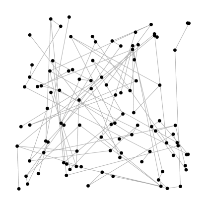
Figure 7: Sample network for $n=100$ nodes.

Problem data.

We model the network as in [KCLB+13] with the same parameters, which results in a network with high local connectivity and a few longer transmission lines. Figure 7 shows an example with $n=100$. We draw the demand $d_{i}$ for each node uniformly at random from the set $\{0.5,1,2\}$. For each transmission line, we set $\alpha_{i}=16$ and $\beta_{i}=1/4$. We draw the maximum capacity for each line uniformly at random from the set $\{1,2,3\}$. These numbers imply that a line with maximum capacity $1$ operating at full capacity will loose about $10\%$ of the power transmitted, whereas a line with maximum capacity $3$ will loose almost $40\%$ of the power transmitted. For the purposes of this example, we let all lines be bidirectional: if there is a line connecting node $j$ to node $j^{\prime}$, we add a line connecting node $j^{\prime}$ to node $j$ with the same parameters.

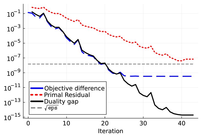
(a) Convergence of ConvexFlows with $n=100$. The objective is compared to a high-precision solution from Mosek. The primal residual measures the net flow constraint violation, with $\{x_{i}\}$ from (14c) and $y$ from (14a).

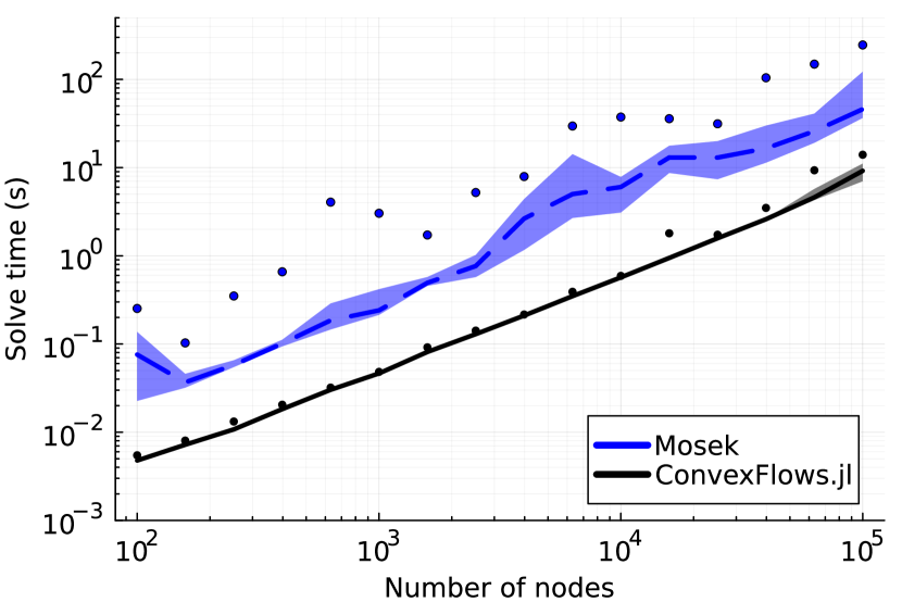
(b) Comparison of ConvexFlows with Mosek. Lines indicate the median time over 10 trials, and the shaded region indicates the 25th to 75th quantile range. Dots indicate the maximum time over the 10 trials.

Figure 8: Numerical results for the optimal power flow problem.

Numerical results.

We first examine the convergence per of our method on an example with $n=100$ nodes and $m=198$ transmission lines. In figure 8(a), we plot the relative duality gap, net flow constraint violation, and difference between our objective value and the ‘optimal’ objective value, obtained using the commercial solver Mosek. (See appendix C.1 for the conic formulation). These results suggest that our method enjoys linear convergence. The difference in objective value at ‘optimality’ is likely due to floating point numerical inaccuracies, as it is below the square root of machine precision, denoted by $\sqrt{\texttt{eps}}$. In figure 8(b), we compare the runtime of our method to Mosek for increasing values of $n$, with ten trials for each value. For each $n$, we plot the median time, the 25th to 75th quantile, and the maximum time. Our method clearly results in a significant and consistent speedup. Notably, our method exhibits less variance in solution time as well. We emphasize, however, that our implementation is not highly optimized and relies on an ‘off-the-shelf’ L-BFGS-B solver. We expect that further software improvement could yield even better performance.

6.2 Routing orders through financial exchanges

Next, we consider a problem which includes both edges connecting more than two nodes and utilities on the edge flows: routing trades through decentralized exchanges (see §3.5). For all experiments, we use the net flow utility function

$$U(y)=c^{T}y-I_{\mathbf{R}_{+}^{n}}(y).$$

We interpret this function as finding arbitrage in the network of markets. More specifically, we wish to find the most valuable trade $y$, measured according to price vector $c$, which, on net, tenders no assets to the network. The associated subproblem (14a) can be computed as

$$\bar{U}(\nu)=\begin{cases}0&\nu\geq c\\ \infty&\text{otherwise}.\end{cases}$$

We also want to ensure our trade with any one market is not too large, so we add a penalty term to the objective:

$$V_{i}(x_{i})=-(1/2)\|(x_{i})_{-}\|_{2}^{2}.$$

(Recall that negative entries denote assets tendered to an exchange.) The associated subproblem is

$$\bar{V}_{i}(\xi)=(1/2)\|\xi\|_{2}^{2}.$$

Finally, the arbitrage problem here is exactly the problem of computing an optimal arbitrage trade with each market, given prices on some infinitely-liquid external market.

Problem data.

We generate $m$ markets and $n=2\sqrt{m}$ assets. We use three popular market implementations for testing: Uniswap (v2) [ZCP18], Balancer [MM19] two-asset markets, and Balancer three-asset markets. We provide the details of these markets and the associated arbitrage problems in appendix C.2. Markets are Uniswap-like with probability $2/5$, Balancer-like two-asset markets with probability $2/5$, and Balancer-like three-asset markets with probability $1/5$. Each market $i$ connects randomly selected assets and has reserves sampled uniformly at random from the interval $[100,\,200]^{n_{i}}$.

(a) Convergence without edge penalties.

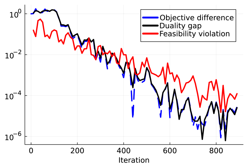
(b) Convergence with edge penalties.

Figure 9: Convergence of ConvexFlows on an example with $n=100$ assets and $m=2500$ markets.

Numerical results.

We first examine the convergence of our method on an example with $m=2500$ and $n=100$. In figures 9(a) and 9(b), we plot the convergence of the relative duality gap, the feasibility violation of $y$, and the relative difference between the current objective value and the optimal objective value, obtained using the commercial solver Mosek. (See appendix C.2 for the conic formulation we used.) Note that, here, we reconstruct $y$ as

$$y=\sum_{i=1}^{m}A_{i}x_{i},$$

instead of using the solution to the subproblem (14a) as we did in the previous example. As a result, this $y$ satisfies the net flow constraint by construction. We measure the feasibility violation relative to the implicit constraint in the objective function $U$, which is that $y\geq 0$. We again see that our method enjoys linear convergence in both cases; however, the convergence is significantly slower when edge objectives are added (figure 9(b)). We then compare the runtime of our method and the commercial solver Mosek, both without edge penalties and with only two-node edges, in figure 10. Again, ConvexFlows enjoys a significant speedup over Mosek.

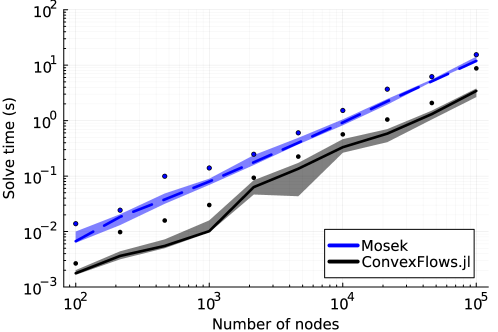
Figure 10: Comparison of ConvexFlows and Mosek for $m$ varying from $100$ to $100,000$ and $n=2\sqrt{m}$. Lines indicate the median time over 10 trials, and the shaded region indicates the 25th to 75th quantile range. Dots indicate the maximum time over the 10 trials.

7 Conclusion

In this paper, we introduced the convex network flow problem, which is a natural generalization of many important problems in computer science, operations research, and related fields. We showed that many problems from the literature are special cases of this framework, including max-flow, optimal power flow, routing through financial markets, and equilibrium computation in Fisher markets, among others. This generalization has a number of useful properties including, and perhaps most importantly, that its dual decomposes over the (hyper)graph structure. This decomposition results in a fast algorithm that easily parallelizes over the edges of the graph and preserves the structure present in the original problem. We implemented this algorithm in the Julia package ConvexFlows.jl and showed order-of-magnitude speedups over a commercial solver applied to the same problem.

Future work.

We believe that analyzing the convex flow problem properties in a more systematic way will lead to several interesting future research directions. For example, we mention in §3.1 that bidirectional edge flows can be viewed as the Minkowski sum of two directional edge flows, one in each direction. Can this idea be generalized to other feasible sets? What does a natural version of this look like? Other important generalizations include: is it possible to extend this framework to include fixed costs for using (or not using) an edge? Does this problem’s dual formulation have a more natural dual that has a similar interpretation as the primal, akin to the self-duality in extended monotropic programming [Ber08]? And, finally, is there an easier-to-use interface for solvers of this particular problem, which does not require specifying solutions to the subproblems (14) directly? We suspect many of these questions are interesting from both a theoretical and practical perspective, given the relevance of this problem formulation to many applications.

Appendix A Extended monotropic programming

In this section, we explicitly draw the connection between the extended monotropic programming (EMP) problem formulated by Bertsekas [Ber08] and the convex flow problem (1). The extended monotropic programming problem can be written as

minimize $$\sum_{i=1}^{m+1}f_{i}(z_{i})$$

subject to $$z\in S,$$

with variable $z\in\mathbf{R}^{N}$. The functions $f_{i}$ are convex functions of the subvectors $z_{i}$, and the set $S$ is a subspace of $\mathbf{R}^{N}$. Taking $z=(y,x_{1},\dots,x_{m})$ and changing the minimization to a maximization, we can write the convex flow problem as a monotropic programming problem:

maximize $$U(y)+\sum_{i=1}^{m}V_{i}(x_{i})-I_{T_{i}}(x_{i})$$

subject to $$y=\sum_{i=1}^{m}A_{i}x_{i},$$

where we took

$$f_{m+1}=-U,\qquad\text{and}\qquad f_{i}=-V_{i}+I_{T_{i}},\quad i=1,\dots,m,$$

Note that the linear net flow constraint is a subspace constraint.

Duality.

The dual of the EMP problem considered by Bertsekas is given by

maximize $$-\sum_{i=1}^{m+1}\sup_{z_{i}\in\mathbf{R}^{n_{i}}}\left\{\lambda_{i}^{T}z_{i}-f_{i}(z_{i})\right\}$$

subject to $$\lambda\in S^{\perp}.$$

Substituting in $U$ and $\{V_{i}\}$ and switching the sign of $\lambda$, the objective terms become

$$\sup_{z_{m+1}\in\mathbf{R}^{n}}\left\{U(z_{m+1})-\lambda_{m+1}^{T}z_{m+1}\right\}=\bar{U}(\lambda_{m+1})\qquad\text{and}\qquad\sup_{z_{i}\in T_{i}}\left\{V_{i}(z_{i})-\lambda_{i}^{T}z_{i}\right\}.$$

These terms are very close to, but not exactly the same as, the dual terms in the convex flow problem (17). In particular, the $U$ subproblem (14a) remains the same, but, in our framework, we introduced an additional dual variable to split the $V_{i}$ subproblem into two subproblems: one for the function $V_{i}$ (14b) and one for the set $T_{i}$ (14c). This split allows for a more efficient algorithm that uses the ‘arbitrage’ primitive (14c), which has a very fast implementation for many edges, especially in the case of two node edges (see §5.1). Our dual problem for the convex flow problem allows us to exploit more structure in our solver.

When the EMP problem matches.

In the case of zero edge utilities, however, the EMP problem matches the convex network flow problem exactly. In this case, the $V$ subproblem disappears and we are left only with the arbitrage subproblem:

$$\sup_{z_{i}\in T_{i}}\left\{V_{i}(z_{i})-\lambda_{i}^{T}z_{i}\right\}=\sup_{z_{i}\in T_{i}}\left\{-\lambda_{i}^{T}z_{i}\right\}=f_{i}(-\lambda_{i}).$$

Letting $\nu=-\lambda_{m}$, the subspace constraint then becomes

$$\lambda_{i}=A_{i}^{T}\nu,\quad i=1,\dots,m.$$

Thus, we recover the exact dual of the convex flow problem with zero edge utilities, given in (21). This immediately implies the strong duality result given in [Ber08, Prop 2.1] holds in our setting as well.

Self duality.

The EMP dual problem has the same form as the primal; in this sense, the EMP problem is self-dual. The convex flow problem, however, does not appear to be self-dual in the same sense, since we consider a very specific subspace that defines the net flow constraint. We leave exploration of duality in our setting to future work.

Appendix B Fisher market problem KKT conditions

The Lagrangian of the Fisher market problem (9) is

$$L(x,\mu,\lambda)=\sum_{i=1}^{n_{b}}b_{i}\log(U(x_{i}))+\mu^{T}\left(\mathbf{1}-\sum_{i=1}^{n_{b}}x_{i}\right)-\sum_{i=1}^{n_{b}}x_{i}^{T}\lambda_{i},$$

where $\{x_{i}\in\mathbf{R}^{n_{g}}\}$ are the primal variables and $\mu\in\mathbf{R}^{n_{g}}$ and $\{\lambda_{i}\in\mathbf{R}_{+}^{n_{g}}\}$ are the dual variables. Let $x^{\star}$, $\mu^{\star}$, $\lambda^{\star}$ be a primal-dual solution to this problem. The optimality conditions [BV04, §5.5] are primal feasibility, complementary slackness, and the dual condition

$$\partial_{x_{i}}L(x^{\star},\mu^{\star},\lambda^{\star})=\frac{b_{i}}{U(x_{i}^{\star})}\nabla U(x_{i}^{\star})-\mu^{\star}-\lambda^{\star}_{i}=0,\quad\text{for}~{}i=1,\dots,n_{b}.$$

This condition simplifies to

$$\nabla U(x_{i}^{\star})\geq(U(x_{i})/b_{i})\cdot\mu^{\star},\quad\text{for}~{}i=1,\dots,n_{b}.$$

If we let the prices of the goods be $\mu^{\star}\in\mathbf{R}^{n_{g}}$, this condition says that the marginal utility gained by an agent $i$ from an additional small amount of any good is at least as large as that agent’s budget-weighted price times their current utility. As a result, the prices $\mu^{\star}$ will cause all agents to spend their entire budget on a utility-maximizing basket of goods, and all goods will be sold.

Appendix C Additional details for the numerical experiments

C.1 Optimal power flow

Arbitrage problem.

Here, we explicitly work out the arbitrage subproblem for the optimal power flow problem. Recall that the set of allowable flows is given by (dropping the edge index for convenience)

$$T=\{z\in\mathbf{R}^{2}\mid-b\leq z_{1}\leq 0~{}z_{2}\leq-z_{1}-\ell(-z_{1})\},$$

where

$$\ell(w)=16\left(\log(1+\exp(w/4))-\log 2\right)-2w$$

Given an edge input $w\in[0,b]$, the gain function is

$$h(w)=w-\ell(w),$$

where we assume the edge capacity $b$ is chosen such that the function $f$ is increasing for all $w\in[0,b]$, i.e., $f^{\prime}(b)>0$. Using (27), we can compute the optimal solution $x^{\star}$ to the arbitrage subproblem (14c) as

$$x^{\star}_{1}=\left(4\log\left(\frac{3\eta_{2}-\eta_{1}}{\eta_{2}+\eta_{1}}\right)\right)_{[0,b]},\qquad x^{\star}_{2}=h(x^{\star}_{1}),$$

where $(\cdot)_{[0,b]}$ denotes the projection onto the interval $[0,b]$.

Conic formulation.

Define the exponential cone as

$$K_{\mathrm{exp}}=\{(x,y,z)\in\mathbf{R}^{3}\mid y>0,\;ye^{x/y}\leq z.\}$$

The transmission line constraint is of the form

$$\log(1+e^{s})\leq t,$$

which can be written as [ApS24, §5.2.5]

$$u+v \leq 1$$

$$(x-t,\,1,\,u) \in K_{\mathrm{exp}}$$

$$(-t,\,1,\,v) \in K_{\mathrm{exp}}.$$

Define the rotated second order cone as

$$K_{\mathrm{rot2}}=\{(t,u,x)\in\mathbf{R}_{+}\times\mathbf{R}_{+}\times\mathbf{R}^{n}\mid 2tu\geq\|x\|_{2}^{2}\}.$$

We can write the cost function

$$c_{i}(w)=(1/2)w_{+}^{2},$$

where $w_{+}=\max(w,0)$ denotes the negative part of $w$, in conic form as minimizing $t_{1}\in\mathbf{R}$ subject to the second-order cone constraint [ApS24, §3.2.2]

$$(0.5,\,t_{1},\,t_{2})\in K_{\mathrm{rot2}},\qquad t_{2}\geq w,\qquad t_{2}\geq 0.$$

Putting this together, the conic form problem is

maximize $$-\mathbf{1}^{T}t_{1}$$

subject to $$(0.5,\,(t_{1})_{i},\,(t_{2})_{i})\in K_{\mathrm{rot2}},\quad\text{for}~{}i=1,\dots n$$

$$t_{2}\geq d-y,\qquad t_{2}\geq 0$$

$$-b_{i}\leq(x_{i})_{1}\leq 0,\quad\text{for}~{}i=1,\dots m$$

$$u_{i}+v_{i}\leq 1\quad\text{for}~{}i=1,\dots m$$

$$\left(-\beta_{i}(x_{i})_{1}+(3(x_{i})_{1}+(x_{i})_{2})/\alpha-\log(2),\,1,\,u_{i}\right)\in K_{\mathrm{exp}}\quad\text{for}~{}i=1,\dots m$$

$$\left((3(x_{i})_{1}+(x_{i})_{2})/\alpha-\log(2),\,1,\,v_{i}\right)\in K_{\mathrm{exp}}\quad\text{for}~{}i=1,\dots m.$$

C.2 Routing orders through financial exchanges

In this example, we considered three different types of decentralized exchange markets: Uniswap-like, Balancer-like swap markets, and Balancer-like multi-asset markets. Recall that a constant function market maker (CFMM) allows trades between the $n$ tokens in its reserves $R\in\mathbf{R}^{n}_{+}$ with behavior governed by a trading function $\varphi:\mathbf{R}^{n}_{+}\to\mathbf{R}$. The CFMM only accepts a trade $(\Delta,\Lambda)$ where $\Delta\in\mathbf{R}^{n}_{+}$ is the basket of tendered tokens and $\Lambda\in\mathbf{R}^{n}_{+}$ is the basket of received tokens if

$$\varphi(R+\gamma\Delta-\Lambda)\geq\varphi(R).$$

The Uniswap trading function $\varphi_{\mathrm{Uni}}:\mathbf{R}^{2}_{+}\to\mathbf{R}$ is given by

$$\varphi_{\mathrm{Uni}}(R)=\sqrt{R_{1}R_{2}}.$$

The Balancer swap market trading function $\varphi_{\mathrm{Bal}}:\mathbf{R}^{2}_{+}\to\mathbf{R}$ is given by

$$\varphi_{\mathrm{Bal}}(R)=R_{1}^{4/5}R_{2}^{1/5}.$$

The Balancer multi-asset trading function $\varphi_{\mathrm{Mul}}:\mathbf{R}^{3}_{+}\to\mathbf{R}$ is given by

$$\varphi_{\mathrm{Mul}}(R)=R_{1}^{1/3}R_{2}^{1/3}R_{3}^{1/3}.$$

These functions are easily recognized as (weighted) geometric means and can be verified as concave, nondecreasing function. Thus, the set of allowable trades

$$T=\{\Lambda-\Delta\mid\Lambda,\Delta\in\mathbf{R}^{n}_{+}~{}\text{and}~{}\varphi(R+\gamma\Delta-\Lambda)\geq\varphi(R)\},$$

is convex. Furthermore, the arbitrage problem (14c) has a closed form solution for the case of the swap markets (see [AKCNC20, App. A] and the implementation from [DRCA23]).

CFMMs as conic constraints.

Define the power cone as

$$K_{\mathrm{pow}}(w)=\{(x,y,z)\in\mathbf{R}^{3}:x^{w}y^{1-w}\geq|z|,x\geq 0,y\geq 0\}.$$

We model the two-asset market constraints as

$$\begin{bmatrix}R+\gamma\Delta-\Lambda;&\varphi(R)\end{bmatrix}\in K_{\mathrm{pow}}(w),\qquad\text{and}\qquad\Delta,\Lambda\geq 0$$ (30)

where $w=0.5$ for Uniswap and $w=0.8$ for Balancer. Define the geometric mean cone as

$$K_{\mathrm{geomean}}=\left\{(t,x)\in\mathbf{R}^{n+1}:x\geq 0,t\leq\left(x_{1}x_{2}\cdots x_{n}\right)^{1/n}\right\}$$

We model the multi-asset market constraint as

$$\begin{bmatrix}-3\varphi(R);R+\gamma\Delta-\Lambda\end{bmatrix}\in K_{\mathrm{geomean}}\qquad\text{and}\qquad\Delta,\Lambda\geq 0$$ (31)

Objectives as conic constraints.

Define the rotated second order cone as

$$K_{\mathrm{rot2}}=\{(t,u,x)\in\mathbf{R}_{+}\times\mathbf{R}_{+}\times\mathbf{R}^{n}\mid 2tu\geq\|x\|_{2}^{2}\}.$$

The net flow utility function is

$$U(y)=c^{T}y-(1/2)\sum_{i=1}^{n}(y_{i})_{-}^{2},$$

where $x_{-}=\max(-x,0)$ denotes the negative part of $x$. In conic form, maximizing $U$ is equivalent to maximizing

$$c^{T}y-(1/2)\sum_{i=1}^{n}(p_{1})_{i}$$

subject to the constraints

$$p_{2}\geq 0,\qquad p_{2}\geq-y,\qquad(p_{1})_{i},(p_{2})_{i})\in K_{\mathrm{rot2}}\quad\text{for}~{}i=1,\dots,n,$$

where we introduced new variables $p_{1},p_{2}\in\mathbf{R}^{n}$ [ApS24, §3.2.2]. The $V_{i}$’s can be modeled similarly using the rotated second order cone.

Conic form problem.

The CFMM arbitrage example can then be written in conic form as

maximize $$c^{T}y-(1/2)\sum_{i=1}^{n}(p_{1})_{i}-(1/2)\sum_{i=1}^{m}(t_{1})_{i}$$

subject to $$(0.5,(p_{1})_{i},(p_{2})_{i})\in K_{\mathrm{rot2}},\quad i=1,\dots,n$$

$$p_{1}\geq 0$$

$$p_{2}\geq 0,\quad p_{2}\geq-y$$

$$(0.5,(t_{1})_{i},(t_{2})_{i})\in K_{\mathrm{rot2}},\quad i=1,\dots,n$$

$$t_{1}\geq 0$$

$$t_{2}\geq 0,\quad(t_{2})_{i}\geq-(\Lambda_{i}-\Delta_{i})$$

$$\begin{bmatrix}R+\gamma\Delta-\Lambda;&\varphi(R)\end{bmatrix}\in K_{\mathrm{pow}}(w_{i}),\quad i=1,\dots,m_{1}$$

$$\begin{bmatrix}-3\varphi(R);&R+\gamma\Delta-\Lambda\end{bmatrix}\in K_{\mathrm{geomean}},\quad i=m_{1}+1,\dots,m$$

$$\Delta_{i},\;\Lambda_{i}\geq 0,\quad i=1,\dots,m,$$

with variables $y\in\mathbf{R}^{n}$, $p_{1}\in\mathbf{R}^{n}$, $p_{2}\in\mathbf{R}^{n}$, $t_{1}\in\mathbf{R}^{m}$, $(t_{2})_{i}\in\mathbf{R}^{n_{i}}$, $\Delta\in\mathbf{R}^{n_{i}}$, and $\Lambda\in\mathbf{R}^{n_{i}}$ for $i=1,\dots,m$.

References

- [AAECB22] Guillermo Angeris, Akshay Agrawal, Alex Evans, Tarun Chitra and Stephen Boyd “Constant Function Market Makers: Multi-asset Trades via Convex Optimization” In Handbook on Blockchain Cham: Springer International Publishing, 2022, pp. 415–444 DOI: 10.1007/978-3-031-07535-3˙13
- [ABNKZ22] Akshay Agrawal, Stephen Boyd, Deepak Narayanan, Fiodar Kazhamiaka and Matei Zaharia “Allocation of fungible resources via a fast, scalable price discovery method” In Mathematical Programming Computation 14.3 Springer, 2022, pp. 593–622
- [AC20] Guillermo Angeris and Tarun Chitra “Improved Price Oracles: Constant Function Market Makers” In Proceedings of the 2nd ACM Conference on Advances in Financial Technologies New York NY USA: ACM, 2020, pp. 80–91 DOI: 10.1145/3419614.3423251
- [ACDEK23] Guillermo Angeris, Tarun Chitra, Theo Diamandis, Alex Evans and Kshitij Kulkarni “The geometry of constant function market makers” In arXiv preprint arXiv:2308.08066, 2023
- [AECB22] Guillermo Angeris, Alex Evans, Tarun Chitra and Stephen Boyd “Optimal routing for constant function market makers” In Proceedings of the 23rd ACM Conference on Economics and Computation, 2022, pp. 115–128
- [AKCNC20] Guillermo Angeris, Hsien-Tang Kao, Rei Chiang, Charlie Noyes and Tarun Chitra “An Analysis of Uniswap Markets” In Cryptoeconomic Systems, 2020 DOI: 10.21428/58320208.c9738e64
- [AMO88] Ravindra K Ahuja, Thomas L Magnanti and James B Orlin “Network flows” Cambridge, Mass.: Alfred P. Sloan School of Management, Massachusetts, 1988
- [ApS24] Mosek ApS “MOSEK Modeling Cookbook”, 2024
- [ApS24a] MOSEK ApS “MOSEK Optimizer API for Julia”, 2024 URL: https://docs.mosek.com/10.1/juliaapi/index.html
- [AZR20] Hayden Adams, Noah Zinsmeister and Dan Robinson “Uniswap v2 Core” In URL: https://uniswap.org/whitepaper.pdf, 2020
- [BEKS17] Jeff Bezanson, Alan Edelman, Stefan Karpinski and Viral Shah “Julia: A Fresh Approach to Numerical Computing” In SIAM Review 59.1, 2017, pp. 65–98 DOI: 10.1137/141000671
- [Ber08] Dimitri P Bertsekas “Extended monotropic programming and duality” In Journal of optimization theory and applications 139.2 Springer, 2008, pp. 209–225
- [Ber15] Dimitri Bertsekas “Convex optimization algorithms” Athena Scientific, 2015
- [Ber16] Dimitri Bertsekas “Nonlinear Programming” Belmont, Massachusetts: Athena Scientific, 2016
- [Ber98] Dimitri Bertsekas “Network optimization: continuous and discrete models” Athena Scientific, 1998
- [BG92] Dimitri Bertsekas and Robert Gallager “Data networks” Athena Scientific, 1992
- [BLNZ95] Richard H Byrd, Peihuang Lu, Jorge Nocedal and Ciyou Zhu “A limited memory algorithm for bound constrained optimization” In SIAM Journal on scientific computing 16.5 SIAM, 1995, pp. 1190–1208
- [BV04] Stephen Boyd and Lieven Vandenberghe “Convex Optimization” Cambridge, United Kingdom: Cambridge University Press, 2004
- [BXMM07] Stephen Boyd, Lin Xiao, Almir Mutapcic and Jacob Mattingley “Notes on decomposition methods” In Notes for EE364B, Stanford University 635 Citeseer, 2007, pp. 1–36
- [CKV21] Chris Coey, Lea Kapelevich and Juan Pablo Vielma “Solving natural conic formulations with Hypatia.jl”, 2021 arXiv:2005.01136 [math.OC]
- [CLCD07] Mung Chiang, Steven H Low, A Robert Calderbank and John C Doyle “Layering as optimization decomposition: A mathematical theory of network architectures” In Proceedings of the IEEE 95.1 IEEE, 2007, pp. 255–312
- [DF56] George Bernard Dantzig and Delbert R Fulkerson “On the Max-Flow Min-Cut Theorem of Networks” Princeton university press, 1956, pp. 215–222
- [DHL17] Iain Dunning, Joey Huchette and Miles Lubin “JuMP: A Modeling Language for Mathematical Optimization” In SIAM Review 59.2, 2017, pp. 295–320 DOI: 10.1137/15M1020575
- [DRCA23] Theo Diamandis, Max Resnick, Tarun Chitra and Guillermo Angeris “An Efficient Algorithm for Optimal Routing Through Constant Function Market Makers” In arXiv preprint arXiv:2302.04938, 2023
- [EFS56] Peter Elias, Amiel Feinstein and Claude Shannon “A note on the maximum flow through a network” In IRE Transactions on Information Theory 2.4 IEEE, 1956, pp. 117–119
- [EG59] Edmund Eisenberg and David Gale “Consensus of subjective probabilities: The pari-mutuel method” In The Annals of Mathematical Statistics 30.1 JSTOR, 1959, pp. 165–168
- [Ego19] Michael Egorov “Stableswap-efficient mechanism for stablecoin liquidity”, 2019
- [FF56] Lester Randolph Ford and Delbert R Fulkerson “Maximal flow through a network” In Canadian journal of Mathematics 8 Cambridge University Press, 1956, pp. 399–404
- [FF57] Lester Randolph Ford and Delbert R Fulkerson “A simple algorithm for finding maximal network flows and an application to the Hitchcock problem” In Canadian journal of Mathematics 9 Cambridge University Press, 1957, pp. 210–218
- [HR55] TE Harris and FS Ross “Fundamentals of a method for evaluating rail net capacities”, 1955
- [KCLB+13] Matt Kraning, Eric Chu, Javad Lavaei and Stephen Boyd “Dynamic network energy management via proximal message passing” In Foundations and Trends® in Optimization 1.2 Now Publishers, Inc., 2013, pp. 73–126
- [Kuh55] Harold W Kuhn “The Hungarian method for the assignment problem” In Naval research logistics quarterly 2.1-2 Wiley Online Library, 1955, pp. 83–97
- [LDDHLV23] Miles Lubin, Oscar Dowson, Joaquim Dias Garcia, Joey Huchette, Benoît Legat and Juan Pablo Vielma “JuMP 1.0: Recent improvements to a modeling language for mathematical optimization” In Mathematical Programming Computation, 2023 DOI: 10.1007/s12532-023-00239-3
- [LDGL21] Benoît Legat, Oscar Dowson, Joaquim Garcia and Miles Lubin “MathOptInterface: A Data Structure for Mathematical Optimization Problems” In INFORMS Journal on Computing, 2021, pp. ijoc.2021.1067 DOI: 10.1287/ijoc.2021.1067
- [MM19] Fernando Martinelli and Nikolai Mushegian “Balancer: A Non-Custodial Portfolio Manager, Liquidity Provider, and Price Sensor”, 2019
- [MN11] José Luis Morales and Jorge Nocedal “Remark on “Algorithm 778: L-BFGS-B: Fortran subroutines for large-scale bound constrained optimization”” In ACM Transactions on Mathematical Software (TOMS) 38.1 ACM New York, NY, USA, 2011, pp. 1–4
- [NB22] Anna Nagurney and Deniz Besik “Spatial price equilibrium networks with flow-dependent arc multipliers” In Optimization Letters 16.8 Springer, 2022, pp. 2483–2500
- [OCPB16] Brendan O’Donoghue, Eric Chu, Neal Parikh and Stephen Boyd “Conic Optimization via Operator Splitting and Homogeneous Self-Dual Embedding” In Journal of Optimization Theory and Applications 169.3, 2016, pp. 1042–1068 DOI: 10.1007/s10957-016-0892-3
- [Roc70] R. Tyrrell Rockafellar “Convex Analysis” Princeton university press, 1970
- [Roc84] RT Rockafellar “Network flows and monotropic programming” In Witey-Interscience: New York, 1984
- [Rou07] Tim Roughgarden “Routing games” In Algorithmic game theory 18 Cambridge University Press Cambridge, 2007, pp. 459–484
- [Sch02] Alexander Schrijver “On the history of the transportation and maximum flow problems” In Mathematical programming 91 Springer, 2002, pp. 437–445
- [Sha48] Claude Elwood Shannon “A mathematical theory of communication” In The Bell system technical journal 27.3 Nokia Bell Labs, 1948, pp. 379–423
- [Shi06] Maiko Shigeno “Maximum network flows with concave gains” In Mathematical programming 107.3 Springer, 2006, pp. 439–459
- [STA09] Peter Schütz, Asgeir Tomasgard and Shabbir Ahmed “Supply chain design under uncertainty using sample average approximation and dual decomposition” In European journal of operational research 199.2 Elsevier, 2009, pp. 409–419
- [Stu19] Paul Melvin Stursberg “On the mathematics of energy system optimization”, 2019
- [Tru78] Klaus Truemper “Optimal flows in nonlinear gain networks” In Networks 8.1 Wiley Online Library, 1978, pp. 17–36
- [Vaz07] Vijay V Vazirani “Combinatorial algorithms for market equilibria” In Algorithmic game theory, 2007, pp. 103–134
- [Vaz12] Vijay V Vazirani “The notion of a rational convex program, and an algorithm for the Arrow-Debreu Nash bargaining game” In Journal of the ACM (JACM) 59.2 ACM New York, NY, USA, 2012, pp. 1–36
- [Vég14] László A Végh “Concave generalized flows with applications to market equilibria” In Mathematics of Operations Research 39.2 INFORMS, 2014, pp. 573–596
- [Wil19] David P Williamson “Network flow algorithms” Cambridge University Press, 2019
- [WWS13] Allen J Wood, Bruce F Wollenberg and Gerald B Sheblé “Power generation, operation, and control” John Wiley & Sons, 2013
- [XJB04] Lin Xiao, Mikael Johansson and Stephen P Boyd “Simultaneous routing and resource allocation via dual decomposition” In IEEE Transactions on Communications 52.7 IEEE, 2004, pp. 1136–1144
- [ZBLN97] Ciyou Zhu, Richard H Byrd, Peihuang Lu and Jorge Nocedal “Algorithm 778: L-BFGS-B: Fortran subroutines for large-scale bound-constrained optimization” In ACM Transactions on mathematical software (TOMS) 23.4 ACM New York, NY, USA, 1997, pp. 550–560
- [ZCP18] Yi Zhang, Xiaohong Chen and Daejun Park “Formal Specification of Constant Product (Xy=k) Market Maker Model and Implementation”, 2018