Communicating Multiverses in Holographic
de-Sitter Braneworld

Gopal Yadav

Chennai Mathematical Institute,
H1 SIPCOT IT Park, Siruseri 603103, India

In this paper, we construct the wedge holography for the de-Sitter space a bulk theory. First, we discuss a more general mathematical construction of wedge holography in parallel with wedge holography construction for the AdS bulk, and then we construct the wedge holography in the extended static patch. In the first case, we prove that one can construct wedge holography for the de-Sitter bulk for the static patch as well as global coordinate metric on end-of-the-world branes. Extended static patch wedge holography is constructed by joining the two copies of double holography in DS/dS correspondence. We find that wedge holography with extended static patch metric leads to the emergence of communicating universes. Further, we propose a model which provides the theoretical evidence of communicating multiverses.

One day there may well be proof of multiple universes…and in that universe, Zayn is still in one direction.              Stephen Hawking

1 Introduction

It has always been fascinating to question whether our universe is the only universe, whether there are other universes in nature, or whether many universes exist in a multiverse. Is our universe part of a multiverse? Some questions related to Multiverse have been explored in [5, 2, 1, 4, 3]. There is also progress done in this direction within braneworld by the use of wedge holography [6, 7] where the bulk theory is anti de-Sitter spacetime which has negative cosmological constant. In this work, we explore this type of question from the perspective of wedge holography where the bulk is de-Sitter space with positive cosmological constant.

Holography has played an important role in understanding various phenomena in many branches of physics. Originally, it was started as a duality between ${\cal N}$=4 supersymmetric Yang-Mills theory and type IIB string theory on $AdS_{5}\times S^{5}$ background [8]. We are able to decode the information about boundary theory from the bulk theory using holography and vice-versa. There are many generalizations of holography, e.g., dS/CFT correspondence [9, 10] which is a duality between de-Sitter space in bulk and Euclidean CFT living at the future/past boundary of de-Sitter space. This is a co-dimension one holography. In this paper, we discuss co-dimension two holography in the context of de-Sitter space. There is also so-called DS/dS correspondence [11] which describes duality between $d$-dimensional de-Sitter space and two CFTs which are coupled to each other and ($d-1$)-dimensional de-Sitter gravity. Further, see [12, 13, 14] for the application of holography to thermal QCD from a top-down approach, [15, 16] for condensed matter physics, [17, 18, 19] where holography has been used in cosmology, [20, 21, 22] for the discussion on multi-boundary wormholes. There is also a new version of holography in the context of AdS/CFT where time is emergent dimension known as “Cauchy slice holography” [23].

As an application of holography, we are able to resolve the information paradox [24]. For this purpose, there are three proposals: island proposal [25, 26], double holography [27, 28, 29], and wedge holography [30, 31]. In double holography, we couple the black hole living on an end-of-the-world brane with an external CFT bath living at the conformal boundary of the AdS bulk. This external bath acts as a sink to collect the Hawking radiation. Using double holography, the Page curve [32] has been obtained by computing the areas of Hartman-Maldacena [33] and island surfaces. Further, efforts have been made to collect the Hawking radiation in a gravitating bath, and the setup is obtained by introducing two Karch-Randall branes in which one brane acts as a black hole, whereas another brane acts as a bath. The setup with two gravitating branes is known as wedge holography [30, 31].

Wedge holography is a co-dimension two holography, which can be understood as follows. First, we localize the $d$-dimensional bulk Einstein gravity on $(d-1)$-dimensional Karch-Randall branes, which is called as braneworld holography [34, 35] and then the gravity living on Karch-Randall branes is dual to the CFT living at the $(d-2)$-dimensional defect because of AdS/CFT correspondence [8]. Hence, $d$-dimensional Einstein gravity living in the wedge formed by Karch-Randall branes is dual to $(d-2)$-dimensional defect CFT. For the AdS bulk, wedge holography has been explored in detail in [36, 40, 43, 42, 47, 46, 45, 41, 44, 37, 38, 39] and for flat spacetime bulk, see [48]. An interesting application of wedge holography is that it describes multiverse [6, 7] but in the AdS bulk spacetime. The multiverse is obtained by $2n$ Karch-Randall branes, which are joined at the common defect. Since there is Einstein gravity on each branch, therefore, we obtain a Multiverse made up of $2n$ universes [6].

Wedge holography has been successfully constructed in the AdS and flat spacetime bulk. The motivation of the paper is to construct the wedge holography for the de-Sitter bulk. We will see that it is possible to construct wedge holography even for the de-Sitter bulk. This setup provides interesting results. It gives a hint for dS_d/CFT_d-2 correspondence, the existence of communicating universes, multiverse, and communicating multiverses within braneworld.

The rest of the paper is organized as follows. We start with the construction of wedge holography for the de-Sitter bulk in section 2 via three subsections 2.1, 2.2 and 2.3. In subsection 2.1, we describe the mathematical description of de-Sitter wedge holography; in subsection 2.2, we prove that we have consistent wedge holographic realization for the de-Sitter bulk, and in subsection 2.3, we describe de-Sitter wedge holography pictorially. We construct the wedge holography in an extended static patch in section 3 and use this model to discuss whether parallel universes exist or not in section 4. In section 5, we discuss the existence of multiverse (subsection 5.1) and communicating multiverses (subsection 5.2) and then discuss our results in section 6.

2 Wedge holography for the de-Sitter bulk: general description

In this section, we construct wedge holography for the general de-Sitter bulk and prove that the metric on the end-of-the-world branes can be static patch and global coordinate. We consider dimensionality of de-Sitter bulk as $d$-dimensions whereas dimensionality of end-of-the-world branes [located at $\omega=\omega_{1}$ and $\omega=\omega_{2}$] as $(d-1)$-dimensions. The discussion in this section will be general, similar to wedge holography construction for the AdS bulk.

2.1 The setup

The bulk gravitational action with positive cosmological constant in $d$-dimensions including the gravitational action on the branes is given as [49]

$$S=\frac{1}{16\pi G_{N}^{(d)}}\int d^{d}x\sqrt{-g}{\left({\cal R}-2\Lambda\right)}-\frac{1}{8\pi G_{N}^{(d)}}\int d^{d-1}x\sqrt{-\hat{g}_{\beta}}\left({\cal K}_{\beta}-T_{\beta}\right),$$ (1)

where $\beta=1,2$ and $\Lambda=\frac{(d-1)(d-2)}{2}$. $G_{N}^{(d)}$, ${\cal R}$ and $\Lambda$ are the Newton constant, Ricci scalar and cosmological constant in $d$-dimensions; ${\cal K}_{\beta}$ and $T_{\beta}$ are the trace of extrinsic curvature and tensions of end-of-the-world branes. Einstein equation associated with the bulk metric is given by

$$R_{\mu\nu}-\frac{R}{2}g_{\mu\nu}{\bf+}\Lambda g_{\mu\nu}=0.$$ (2)

The above equation has the following solution [11]

$$ds^{2}=d\omega^{2}+e^{2A(\omega)}\hat{g}_{ij}dy^{i}dy^{j},$$ (3)

where $\hat{g}_{ij}$ corresponds to the metric of dS_d-1 space. Depending upon the warp factor, the bulk metric (3) can be either de-Sitter or anti de-Sitter as follows [11]

$${\bf dS_{d}}:\ \ \ \ \ \ \ \ \ e^{2A(\omega)}=\sin^{2}\left(\omega/R\right),$$

$${\bf AdS_{d}}:\ \ \ \ \ \ \ e^{2A(\omega)}=\sinh^{2}\left(\omega/R\right),$$ (5)

where $R$ is the length scale associated with corresponding background. Since we are interested in constructing wedge holography for the de-Sitter bulk, we will consider the de-Sitter case here. Let us write the explicit metric for the de-Sitter bulk as

$$ds_{\rm general\ bulk}^{2}=d\omega^{2}+\sin^{2}\left(\omega/R\right)\hat{g}_{ij}^{\beta}dy^{i}dy^{j},$$

$$ds_{\rm static\ patch}^{2}=d\omega^{2}+\sin^{2}\left(\omega/R\right)\left[-(1-r^{2})dt^{2}+\frac{dr^{2}}{1-r^{2}}+r^{2}d\Omega_{d-3}^{2}\right],$$

$$ds_{\rm global\ de-Sitter}^{2}=d\omega^{2}+\sin^{2}\left(\omega/R\right)\left[-d\tau^{2}+\cosh^{2}\left(\tau\right)d\Omega_{d-2}^{2}\right],$$ (6)

where $t\in(-\infty,\infty)$, $r\in(0,1)$, $\tau\in(-\infty,\infty)$, and
$d\Omega_{d-2}^{2}=d\theta_{1}^{2}+\sin^{2}\theta_{1}d\theta_{2}^{2}+......+\sin^{2}\theta_{1}\sin^{2}\theta_{2}......\sin^{2}\theta_{d-3}d\theta_{d-2}^{2}$.

The Neumann boundary condition (NBC) satisfied by the bulk metric (3) at the location of end-of-the-world branes is given as

$${\cal K}_{ij}^{\beta}-({\cal K}^{\beta}-T^{\beta})\hat{g}_{ij}^{\beta}=0,$$ (7)

where ${\cal K}_{ij}^{\beta}=\frac{1}{2}\partial_{\omega}{\hat{g}_{ij}^{\beta}}|_{\omega=\omega_{1,2}}$ and ${\cal K}^{\beta}=\hat{g}^{ij,\beta}{\cal K}_{ij,\beta}$.

It has been discussed in [11] that the de-Sitter bulk (2.1) is dual to two CFTs on $dS_{d-1}$ which are coupled to each other and $(d-1)$-dimensional de-Sitter gravity at $\omega=\frac{\pi R}{2}$. The warp factor is maximum at $\omega=\frac{\pi R}{2}$ and it is zero at the horizon, $\omega=0,\pi R$. For the discussion in this section, we will consider localization of $d$-dimensional de-Sitter gravity on $(d-1)$-dimensional EOW brane [50].

Having discussed the general structure of $d$-dimensional de-Sitter space, let us see how we can construct wedge holography in de-Sitter space. Let us consider two EOW branes located at $\omega=\omega_{1}$ and $\omega=\omega_{2}$ which are basically constant $\omega$ slicing of the bulk metric (2.1). It is to be noted that the story here is different from the AdS bulk because wedge holography construction of de-Sitter bulk is a little bit difficult. We will discuss this pictorially in subsection 2.3 using the idea of [51]. For now, we are considering EOW branes at some arbitrary locations $\omega_{1,2}$. The wedge holography is obtained by joining two $(d-1)$-dimensional EOW branes (say $Y_{1}$ and $Y_{2}$) with de-Sitter metric at the $(d-2)$-dimensional defect in $d$-dimensional de-Sitter bulk (see Fig. 1).

Similar to AdS and flat bulk spacetime, we expect that de-Sitter wedge holography has the following three descriptions:

• Boundary description: $(d-2)$-dimensional defect CFT living at the corner of the wedge formed by two EOW branes.

• Intermediate description: the gravitating branes ($Y_{1}$ and $Y_{2}$) with metric $dS_{d-1}$ are interacting with each other via the transparent boundary conditions at the defect.

• Bulk description: CFT living on the $(d-2)$-dimensional defect is dual to $d$-dimensional de-Sitter gravity living in the wedge formed by gravitating EOW branes with metric dS_d-1.

When we take de-Sitter slicing of (3) then we expect that defect CFT should be non-unitary because of dS/CFT correspondence [9, 10]. Let us make statement about the wedge holography [30, 31] in the context of de-Sitter bulk as follows:

Classical gravity in $d$-dimensional de-Sitter space
$\equiv$ (Quantum) gravity on two $(d-1)$-dimensional EOW branes with metric dS_d-1
$\equiv$ CFT living at the $(d-2)$-dimensional defect.

The first and the second lines are related via braneworld holography in de-Sitter space [50] whereas the second and third lines exist because of dS/CFT correspondence [9, 10]. Hence, classical gravity in $d$-dimensional de-Sitter space is dual to $(d-2)$-dimensional defect CFT living at the corner of the wedge, which is the signature of dS_d/CFT_d-2 correspondence.

To get a consistent wedge holographic realization of the de-Sitter space, we need to check the following conditions:

1. The bulk metric (2.1) should satisfy Einstein’s equation with a positive cosmological constant (2).

2. The bulk metric (2.1) must satisfy Neumann boundary conditions (7) on the branes, i.e. at $\omega=\omega_{1,2}$ where $\omega_{1,2}$ are some constant values of $\omega$.

3. The induced metric $\hat{g}_{ij}^{\beta}$ on the branes should be the solution of Einstein’s equation with a positive cosmological constant in $(d-1)$-dimensions:

   $$R_{ij}^{\beta}-\frac{1}{2}\hat{g}_{ij}^{\beta}R[\hat{g}_{ij}^{\beta}]+\frac{(d-2)(d-3)}{2}\hat{g}_{ij}^{\beta}=0.$$ (8)

One can obtain the gravitational action on the branes from the substitution of (2.1) into the bulk action (1), using the Neumann boundary condition (7) and integration over $\omega$ and the general form is given as

$$S_{\rm brane}=\lambda_{\beta}^{\rm dS}\int d^{d-1}x\left(R[\hat{g}_{ij}^{\beta}]-2\Lambda_{\rm brane}^{\rm dS}\right),$$ (9)

where $\Lambda_{\rm brane}^{\rm dS}=\frac{(d-2)(d-3)}{2}$, $\lambda_{\beta}^{\rm dS}=\frac{1}{16\pi G_{N}^{(d-1),\beta}}$. Here, we show that condition 2 is satisfied, provided EOW branes have some tensions. Let us see this in more detail. For the bulk metric (2.1), extrinsic curvature and the trace of the same on EOW branes are obtained as

$${\cal K}_{ij}^{\beta}=\frac{1}{2}\partial_{\omega}{\hat{g}_{ij}}|_{\omega=\omega_{1,2}}=\frac{1}{R}\cot\left(\frac{\omega_{1,2}}{R}\right)\hat{g}_{ij}|_{\omega=\omega_{1,2}},$$

$${\cal K}^{\beta}=\hat{g}^{ij,\beta}{\cal K}_{ij}^{\beta}=\frac{d-1}{R}\cot\left(\frac{\omega_{1,2}}{R}\right).$$ (10)

Hence, using the Neumann boundary condition (7) and the information given in (2.1), we see that NBC for the bulk metric (2.1) is satisfied when tensions of the branes are given by

$$T^{\beta}=\frac{d-2}{R}\cot\left(\frac{\omega_{1,2}}{R}\right).$$ (11)

Hence at $\omega_{1,2}=\frac{\pi R}{2}$, we get tensionless branes as discussed in [49].

2.2 Wedge holography in various dimensions

In this subsection, we construct wedge holography for various dimensional de-Sitter bulk. For simplicity, we work with $R=1$ unit.

2.2.1 $d=3$

For three-dimensional de-Sitter space, the bulk metric is given as

$$ds^{2}=d\omega^{2}+\sin^{2}\left(\omega\right)\hat{g}_{ij}^{\beta}dy^{i}dy^{j},$$

$$ds_{\rm static\ patch}^{2}=d\omega^{2}+\sin^{2}\left(\omega\right)\left[-(1-r^{2})dt^{2}+\frac{dr^{2}}{1-r^{2}}\right],$$

$$ds_{\rm global\ de-Sitter}^{2}=d\omega^{2}+\sin^{2}\left(\omega\right)\left[-d\tau^{2}+\cosh^{2}\left(\tau\right)d\Omega_{1}^{2}\right],$$ (12)

where $d\Omega_{1}^{2}=d\theta_{1}^{2}$. For this case, the Ricci scalar is $R=6$, and the Ricci tensors for the static patch and global de-Sitter are summarized below.

• Ricci tensors for static patch:

  $$R_{11}=2\left(r^{2}-1\right)\sin^{2}(w);\ \ R_{22}=-\frac{2\sin^{2}(\omega)}{r^{2}-1};\ \ R_{33}=2.$$ (13)

• Ricci tensors for global coordinate:

  $$R_{11}=-2\sin^{2}(\omega);\ \ R_{22}=2\cosh^{2}(\tau)\sin^{2}(\omega);\ \ R_{33}=2.$$ (14)

The cosmological constant for three-dimensional de-Sitter space is $\Lambda=1$, and hence bulk EOM is given as

$$R_{\mu\nu}-\frac{1}{2}g_{\mu\nu}R+g_{\mu\nu}=0,$$ (15)

where $\mu,\nu=1,2,3$. One can check that bulk EOM (15) is satisfied for the Ricci tensors given in equations (13) and (14) and the Ricci scalar obtained above. Hence, condition 1 is satisfied for bulk dS₃. Therefore, we get dS₂ slicing of the bulk metric (2.2.1) in the static patch and global coordinate both. Further, the tensions of the end-of-the-world branes and trace of the extrinsic curvature for dS₃ bulk are given as

$$T^{\beta}=\cot\left(\omega_{1,2}\right);\ \ \ {\cal K}^{\beta}=2\cot\left(\omega_{1,2}\right).$$ (16)

2.2.2 $d=4$

The metric for the four-dimensional de-Sitter space is given by

$$ds^{2}=d\omega^{2}+\sin^{2}\left(\omega\right)\hat{g}_{ij}^{\beta}dy^{i}dy^{j},$$

$$ds_{\rm static\ patch}^{2}=d\omega^{2}+\sin^{2}\left(\omega\right)\left[-(1-r^{2})dt^{2}+\frac{dr^{2}}{1-r^{2}}+r^{2}d\Omega_{1}^{2}\right],$$

$$ds_{\rm global\ de-Sitter}^{2}=d\omega^{2}+\sin^{2}\left(\omega\right)\left[-d\tau^{2}+\cosh^{2}\left(\tau\right)d\Omega_{2}^{2}\right],$$ (17)

where $d\Omega_{2}^{2}=d\theta_{1}^{2}+\sin^{2}\theta_{1}d\theta_{2}^{2}$ and the Ricci tensors for the static patch and global de-Sitter are given as below.

• Static patch:

  $$\hskip-14.45377ptR_{11}=3\left(r^{2}-1\right)\sin^{2}(\omega);\ \ R_{22}=-\frac{3\sin^{2}(\omega)}{r^{2}-1};\ \ R_{33}=3r^{2}\sin^{2}(\omega);\ \ R_{44}=3.$$ (18)

• Global coordinate:

  $$\hskip-36.135ptR_{11}=-3\sin^{2}(\omega);\ \ R_{22}=3\cosh^{2}(\tau)\sin^{2}(\omega);\ \ R_{33}=3\sin^{2}\left(\theta_{1}\right)\cosh^{2}(\tau)\sin^{2}(\omega);\ \ R_{44}=3.$$

The Ricci scalar for dS₄ metric (2.2.2) is $R=12$ and the cosmological constant is, $\Lambda=3$ and hence the EOM for the bulk metric associated with dS₄ space is

$$R_{\mu\nu}-\frac{1}{2}g_{\mu\nu}R+3g_{\mu\nu}=0,$$ (20)

where $\mu,\nu=1,2,3,4$. We see that (20) is satisfied for the Ricci tensors given in (18) and (• ‣ 2.2.2) and the Ricci scalar as mentioned above which proves condition 1 of wedge holography for the dS₄ bulk. For the dS₄ bulk, tensions of the end-of-the-world branes and trace of the extrinsic curvature are

$$T^{\beta}=2\cot\left(\omega_{1,2}\right);\ \ \ {\cal K}^{\beta}=3\cot\left(\omega_{1,2}\right).$$ (21)

2.2.3 $d=5$

The five-dimensional bulk de-Sitter metric is written as

$$ds^{2}=d\omega^{2}+\sin^{2}\left(\omega\right)\hat{g}_{ij}^{\beta}dy^{i}dy^{j},$$

$$ds_{\rm static\ patch}^{2}=d\omega^{2}+\sin^{2}\left(\omega\right)\left[-(1-r^{2})dt^{2}+\frac{dr^{2}}{1-r^{2}}+r^{2}d\Omega_{2}^{2}\right],$$

$$ds_{\rm global\ de-Sitter}^{2}=d\omega^{2}+\sin^{2}\left(\omega\right)\left[-d\tau^{2}+\cosh^{2}\left(\tau\right)d\Omega_{3}^{2}\right],$$ (22)

where $d\Omega_{3}^{2}=d\theta_{1}^{2}+\sin^{2}\theta_{1}d\theta_{2}^{2}+\sin^{2}\theta_{1}\sin^{2}\theta_{2}d\theta_{3}^{2}$. The Ricci tensors are given below.

• Static patch:

  $$R_{11}=4\left(r^{2}-1\right)\sin^{2}(\omega);\ \ R_{22}=-\frac{4\sin^{2}(\omega)}{r^{2}-1};\ \ R_{33}=4r^{2}\sin^{2}(\omega);$$

  $$R_{44}=4r^{2}\sin^{2}\left(\theta_{1}\right)\sin^{2}(\omega);\ \ R_{55}=4.$$ (23)

• Global coordinate:

  $$R_{11}=-4\sin^{2}(\omega);\ \ R_{22}=4\cosh^{2}(\tau)\sin^{2}(\omega);\ \ R_{33}=4\sin^{2}\left(\theta_{1}\right)\cosh^{2}(\tau)\sin^{2}(\omega);$$

  $$R_{44}=4\sin^{2}\left(\theta_{1}\right)\sin^{2}\left(\theta_{2}\right)\cosh^{2}(\tau)\sin^{2}(\omega);\ \ R_{55}=4.$$

Ricci scalar for dS₅ bulk is $R=20$, and the cosmological constant for the same is $\Lambda=6$. Hence bulk EOM is given as

$$R_{\mu\nu}-\frac{1}{2}g_{\mu\nu}R+6g_{\mu\nu}=0,$$ (25)

where $\mu,\nu=1,2,3,4,5$. Again we can check that bulk EOM (25) is satisfied for the Ricci tensors and Ricci scalar mentioned above for the dS₅ bulk for the static patch as well as global coordinate metric on EOW branes and hence condition 1 is satisfied.

2.2.4 $d=6$

For the six-dimensional de-Sitter space, the bulk metric is given as

$$ds^{2}=d\omega^{2}+\sin^{2}\left(\omega\right)\hat{g}_{ij}^{\beta}dy^{i}dy^{j},$$

$$ds_{\rm static\ patch}^{2}=d\omega^{2}+\sin^{2}\left(\omega\right)\left[-(1-r^{2})dt^{2}+\frac{dr^{2}}{1-r^{2}}+r^{2}d\Omega_{3}^{2}\right],$$

$$ds_{\rm global\ de-Sitter}^{2}=d\omega^{2}+\sin^{2}\left(\omega\right)\left[-d\tau^{2}+\cosh^{2}\left(\tau\right)d\Omega_{4}^{2}\right],$$ (26)

where $d\Omega_{4}^{2}=d\theta_{1}^{2}+\sin^{2}\theta_{1}d\theta_{2}^{2}+\sin^{2}\theta_{1}\sin^{2}\theta_{2}d\theta_{3}^{2}+\sin^{2}\theta_{1}\sin^{2}\theta_{2}\sin^{2}\theta_{3}d\theta_{4}^{2}$ and the Ricci tensors are written below.

• Static patch:

  $$R_{11}=5\left(r^{2}-1\right)\sin^{2}(\omega);\ \ R_{22}=-\frac{5\sin^{2}(\omega)}{r^{2}-1};\ \ R_{33}=5r^{2}\sin^{2}(\omega);$$

  $$R_{44}=5r^{2}\sin^{2}\left(\theta_{1}\right)\sin^{2}(\omega);\ \ R_{55}=5r^{2}\sin^{2}\left(\theta_{1}\right)\sin^{2}\left(\theta_{2}\right)\sin^{2}(\omega);\ \ R_{66}=5.$$ (27)

• Global coordinate:

  $$R_{11}=-5\sin^{2}(\omega);\ \ R_{22}=5\cosh^{2}(\tau)\sin^{2}(\omega);\ \ R_{33}=5\sin^{2}\left(\theta_{1}\right)\cosh^{2}(\tau)\sin^{2}(\omega);$$

  $$R_{44}=5\sin^{2}\left(\theta_{1}\right)\sin^{2}\left(\theta_{2}\right)\cosh^{2}(\tau)\sin^{2}(\omega);$$

  $$R_{55}=5\sin^{2}\left(\theta_{1}\right)\sin^{2}\left(\theta_{2}\right)\sin^{2}\left(\theta_{3}\right)\cosh^{2}(\tau)\sin^{2}(\omega);\ \ R_{66}=5.$$ (28)

Ricci scalar for dS₆ is $R=30$, and the cosmological constant for dS₆ is $\Lambda=10$, which leads to the following EOM for the bulk metric (2.2.4)

$$R_{\mu\nu}-\frac{1}{2}g_{\mu\nu}R+10g_{\mu\nu}=0,$$ (29)

where $\mu,\nu=1,2,3,4,5,6$. Similar to other cases discussed earlier, it is easy to check that the bulk metric (2.2.4) satisfies (29).

To summarize, we proved that one could construct wedge holography for the de-Sitter bulk, and we have done this in $d=3,4,5,6$, and in general, it is valid for arbitrary $d$-dimensional de-Sitter space. Now, we are done with the mathematical description of wedge holography in de-Sitter space, and hence in subsection 2.3, we will discuss the pictorial realization of the same and other related issues.

2.3 Pictorial representation of wedge holography for the de-Sitter bulk

We can construct the wedge holography from a single de-Sitter bulk by considering end-of-the-world branes at constant $\omega$ slices as done in [36, 52]. For example, we have to consider $Y_{1}$ at $\omega=\omega_{1}$ and $Y_{2}$ at $\omega=\omega_{2}$ as shown in Fig. 1 where we have shown the constant $t$ slice of de-Sitter space.

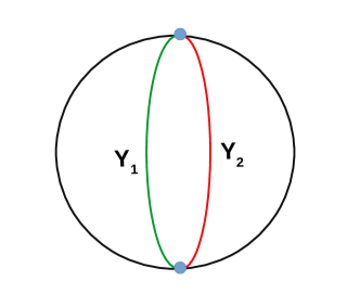
Figure 1: Pictorial representation of wedge holography in a single de-Sitter space. Green and red curves denote EOW branes at $\omega=\omega_{1}$ ($Y_{1}$) and $\omega=\omega_{2}$ ($Y_{2}$). Blue dots are $(d-2)$-dimensional defects.

Wedge holography by joining two copies of double holography in de-Sitter space: Here, we discuss the idea that will play an important role in constructing extended static patch wedge holography. The wedge holography in de-Sitter space can also be described pictorially, as shown in Fig. 2.

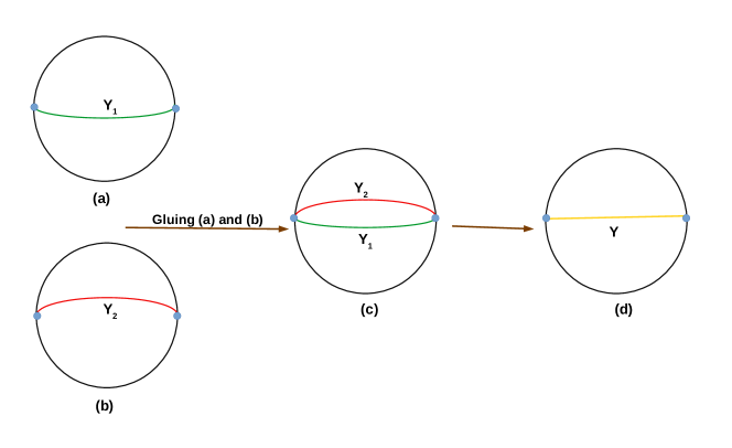
Figure 2: Pictorial representation of wedge holography in de-Sitter space. Green and red curves denote EOW branes at $\omega=\omega_{1}$ ($Y_{1}$) and $\omega=\omega_{2}$ ($Y_{2}$). We can glue (a) and (b) [51] which results in (c) and (d).

We take the spatial slice of de-Sitter space and take a constant $\omega$ slice at $\omega=\omega_{1}$; this is analogous to chopping off the geometry beyond $\omega=\omega_{1}$ (description (a) in Fig. 2). We call this slice as $Y_{1}$. Similarly, we take one more copy of the setup above and chop off the geometry at $\omega=\omega_{2}$; we name this constant $\omega$ slice as $Y_{2}$ (description (b) in Fig. 2). Now we join (a) and (b) using [51]. Conditions for gluing $Y_{1}$ (with metric $\hat{g}_{ij}^{(1)}$, tension $T^{(1)}$) and $Y_{2}$ (with metric $\hat{g}_{ij}^{(2)}$, tension $T^{(2)}$) are Israel junction conditions

$$\hat{g}_{ij}^{(1)}=\hat{g}_{ij}^{(2)};\ \ \ \ [K_{ij}]-[K]\hat{g}_{ij}=-(T^{(1)}+T^{(2)})\hat{g}_{ij},$$

where $[K_{ij}]=K_{ij}^{(1)}+K_{ij}^{(2)}$. In the end, $Y_{1}$ and $Y_{2}$ will merge and result in a new brane, say “$Y$”, and we see that we joined two de-Sitter spaces and obtained a new de-Sitter space.

Therefore, if we compare the above construction of the wedge holography in de-Sitter space with the usual construction in AdS bulk, then we see that we can see a wedge holography-like structure as long as $Y_{1}$ and $Y_{2}$ are separated. Whenever two EOW branes $Y_{1}$ and $Y_{2}$ merge into a single brane $Y$, we obtain a single de-Sitter space instead of wedge holography.

In the next section, we will construct wedge holography for the de-Sitter bulk for the extended static patch, including two Randall-Sundrum branes [53, 54]. In that case, wedge holography is constructed by two Randall-Sundrum branes $Q_{1}$ and $Q_{2}$, similar to the wedge holography in AdS bulk.

3 Wedge holography in extended static patch

Authors in [49] constructed double holography in an extended static patch in the context of DS/dS correspondence. The bulk metric of ($d+1$)-dimensional de-Sitter space is

$$ds_{d+1}^{2}=d\omega^{2}+\sin^{2}(\omega)ds_{d}^{2}=d\omega^{2}+\sin^{2}(\omega)\left(-\cos^{2}\beta dt^{2}+d\beta^{2}+\sin^{2}\beta d\Omega_{d-2}^{2}\right),$$ (30)

where $\beta\in(0,\pi)$ for $d\geq 3$ and $d\Omega_{d-2}^{2}=d\chi^{2}+\sin^{2}\chi d\Omega_{d-3}^{2}$ such that $0\leq\chi\leq\pi$ for $d\geq 4$. The idea to construct double holography is that we need to consider two d-dimensional de-Sitter branes, dS${}_{d}^{1}$ and dS${}_{d}^{2}$ and treat dS${}_{d}^{1}$ brane as Randall-Sundrum brane $Q$ (described by $\chi=\pi/2$) slice and take the $\mathbb{Z}_{2}$ quotient of dS${}_{d}^{2}$, i.e., dS${}_{d}^{2}/\mathbb{Z}_{2}$ which removes half of de-Sitter space of dS${}_{d}^{2}$ and its spatial slice looks like hemisphere. In [49], dS${}_{d}^{2}/\mathbb{Z}_{2}$ is described by $\omega=\pi/2$ slice and is treated as a bath analogous to double holography in AdS backgrounds. In de-Sitter double holography, $d$-dimensional Randall-Sundrum brane $Q$ interact with dS${}_{d}^{2}/\mathbb{Z}_{2}$ via $(d-1)$-dimensional defect where authors considered transparent boundary conditions.

Since $\omega=\pi/2$ slice is the UV part of the geometry [11] therefore, we can treat dS${}_{d}^{2}/\mathbb{Z}_{2}$ as the UV brane. By following [51], we can glue two copies of the double holography described above, and this is described pictorially in Fig. 3.

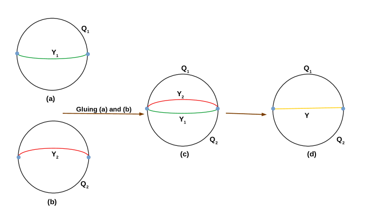
Figure 3: Realization of wedge holography in DS/dS correspondence. Green and red curves denote UV branes $Y_{1}$ and $Y_{2}$ at $\omega_{1,2}=\pi/2$. (a) and (b) are joined along the branes $Y_{1}$ and $Y_{2}$ which results in the final picture (d).

Mathematical descriptions of gluing two copies of double holography are discussed below.

• Consider the bulk metric as

  $$ds_{d+1}^{2}=d\omega_{1}^{2}+\sin^{2}(\omega_{1})dS_{d}^{2}$$

  $$\hskip 28.90755pt=d\omega_{1}^{2}+\sin^{2}(\omega_{1})\left(-\cos^{2}\beta dt^{2}+d\beta^{2}+\sin^{2}\beta\left(d\chi_{1}^{2}+\sin^{2}{\chi_{1}}d\Omega_{d-3}^{2}\right)\right).$$ (31)

  In geometry (• ‣ 3), we consider two slicing, $\omega_{1}=\pi/2$ [dS${}_{d}^{2}/\mathbb{Z}_{2}$, we denote this as $Y_{1}$] and $\chi=\pi/2$ [Randall-Sundrum brane, $Q_{1}$ which is dS${}_{d}^{1}$]. $Q_{1}$ interact with $Y_{1}$ via the transparent boundary conditions at the $(d-1)$-dimensional defect.

• Let us take the bulk metric as

  $$ds_{d+1}^{2}=d\omega_{2}^{2}+\sin^{2}(\omega_{2})dS_{d}^{2}$$

  $$\hskip 28.90755pt=d\omega_{2}^{2}+\sin^{2}(\omega_{2})\left(-\cos^{2}\beta dt^{2}+d\beta^{2}+\sin^{2}\beta\left(d\chi_{2}^{2}+\sin^{2}{\chi_{2}}d\Omega_{d-3}^{2}\right)\right).$$ (32)

  In the bulk (• ‣ 3), $\omega_{2}=\pi/2$ slice is dS${}_{d}^{4}/\mathbb{Z}_{2}$ ($Y_{2}$) and $\chi=\pi/2$ slice is dS${}_{d}^{3}$ (Randall-Sundrum brane, $Q_{2}$). The interaction between $Q_{2}$ and $Y_{2}$ is happening due to the transparent boundary conditions at the $(d-1)$-dimensional defect.

In double holography, the space available is between the Randall-Sundrum brane $Q$ and UV brane $Y$. In this case, wedge holography consists of two $d$-dimensional Randall-Sundram branes $Q_{1}$ and $Q_{2}$, which are joined at the $(d-1)$-dimensional defect. In the language of [51], we have a de-Sitter space bounded between $Q_{1}$ and $Q_{2}$.

Therefore, wedge holography in the extended static patch is constructed by two Randall-Sundrum branes $Q_{1}$ and $Q_{2}$ (description (d) in Fig. 3). We have ($d+1$)-dimensional de-Sitter gravity in the bulk, which is localized on the $d$-dimensional Randall-Sundrum branes $Q_{1}$ and $Q_{2}$. Randall-Sundrum branes $Q_{1}$ and $Q_{2}$ form a wedge, and Randall-Sundrum branes are joined at the ($d-1$)-dimensional defect (blue dots in description (d) of Fig. 3).

4 Communicating universes in extended static patch wedge holography?

The setup described in section 3 can describe the communicating universes similar to [7]. We consider “$n$” copies of the wedge holography discussed in section 3 to describe communicating universes. For three copies, we have Randall-Sundrum branes as $Q_{1,2,3,4,5,6}$ and UV branes as $Y_{1,2,3,4,5,6}$ . Communicating universes are obtained by joining $Y_{1}$ with $Y_{2}$, $Q_{1}$ with $Q_{4}$, $Y_{3}$ with $Y_{4}$, $Q_{3}$ with $Q_{6}$ and so on. This is represented in Fig. 4.

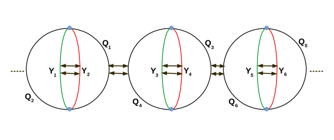
Figure 4: Communicating universes in de-Sitter wedge holography.

If we follow the above idea and join the various branes following [51], then Fig. 4 end up at the end of gluing as shown in Fig. 5 where we have replaced “sphere” with “box” only for convenience so that we can draw the cartoon picture easily. The notations are, e.g., $Q_{14}=Q_{1}+Q_{4}$, $Y_{12}=Y_{1}+Y_{2}$, $Q_{36}=Q_{3}+Q_{6}$, $Y_{34}=Y_{3}+Y_{4}$ and so on; in general $Q_{ij}=Q_{i}+Q_{j}$ and $Y_{ij}=Y_{i}+Y_{j}$ where $i$ and $j$ are the labels of the branes.

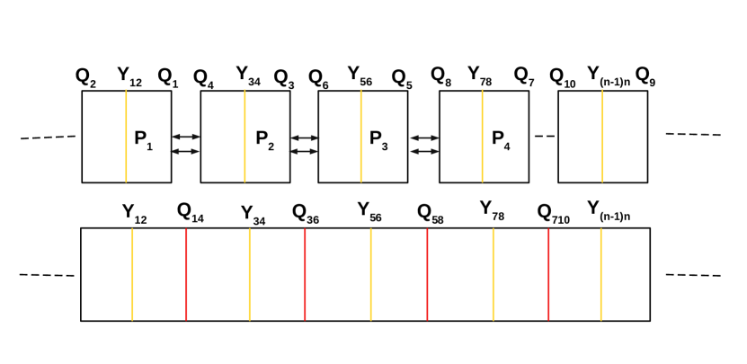
Figure 5: Structure of the communicating universes in de-Sitter wedge holography. We have represented the gluing of $Y_{i}$’s brane ($Y_{ij}=Y_{i}+Y_{j}$) in yellow color whereas the gluing of Randall-Sundrum branes, $Q_{i}$’s ($Q_{ij}=Q_{i}+Q_{j}$) by red color.

Let us understand the physical meaning of Fig. 4 and 5. In the beginning, we take two copies of double holography in DS/dS correspondence [49], and we obtain the geometrical structure as the one copy of wedge holography as shown in Fig. 4 with Randall-Sundrum branes $Q_{1,2}$ and UV branes $Y_{1,2}$. When we join $Y_{1}$ and $Y_{2}$ using [51], then we obtain the first box as shown in the upper part of Fig. 5 with Randall-Sundrum branes $Q_{1}$ and $Q_{2}$ and one UV brane $Y_{12}$. This describes a single de-Sitter space with cut-off by the Randall-Sundrum branes $Q_{1}$ and $Q_{2}$. We can treat this kind of box as a building block (say $P_{1}$) and then join many copies of this building block as shown in the upper part of Fig. 5, e.g., $P_{1}$ with $P_{2}$, $P_{2}$ with $P_{3}$, $P_{3}$ with $P_{4}$ and so on. $P_{i}$’s are like a single de-Sitter space with two Randall-Sundrum branes. As long as $P_{i}$s are separated, this model will provide the structure of parallel universes. Whenever we join all the $P_{i}$’s with each other, then we obtain the lower part of Fig. 5, which describes a single de-Sitter space with two Randall-Sundrum branes at the end of de-Sitter space. Hence, the existence of a parallel universe in extended static patch holography depends upon whether we join all copies of extended static patch holography or not.

5 Communicating Multiverses in de-Sitter wedge holography

This section discusses the existence of multiverse and communicating multiverses in de-Sitter wedge holography via subsections 5.1 and 5.2.

5.1 Multiverse

We can construct a multiverse for a single de-Sitter space as shown in Fig. 6.

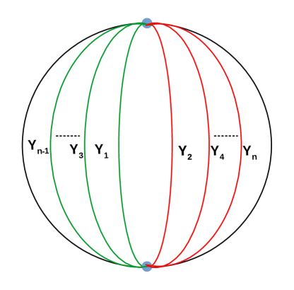
Figure 6: Multiverse in de-Sitter wedge holography. $Y_{1,2,...,n-1,n}$ are the constant $\omega$ slices in a single de-Sitter space.

We obtain the Multiverse model in a single de-Sitter space by taking the constant $\omega$ slices of a single de-Sitter bulk (2.1). As we discussed earlier, we have Einstein gravity with positive cosmological constant on constant $\omega$ slices, and hence we have a Multiverse made up of “$n$” universes with geometry on each of them as dS_d-1, and all these universes are embedded in a single de-Sitter bulk with geometry dS_d. This kind of model for the AdS bulk was discussed in [6]. Here, we are able to construct the Multiverse model in de-Sitter space which is more realistic as we are living in a universe with positive cosmological constant. One can check that the bulk metric (2.1) satisfies the Neumann boundary condition (7) at $\omega=\omega_{1,2,....,n-1,n}$ provided tensions of the end-of-the-world branes should be given as follows

$$T^{\beta}=\frac{d-2}{R}\cot\left(\frac{\omega_{1,2,....,n-1,n}}{R}\right),$$ (33)

where $\beta=1,2,....,n-1,n$. The interesting point about this setup is that all the universes ($Y_{1}$, $Y_{2}$,….,$Y_{n-1}$, and $Y_{n}$) are joined at the single defect (blue dot in Fig. 6) and hence there is the possibility of exchange of information among each other.

5.2 Communicating Multiverses

Given that Multiverse exists in de-Sitter wedge holography as discussed in subsection 5.1. Now, we discuss the possibility of the existence of communicating multiverses. It is possible by joining many copies of the Multiverse as shown in Fig. 7.

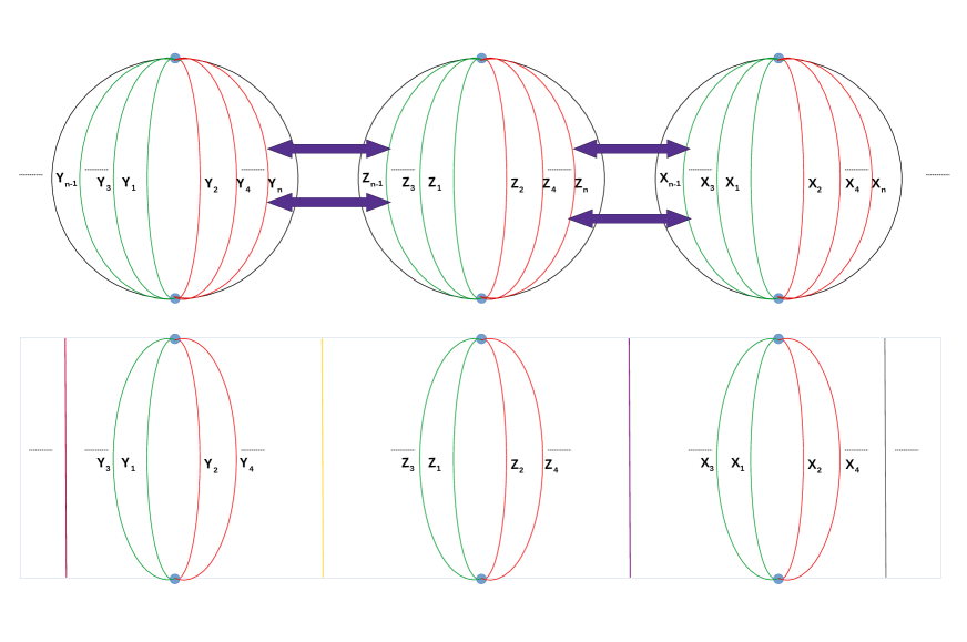
Figure 7: Communicating multiverses in de-Sitter wedge holography. For simplicity, we replaced the sphere with a rectangle in the lower part of this figure.

To do so, we join $n$th brane of one copy with $(n-1)$th brane of the second copy, $n$th brane of the second copy with $(n-1)$th brane of the third copy, and so on; this is represented pictorially in Fig. 7. More precisely, the left outermost brane of the first copy will join with the right outermost brane of the second copy; the left outermost brane of the second copy will join with the rightmost outer brane of the third copy, and so on. We have done it for three copies in Fig. 7.

In the process of constructing communicating multiverses, we have to lose some of the universes. For example, if we join two multiverses, then we have to lose two universes: one from the left copy($Y_{n}$) and one copy from the other copy ($Z_{n-1}$). These two branes will form a new brane, which is represented by a yellow line in the lower part of Fig. 7. Similarly, if we join Multiverse made up of $Z_{1,2,...,n-1,n}$-branes with the Multiverse made up of $X_{1,2,....,n-1,n}$ branes, then the combination of $Z_{n}$ brane and $X_{n-1}$ brane will form a new brane and the same is represented by dark purple in the lower part of Fig. 7.

To have a consistent model of communicating multiverses, we have to stop the process of joining branes from the consecutive multiverses; otherwise, all left branes of one copy will join with the all right branes of the right copy, and at the end, we have a single universe as obtained in section 4. To be more specific in the context of Fig. 7, all the left branes of multiverse “$Y$”(which consist of universes $Y_{1,2,...,n-1,n}$) will join with all the right branes of multiverse “$Z$” consists of universes $Z_{1,2,...,n-1,n}$; all the left branes of multiverse “$Z$” with universes $Z_{1,2,...,n-1,n}$ will join with all the right branes of multiverse “$X$” with universes $X_{1,2,...,n-1,n}$ and so on. In the end, we obtain a single de-Sitter space cut-off by two end-of-the-world branes.

6 Discussion

In this paper, we have constructed the wedge holography for the de-Sitter space and discussed its application to multiverse models. First, we did this for general de-Sitter background using the idea similar to AdS bulk in section 2 where we used the localization of de-Sitter gravity [50] on the brane. A clue to the dS_d/CFT_d-2 duality is provided by this. In this case, it is possible to obtain a multiverse-like structure by taking many constant $\omega$ slices of single de-Sitter space, see Fig. 6. We see the existence of communicating multiverses [Fig. 7] by gluing many multiverses with each other following the concept of [51]. It must be noted that communicating multiverses exist as long as all left branes of one multiverse are not joined with the all right branes of the other multiverse. Otherwise, we obtain a single de-Sitter space bounded by two end-of-the-world branes.

In section 3, we constructed wedge holography in the extended static patch. This was done using the idea of double holography in DS/dS correspondence [49]. We can construct wedge holography in this case by gluing two copies of a doubly holographic setup by following [51]. We can have four branes in extended static patch wedge holography if we keep separating the UV branes $Y_{1}$ and $Y_{2}$. If we join them, we obtain wedge holography with two Randall-Sundrum branes $Q_{1}$ and $Q_{2}$, see Fig. 3. It is nice to see that one can describe parallel universes from the perspective of wedge holography. This can be achieved by taking “$n$” copies of wedge holography and then gluing them together in parallel. Again, parallel universes exist as long as “$n$” copies are not completely joined, i.e., we can have disconnected parallel universes. If we join the left brane of one copy with the right brane of the other, we obtain a single de-Sitter space bounded by two Randall-Sundrum branes (Fig. 5).

Based on the theoretical construction of Multiverse discussed in subsection 5.1, we can say that we are living in a universe that is part of the Multiverse because this model is constructed in de-Sitter space, which has a positive cosmological constant. Many universes exist (where different species may be living) within the same Multiverse, but we are not able to travel among other universes because of our limitations. Suppose we are living in a universe and we want to travel in a different universe, then we have to cross the defect that is common to both universes. In this paper, we have not discussed this issue, but we hope to explore it in our future work. We have made a qualitative statement on this issue in [6] for the AdS bulk spacetime.

In subsection 5.2, in the process of constructing communicating multiverses. There is a possibility that we can have disconnected multiverses. In this scenario, there can’t be any communication between any universe of one Multiverse and any universe of another multiverse. However, to make the communication between two multiverses, we need to have connected multiverses where one universe (left outermost) of one Multiverse will get combined with one universe(right outermost) of the other Multiverse. In this case, there could be possibility of communication between different multiverses.

It would be interesting if one could construct this kind of model from top-down holography similar to [55] where the authors discussed the existence of binary black holes from top-down triple holography. So far we have discussed the existence of parallel universes, multiverses, and communicating multiverses for the identical branes, i.e., we have multiple copies of the same universe. As we discussed in [6] that issue of mismatched branes [60] was present even in wedge holography which prevented us to contruct the wedge holographic realization of Schwarzschild de-Sitter black hole. If one could resolve the issue of mismatched branes from the perspective of [51] then one may obtain the Page curve of Schwarzschild de-Sitter black hole [62, 61, 63] from wedge holography. It would be nice to include the grey-body factors [64] and see the affect of the same on information exchange between different universes or in usual wedge holography where Hawking radiation is exchanged between gravitating branes. Further, one can use our model to discuss the information paradox in de-Sitter space by considering one brane as the source of Gibbons-Hawking radiation [65] and another as a bath for collecting the Gibbons-Hawking radiation.

References

- [1] M. Tegmark, Parallel universes, Science and Ultimate Reality: From Quantum to Cosmos, honoring John Wheeler’s 90th birthday. J. D. Barrow, P.C.W. Davies, and C.L. Harper eds. Cambridge University Press [arXiv:astro-ph/0302131 [astro-ph]].
- [2] M. Kaku, PARALLEL WORLDS: A Journey Through Creation, Higher Dimensions, and the Future of the Cosmos.
- [3] R. Bousso and L. Susskind, “The Multiverse Interpretation of Quantum Mechanics,” Phys. Rev. D 85, 045007 (2012) doi:10.1103/PhysRevD.85.045007 [arXiv:1105.3796 [hep-th]].
- [4] Y. Nomura, “The Static Quantum Multiverse,” Phys. Rev. D 86, 083505 (2012) doi:10.1103/PhysRevD.86.083505 [arXiv:1205.5550 [hep-th]].
- [5] A. Linde, “A brief history of the multiverse,” Rept. Prog. Phys. 80, no.2, 022001 (2017) doi:10.1088/1361-6633/aa50e4 [arXiv:1512.01203 [hep-th]].
- [6] G. Yadav, “Multiverse in Karch-Randall Braneworld,” JHEP 03, 103 (2023) doi:10.1007/JHEP03(2023)103 [arXiv:2301.06151 [hep-th]].
- [7] S. E. Aguilar-Gutierrez and F. Landgren, “A multiverse model in dS wedge holography,” [arXiv:2311.02074 [hep-th]].
- [8] J. M. Maldacena, “The Large N limit of superconformal field theories and supergravity,” Adv. Theor. Math. Phys. 2, 231-252 (1998) doi:10.4310/ATMP.1998.v2.n2.a1 [arXiv:hep-th/9711200 [hep-th]].
- [9] A. Strominger, “The dS/CFT correspondence,” JHEP 10, 034 (2001) doi:10.1088/1126-6708/2001/10/034 [arXiv:hep-th/0106113 [hep-th]].
- [10] J. M. Maldacena, “Non-Gaussian features of primordial fluctuations in single field inflationary models,” JHEP 05, 013 (2003) doi:10.1088/1126-6708/2003/05/013 [arXiv:astro-ph/0210603 [astro-ph]].
- [11] M. Alishahiha, A. Karch, E. Silverstein and D. Tong, “The dS/dS correspondence,” AIP Conf. Proc. 743, no.1, 393-409 (2004) doi:10.1063/1.1848341 [arXiv:hep-th/0407125 [hep-th]].
- [12] M. Mia, K. Dasgupta, C. Gale and S. Jeon, “Five Easy Pieces: The Dynamics of Quarks in Strongly Coupled Plasmas,” Nucl. Phys. B 839, 187-293 (2010) doi:10.1016/j.nuclphysb.2010.06.014 [arXiv:0902.1540 [hep-th]].
- [13] M. Dhuria and A. Misra, “Towards MQGP,” JHEP 11, 001 (2013) doi:10.1007/JHEP11(2013)001 [arXiv:1306.4339 [hep-th]].
- [14] A. Misra and V. Yadav, “On -Theory Dual of Large- Thermal QCD-Like Theories up to and -Structure Classification of Underlying Non-Supersymmetric Geometries,” Adv. Theor. Math. Phys. 26, 10 (2022) [arXiv:2004.07259 [hep-th]].
- [15] S. A. Hartnoll, C. P. Herzog and G. T. Horowitz, “Building a Holographic Superconductor,” Phys. Rev. Lett. 101, 031601 (2008) doi:10.1103/PhysRevLett.101.031601 [arXiv:0803.3295 [hep-th]].
- [16] S. Ryu and T. Takayanagi, “Topological Insulators and Superconductors from D-branes,” Phys. Lett. B 693, 175-179 (2010) doi:10.1016/j.physletb.2010.08.019 [arXiv:1001.0763 [hep-th]].
- [17] S. R. Das, J. Michelson, K. Narayan and S. P. Trivedi, “Time dependent cosmologies and their duals,” Phys. Rev. D 74, 026002 (2006) doi:10.1103/PhysRevD.74.026002 [arXiv:hep-th/0602107 [hep-th]].
- [18] A. Awad, S. R. Das, K. Narayan and S. P. Trivedi, “Gauge theory duals of cosmological backgrounds and their energy momentum tensors,” Phys. Rev. D 77, 046008 (2008) doi:10.1103/PhysRevD.77.046008 [arXiv:0711.2994 [hep-th]].
- [19] A. Awad, S. R. Das, S. Nampuri, K. Narayan and S. P. Trivedi, “Gauge Theories with Time Dependent Couplings and their Cosmological Duals,” Phys. Rev. D 79, 046004 (2009) doi:10.1103/PhysRevD.79.046004 [arXiv:0807.1517 [hep-th]].
- [20] V. Balasubramanian, P. Hayden, A. Maloney, D. Marolf and S. F. Ross, “Multiboundary Wormholes and Holographic Entanglement,” Class. Quant. Grav. 31, 185015 (2014) doi:10.1088/0264-9381/31/18/185015 [arXiv:1406.2663 [hep-th]].
- [21] A. Al Balushi, Z. Wang and D. Marolf, “Traversability of Multi-Boundary Wormholes,” JHEP 04, 083 (2021) doi:10.1007/JHEP04(2021)083 [arXiv:2012.04635 [hep-th]].
- [22] K. Jalan and R. Pius, “Half-sided Translations and Islands,” [arXiv:2312.11085 [hep-th]].
- [23] G. Araujo-Regado, R. Khan and A. C. Wall, “Cauchy slice holography: a new AdS/CFT dictionary,” JHEP 03, 026 (2023) doi:10.1007/JHEP03(2023)026 [arXiv:2204.00591 [hep-th]].
- [24] S. W. Hawking, “Particle Creation by Black Holes,” Commun. Math. Phys. 43, 199-220 (1975) [erratum: Commun. Math. Phys. 46, 206 (1976)] doi:10.1007/BF02345020.
- [25] A. Almheiri, R. Mahajan, J. Maldacena and Y. Zhao, “The Page curve of Hawking radiation from semiclassical geometry,” JHEP 03, 149 (2020) doi:10.1007/JHEP03(2020)149 [arXiv:1908.10996 [hep-th]].
- [26] A. Almheiri, T. Hartman, J. Maldacena, E. Shaghoulian and A. Tajdini, “The entropy of Hawking radiation,” Rev. Mod. Phys. 93, no.3, 035002 (2021) doi:10.1103/RevModPhys.93.035002 [arXiv:2006.06872 [hep-th]].
- [27] A. Almheiri, R. Mahajan and J. E. Santos, “Entanglement islands in higher dimensions,” SciPost Phys. 9, no.1, 001 (2020) doi:10.21468/SciPostPhys.9.1.001 [arXiv:1911.09666 [hep-th]].
- [28] T. Takayanagi, “Holographic Dual of BCFT,” Phys. Rev. Lett. 107, 101602 (2011) doi:10.1103/PhysRevLett.107.101602 [arXiv:1105.5165 [hep-th]].
- [29] M. Fujita, T. Takayanagi and E. Tonni, “Aspects of AdS/BCFT,” JHEP 11, 043 (2011) doi:10.1007/JHEP11(2011)043 [arXiv:1108.5152 [hep-th]].
- [30] I. Akal, Y. Kusuki, T. Takayanagi and Z. Wei, “Codimension two holography for wedges,” Phys. Rev. D 102, no.12, 126007 (2020) doi:10.1103/PhysRevD.102.126007 [arXiv:2007.06800 [hep-th]].
- [31] R. X. Miao, “An Exact Construction of Codimension two Holography,” JHEP 01, 150 (2021) doi:10.1007/JHEP01(2021)150 [arXiv:2009.06263 [hep-th]].
- [32] D. N. Page, “Information in black hole radiation,” Phys. Rev. Lett. 71, 3743-3746 (1993) doi:10.1103/PhysRevLett.71.3743 [arXiv:hep-th/9306083 [hep-th]].
- [33] T. Hartman and J. Maldacena, “Time Evolution of Entanglement Entropy from Black Hole Interiors,” JHEP 05, 014 (2013) doi:10.1007/JHEP05(2013)014 [arXiv:1303.1080 [hep-th]].
- [34] A. Karch and L. Randall, “Locally localized gravity,” JHEP 05, 008 (2001) doi:10.1088/1126-6708/2001/05/008 [arXiv:hep-th/0011156 [hep-th]].
- [35] A. Karch and L. Randall, “Open and closed string interpretation of SUSY CFT’s on branes with boundaries,” JHEP 06, 063 (2001) doi:10.1088/1126-6708/2001/06/063 [arXiv:hep-th/0105132 [hep-th]].
- [36] H. Geng, A. Karch, C. Perez-Pardavila, S. Raju, L. Randall, M. Riojas and S. Shashi, “Information Transfer with a Gravitating Bath,” SciPost Phys. 10, no.5, 103 (2021) doi:10.21468/SciPostPhys.10.5.103 [arXiv:2012.04671 [hep-th]].
- [37] P. J. Hu and R. X. Miao, “Effective action, spectrum and first law of wedge holography,” JHEP 03, 145 (2022) doi:10.1007/JHEP03(2022)145 [arXiv:2201.02014 [hep-th]].
- [38] H. Geng, A. Karch, C. Perez-Pardavila, S. Raju, L. Randall, M. Riojas and S. Shashi, “Jackiw-Teitelboim Gravity from the Karch-Randall Braneworld,” Phys. Rev. Lett. 129, no.23, 231601 (2022) doi:10.1103/PhysRevLett.129.231601 [arXiv:2206.04695 [hep-th]].
- [39] H. Geng, “Aspects of AdS2 quantum gravity and the Karch-Randall braneworld,” JHEP 09, 024 (2022) doi:10.1007/JHEP09(2022)024 [arXiv:2206.11277 [hep-th]].
- [40] R. X. Miao, “Massless Entanglement Island in Wedge Holography,” [arXiv:2212.07645 [hep-th]].
- [41] R. X. Miao, “Entanglement island and Page curve in wedge holography,” JHEP 03, 214 (2023) doi:10.1007/JHEP03(2023)214 [arXiv:2301.06285 [hep-th]].
- [42] D. Li and R. X. Miao, “Massless entanglement islands in cone holography,” JHEP 06, 056 (2023) doi:10.1007/JHEP06(2023)056 [arXiv:2303.10958 [hep-th]].
- [43] A. Bhattacharya, A. Bhattacharyya and A. K. Patra, “Holographic complexity of Jackiw-Teitelboim gravity from Karch-Randall braneworld,” JHEP 07, 060 (2023) doi:10.1007/JHEP07(2023)060 [arXiv:2304.09909 [hep-th]].
- [44] H. Geng, A. Karch, C. Perez-Pardavila, L. Randall, M. Riojas, S. Shashi and M. Youssef, “Constraining braneworlds with entanglement entropy,” SciPost Phys. 15, no.5, 199 (2023) doi:10.21468/SciPostPhys.15.5.199 [arXiv:2306.15672 [hep-th]].
- [45] R. X. Miao, “Ghost Problem, Spectrum Identities and Various Constraints on Brane-localized Higher Derivative Gravity,” [arXiv:2310.16297 [hep-th]].
- [46] Z. Q. Cui, Y. Guo and R. X. Miao, “Cone Holography with Neumann Boundary Conditions and Brane-localized Gauge Fields,” [arXiv:2312.16463 [hep-th]].
- [47] R. X. Miao, “Entanglement island versus massless gravity,” Eur. Phys. J. C 84, no.2, 123 (2024).
- [48] N. Ogawa, T. Takayanagi, T. Tsuda and T. Waki, “Wedge holography in flat space and celestial holography,” Phys. Rev. D 107, no.2, 026001 (2023) doi:10.1103/PhysRevD.107.026001 [arXiv:2207.06735 [hep-th]].
- [49] H. Geng, Y. Nomura and H. Y. Sun, “Information paradox and its resolution in de Sitter holography,” Phys. Rev. D 103, no.12, 126004 (2021) doi:10.1103/PhysRevD.103.126004 [arXiv:2103.07477 [hep-th]].
- [50] A. Karch, “Autolocalization in de Sitter space,” JHEP 07, 050 (2003) doi:10.1088/1126-6708/2003/07/050 [arXiv:hep-th/0305192 [hep-th]].
- [51] T. Kawamoto, S. M. Ruan and T. Takayanagia, “Gluing AdS/CFT,” JHEP 07, 080 (2023) doi:10.1007/JHEP07(2023)080 [arXiv:2303.01247 [hep-th]].
- [52] G. Yadav and H. Rathi, “Yang-Baxter deformed wedge holography,” Phys. Lett. B 852, 138592 (2024) doi:10.1016/j.physletb.2024.138592 [arXiv:2307.01263 [hep-th]].
- [53] L. Randall and R. Sundrum, “An Alternative to compactification,” Phys. Rev. Lett. 83, 4690-4693 (1999) doi:10.1103/PhysRevLett.83.4690 [arXiv:hep-th/9906064 [hep-th]].
- [54] L. Randall and R. Sundrum, “A Large mass hierarchy from a small extra dimension,” Phys. Rev. Lett. 83, 3370-3373 (1999) doi:10.1103/PhysRevLett.83.3370 [arXiv:hep-ph/9905221 [hep-ph]].
- [55] E. Deddo, L. A. Pando Zayas and C. F. Uhlemann, “Binary AdS black holes coupled to a bath in Type IIB,” [arXiv:2401.00511 [hep-th]].
- [56] C. F. Uhlemann, “Islands and Page curves in 4d from Type IIB,” JHEP 08, 104 (2021) doi:10.1007/JHEP08(2021)104 [arXiv:2105.00008 [hep-th]].
- [57] A. Karch, H. Sun and C. F. Uhlemann, “Double holography in string theory,” JHEP 10, 012 (2022) doi:10.1007/JHEP10(2022)012 [arXiv:2206.11292 [hep-th]].
- [58] G. Yadav and A. Misra, “Entanglement entropy and Page curve from the M-theory dual of thermal QCD above Tc at intermediate coupling,” Phys. Rev. D 107, no.10, 106015 (2023) doi:10.1103/PhysRevD.107.106015 [arXiv:2207.04048 [hep-th]].
- [59] H. Bernardo, S. Brahma, K. Dasgupta and R. Tatar, “Crisis on Infinite Earths: Short-lived de Sitter Vacua in the String Theory Landscape,” JHEP 04, 037 (2021) doi:10.1007/JHEP04(2021)037 [arXiv:2009.04504 [hep-th]].
- [60] A. Karch and L. Randall, “Geometries with mismatched branes,” JHEP 09, 166 (2020) doi:10.1007/JHEP09(2020)166 [arXiv:2006.10061 [hep-th]].
- [61] K. Goswami and K. Narayan, “Small Schwarzschild de Sitter black holes, quantum extremal surfaces and islands,” JHEP 10, 031 (2022) doi:10.1007/JHEP10(2022)031 [arXiv:2207.10724 [hep-th]].
- [62] G. Yadav and N. Joshi, “Cosmological and black hole islands in multi-event horizon spacetimes,” Phys. Rev. D 107, no.2, 026009 (2023) doi:10.1103/PhysRevD.107.026009 [arXiv:2210.00331 [hep-th]].
- [63] K. Goswami and K. Narayan, “Small Schwarzschild de Sitter black holes, the future boundary and islands,” [arXiv:2312.05904 [hep-th]].
- [64] T. J. Hollowood, S. P. Kumar, A. Legramandi and N. Talwar, “Grey-body factors, irreversibility and multiple island saddles,” JHEP 03, 110 (2022) doi:10.1007/JHEP03(2022)110 [arXiv:2111.02248 [hep-th]].
- [65] G. W. Gibbons and S. W. Hawking, “Cosmological Event Horizons, Thermodynamics, and Particle Creation,” Phys. Rev. D 15, 2738-2751 (1977) doi:10.1103/PhysRevD.15.2738.