Generalized Maximum Entropy Differential Dynamic Programming

Abstract

We present a sampling-based trajectory optimization method derived from the maximum entropy formulation of Differential Dynamic Programming with Tsallis entropy. This method can be seen as a generalization of the legacy work with Shannon entropy, which leads to a Gaussian optimal control policy for exploration during optimization. With the Tsallis entropy, the optimal control policy takes the form of $q$-Gaussian, which further encourages exploration with its heavy-tailed shape. Moreover, in our formulation, the exploration variance, which was scaled by a fixed constant inverse temperature in the original formulation with Shannon entropy, is automatically scaled based on the value function of the trajectory. Due to this property, our algorithms can promote exploration when necessary, that is, the cost of the trajectory is high, rather than using the same scaling factor. The simulation results demonstrate the properties of the proposed algorithm described above.

I Introduction

Tsallis entropy, also known as $q$-logarithmic entropy is a generalization of standard Boltzmann-Gibbs or Shannon entropy [1, 2]. The Tsallis entropy is nonadditive, which means that the sum of the entropy of probabilistically independent subsystems is not equal to that of the entire system. The entropy is used in nonextensive statistical mechanics which can handle strongly correlated random variables[3, 4]. It helps to analyze complex phenomena in physics such as in [5, 6], etc.

Maximization of Shannon entropy under fixed mean and covariance yields a Gaussian distribution [7]. With the Tsallis entropy, similar maximization with a fixed $q$-mean and covariance leads to a $q$-Gaussian distribution [8, 9]. With a certain range of the entropic index $q$, the distribution has a heavy tail compared to a normal Gaussian. Due to this property, the $q$-Gaussian distribution is utilized for several engineering applications. In [10] a mixture of the distribution is used for image and video semantic mapping, improving the robustness to outliers. In stochastic optimization, the distribution is used as a generalization of the Gaussian kernel, achieving better control over the smoothing of functions compared to the normal Gaussian [11]. It was also used for mutation in the evolutionary algorithm, showing its effectiveness over the Gaussian and Cauchy distributions [12].

Maximum entropy is a popular technique in various fields, such as Stochastic Optimal Control (SOC) and Reinforcement Learning (RL), which can improve the robustness of stochastic policies. Robustness is achieved by adding an entropic regularization term to the objective, which prevents the policies from converging to a delta distribution by encouraging exploration during optimization while simultaneously maximizing entropy [13, 14]. In SOC, Shannon entropy, which leads to Kullback-Leibler (KL) divergence, is used as a regularization term between the controlled and prior distributions [15]. In [16], Tsallis divergence, a generalization of the KL divergence, is used, showing improvements in robustness. For RL application, Tsallis entropic regularization leads to better performance and faster convergence [17, 18, 19]. Recently, the technique with Shannon entropy has been applied to a trajectory optimization algorithm Differential Dynamic Programming (DDP) [20], which yields the Maximum Entropy DDP (ME-DDP)[21]. DDP is a powerful trajectory optimization tool that has a quadratic convergence rate [22]. However, since it relies on local information, of cost and dynamics, it converges to local minima rather than global minima. ME-DDP can explore multiple local minima while minimizing the original objective. Consequently, it can find better local minima than those of normal DDP without exploration.

In this paper, we propose ME-DDP with Tsallis entropy, which is a generalization of ME-DDP with Shannon entropy. The Tsallis entropy turns the optimal policy from Gaussian to heavy-tailed $q$-Gaussian, improving the exploration capacity of ME-DDP. Moreover, the generalized formulation can automatically scale the variance of the policy based on the value function (and thus the cost) of the trajectory, which further promotes exploration. We validate our proposed algorithm in two robotic systems, i.e., a 2D car and a quadrotor, and make comparison with normal DDP and ME-DDP with Shannon entropy.

The main contribution of this paper is as follows.

• We derive DDP with Tsallis entropic regularization.

• We show the superior exploration capability of ME-DDP with Tsallis entropy to ME-DDP Shannon entropy by analyzing the stochastic policies.

• We validate the exploration capability of our method with two robotic systems in simulation.

II Preliminaries

II-A Tsallis Entropy

With an entropic index $q\in\mathbb{R}$, we introduce $q$-logarithm function

$$\ln_{q}(x)=\begin{cases}\ln(x),\quad\quad\quad&q=1,\ x>0\\ \frac{x^{1-q}-1}{1-q},\quad&q\neq 1\ x>0,\end{cases}$$ (1)

and its inverse $q$-exponential function

$$\exp_{q}(x)=\begin{cases}\exp(x),\hskip 85.35826pt&q=1,\\ [1-(q-1)x]_{+}^{-\frac{1}{q-1}},&q\neq 1.\end{cases}$$

Consider a discrete set of probabilities $\{p_{i}\}$. $i=1,\cdots,I$. The Tsallis or $q$-entropy is defined as

$$S_{q}(p)=\frac{1-\sum_{i}p_{i}^{q}}{q-1},$$ (2)

which is a generalization of the Shannon entropy

$$H(p)=\sum_{i}p_{i}\log\Big{(}\frac{1}{p_{i}}\Big{)}=-\sum_{i}p_{i}\log{p_{i}}.$$

The Tsallis entropy may be represented as a sum of the product of probability and $q$-$\log$ probability as

$$S_{q}(p) =\sum_{i}p_{i}\ln_{q}\Big{(}\frac{1}{p_{i}}\Big{)}=\sum_{i}p_{i}\frac{p_{i}^{q-1}-1}{1-q}=\frac{1-\sum_{i}p_{i}^{q}}{q-1},$$

which recovers the definition in (2). We believe that this is the most straightforward generalization. Although

$$S_{q}(p)=-\sum_{i}p_{i}\ln_{q}p_{i}$$

can be another option for the definition, the following relation

$$-\ln_{q}p_{i}\neq\ln_{q}(1/p_{i}),$$

changes the parametrization $q$ to $2-q$ as in [18]. Thus, we use the former definition in (2) to avoid this change. The argument above holds with continuous probability distribution by changing summation to integral.

II-B Univariate q-Gaussian distribution

Let us consider a Probability Distribution Function (PDF) $p_{q}(x)$ of a random variable $x\in\mathbb{R}$. $q$-Gaussian distribution is a generalized version of Gaussian distribution, which is obtained by maximizing the $q$-entropy with a fixed (given) $q$-mean $\mu_{q}$ and $q$-variance $\sigma^{2}_{q}$, where subscripts $q$ mean that they are computed with the $q$-escort distribution, which is a $q$ th power of the original $p_{q}(x)$, and normalized by it, i.e.,

$$\mu_{q}=\frac{\int xp_{q}(x)^{q}\mathrm{d}x}{\int p_{q}(x)^{q}\mathrm{d}x},\quad\sigma_{q}^{2}=\frac{\int(x-\mu_{q})^{2}p_{q}(x)^{q}\mathrm{d}x}{\int p_{q}(x)^{q}\mathrm{d}x}.$$

This normalization is known to be the correct formulation of nonextensive statistics[9]. The univariate $q$-Gaussian distribution is given as follows [9].

$$p_{q}(x) =\frac{1}{Z_{q}}\Big{(}1-\frac{1-q}{3-q}\frac{(x-\mu_{q})^{2}}{\sigma_{q}^{2}}\Big{)}^{\frac{1}{1-q}},$$

$$\text{with}\ Z_{q} =\begin{cases}\Big{[}\sigma_{q}^{2}\frac{3-q}{q-1}\Big{]}^{\frac{1}{2}}B\Big{(}\frac{1}{2},\frac{3-q}{2(q-1)}\Big{)},\ 1<q<3,\\ \Big{[}\sigma_{q}^{2}\frac{3-q}{1-q}\Big{]}^{\frac{1}{2}}B\Big{(}\frac{1}{2},\frac{2-q}{1-q}\Big{)},\ q<1,\end{cases}$$

where $B(\cdot,\cdot)$ is Beta function. The bounds for $q$ are for the convergence of integrals to compute the partition function. Here, we provide two properties of the function.
Compact support when $q<1$.
To satisfy $p_{q}(x)\geq 0$, $p_{q}(x)$ has a compact support in the case of $q<1$, which is given by $x\in[x_{b},x_{u}]$, with

$$x_{b}=\mu-a_{q},\ x_{u}=\mu+a_{q},\ a_{q}=\sqrt{{(3-q)}/{(1-q)}}.$$

Note that $\mu_{q}=\mu$ when $q<2$.
Recovers Normal Gaussian as $q\rightarrow 1$.
Using the definition of exponential

$$e^{x}=\lim_{n\rightarrow 0}(1+x/n)^{n},$$

$p_{q}$ approaches

$$p_{1}(x)=\frac{1}{\sqrt{2\pi}\sigma}\exp\Big{[}{-\frac{(x-\mu)^{2}}{2\sigma^{2}}}\Big{]},$$

as $q\rightarrow 1$, which is normal Gaussian distribution.

In addition to these, moments (not $q$-moments, but normal ones) are only defined with certain $q$s due to the convergence condition of integrals. A sampling method from the distribution is proposed in [23].

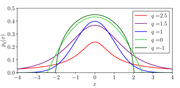
Figure 1: $q$-Gaussian distribution with different $q$s with $\mu_{q}=0$ and $\sigma_{q}^{2}=1$. $q=1$ corresponds to a normal Gaussian.

We show some $p_{q}(x)$ with different $q$ in Fig. 1. As can be seen from the figure, a large $q$ with $q>1$ yields a heavier-tailed distribution than the normal Gaussian ($q=1$). We can also observe the compact support when $q<1$. For exploration purposes, we prefer the heavy-tailed distribution and thus focus on the case where $q>1$, hereafter.

II-C Multivariate q-Gaussian Distribution

The multivariate variant for $q>1$ and $x\in\mathbb{R}^{n}$ is given by

$$p_{q}(x)=\frac{1}{Z_{q}}\Big{[}1+\frac{q-1}{n+2-nq}(x-\mu_{q})^{\mathsf{T}}\Sigma_{q}^{-1}(x-\mu_{q})]^{-\frac{1}{q-1}},$$

$$\text{with}\ Z_{q}=\Big{[}\frac{(n+2)-nq}{q-1}\Big{]}^{\frac{n}{2}}|\Sigma_{q}|^{\frac{1}{2}}\pi^{\frac{n}{2}}\frac{\Gamma\Big{(}\frac{1}{q-1}-\frac{n}{2}\Big{)}}{\Gamma\Big{(}\frac{1}{q-1}\Big{)}},$$ (3)

where $\Gamma(\cdot)$ is Gamma function [24, 25]. Since the argument for the Gamma function needs to be positive, $q$ needs to satisfy the following condition.

$$1<q<1+{2}/{n}.$$ (4)

The $q$-second moment $\Sigma_{q}\in\mathbb{R}^{n\times n}$ and (normal) covariance $\Sigma$ have the following relation.

$$\Sigma=\frac{n+2-nq}{n+4-(n+2)q}\Sigma_{q},$$

whose numerator is positive due to (4). For, $\Sigma>0$, we need

$$1<q<\frac{n+4}{n+2}=1+\frac{2}{n+2},$$

which is always satisfied by as long as (4) is satisfied. Note that (II-C) is equivalent to the Student’s $t$ distribution[26, 7] given by

$$p_{t}(x)$$

$$= \frac{\Gamma(\nu+n)/2}{\Gamma(\nu/2)\nu^{n/2}\pi^{n/2}|\Sigma|}\Big{[}1+\frac{1}{\nu}(x-\mu)^{\mathsf{T}}\Sigma^{-1}(x-\mu)\Big{]}^{-\frac{\nu+n}{2}}.$$

$\nu$ here is known as degrees of freedom. By taking

$$\nu=\frac{n+2-nq}{q-1},\quad\frac{q-1}{n+2-nq}\Sigma_{q}^{-1}=\frac{1}{\nu}\Sigma^{-1},$$ (5)

the $q$-Gaussian distribution $(q>1)$ is recovered. We use this property to sample from the distribution in section IV.

II-D Maximum Entropy DDP

In this section, we have a brief review of ME-DDP with unimodal and multimodal policies [21]. Consider a trajectory optimization problem of a dynamical system with state $x\in\mathbb{R}^{n_{x}}$ and control $u\in\mathbb{R}^{n_{u}}$. Let us define the state and control trajectory with time horizon $T$ as

$$X=[x_{0},\cdots,x_{T}],\quad U=[u_{0},\cdots,u_{T-1}],$$

and deterministic dynamics

$$x_{t+1}=f(x_{t},u_{t}).$$

The problem is formulated as a minimization problem of the cost

$$J(X,U)=J(x_{0},U)=\sum_{t=0}^{T-1}l_{t}(x_{t},u_{t})+\Phi(x_{T}),$$ (6)

subject to the dynamics. Here, $l_{t}$ and $\Phi$ are running and terminal cost, respectively. We consider a stochastic control policy $\pi(x_{t}|u_{t})$ with the same dynamics. Moreover, we add the Shannon entropic regularization term

$$H[\pi_{t}]=\mathbb{E}_{\pi_{t}}[\ln{\pi_{t}}]=-\int\pi_{t}(u_{t})[\ln{\pi_{t}}]du_{t},$$

to the cost and consider the expectation of the cost over $\pi$

$$J_{\pi}=J_{\pi}(x_{0},\pi)=\mathbb{E}[\Phi(x_{T})+\sum_{t=0}^{T-1}(l_{t}(x_{t},u_{t}-\alpha H[\pi_{t}])],$$

where $\alpha(>0)$ is an inverse temperature that determines the effect of the regularization term [13]. Utilizing the Bellman’s principle for normal DDP, i.e.,

$$V(x_{t})=\min_{u_{t}}[l_{t}(x_{t},u_{t})+V(x_{t+1})],$$

with value function $V$, in our setting, we have

$$V(x_{t}) =\min_{\pi_{t}}\big{[}\mathbb{E}_{\pi}[l_{t}(x_{t},u_{t})]-\alpha\ln H[\pi_{t}]+\mathbb{E}_{\pi}[V(x_{t+1})]\big{]},$$

$$=\min_{\pi_{t}}\big{[}\mathbb{E}_{\pi}[l_{t}(x_{t},u_{t})+V(x_{t+1})]-\alpha\ln H[\pi_{t}]\big{]}.$$ (7)

The solution to right-hand side of the equation is

$$\min_{\pi}\mathbb{E}_{u\sim\pi(\cdot|x_{t})}[\underbrace{l(u,x)+V(x^{\prime})}_{Q(x,u)}]-\alpha H[\pi(\cdot|x)],$$

$$\text{subject to}\int\pi(u|x){\mathrm{d}}u=1,$$ (8)

where we dropped time instance $t$ and denote $x_{t+1}$ as $x^{\prime}$. $\pi(\cdot|x)$ means that it originally was a function of $u$, but it vanishes after taking the expectation to compute $H$. We emphasize that the expectation is computed by sampling the controls from $\pi$ by changing the notation in the expectation. The optimization problem above is solved by forming the Lagrangian and setting the functional derivative of $\pi$ zero. The optimal policy and value function is obtained as

$$\pi^{\star}(u|x) =\frac{1}{Z(x)}\exp\big{[}-\frac{1}{\alpha}Q(x,u)\big{]},$$ (9)

$$V(x) =-\alpha\ln Z(x),$$ (10)

with a partition function $Z(x)$.

II-D1 Unimodal policy

To obtain $\pi^{\star}$, we first consider a deviation $\delta x,\delta u$ from a nominal trajectory $\bar{x},\bar{u}$, having a pair $x=\bar{x}+\delta x,u=\bar{u}+\delta u$. Then, we perform a quadratic approximation of $Q$ around $\bar{x}$, $\bar{u}$, and plug it in (9), having a Gaussian policy

$$\pi^{\ast}(\delta u|\delta x)\sim\mathcal{N}(\delta u^{\ast},\alpha Q_{uu}^{-1}),$$ (11)

where $\delta u^{\ast}$ is a solution of normal DDP, i.e.,

$$\delta{u}^{\ast} =k+K\delta x,$$ (12)

$$\text{with}\ k =-{Q}^{-1}_{{uu}}{Q_{{u}}},\ K=-{Q}^{-1}_{{uu}}{Q_{{ux}}}.$$

As in normal DDP, ME-DDP has backward and forward passes. It can have $N$ (two in the original work) trajectories in parallel. The backward pass is the same as that of the normal DDP. In the forward pass, a new control sequence is sampled from the optimal policy based on the best (lowest cost) trajectory for every $m$ iteration. In the sampling phase, the best trajectory is kept and only the remaining $N-1$ trajectories are sampled. Aside from that, the pass is the same as normal DDP, that is, forward propagation of dynamics and line search for cost reduction.

II-D2 Multimodal policy

Here, we consider LogSumExp approximation of the value function using $N$ trajectories, which gives the terminal state of the value function as

$$V(x_{T})=\tilde{\Phi}(x)=-\alpha\ln\sum_{n=1}^{N}\exp\Big{[}-\frac{1}{\alpha}\Phi^{(n)}(x)\Big{]},$$

where $\Phi^{(n)}(x)$ $n=1,\cdots N$, is the terminal cost of $n$th trajectory. Exponential transformation $\mathcal{E}_{\alpha}(y)=\exp(-y/\alpha),$ of the value function allows us to write $Z$ as a sum of those of $N$ trajectories denoted by $z^{(n)}$,

$$z(x) =\mathcal{E}_{\alpha}[V(x)]=\exp\Big{[}-\frac{1}{\alpha}(-\alpha\ln Z(x))\Big{]}$$

$$=Z(x)=\sum_{n=1}^{N}z^{(n)}(x).$$

Let us also transform the running cost, having the desirability function $r(x,u)=\mathcal{E}_{\alpha}[l(x,u)]$. Due to the linearity of the $\exp$, i.e., $\exp(x+y)=\exp(x)\exp(y)$, with the transformed functions, the optimal policy becomes

$$\pi(u|x)=\frac{1}{Z}\exp\Big{[}-\frac{1}{\alpha}(\underbrace{l(u,x)+V(x^{\prime})}_{Q(u,x)})\Big{]}=\frac{1}{Z}z(x^{\prime})r(x,u).$$

Thanks to these properties, the optimal policy can be written as a weighted sum the optimal policy for each trajectory $\pi^{(n)}$s as

$$\pi(u|x) =\sum_{n=1}^{N}w^{(n)}(x)\pi^{(n)}(u|x),$$

with weight $w^{(n)}\propto\mathcal{E}_{\alpha}[V^{(n)}(x)]$. Since $\pi^{(n)}$ are Gaussian as in (11), the policy is now a mixture of Gaussians (and thus multimodal) with weights based on value functions.

III Generalized Max Entropy DDP

III-A Tsallis entropic regularization

Based on ME-DDP in the previous section, we now consider entropic regularization with Tsallis entropy

$$S_{q}=\frac{1-\int p^{q}(x)}{q-1}\mathrm{d}x.$$

Let us revisit the optimization problem in (II-D). We now use $S_{q}$ instead of $H$ as a regularization term, and consider the $q$-escort distribution of $\pi$ with a normalization constant $C$, which transforms the problem as

$$\min_{\pi}\mathbb{E}_{\pi^{q}(\cdot|x_{t})/C}[l(u,x)+V(x^{\prime})]-\alpha S_{q}[\pi(\cdot|x)],$$ (13)

under the same constraints for a valid PDF as in (II-D). To solve this optimization problem, we form a Lagrangian as

$$\mathcal{L}=\int Q\frac{\pi^{q}}{C}\mathrm{d}u-\alpha S_{q}[\pi]+\lambda\Big{(}1-\int\pi\mathrm{d}\pi\Big{)},$$

with a Lagrangian multiplier $\lambda$. The first order optimality condition, i.e., $\nabla_{\pi}\mathcal{L}=0$ gives the optimal policy as

$$\pi^{\ast}=Z^{-1}\Big{[}(q-1)\frac{Q}{C\alpha}+1\Big{]}^{-\frac{1}{q-1}},$$ (14)

where $Z$ is a partition function. By plugging this back into (13) and using (II-D), the value function is obtained as follows.

$$V(x)$$ (15)

$$= Z^{-q}\int Q\frac{\pi^{\ast q}}{C}\mathrm{d}u-\alpha\frac{1-\int\pi^{\ast q}\mathrm{d}u}{q-1}.$$

$$= Z^{-q+1}\frac{\alpha}{q-1}\int\underbrace{Z^{-1}\Big{[}(q-1)\frac{Q}{C\alpha}+1\Big{]}^{-\frac{1}{q-1}}}_{\pi^{\ast}}\mathrm{d}u-\frac{\alpha}{q-1}$$

$$= -\alpha\frac{Z^{1-q}-1}{1-q}=-\alpha\ln_{q}Z\quad(\because\eqref{eq:def_q_log}).$$

Notice that this expression is obtained by changing $\log$ in (10) to $q$-$\log$, which implies that the derivation is the generalization of ME-DDP with Shannon entropy to Tsallis entropy.

III-B q-Gaussian Policy

To examine the property of $\pi^{\ast}$, We perform quadratic approximation of $Q$ about nominal trajectories ($\bar{x},\bar{u}$) and complete the square as

$$Q(x,u) ={Q(\bar{x},\bar{u})}+\delta Q(\delta x,\delta u)=\tilde{V}(x)+\frac{1}{2}v^{\mathsf{T}}Q_{uu}v,$$

$$\text{with}\quad{\tilde{V}(x)} ={Q(\bar{x},\bar{u})+\delta Q(\delta x,\delta u^{\ast})},\ v=\delta u-\delta u^{\ast}.$$

$\tilde{V}(x)$ here is the value function of normal DDP, which is obtained by plugging $\delta u^{\ast}$ into $Q(x,u)$. $\delta Q$ contains terms up to the second order. Substituting the above equation back into (14), we have

$$\pi^{\ast} =Z^{-1}\Big{[}(q-1)\frac{1}{C\alpha}\Big{(}\tilde{V}(x)+\frac{1}{2}v^{\mathsf{T}}Q_{uu}v\Big{)}+1\Big{]}^{-\frac{1}{q-1}}$$ (16)

$$=Z^{-1}\Big{[}\frac{(q-1)\tilde{V}(x)+C\alpha}{C\alpha}\Big{]}^{{}^{-\frac{1}{q-1}}}$$

$$\times \Big{[}1+\frac{q-1}{n_{u}+2-n_{u}q}v^{\mathsf{T}}\frac{(n_{u}+2-n_{u}q)}{2[(q-1)\tilde{V}(x)+C\alpha]}Q_{uu}v\Big{]}^{-\frac{1}{q-1}},$$

which is a $q$-Gaussian (see (II-C) with the change of $n$ to $n_{u}$) with

$$\mu_{q}=\delta u^{\ast},\quad\Sigma_{q}=\frac{2[(q-1)\tilde{V}(x)+C\alpha]}{(n_{u}+2-n_{u}q)}Q_{uu}^{-1}.$$ (17)

By integrating $\pi^{\ast}$, we have

$$Z=\exp_{q}\Big{(}-\frac{\tilde{V}(x)}{C\alpha}\Big{)}(2\pi)^{n_{u}}\Big{|}\frac{(q-1)\tilde{V}(x)+C\alpha}{q-1}Q_{uu}^{-1}\Big{|}^{\frac{1}{2}}.$$

Here, $C$, the normalization term for the escort distribution, has not been determined and does not have a closed-form solution. $C$ is obtained by solving the following equation.

$$\int{\pi^{q}\mathrm{d}u}={C}\Leftrightarrow \Big{[}\tilde{V}(x)+\frac{\alpha}{q-1}C\Big{]}^{\frac{n_{u}}{2}(q-1)}C$$ (18)

$$\quad=\Bigg{[}|Q_{uu}^{-1}|^{\frac{1}{2}}(2\pi)^{\frac{n_{u}}{2}}\frac{\Gamma\Big{(}\frac{1}{q-1}-\frac{n_{u}}{2}\Big{)}}{\Gamma\Big{(}\frac{1}{q-1}\Big{)}}\Bigg{]}^{(1-q)}.$$

Since the left-hand side is monotonically increasing with $C$, the equation can be easily solved using a numerical method such as the bisection method.

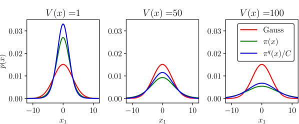
Figure 2: Normal Gaussian policy, $q$-Gaussian policy $\pi$ and $q$-escort distribution of $\pi^{q}/C$ policy with different value function.

III-C Sampling from q-escort distribution

In the forward pass of ME-DDP with Shannon entropy, a new control sequence is sampled from $\pi$ whose form is a Gaussian or a Gaussian mixture. In our case, since expectation of the cost is taken over the $q$-escort distribution of $q$-Gaussian $\pi$, it is more natural to sample from $\pi^{q}/C$ than from $\pi$. To sample from this distribution, we use the property of $q$- Gaussian, that is, the $q$-escort distribution of a $q$-Gaussian is also a $q$-Gaussian. To see this, let us introduce a parameter $q^{\prime}$ and a $q$-mean and covariance as follows.

$$q^{\prime}=2-\frac{1}{q},\ \mu^{\prime}=\mu_{q},\ \Sigma_{q}^{\prime}=\frac{n_{u}+2-n_{u}q}{n_{u}+(2-n_{u})q}\Sigma_{q}.$$ (19)

With these, consider a $q$-Gaussian PDF parameterized by $q^{\prime}$ as

$$p_{q^{\prime}}(x)$$

$$=\frac{1}{Z_{q^{\prime}}}\Big{[}1-\frac{1-q^{\prime}}{n_{u}+2-n_{u}q^{\prime}}(x-\mu_{q}^{\prime})^{\mathsf{T}}[\Sigma_{q}^{\prime}]^{-1}(x-\mu_{q}^{\prime})\Big{]}^{\frac{1}{1-q^{\prime}}},$$

By substituting (19) in, we see that $p_{q^{\prime}}(x)$ is proportional to

$$\Big{(}\Big{[}1-\frac{1-q}{n_{u}+2-n_{u}q}(x-\mu_{q})^{\mathsf{T}}\Sigma_{q}^{-1}(x-\mu_{q})\Big{]}^{\frac{1}{1-q}}\Big{)}^{q},$$ (20)

which is a $q$ th power of $q$-Gaussian. This implies that sampling from the $q$-escort distribution $(p_{q}(x))^{q}/C$ is achieved by sampling from the $q$-Gaussian distribution $p_{q^{\prime}}(x)$ obtained by the transformation given in (19). Moreover, sampling from $q$-Gaussian is equivalent to sampling from Student’s $t$ distribution with the transformation in (5) [27]. We use the technique to sample from the $\pi^{q}/C$ in our algorithm.

Here, we analyze the difference between the optimal control policies of ME-DDP with Shannon and Tsallis entropy. With Shannon entropy, the covariance of Gaussian $\pi^{\star}$ is determined only by $\alpha Q_{uu}$ as in (11). On the other hand, with Tsallis entropy, the covariance is also affected by the value function as in (17). We can interpret this as follows. When the cost of the trajectory is low and thus $\tilde{V}(x)$ is low, the algorithm does not need to explore much because the current trajectory is already good. Therefore, the covariance for exploration is small. In the opposite case, the covariance is amplified by the large $\tilde{V}(x)$, which encourages exploration. To see this, we visualize the normal Gaussian policy, $q$-Gaussian policy $\pi$, and its $q$-escort distribution $\pi^{q}/C$ with a 2D state $x=[x_{1},x_{2}]^{\mathsf{T}}\in\mathbb{R}^{2},\alpha=10$ and a unit $Q_{uu}$ in Fig. 2. As shown in the top of the figure, the three panels correspond to three different $\tilde{V}(x)$ s. On the left, when $\tilde{V}(x)$ is small, $\pi^{q}$ is tighter than Gaussian. While the Gaussian policy remains the same shape, $\pi^{q}$ becomes heavy-tailed as $\tilde{V}(x)$ increases to the right. This means that the covarinace is properly scaled based on the cost of the trajectory, rather than scaled with the same scaling factor. Due to this property, we deduce that the generalized case has better exploration capability, which we validate in section IV.

The proposed algorithm is summarized in Alg. 1. It takes in $N$ nominal control sequences and performs optimization, outputting one pair of state control trajectories that achieve the lowest cost. In the implementation, we keep $Q_{uu}^{-1}$ as $\Sigma$ as in the case of ME-DDP with Shanon entropy and properly scale it when sampling control.

Input: $x_{0}:$ initial state, $u^{(1:N)}$, $\Sigma^{(1:N)}$, $K^{(1:N)}$

: initial sequence, $m:$ sampling frequency, $I$: max iteration, $q$: entropic index that satisfies (4) .

Result: $x^{(b)},u^{(b)},K^{(b)}$

Compute initial trajectory $(x_{0:T}^{(1:N)})$ and cost $J^{(1:N)}$.

for $i\leftarrow 0$ to $I$ do

       if $i\%m=0$ then

             $x^{(1)},u^{(1)},K^{(1)},\Sigma^{(1)},J^{(1)}\leftarrow$ lowest cost mode

            

            $\pi\leftarrow$ $q$-Gaussian($u^{(1)}$, $x^{(1)}$, $K^{(1)}$, $\Sigma^{(1)}$);

            

            for $n\leftarrow 2$ to $N$ in parallel do

                   $x^{(n)},u^{(n)},K^{(n)},J^{(n)}$

                   $\leftarrow$ Sample from $\pi^{q}/C$ with (18), (19) and sampling technique from Student’s $t$ distribution in [27].

             end for

            

       end if

      

      for $n\leftarrow 1$ to $N$ in parallel do

             $k^{(n)},K^{(n)},\Sigma^{(n)}\leftarrow$ Backward Pass

             $x^{(n)},u^{(n)},J^{(n)}\leftarrow$ Line Search.

       end for

      

end for

$b\leftarrow\operatorname*{arg\,min}_{n}J^{(n)}$

Algorithm 1 generalized ME-DDP

III-D Availability of multimodal policy

In ME-DDP with Shannon entropy, the multimodal policy is available due to the additive structure of the partition function, which is not the case with Tsallis entropy. Indeed, from the partition function in (16), we get

$$z =\int\Big{[}(q-1)\frac{Q}{C\alpha}+1\Big{]}^{-\frac{1}{q-1}}\mathrm{d}u$$

$$=\int\Big{[}1-(q-1)\Big{(}\frac{l(x,u)+V(x^{\prime})}{C\alpha}\Big{)}\Big{]}^{-\frac{1}{q-1}}\mathrm{d}u$$

$$=\int\exp_{q}\Big{(}\frac{-l(x,u)}{C\alpha}\Big{)}\otimes_{q}\exp_{q}\Big{(}\frac{-V(f(x,u))}{C\alpha}\Big{)}\mathrm{d}u$$

$$=\int r(x,u)\otimes_{q}z(f(x,u))\mathrm{d}u,$$

where $\otimes_{q}$ is $q$-product [25] that is not distributed

$$(a+b)\otimes_{q}c\neq a\otimes_{q}c+b\otimes_{q}c.$$

Therefore, $z$ is not written as a sum of $z^{(n)}$s, as opposed to the Shannon entropy case.

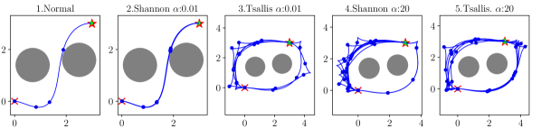
(a) 2D vehicle Example.

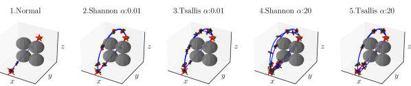
(b) Quadrotor Example.

Figure 3: Comparison of normal DDP, multimodal ME-DDP with Shannon entropy, and ME-DDP with Tsallis entropy with two different $\alpha$s. Trajectories of the 15 experiments are overlaid. $\times$ and $\bigstar$ indicate the initial and target positions, respectively. In the quadrotor example, obstacles are drawn in transparent.

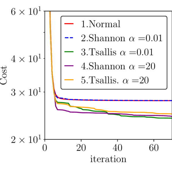
(a) 2D vehicle Example.

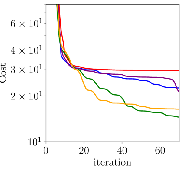
(b) Quadrotor Example.

Figure 4: Evolution of mean cost over iterations. The numbers in the legends corresponds to those in Fig.3

IV Numerical Experiments

In this section, we validate our proposed algorithm using two systems, a 2D car and a quadrotor. The tasks are to reach the targets while avoiding spherical obstacles which are encoded as part of the cost in (6). The cost for obstacles is given by

$$l_{\rm{s}}(x_{t})=\exp(-{(x_{t}-c_{\rm{o}})^{2}}/{2r_{\rm{o}}^{2}}),$$

where $c_{\rm{o}}$ and $r_{\rm{o}}$ are the center and radius of an obstacle, respectively. This cost structure is used in the original ME-DDP with Shannon entropy [21]. We first give a belief description of the systems and then give results of the experiment, including the comparison with a normal DDP without entropic regularization, ME-DDP with Shannon entropy, and our proposed ME-DDP with Tsallis entropy. In the experiment, we also examine the effect of the inverse temperature $\alpha$. Although ME-DDP by Shannon entropy has unimodal and multimodal versions, we only use the multimodal one for comparison because of its superior performance to the unimodal one. We note that ME-DDP with Tsallis entropy has a unimodal policy, as explained in the previous section. In both algorithms the number of trajectories is $N=8$.

IV-A 2D car

The state consists of the position and orientation $\theta$ of the car, and thus the state $x=[p_{x},p_{y},\theta]\in\mathbb{R}^{3}$. The control $u$ is translation and angular velocities $u=[v,\omega]\in\mathbb{R}^{2}$. In ME-DDP with Tsallis entropy, $q$ must satisfy $1<q<2$ from (4). We choose $q=1.6$. The control is initialized with all zeros.

IV-B Quadrotor

The state of the system consists of position, velocity, orientation, and angular velocity, all of which are $\mathbb{R}^{3}$, and thus $x\in\mathbb{R}^{12}$. The control $u$ of the system is the force generated by the four rotors, which gives $u\in\mathbb{R}^{4}$. The whole dynamics is found in [28]. The requirement for $q$ is $1<q<1.5$, and we choose $q=1.4$. The control sequence is initialized with all zeros.

IV-C Results

Fig. 3 shows the trajectories of the experiments with normal DDP, multimodal ME-DDP with Shannon entropy, and ME-DDP with Tsallis entropy (ours) with two different $\alpha$s. Experiments of ME-DDPs are performed 15 times, generating the same number of trajectories. Fig. 4 shows the evolution of the mean cost of experiments over optimization iterations.

In both dynamics, the normal DDP finds a local minimum that goes through between obstacles. However, ME-DDPs can explore and find better local minima that keep a greater distance from obstacles. ME-DDP with Shanon entropy requires a large $\alpha$ to explore (see 2s and 4s in Fig. 3). In fact, with a small $\alpha$, the results are almost the same as those of normal DDP in the 2D car example in Fig. 3(a) (1 and 2). This is because $\alpha$ determines the extent of exploration by scaling the variance of the policy. With generalized entropy, ME-DDP can explore well even with small $\alpha$s (see 3s and 5s). Although exploration is carried out with a unimodal policy in ME-DDP with Tsallis entropy, its exploration capability is better or equivalent to the multimodal policy of ME-DDP with Shannon entropy. This is the effect of the heavy-tailed shape of $q$-Gaussian and the value function on variance (17) analyzed in the previous section. Even with a small $\alpha$, the value function amplifies the variance for exploration when the cost of the trajectory is high, encouraging exploration. Due to this property, tuning $\alpha$ of generalized ME-DDP is relatively easy because one can simply choose a small $\alpha$, rather than finding a good $\alpha$. With a large $\alpha$ ME-DDP with generalized entropy fails to find a good local minimum which it used to find (see 3s and 5s in Fig. 4). We speculate that this is because the variance is scaled too much with both the $\alpha$ and the value function, making the exploration process difficult to sample meaningful trajectories. We have observed that the ME-DDP with Shanon entropy has the same tendency with too large $\alpha$ during the experiment.

V Conclusion

In this paper, we derived ME-DDP with Tsallis entropy. The algorithm has $q$-Gaussian policy whose variance is scaled not only by the inverse temperature parameter $\alpha$, but also by the value function of the trajectory being optimized. The results show that our algorithm can find better local minima in problems with multiple local minima even with a small inverse temperature parameter $\alpha$ compared to the original ME-DDP with Shannon entropy.

Future work includes hardware implementation of the proposed algorithms, as well as theoretical proofs such as the rate and condition of convergence. We are also interested in deriving ME-DDP with different entropy such as Rényi entropy.

References

- [1] C. Tsallis, “Possible generalization of boltzmann-gibbs statistics,” Journal of Statistical Physics, vol. 52, no. 1, pp. 479–487, Jul 1988. [Online]. Available: https://doi.org/10.1007/BF01016429
- [2] T. Leinster, Entropy and Diversity: The Axiomatic Approach. Cambridge University Press, 2021.
- [3] C. Tsallis, M. Gell-Mann, and Y. Sato, “Asymptotically scale-invariant occupancy of phase space makes the entropy sq extensive,” Proc Natl Acad Sci U S A, vol. 102, no. 43, pp. 15 377–15 382, Oct. 2005.
- [4] S. Umarov, C. Tsallis, and S. Steinberg, “On a q-central limit theorem consistent with nonextensive statistical mechanics,” Milan Journal of Mathematics, vol. 76, no. 1, pp. 307–328, Dec 2008. [Online]. Available: https://doi.org/10.1007/s00032-008-0087-y
- [5] E. Lutz, “Anomalous diffusion and tsallis statistics in an optical lattice,” Phys. Rev. A, vol. 67, p. 051402, May 2003. [Online]. Available: https://link.aps.org/doi/10.1103/PhysRevA.67.051402
- [6] B. Liu and J. Goree, “Superdiffusion and non-gaussian statistics in a driven-dissipative 2d dusty plasma,” Phys. Rev. Lett., vol. 100, p. 055003, Feb 2008. [Online]. Available: https://link.aps.org/doi/10.1103/PhysRevLett.100.055003
- [7] C. Bishop, Pattern Recognition and Machine Learning. Springer, January 2006. [Online]. Available: https://www.microsoft.com/en-us/research/publication/pattern-recognition-machine-learning/
- [8] C. Tsallis, S. V. F. Levy, A. M. C. Souza, and R. Maynard, “Statistical-mechanical foundation of the ubiquity of lévy distributions in nature,” Phys. Rev. Lett., vol. 75, pp. 3589–3593, Nov 1995. [Online]. Available: https://link.aps.org/doi/10.1103/PhysRevLett.75.3589
- [9] D. Prato and C. Tsallis, “Nonextensive foundation of lévy distributions,” Phys. Rev. E, vol. 60, pp. 2398–2401, Aug 1999. [Online]. Available: https://link.aps.org/doi/10.1103/PhysRevE.60.2398
- [10] N. Inoue and K. Shinoda, “q-gaussian mixture models for image and video semantic indexing,” Journal of Visual Communication and Image Representation, vol. 24, no. 8, pp. 1450–1457, 2013. [Online]. Available: https://www.sciencedirect.com/science/article/pii/S1047320313001855
- [11] D. Ghoshdastidar, A. Dukkipati, and S. Bhatnagar, “q-gaussian based smoothed functional algorithms for stochastic optimization,” in 2012 IEEE International Symposium on Information Theory Proceedings, 2012, pp. 1059–1063.
- [12] R. Tinós and S. Yang, “Use of the q-gaussian mutation in evolutionary algorithms,” Soft Computing, vol. 15, no. 8, pp. 1523–1549, Aug 2011. [Online]. Available: https://doi.org/10.1007/s00500-010-0686-8
- [13] T. Haarnoja, H. Tang, P. Abbeel, and S. Levine, “Reinforcement learning with deep energy-based policies,” in Proceedings of the 34th International Conference on Machine Learning - Volume 70, ser. ICML’17. JMLR.org, 2017, p. 1352–1361. [Online]. Available: https://api.semanticscholar.org/CorpusID:11227891
- [14] B. D. Ziebart, “Modeling purposeful adaptive behavior with the principle of maximum causal entropy,” Ph.D. dissertation, Carnegie Mellon Univ., 2010. [Online]. Available: https://www.cs.cmu.edu/~bziebart/publications/thesis-bziebart.pdf
- [15] G. Williams, N. Wagener, B. Goldfain, P. Drews, J. M. Rehg, B. Boots, and E. A. Theodorou, “Information theoretic mpc for model-based reinforcement learning,” in 2017 IEEE International Conference on Robotics and Automation (ICRA), 2017, pp. 1714–1721. [Online]. Available: https://ieeexplore.ieee.org/document/7989202
- [16] Z. Wang, O. So, J. Gibson, B. Vlahov, M. S. Gandhi, G.-H. Liu, and E. A. Theodorou, “Variational inference mpc using tsallis divergence,” in Robotics Science and Systems (RSS), 2021. [Online]. Available: https://www.roboticsproceedings.org/rss17/p073.pdf
- [17] G. Chen, Y. Peng, and M. Zhang, “Effective exploration for deep reinforcement learning via bootstrapped q-ensembles under tsallis entropy regularization,” 2018.
- [18] K. Lee, S. Kim, S. Lim, S. Choi, and S. Oh, “Tsallis reinforcement learning: A unified framework for maximum entropy reinforcement learning,” CoRR, vol. abs/1902.00137, 2019. [Online]. Available: http://arxiv.org/abs/1902.00137
- [19] L. Zhu, Z. Chen, E. Uchibe, and T. Matsubara, “Enforcing kl regularization in general tsallis entropy reinforcement learning via advantage learning,” 2022.
- [20] D. H. Jacobson and D. Q. Mayne, Differential dynamic programming. Elsevier, 1970.
- [21] O. So, Z. Wang, and E. A. Theodorou, “Maximum entropy differential dynamic programming,” 2022. [Online]. Available: https://arxiv.org/abs/2110.06451
- [22] L.-Z. Liao and C. Shoemaker, “Convergence in unconstrained discrete-time differential dynamic programming,” IEEE Transactions on Automatic Control, vol. 36, no. 6, pp. 692–706, 1991. [Online]. Available: https://ieeexplore.ieee.org/document/86943
- [23] W. J. Thistleton, J. A. Marsh, K. Nelson, and C. Tsallis, “Generalized box–mÜller method for generating -gaussian random deviates,” IEEE Transactions on Information Theory, vol. 53, no. 12, pp. 4805–4810, 2007. [Online]. Available: https://ieeexplore.ieee.org/document/4385787
- [24] C. Vignat and A. Plastino, “Poincaré’s observation and the origin of tsallis generalized canonical distributions,” Physica A: Statistical Mechanics and its Applications, vol. 365, no. 1, pp. 167–172, 2006, fundamental Problems of Modern Statistical Mechanics. [Online]. Available: https://www.sciencedirect.com/science/article/pii/S0378437106000744
- [25] ——, “Central limit theorem and deformed exponentials,” Journal of Physics A: Mathematical and Theoretical, vol. 40, no. 45, p. F969, oct 2007. [Online]. Available: https://dx.doi.org/10.1088/1751-8113/40/45/F02
- [26] Student, “The probable error of a mean,” Biometrika, vol. 6, no. 1, pp. 1–25, 1908. [Online]. Available: http://www.jstor.org/stable/2331554
- [27] D. Ghoshdastidar, A. Dukkipati, and S. Bhatnagar, “Smoothed functional algorithms for stochastic optimization using q-gaussian distributions,” ACM Trans. Model. Comput. Simul., vol. 24, no. 3, jun 2014. [Online]. Available: https://doi.org/10.1145/2628434
- [28] T. Luukkonen, “Modelling and control of quadcopter,” Independent research project in applied mathematics, Espoo, 2011. [Online]. Available: https://sal.aalto.fi/publicaitons/pdf-files/eluu11_public.pdf