On the Statistical Analysis of the Multipath Propagation Model Parameters for Power Line Communications

Abstract

This paper proposes a fitting procedure that aims to identify the statistical properties of the parameters that describe the most widely known multipath propagation model (MPM) used in power line communication (PLC). Firstly, the MPM parameters are computed by fitting the theoretical model to a large database of single-input-single-output (SISO) experimental measurements, carried out in typical home premises. Secondly, the determined parameters are substituted back into the MPM formulation with the aim to prove their faithfulness, thus validating the proposed computation procedure. Then, the MPM parameters properties have been evaluated. In particular, the statistical behavior is established identifying the best fitting distribution by comparing the most common distributions through the use of the likelihood function. Moreover, the relationship among the different paths is highlighted in terms of statistical correlation. The identified statistical behavior for the MPM parameters confirms the assumptions of the previous works that, however, were mostly established in an heuristic way.

I Introduction

The increasing demand of high-speed multimedia services led to reconsider the power delivery network as a data transmission medium. The PLC technology is becoming an established solution since it exploits the existing wired infrastructure to convey high-speed data content, thus saving costs and deployment time. Furthermore, the development of new standards and devices allows advanced signal processing and enhanced transmission techniques, such as the exploitation of all the deployed network conductors and the bandwidth extension, that improve even further the achievable data rate, guaranteeing transmission rates in the order of gigabit per second at the physical layer [1]. This high performance level motivates a renewed interest in developing novel and updated PLC solutions, especially for home networking and smart grid applications [2]. Since the main aim is to support the technological growth, it is fundamental to provide effective models, which are able to numerically emulate all the properties of an actual PLC network, thus avoiding on field tests. Two basic approaches can be tackled in defining a model, i.e., bottom-up and top-down, and both of them can follow a deterministic or a statistical strategy. A deterministic strategy typically considers a specific network configuration, while a statistical strategy attempts to introduce some variability by means of statistical distributions. Concerning the possible approaches, the bottom-up method has a strong physical connection and describes the phenomena involved in the signal propagation by exploiting the transmission line theory. Typically, it provides a faithful channel representation, although it turns out to be a computationally onerous procedure. Some examples concerning the SISO channel modeling can be found in [3], which proposes a deterministic approach, and in [4], which follows a statistical approach. While, recently, the models discussed in [5] and [6] extends the SISO bottom-up strategy to the multiple-input multiple-output (MIMO) transmission. Conversely, the topdown approach is an empirical method that fits an analytic function to a measurements database. This strategy facilitates the statistical extension by adopting a certain distribution for the parameters that describe the theoretical function. One of the first and more common SISO models is the MPM proposed in [7], which can be statistically extended as discussed in [8]. Instead, some MIMO models are presented in [9] and recently in [10], which extends the SISO formulation in [7] to the MIMO case.

I-A Contribution

The top-down MPM model formulated in [7] has been widely adopted as a reference model for the PLC scenario. Indeed, in order to emulate the typical PLC channel variability, many scientific contributions propose a model extension also to the MIMO context, by adopting several heuristic approaches. Thus, the intent of this paper is to provide an unified procedure that aims to establish the proper statistics for all the parameters of the well-known MPM proposed in [7] by fitting the theoretical model to a measurements database. The procedure considers 432 experimental channels measured in several European countries in-home networks that were analyzed in [11]. Part of this collection was previously presented in [10], and the results are consistent with the ones obtained from other extensive measurements in Italy that were characterized in [12]. The fundamental goal is to identify the right statistics for the MPM parameters. Unlike the a posteriori parameters inference discussed in[8], this paper aims to evaluate the intrinsic MPM parameter properties by analyzing them after an accurate channel-by-channel fitting. As it will be discussed, the obtained statistical distributions confirm part of the assumptions made in [8], or show some deviations. These properties will support the development of novel models or the refinement of existent ones, such as [10] that is based on the MPM.

I-B Notation

We use matrices and vectors denoted in regular boldface, the former in capital letters. Thus, the vector representing the channel frequency response (CFR) measurements is denoted as $\mathbf{h}$, and the fitted CFR vector is denoted as $\mathbf{\widehat{h}}$. The notation $\mathbf{a}(j)$ stands for the $j$-th component in $\mathbf{a}$ while $\mathbf{a}(i:j)$ denotes a vector comprising the elements of $\mathbf{a}$ from position $i$ to $j$. Similarly, $\mathbf{A}(:,i:j)$ represents a submatrix of $\mathbf{A}$ formed by taking all its rows and columns from $i$ to $j$ and $[\mathbf{A}(:,i),\mathbf{A}(:,j)]$ denotes a block matrix formed by matrices $\mathbf{A}(:,i)$ and $\mathbf{A}(:,j)$. The diagonal matrix $\mathbf{A}$ formed by placing the elements of vector $\mathbf{a}$ in the diagonal is denoted as $\mathbf{A}=\text{diag}(\mathbf{a})$. The Hermitian and transpose operators are represented as $(\cdot)^{\textrm{H}}$ and $(\cdot)^{\textrm{T}}$, respectively, and $|\cdot|$ stands for the amplitude.

I-C Organization

The paper is organized as follows. First, the MPM is briefly recalled in Section II. Second, the assumptions and the strategy adopted to evaluate the MPM parameters is detailed and justified in Section III. Then, the computed parameters properties, such as the statistical behavior and the exhibited relationship, are discussed for all the MPM describing parameters in Section IV. Finally, the conclusions follow in Section V.

II Multipath Propagation Model

The main aim of this paper is to establish the statistics of the MPM that has been originally presented in [7]. The MPM follows a top-down approach and describes the multipath propagation of the power signal into the PLC medium that is due to the line discontinuities, such as branches, or unmatched loads. As demonstrated in [7], and later adopted in [8], the analytic formulation of the CFR, which takes into account the multiple reflections occurring within a PLC network, is given as

$$\centering H\left(f\right)=A\sum_{i=1}^{N}{g_{i}}e^{-(a_{0}+a_{1}f^{K})d_{i}}e^{-j2\pi fd_{i}/v}\@add@centering$$ (1)

where $a_{0}$ and $a_{1}$ are the attenuation coefficients, while $g_{i}$ and $d_{i}$ are the path gain and the path length of the $i$-th path, respectively. Moreover, $A$ is a normalization coefficient that allows the adjustment of the channel attenuation, $N$ is the number of significant paths and $K$ is the exponent of the attenuation factor related to the cable features. Typical values of $K$ range between 0.5 and 1 [7], hence $K$ is assumed equal to one for the rest of this paper. The parameter $\nu=c\epsilon_{r}$ is the propagation speed of light in the cables, where $c$ is the speed of light in the vacuum and $\epsilon_{r}$ is the relative dielectric constant of the insulator which envelops the conductors. As specified in [8], in order to take into account the non-uniformity of the dielectric, it has been assumed $\epsilon_{r}=1.5$. The expression in (1) can be adopted as an analytic model that can be statistically extended in order to describe the variability encountered in a real communication scenario by imposing the proper properties to its describing parameters, such as the statistics and the exhibited relationship. Thus, the MPM parameters distribution and the correlation degree are established according to the procedure described in Section III.

III MPM Paramenter Evaluation Procedure

In order to provide a statistical characterization for the parameters that describe the MPM formulation in (1), the first step is to compute the MPM parameters by fitting the analytic expression to a set of experimental channels. In particular, a database of $432$ indoor channel frequency responses measured in different European countries using a vector network analyzer is herein considered [11]. The selected frequency band ranges from $1$ to $80$ MHz with a resolution of $\Delta f$= 61.875 kHz, resulting in $M=1277$ frequency samples.

Since the model is described by many parameters, some assumptions must be adopted in order to simplify the evaluation strategy, as it is detailed in the following. First, the positive range between 0 and $L$, i.e., the maximum possible length, for the initial possible path length values is discretized yielding uniformly spaced distances. This is a viable assumption since PLC networks typically exhibit a complex topology, with a great number of branches, especially concerning the indoor scenario. This results into approximately uniformly distributed distances traveled by the signal and its reflections from the transmitter side towards the receiver outlet. Thus, the set of possible path lengths is initially defined as

$$d_{i}\in n\frac{L}{N}\quad\text{with }n=0,...,N-1.$$ (2)

After the decimation procedure discussed in Section III-A, the survived dominant paths, i.e., the paths that actively contribute to the received signal, can be any possible combination of the above mentioned set, as it will be detailed. Afterwards, the attenuation coefficients $a_{0}$ and $a_{1}$ are established through the robust regression fit of each channel measurement, as follows. The channel attenuation, or path loss (PL), profile is strongly affected by the longest path. Thus, the contribution of the longest path in (1) is considered by imposing $N$ = 1 for the last (longest) path selection with $d_{1}=L$, i.e., the maximum distance, and this longest path distance is selected as

$$L=(M-1)\frac{v}{f_{M-1}-f_{0}}.$$ (3)

where the frequency values $f_{0}$ and $f_{M-1}$ correspond to the lowest and highest ones in the band of interest. The path lengths are assumed sorted by ascending order with $i$, without loss of generality. Furthermore, the corresponding path gain $g_{1}$ is assumed equal to one since it represents only a normalization coefficient that shifts the robust fit up or down, but does not affect its slope. According to the formulation in (1), the robust regression fit is inferred as

$$10\log_{10}|H(f)|^{2}=-2(a_{0}+a_{1}f)L\cdot 10\log_{10}e=\alpha_{0}+\alpha_{1}f,$$ (4)

where $\alpha_{0}$ and $\alpha_{1}$ are the coefficients of the robust regression fit. Thus, the attenuation coefficients are computed as

$$a_{0}=-\frac{\alpha_{0}}{20L\log_{10}e},a_{1}=-\frac{\alpha_{1}}{20L\log_{10}e}$$ (5)

The most straightforward method to determine the $g_{i}$, with $i=1,...,N$, would be to minimize the root mean square error (RMSE) w.r.t. the channel measurement given by

$$RMSE=\sqrt{\frac{1}{M}\sum_{m=0}^{M-1}{|H(f_{m})-\hat{H}(f_{m})|^{2}}},$$ (6)

where $H(f_{m})$ and $\widehat{H}(f_{m})$ represent the measured and fitted CFR at frequency $f_{m}$, respectively, being $M$ the number of frequency samples as above mentioned.

For the computation, the parameter $A$ could be assumed to be equal to 1 and, considering the Hermitian part in order to obtain real path gains, the expression in (1) for frequencies $f_{m}=f_{0}+m\Delta f$ with $f_{0}=1.0$ MHz and $0\leq m\leq M-1$ can be expressed by using matrices as

$$\underbrace{\begin{bmatrix}H(f_{0})\\ \vdots\\ H(f_{M-1})\\ H^{*}(f_{M-1})\\ \vdots\\ H^{*}(f_{0})\\ \end{bmatrix}}_{\mathbf{h}}=\underbrace{\begin{bmatrix}P_{0,0}&\dots&P_{0,N-1}\\ \vdots&&\vdots\\ P_{M-1,0}&\dots&P_{M-1,N-1}\\ P^{*}_{M-1,0}&\dots&P^{*}_{M-1,N-1}\\ \vdots&&\vdots\\ P^{*}_{0,0}&\dots&P^{*}_{0,N-1}\\ \end{bmatrix}}_{\mathbf{P}}\underbrace{\begin{bmatrix}g_{1}\\ \vdots\\ g_{N}\end{bmatrix}}_{\mathbf{g}}$$ (7)

where $P_{m,i}=\exp(-(a_{0}+a_{1}f_{m}^{K})d_{i})\cdot\exp(-j2\pi f_{m}d_{i}/v)$.
Hence, expression (7) can be compactly rewritten as $\mathbf{h}=\mathbf{P}\mathbf{g}$ and the path gains for each considered realization can be computed as

$$\mathbf{g}=\left(\mathbf{P}^{\textrm{H}}\mathbf{P}\right)^{-1}\mathbf{P}^{\textrm{H}}\mathbf{h},$$ (8)

which corresponds to a least squares (LS) estimation. However, an alternative method is chosen here, since the LS error is highly dominated by points with low attenuation, resulting in highly accurate fittings at these points, but, as attenuation increases, the accuracy significantly deteriorates. Hence, in order to achieve a balanced error distribution along the entire frequency band, since usually the higher the frequencies the higher the attenuation, we propose to obtain the path gain vector $\mathbf{g}$ using a weighted least squares (WLS) method for each considered realization, with a weight vector $\mathbf{w}=[1/|H(f_{0})|,1/|H(f_{1})|,\ldots,1/|H(f_{M-1})|,1/|H(f_{M-1})|,\ldots,\\ 1/|H(f_{1})|,1/|H(f_{0})|]^{T}$, by means of

$$\mathbf{g}=\left(\mathbf{P}^{\textrm{H}}\mathbf{W}\mathbf{P}\right)^{-1}\mathbf{P}^{\textrm{H}}\mathbf{W}\mathbf{h},$$ (9)

where $\mathbf{W}=\text{diag}(\mathbf{w})$.

III-A Dominant Paths Selection Procedure

In order to determine only the dominant paths that effectively contribute to the signal observed at the receiver side, the following decimation procedure is performed. The aim is to reduce the number of describing paths by deleting the less significant ones, but still providing a good approximation in terms of RMSE.

The set of path lengths was defined in (2) and the longest path length in (3), then $N$ will be the resulting decimated number of paths that is initially computed as (this value will be discussed later)

$$N=\frac{2f_{M-1}L}{v}.$$ (10)

The decimation procedure iteratively discards the path with the smallest contribution to approximate the measured CFR, while the remaining paths still provide a good approximation, according to a metric for the goodness of fit. Mathematically, the index of the path to be disregarded at each iteration, denoted as $p$, is selected according to the following criterion

$$p=\operatorname*{arg\,min}_{i}{\left\{\bigg{|}\sum_{m}g_{i}\cdot\exp(-(a_{0}+a_{1}f_{m})d_{i})\bigg{|}\right\}}.$$ (11)

The rationale for this criterion is that the actual contribution of a path to the overall CFR is essentially determined by the factor $g_{i}\cdot\exp(-(a_{0}+a_{1}f)d_{i}$ in the MPM in (1). The metric adopted for the decimation procedure is the normalized root mean square error (NRMSE), given by

$$NRMSE=\sqrt{\frac{1}{M}\sum_{m=0}^{M-1}{\frac{|H(f_{m})-\hat{H}(f_{m})|^{2}}{|H(f_{m})|^{2}}}},$$ (12)

which aligns with the introduction of the WLS method, as the employed weight vector is designed to minimize the NRMSE. It is assumed that if the metric in dB is less than a fixed value, equal to -15 dB in the evaluation process, it means that the channel computed with a reduced set of paths still represents a very good approximation of the corresponding measurement.

Thus, essentially the selection procedure involves the elimination of the path related to the minimum path gain factor in absolute value in (11). This is deleted by removing the corresponding column of the matrix $\mathbf{P}$. The elimination process is cyclically repeated until the metric in dB exceeds the imposed limit and so the precision is preserved. When the selection procedure is terminated, the path gains obtained for the considered measurement, which are determined assuming $A$=1, are normalized by their maximum absolute value. This normalization factor provides the value for the parameter $A$. This way, the $g_{i}$ values that represent the product of transmission and reflection coefficients, which are always less then one in magnitude, belong to the [-1,1] interval [7]. While, the normalization coefficient $A$ for the given realization belongs to the interval [0,1]. Nevertheless, to summarize, Table I presents the fitting and decimation procedure in more detail.

Table I: Algorithm of the fitting and path selection procedure

Algorithm: MPM fitting procedure

Input: $\mathbf{h}$, $\widehat{\mathbf{h}}$

1: Compute $L=(M-1)v/(f_{M-1}-f_{0})$

2: Compute $a_{0}$ and $a_{1}$ using (5)

3: Compute $N=2f_{M-1}L/v$

4: Initialize $\mathbf{d}=iL/N$ with $i=0,...,N-1$

5: Initialize $\mathbf{g}$ using (9)

6: Compute $\mathbf{\widehat{h}}$ using (1)

7: Compute the NRMSE using (12)

8: while $\acs{NRMSE}<-15$ do

9: Compute $p$ using (11)      10: Perform $\mathbf{P}=[\mathbf{P}(:,0:p-1),\mathbf{P}(:,p+1:N-1)]$      11: Update $\mathbf{g}$ using (9)      12: Compute $\widehat{\mathbf{h}}$ using (1)      13: Compute the NRMSE using (12)      14: Compute $N=N-1$

15: end while

16: Compute $\mathbf{P}=[\mathbf{P}(:,0:p-1),\mathbf{P}(:,p),\mathbf{P}(:,p+1:N-1)]$

17: Compute $\mathbf{g}=[\mathbf{g}(0:p-1),\mathbf{g}(p),\mathbf{g}(p+1:N-1)]$

Indeed, the reconstructed channel realizations from the model are extremely accurate since the initial $NRMSE_{dB}$, computed before the paths selection procedure, shows an average and standard deviation values equal to $\mu_{dB}$=-37.63 dB and $\sigma_{dB}$=7.99 dB, respectively. The number of paths considered for the model at this pre-decimation point is of 2584. After the application of the proposed procedure, the number of paths has been decimated to get a mean value of 167.48 paths for the whole set of measurements and the corresponding statistical values of the $NRMSE_{dB}$ is equal to $\mu_{dB}$=-15.17 dB and $\sigma_{dB}$=0.21 dB. Hence, there is a good trade-off between the modeling complexity and its accuracy.

For illustrative purposes, in Fig.1 a typical experimental measurement of the CFR $H(f)$ is shown, extracted from the considered database, exhibiting the good fit with the reconstructed channel $\hat{H}(f)$, i.e., generated according to the multipath propagation model in (1) by using the computed parameters. Only the dominant paths survived from the decimation process are used for the computation, which correspond $N$=294 paths for the specific case in Fig.1. Both the channel amplitude response in dB scale and the corresponding channel unwrapped phase are represented. As can be observed, the measured trace is almost veiled by the estimated one because the fitting accuracy. As clarified in Fig.1, the computed parameters allow a faithful CFR reconstruction through the MPM, despite the reduced number of paths. Thus, the MPM parameters can be evaluated for each distinct measurement according to the procedure described within this section. There are only two additional quantities to be fixed, the maximum length $L$ and the maximum number of initial possible paths $N$. These parameters cannot be chosen arbitrarily, indeed, they depend among each other, as well as on the number of frequency samples, as described in the following section.

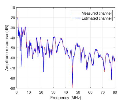
(a)

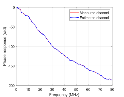
(b)

Figure 1: Amplitude (a) and phase (b) fittings obtained via the proposed MPM after selecting a reduced set of 294 significant paths for an illustrative measurement.

III-B Relation among L, M, and N

The maximum length $L$, the maximum number of paths $N$, and the number of frequency samples $M$ depend among each other and must satisfy certain constraints. Since a discrete and finite number of frequencies is available, the expression in (1) given for the continuous frequency domain can be rewritten for the discrete domain as

$$H(f_{m})=A\sum_{n=0}^{N-1}r_{n}e^{-j2\pi m\Delta fnL/N_{\nu}},$$ (13)

where $\Delta f=(f_{M-1}-f_{0})/(M-1)$ is the frequency resolution, while $\tau=L/N_{\nu}$ is the time resolution. Note that in (13) the path index $n$ belongs to $[0,...,N-1]$, differently from (1), where $i$ assumes values in $[1,...,N]$. Furthermore, the real part of the exponential term has been embedded within the corresponding path gain in a unique variable named $r_{n}$. The adopted notation does not affect the analysis since the real exponential part acts only as an attenuation term that increases with frequency.

The equation in (13) can be seen as a discrete time Fourier transform (DFT) with frequency index $m$ and time index $n$. As known, the DFT assumes the time signal belonging to domain of integer multiples of $\tau$ and periodic of $N\tau$. Such a domain is denoted with $\mathbb{Z}(\tau)/\mathbb{Z}(N\tau)$. Hence, in the frequency domain the signal is defined in $\mathbb{Z}(\Delta f)/\mathbb{Z}(N\Delta f)$, with $\Delta f=1/(N\tau)$. Therefore, the relation between $L$ an the frequency samples $M$ is given by

$$\Delta f=\frac{f_{M-1}-f_{0}}{M-1}=\frac{1}{N\frac{L}{N\nu}}=\frac{\nu}{L}\Rightarrow L=\frac{(M-1)\nu}{f_{M-1}-f_{0}}$$ (14)

Since the measurements span the 1–80 MHz band, i.e., $f_{M-1}=80$MHz and $f_{0}=1$MHz, with 1277 frequency samples and the propagation speed is $\nu=2\cdot 10^{8}$ m/s, the maximum possible length that can be assumed is $L=3190$ m. The limit of more than 3 kilometers turns out to be a maximum length that is long enough to describe any generic in-home network topology. Moreover, always referring to the DFT representation of the CFR reported in (13), the DFT frequency period, i.e., $N\Delta f$, must be greater or equal than two times the maximum channel frequency, i.e., $f_{M-1}$, in order to avoid aliasing problems according to the sampling theorem. Thus, the relationship among $N$ and $L$ turns out to be

$$N\Delta f=\frac{1}{\tau}\geq 2f_{M-1}\Rightarrow N\geq\frac{2f_{M-1}L}{\nu}.$$ (15)

If the aforesaid values for $f_{M-1}$ and $\nu$ are considered, the relation in (15) becomes $N\geq L$.

A final relation among $N$ and $L$ can be noticed by rewriting the imaginary part of the exponential term in (1) as

$$e^{-j2\pi fd_{i}/\nu}=e^{-j2\pi kd_{i}/\lambda}$$ (16)

where $\lambda=\nu/\Delta f$ is the maximum possible wavelength, which is related to the frequency resolution $\Delta f$. The minimum observable wavelength is $\lambda_{min}=\nu/f_{M-1}$. Hence, to avoid numerical errors, the shortest path length $d_{1}$ must be greater than $\lambda_{min}/2$, according to the sampling theorem. This provides the last relationship, expressed by

$$d_{1}=\frac{L}{N}\geq\frac{\lambda_{min}}{2}\Rightarrow N\leq\frac{2f_{M-1}L}{\nu}$$ (17)

It can be noted that, given the above mentioned specifications, as well as the relations (15) and (17), the relationship among $L$ and $N$ must hold with equality, i.e., $N=L=3190$, for the considered database.

IV MPM Parameter Properties

This section assesses the statistical properties of all the MPM parameters established according to the procedure detailed in Section III. The overall set of computed values, determined for each of the available channel measurements, are considered. Furthermore, since each channel measurement is described by a certain number $N$ of paths, yielding multiple path length and path gain values, it is fundamental to evaluate the relationship between the different $d_{i}$ and $g_{i}$ of the paths, with $i=[1,...,N]$, as well as between both these quantities. It is important to state that, without loss of generality, all the path lengths are considered in ascending order, according to their definition in (2). Thus, the higher the index, the longer the corresponding path. While, the path gains, which are related to the corresponding path length, are sorted accordingly.

IV-A Statistical Behavior

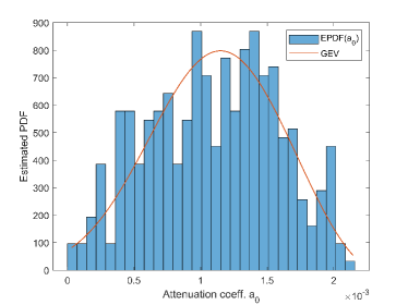
(a)

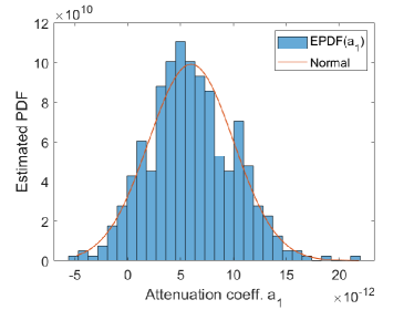
(b)

Figure 2: Estimated PDF (EPDF) of the attenuation coefficients $a_{0}$ and $a_{1}$.

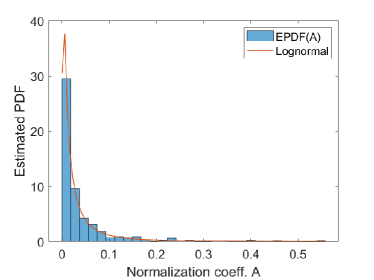
(a)

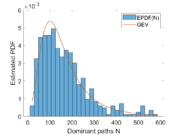
(b)

Figure 3: Estimated PDF of normalization coefficient $A$ and number of dominant paths $N$.

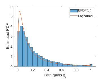
(a)

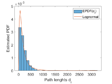
(b)

Figure 4: Estimated PDF of path gains $g_{i}$ and path lenghts $d_{i}$.

parameters, which have been computed through the evaluation procedure discussed in Section III, is assessed. In order to establish the best fitting pdf for the MPM parameters, the likelihood function is exploited. It is computed as [13]

$$\Lambda(\theta)=\prod_{x\in\mathbb{X}}p(x|\theta)$$ (18)

where $x\in\mathbb{X}$ is the set of measured samples, $p(\cdot)$ is the pdf of the fitting distribution, and $\theta$ represents the parameters of such distribution, obtained by the estimation. The higher the likelihood function score, the better the selected distribution fits the corresponding parameter data. The comparison is performed with the most common distribution functions, such as: beta, binomial, Birnbaum-Saunders exponential, gamma, generalized extreme value (GEV), generalized Pareto, Gumbel, inverse Gaussian, logistic, log-logistic, log-normal, Nakagami, negative binomial, normal, Poisson, Rayleigh, Rician, $t$ location-scale and Weibull.

The estimated pdf for each MPM parameter are reported in Fig. 2, 3 and 4. They are obtained by means of normalized histogram bar charts, so that the integral yields 1, together with the corresponding distribution function that shows the best likelihood score. It can be noted as each parameter exhibits its own experimental trend that can be fitted with a certain distribution function. In particular, the attenuation coefficients $a_{0}$ and $a_{1}$ exhibit a GEV and a normal distribution, respectively. In practice, the GEV is a family of three types of extreme value distributions, namely type I, or Gumbel [14], type II, or Fréchet, and type III, or Weibull distribution. This result makes sense since the GEV distribution models the maximum of long and finite sequences of random variables. The distribution for $a_{0}$ is justified since it represents the maximum (or the minimum) of a number of samples of various distributions. Indeed, $a_{0}$ corresponds to the maximum (or the minimum in case of negative values of $a_{1}$) PL value for the identified trend of each analyzed measurement. Differently, the normal pdf for $a_{1}$ represents the PL slope fluctuations among the positive and possibly negative values with an average more probable value.

The number of significant paths $N$ survived from the selection process discussed in Section III-A, shows also a GEV distribution. As a matter of fact, $N$ represents the maximum number of dominant paths that actively contribute to reconstruct each measurement.

Concerning the MPM parameters related to each different path that survived from the decimation process, namely $d_{i}$ and $g_{i}$, with $i=[1,...,N]$, it is found that both the path lengths ($d_{i}$) and the absolute value of the path gains ($|g_{i}|$) show an Log-normal distribution, despite the values of the latter are confined in $[0,1]$. These results hold at each frequency sample and for each considered path, as well as for the overall set of measurements. The absolute value of the path gains is considered since, from experimental evidence, they exhibit a specular distribution that is mirrored w.r.t. the $y$-axis, with values equally divided among positive and negative. Not only the path lengths and gains, but also the normalization coefficient $A$ turns out to be log-normally distributed, as expected for a PLC environment [15], [16], [12]. The pdfs of $|g_{i}|$ and $d_{i}$ obtained considering the overall set of values, regardless the frequency sample and the considered path, are depicted in Fig. 4.

All the computed MPM parameters distribution with the corresponding representative parameters value are summarized in Table II. The reported results will allow future replicability of this study and simplify the development of updated statistical models.

Table II: Estimated PDF fitting for MPM parameters

MPM parameter	Distribution	Dist. parameters
Atten. coeff. ($a_{0}$)	GEV	$k=-0.3593$ $\sigma=4.9661\cdot 10^{-4}$ $\mu=9.4529\cdot 10^{-4}$
Atten. coeff. ($a_{1}$)	Normal	$\mu=6.0018\cdot 10^{-12}$ $\sigma=4.0223\cdot 10^{-12}$
Norm. coeff. ($A$)	Log-normal	$\mu=-4.2001$ $\sigma=1.4261$
Dominant paths ($N$)	GEV	$k=0.1953$ $\sigma=69.6141$ $\mu=112.2569$
Path gains ($g_{i}$)	Log-normal	$\mu=-2.0701$ $\sigma=1.2407$
Path lengths ($d_{i}$)	Log-normal	$\mu=4.9351$ $\sigma=0.9518$

IV-B Comparison with Other Works

The above identified MPM parameter distributions are herein compared with those empirically defined in other scientific works. For example the statistical analysis performed in Section IV-A confirms the assumptions made in [8], which statistically extends the MPM in (1) relying on the initial idea presented in [17]. Indeed, as inferred in [8], the path gains $g_{i}$ turn out to be log-normally distributed variables multiplied by a random flip sign. While, the path lengths $d_{i}$ here, after the effective decimation procedure, appear to be log-normally distributed extending the tail up to the maximum lenght $L$. Additionally, the characterization method proposed in this paper provides a statistics for the other parameters, i.e., $a_{0}$, $a_{1}$, and $A$. The main difference is found for the statistics of $N$, supposed to have a Poisson distribution in [8], but that results into a GEV distribution. This difference was already hypothesized in [8] and is also justified by the different considered databases.

Other results concerning the MPM parameters distribution are listed in [18](Tab. 1), that extends the model in (1) to the MIMO transmission. In this case, the path gains $g_{i}$ are assumed uniformly distributed in [-1, 1] and the attenuation coefficient $a_{1}$ turns out to be constant. While, $K$ is normally distributed and $a_{0}$ exhibits a shifted exponential distribution. Instead, the channel median $A$ is uniformly or exponentially distributed depending on the considered channels. The same results are also summarized in [19](Tab. 2.10).

Beyond the parameters distribution characteristics, it is interesting to study the correlation for the path lengths and the path gains, exhibited among the different paths, as described in the following subsection. This is necessary in order to provide a complete characterization, which is able to represent all the effects encountered in a real communication scenario.

IV-C Exhibited Relationship

In order to provide a complete characterization of the MPM parameters in the expression in (1) it is of great importance to assess not only the statistical distribution, but also the degree of correlation for the path gains and the path lengths among different paths, as well as between each other. This is since there are multiple $g_{i}$ and $d_{i}$ values that describe each single realization. The statistical normalized covariance matrix, or Pearson correlation [20], is considered here in order to obtain values in [0, 1], where 0 stands for no correlation, while 1 means fully correlated. It is computed as

$$\mathbf{R}_{x}(i,j)=\frac{E[(x_{i}-\mu_{x_{i}})(x_{j}-\mu_{x_{j}})^{*}]}{\sigma_{x_{i}}\sigma_{x_{j}}}$$ (19)

where $\{i,j\}\in[1,...,N]$ are the path indexes, $E[\cdot]$ is the expectation operator performed over the realizations, while $x$ denotes the considered quantity, e.g. $g$, $d$, or their combination. Furthermore, $\mu_{x_{i}}$ and $\sigma_{x_{i}}$ are the mean and the standard deviation related to the $i$-th path. In practice, the quantity in (19) is the statistical covariance matrix normalized by the product of the corresponding paths standard deviation. For simplicity, in the following it is referred to as correlation matrix.

Since each measurement is reconstructed with a different number of paths N, there are two alternative ways to compute the correlation in (19). The first method involves the choice of a proper number of paths $N$ that is big enough to observe the correlation also with the longest paths (high indexes), but not too big in order to have a sufficient number of realizations that have such a large $N$ to provide good results for the correlation matrix computation. This is since the higher the considered number of paths, the lower the number of realizations that are reconstructed by an equal, or greater, number of paths, which can be used for the computation. The second method, instead, evaluates the correlation by exploiting all the measurements that have been reconstructed with a number of paths $N$ equal to, or grater than, the number of paths for which the correlation is computed, starting from the lowest obtained number $N$. This way, it is possible to compute the correlation among all the possible paths required for a faithful channel reconstruction in an incremental manner. Obviously, the values related to the high paths (indexes) are affected by a larger uncertainty due to the reduced set of available realizations that can be used in the computation.

This last method has been chosen for the correlation computation as in (19) since it provides a more complete information of the relationship among all the computed paths concerning both $g_{i}$ and $d_{i}$. However, the maximum number of displayed paths is fixed equal to 2500 in order to avoid to provide results of poor statistical significance, i.e., computed relying on few measurements.

The path gains correlation matrix ($\mathbf{R}_{g}$), computed as in (19), is reported in Fig. 5. It can be noted that the path gains exhibit a high correlation that increases for nearer paths, while decreases for far paths, although a significant level of correlation is exhibited almost everywhere. Relevant values of correlation are experimented also by the path gains with a low index, around 100 and 200, with almost all the others. Contrariwise, the higher the index, the lower the correlation with the other paths. If a simplification is desired, since a similar value of correlation is exhibited by equally spaced paths, the matrix $\mathbf{R}_{g}$ can be approximated with a Toeplitz matrix, which is a diagonal-constant matrix.

The experimental mean ($\mathbf{\mu}_{g}$) and the variance ($\mathbf{\sigma}^{2}_{g}$) of the path gains for each path, which have been computed by considering the overall measurements and according to the incremental procedure above described, are reported in Fig. 6. It can be noted that both $\mathbf{\mu}_{g}$ and $\mathbf{\sigma}^{2}_{g}$ profiles slightly decrease for low path indexes, with a minimum for the paths in the neighborhoods of the index $i$ = 500, while increase for high indexes. Furthermore, the variance profile is more noisier if compared to the mean profile, due to the high variability encountered in a real communication scenario. In this case the experimental profiles can be approximated via a polynomial function $p(x)$ of degree $n$, which provides the best fit in a least-squares sense, given by

$$p(x)=p_{n}x^{n}+p_{n-1}x^{n-1}+...+p_{1}x+p_{0},$$ (20)

where $x$ represents the support, e.g. the path index, while $p(x)$ is the approximated profile. All the quantities $p_{r}$, with $r=0,...,n$, are constant coefficients.

Table III: Parameters of the polynomial fit for the different quantities

Quantity	$p_{3}$ ($\times 10^{-9}$)	$p_{2}$ ($\times 10^{-6}$)	$p_{1}$ ($\times 10^{-3}$)	$p_{0}$
$\mathbf{\mu}_{g}$	-0.585	2.829	-2.401	-6.486
$\mathbf{\sigma}^{2}_{g}$	-0.262	1.454	-1.692	1.336

The approximated version of the $\mathbf{\mu}_{g}$ and $\mathbf{\sigma}^{2}_{g}$ trends is still represented in Fig. 6. Instead, the coefficients of the polynomial fits are reported in Table III. It can be noted that the experimental profiles are well fitted by the approximated profiles with only 4 coefficients.

The path lengths correlation matrix ($\mathbf{R}_{d}$), instead, is represented in Fig. 7. As shown, the $d_{i}$ values exhibit a significant level of correlation as well, especially for nearer paths. However, the longest the path (high index), the highest the correlation with the short ones. This is justified by the fact that the long distances (paths) traveled by the transmitted signal are multiple of the shortest ones. Also $\mathbf{R}_{d}$ can be approximated with Gaussian pdf profiles, normalized in [0, 1] and distributed orthogonality w.r.t. the main diagonal, with a varying variance. Although not shown for compactness, the correlation among the path gains and lengths, i.e., $\mathbf{R}_{g,d}$, exhibits very low values almost everywhere, namely always below 0,3, except some few coefficients. This is due to the prominent effect of the multipath propagation, which involves that the path gains associated to the corresponding path lengths exhibit an approximately random magnitude among the considered measurements.

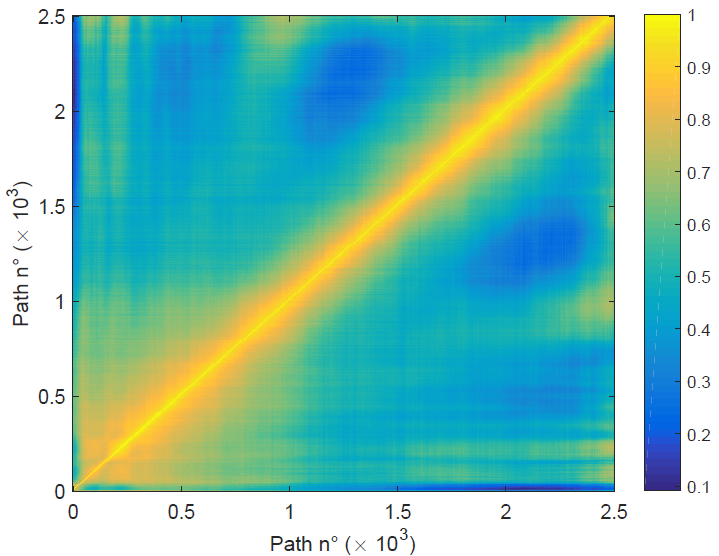
Figure 5: Path gains experimental correlation matrix up to 2500 paths.

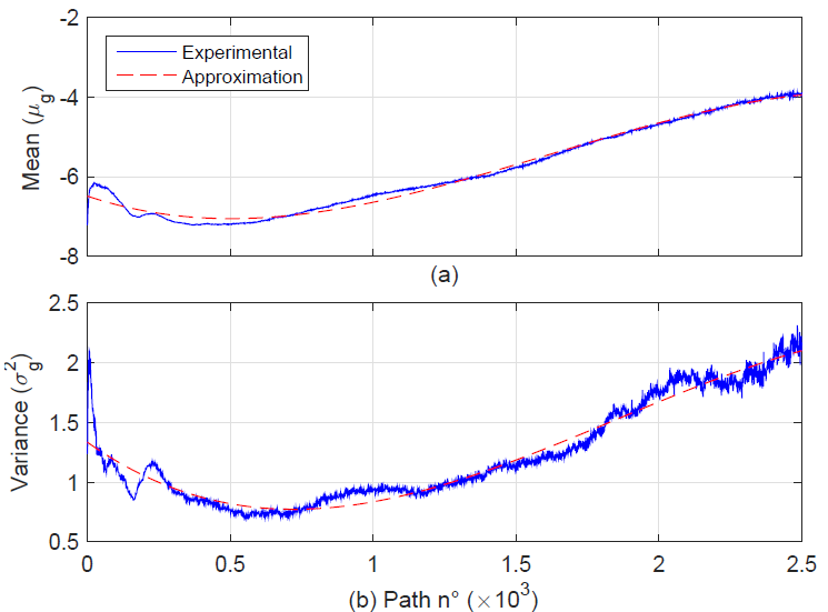
Figure 6: Mean (a) and variance (b) of the path gains at each path. The corresponding polynomial approximation is also shown.

Figure 7: Path lengths experimental correlation matrix up to 2500 paths.

V Conclusion

This paper considers one of the most common top-down models adopted in the literature, namely the multipath propagation model. Since the MPM formulation has been many times adopted as a reference model in PLC, or it has been statistically extended to different contexts, the aim has been to propose an unified approach to find out the statistical properties of its describing parameters. In order to provide a closed-form solution, due to the high number of parameters, some of them have been imposed on the basis of common sense intuition., while other parameters, such as the attenuation parameters and the set of initial path lengths, have been chosen according to physical assumptions. Then, when most of the parameters are fixed, the other ones, e.g. the path gains, can be analytically retrieved by matrix inversion.

Moreover, only the dominant paths that actively contribute to the CFR have been selected according to a proposed decimation procedure to yield a more compact modeling. The implemented selection method has allowed to establish also the amount of significant paths, discarding the less relevant ones, i.e., with the lowest gains, according to the RMSE. As a proof of the correctness of the determined values, the channel measurements have been reconstructed exploiting the identified values. The comparison exhibits a good agreement, despite the paths decimation. Finally, once that the MPM parameters have been computed according to the proposed strategy, their statistics has been established by means of the best likelihood fitting distribution. While, the relationship among the different path gains and lengths has also been evaluated, highlighting a non negligible degree of correlation. This way, it has been possible to provide a specific statistical distribution for all the MPM describing parameters, as well as a correlation degree, proposing a method to approximate the exhibited relationship. These information will aid the development of novel and updated models for PLC, enabling the results replicability.

VI Acknowledgments

This work has been partially supported by the Spanish Government under project PID2019-109842RBI00/AEI/10.13039/501100011033.

References

- [1] L. Yonge, J. Abad, K. Afkhamie, L. Guerrieri, S. Katar, H. Lioe, P. Pagani, R. Riva, D. M. Schneider, and A. Schwager, “An overview of the homeplug AV2 technology,” Journal of Electrical and Computer Engineering, vol. 2013, pp. 1–20, 2013.
- [2] S. F. Bush, S. Goel, G. Simard, I. C. Society, and I. S. Association., “IEEE vision for smart grid communications: 2030 and beyond roadmap,” IEEE Vision for Smart Grid Communications: 2030 and Beyond Roadmap, pp. 1–19, 2013.
- [3] S. Galli and T. C. Banwell, “A deterministic frequency-domain model for the indoor power line transfer function,” IEEE Journal on Selected Areas on Communications, vol. 24, pp. 1304–1316, 7 2006.
- [4] A. M. Tonello and F. Versolatto, “Bottom-up statistical PLC channel modeling Part I: Random topology model and efficient transfer function computation,” IEEE Transactions on Power Delivery, vol. 26, pp. 891–898, 2011.
- [5] F. Versolatto and A. M. Tonello, “An MTL theory approach for the simulation of MIMO power line communication channels,” IEEE Transactions on Power Delivery, vol. 26, pp. 1710–1717, 2011.
- [6] J. Corchado, J. Cortés, F. Cañete, and L. Díez, “An MTL-based channel model for indoor broadband MIMO power line communications,” IEEE Journal on Selected Areas in Communications, vol. 34 pp. 2045–2055, 2016.
- [7] M. Zimmermann and K. Dostert, “A multipath model for the powerline channel,” IEEE Transactions on Communications, vol. 50, pp. 553–559, 4 2002.
- [8] A. M. Tonello, F. Versolatto, B. Bejar, and S. Zazo, “A fitting algorithm for random modeling the PLC channel,” IEEE Transactions on Power Delivery, vol. 27, pp. 1477–1484, 2012.
- [9] A. Canova, N. Benvenuto, and P. Bisaglia, “Receivers for MIMO-PLC channels: Throughput comparison,” IEEE ISPLC 2010 - International Symposium on Power Line Communications and its Applications, pp. 114–119, 2010.
- [10] P. Pagani and A. Schwager, “A statistical model of the in-home MIMO PLC channel based on european field measurements,” IEEE Journal on Selected Areas in Communications, vol. 34, pp. 2033–2044, 7 2016.
- [11] I. Povedano, F. Crespo, F. Cañete, J. Cortés, and L. Díez, “A statistical model for indoor SISO PLC channels,” IEEE ISPLC 2023 - International Symposium on Power Line Communications and its Applications, pp.1–6, 2023.
- [12] A. M. Tonello, F. Versolatto, and A. Pittolo, “In-home power line communication channel: Statistical characterization,” IEEE Transactions on Communications, vol. 62, pp. 2096–2106, 2014.
- [13] P. J. Bickel and K. A. Doksum, Mathematical Statistics. Basic Ideas and Selected Topics. Chapman and Hall, CRC, 12, 2015.
- [14] E. J. Gumbel, Statistical Theory of Extreme Values and Some Practical Applications. A Series of Lectures. U.S. National Technical Reports Library. Applied mathematics series, 1954. [Online]. Available: https://ntrl.ntis.gov/NTRL/dashboard/searchResults/titleDetail/PB175818.xhtml
- [15] S. Galli, “A novel approach to the statistical modeling of wireline channels,” IEEE Transactions on Communications, vol. 59, pp. 1332–1345, 2011.
- [16] J. A. Cortés, F. J. Cañete, L. Díez, and J. L. G. Moreno, “On the statistical properties of indoor power line channels: Measurements and models,”IEEE ISPLC 2011 - International Symposium on Power Line Communications and its Applications 2011, pp. 271–276.
- [17] A. M. Tonello, “Wide band impulse modulation and receiver algorithms for multiuser power line communications,” EURASIP J. Adv. Signal Process., vol. 2007, 2007, article ID 96747.
- [18] R. Hashmat, P. Pagani, A. Zeddam, and T. Chonave, “A channel model for multiple input multiple output in-home power line networks,” IEEE ISPLC 2011 - International Symposium on Power Line Communications and Its Applications, ISPLC 2011, pp. 35–41, 2011.
- [19] L. Lampe, A. M. Tonello, and T. G. Swart, Eds., Power Line Communications: Principles, Standards and Applications from Multimedia to Smart Grid, 2nd ed. Wiley, 2016.
- [20] M. Gilli, D. Maringer, and E. Schumann, Numerical Methods and Optimization in Finance. Elsevier, 2019.