Convergence of Iterative Quadratic Programming for Robust Fixed-Endpoint Transfer of Bilinear Systems

Abstract

We present a computational method for open-loop minimum-norm control synthesis for fixed-endpoint transfer of bilinear ensemble systems that are indexed by two continuously varying parameters. We suppose that one ensemble parameter scales the homogeneous, linear part of the dynamics, and the second parameter scales the effect of the applied control inputs on the inhomogeneous, bilinear dynamics. This class of dynamical systems is motivated by robust quantum control pulse synthesis, where the ensemble parameters correspond to uncertainty in the free Hamiltonian and inhomogeneity in the control Hamiltonian, respectively. Our computational method is based on polynomial approximation of the ensemble state in parameter space and discretization of the evolution equations in the time domain using a product of matrix exponentials corresponding to zero-order hold controls over the time intervals. The dynamics are successively linearized about control and trajectory iterates to formulate a sequence of quadratic programs for computing perturbations to the control that successively improve the objective until the iteration converges. We use a two-stage computation to first ensure transfer to the desired terminal state, and then minimize the norm of the control function. The method is demonstrated for the canonical uniform transfer problem for the Bloch system that appears in nuclear magnetic resonance, as well as the matter-wave splitting problem for the Raman-Nath system that appears in ultra-cold atom interferometry.

I Introduction

The synthesis of open-loop optimal controls for bilinear dynamical systems has been studied for decades [1]. The bilinear dynamics in this setting are characterized by evolution equations that are linear ordinary differential equation (ODE) systems where some coefficients can be chosen as functions of time, and a minimum norm control input is typically desired. The so-called bilinear-quadratic problems that result have been addressed by iterative feedback control synthesis methods [2], and the approach has been extended to open loop controls for fixed-endpoint state transfers [3]. In practice, it is of interest to synthesize controls that are robust or insensitive to uncertainty or variation in system parameters, and this leads to infinite-dimensional systems [4]. State feedback is impractical or unavailable in this setting, and thus open-loop controls are sought. Control robustness is typically understood as a uniform state transfer effect on all dynamical units in an ensemble or collection of structurally-similar systems indexed by parameters varying on a compact set [3, 5]. The desired control solution will steer the entire ensemble from the initial state to within an allowable distance of the desired target state. Rigorous definitions and conditions under which ensemble controllability is assured have been established for ensemble systems that have certain bilinear structures [6, 5, 7, 8].

Interest in control synthesis methods for fixed-endpoint transfers of bilinear ensembles has been driven over the past decades by problems related to quantum control applications [9]. Several approaches to solve the associated optimal control problem (OCP) employ fixed-point iteration directly either using linearization and approximation by Freholm operators [10] or by solving the quadratic-bilinear Riccati problem [3]. A variety of methods have been proposed to approximate infinite-dimensional ensembles using finite-dimensional representations, which typically involves spectral approximation [11]. A promising recent concept involves so-called polynomial moments [12], in which the system dynamics are represented in ensemble space over a basis of orthogonal functions. Moment dynamical system representations were recently used for control synthesis in bilinear systems that appear in quantum applications [13].

There are significant trade-offs between accurate representation of system dynamics and scale of the computational representation when synthesizing optimal controls using polynomial moment dynamics. Depending on the truncation of the polynomial order, error tolerances, and time horizon, the resulting nonlinear program that discretizes the OCP can require complicated representations and very large numbers of optimization variables [14]. A promising recent approach to optimal control syntheses for nonlinear systems subject to constraints is to apply iterative quadratic programming to a sequence of linear approximations to the dynamics that are locally updated at each iteration [15].

In this study, we develop a computational method for open-loop minimum-norm control synthesis for fixed-endpoint transfer of a class of bilinear ensemble systems that are indexed by two continuously varying parameters, subject to constraints on the controls. We suppose that one ensemble parameter scales the homogeneous, linear part of the dynamics, and the second parameter scales the effect of the applied control inputs on the inhomogeneous, bilinear dynamics. The class of systems with this structure can be applied to model a broad range of phenomena in the control of quantum and robotic systems [16, 17]. We examine in particular aspects of the linearization and discretization that promote computational scalability of the numerical algorithm. We show that the order in which linearization and discretization are applied to the bilinear system can result in different approximations of the ensemble trajectory, so these operations are not in general commutative. These results are in agreement with prior studies on dynamical systems [18, 19], which show that such commutation and approximation quality depend on the structure of the system and the discretization method. In addition to characterizing the discretization that leads to the best approximation, we also prove that linearization and discretization operations commute in the limit of numerical endpoint quadrature. Finally, we demonstrate the generality of the method through computational experiments that involve two bilinear systems that arise in quantum control.

The rest of this paper is organized as follows. Minimal energy control of a collection of bilinear dynamical systems is formulated in Section II, and the reduction to a finite-dimensional system using the method of moments is presented there as well. Section III provides details of linearization and discretization of the reduced dynamical system. Section IV presents the iterative quadratic program used to compute the minimal energy control action. Results of the control design are demonstrated in Section V for numerical applications in nuclear magnetic resonance and ultra-cold atom interferometry. Concluding remarks and an outlook for further development of the control algorithm are presented in Section VI.

II Robust Optimal State Transfer for a Continuum of Bilinear Systems

We formulate an optimal control problem (OCP) for a class of bilinear systems with dynamics that are affected by two parameters that vary over compact intervals.

II-A Bilinear Ensemble System

We consider an uncountable collection of structurally-identical bilinear dynamical systems of the form

$$\dot{X}(t;\alpha,\beta)=\alpha\mathcal{A}X(t;\alpha,\beta)+\beta\sum_{i=1}^{m}U_{i}(t)\mathcal{B}_{i}X(t;\alpha,\beta),$$ (1)

where $U_{i}(t)\in[U_{\min},U_{\max}]$ ($i=1,\dots,m$) represent control input functions and $X(t;\alpha,\beta)\in\mathbb{R}^{n}$ represents the state of the ensemble of bilinear systems indexed by parameters $\alpha\in[\alpha_{\min},\alpha_{\max}]$ and $\beta\in[\beta_{\min},\beta_{\max}]$ that affect the evolution of individual dynamical units in the ensemble. The constant matrix $\mathcal{A}\in\mathbb{R}^{n\times n}$ characterizes the homogeneous part of the state dynamics, and each $\mathcal{B}_{i}\in\mathbb{R}^{n\times n}$ characterizes the influence of input $U_{i}$ on the state evolution for each $i=1,\dots,m$. We will refer to the parameterized collection of bilinear systems and the associated collection of indexed states as the ensemble system and the ensemble state, respectively. For each fixed pair of parameters $\alpha$ and $\beta$, the above equation describes the time-evolution of the associated state $X(t;\alpha,\beta)$ as it progresses under the influence of the control action $U_{i}(t)$ ($i=1,\dots,m$). The parameters $\alpha$ and $\beta$ are used to represent intrinsic system modeling uncertainty and inhomogeneity in applied control actuations, respectively. This class of bilinear ensemble systems can be used to broadly represent a variety of quantum dynamical phenomena and associated control systems [16].

II-B Optimal Control Problem

Given a specified finite time $T$, we seek a single open-loop control solution of minimal energy that steers the ensemble state from uniform initial state $X_{0}\in\mathbb{R}^{n}$ to uniform target terminal state $X_{T}\in\mathbb{R}^{n}$ during the time interval $[0,T]$. These endpoint conditions take the form

$$\!\!\!\!X(0;\alpha,\beta) \!=\!X_{0},\,\forall\alpha\!\in\![\alpha_{\min},\alpha_{\max}],\,\forall\beta\!\in\![\beta_{\min},\beta_{\max}],\!$$ (2a)

$$\!\!\!\!X(T;\alpha,\beta) \!=\!X_{T},\,\forall\alpha\!\in\![\alpha_{\min},\alpha_{\max}],\,\forall\beta\!\in\![\beta_{\min},\beta_{\max}].\!\!$$ (2b)

Although the target state is assumed to be independent of the parameters $\alpha$ and $\beta$, the setting may be extended to selective excitations in which distinct target states could be associated to disjoint subsets of the parameter space [20], i.e. $X_{T}$ could depend on $\alpha$ and $\beta$ [13]. We further suppose that control inputs are constrained by application requirements for all $i=1,\dots,m$ according to the inequalities

$$U_{\min}\leq U_{i}(t)\leq U_{\max},\,\, \forall t\in[0,T],$$ (3a)

$$\Delta U_{\min}\leq\dot{U}_{i}(t)\leq\Delta U_{\max},\,\, \forall t\in[0,T],$$ (3b)

where the amplitude constraint bound values $U_{\min}$ and $U_{\max}$ and the derivative limits $\Delta U_{\min}$ and $\Delta U_{\max}$ are problem parameters. The objective function for the variational minimization is the energy of the applied control, which is expressed as

$$\min_{\{U_{i}(t)\}_{i=1}^{m}}\sum_{i=1}^{m}\int_{0}^{T}\|U_{i}(t)\|^{2}dt.$$ (4)

The notation $\|x\|^{2}=x^{\prime}x$ indicates the squared Euclidean norm of a vector $x$, where $x^{\prime}$ denotes the transpose of $x$. The objective in equation (4) is minimized subject to the dynamic constraints (1), the initial and terminal conditions in equations (2), and the control amplitude and derivative constraints in equations (3). In our computational implementation, we explicitly enforce the initial state condition $X(0;\alpha,\beta)=X_{0}$ as defined in equation (2a), and relax the terminal state condition (2b) to the inequality

$$\|X(T;\alpha,\beta)-X_{T}\|\leq\epsilon,$$ (5)

where $\epsilon$ is a positive error tolerance.

II-C Spectral Approximation in Parameter Space by Polynomial Moments

We develop a numerical approximation method to represent the uncountable parameter space using a finite-dimensional polynomial moment expansion. Rather than direct sampling of the parameter space, we consider a superposition of the ensemble state onto orthogonal basis functions over the parameter domain $[\alpha_{\min},\alpha_{\max}]\times[\beta_{\min},\beta_{\max}]$, and then truncate the series to obtain a finite approximation. We employ Legendre polynomials as the orthogonal basis, following a foundational study on ensemble dynamics [21]. First, we transform the two parameter intervals $[\alpha_{\min},\alpha_{\max}]$ and $[\beta_{\min},\beta_{\max}]$ to the interval $[-1,1]$ on which Legendre polynomials are defined. The transformations are defined as

$$\alpha(a)=\underline{\alpha}a+\overline{\alpha},\qquad\beta(b)=\underline{\beta}b+\overline{\beta},$$ (6)

in which we use the notation $\overline{\gamma}=(\gamma_{\max}+\gamma_{\min})/2$ and $\underline{\gamma}=(\gamma_{\max}-\gamma_{\min})/2$ where $\gamma$ represents one of $\alpha$ or $\beta$. Observe that $\alpha(-1)=\alpha_{\min}$, $\alpha(1)=\alpha_{\max}$, $\beta(-1)=\beta_{\min}$, and $\beta(1)=\beta_{\max}$. Define the normalized Legendre polynomial of degree $k$ as a function of the variable $\gamma\in[-1,1]$ by

$$L_{k}(\gamma)=\frac{\sqrt{2k+1}}{\sqrt{2}2^{k}k!}{\frac{d^{k}}{d\gamma^{k}}}(\gamma^{2}-1)^{k}.$$ (7)

The functions in equation (7) satisfy the recurrence relation

$$\gamma L_{k}(\gamma)=c_{k-1}L_{k-1}(\gamma)+c_{k}L_{k+1}(\gamma),$$ (8)

where $c_{k}=(k+1)/{\sqrt{(2k+3)(2k+1)}}$. We assume that $X(t,\alpha(a),\beta(b))$ is square-integrable over $a,b\in[-1,1]$ for all $t\in[0,T]$, and that $\dot{X}(t,\alpha(a),\beta(b))$ is continuous for $t\in[0,T]$ and $a,b\in[-1,1]$. Using the completeness and orthonormality of the normalized Legendre polynomials on the interval $[-1,1]$, we expand the ensemble state as

$$X(t;\alpha(b),\beta(b))=\sum_{p,q=0}^{\infty}x_{p,q}(t)L_{p}(a)L_{q}(b),$$ (9)

where the expansion coefficients are

$$x_{p,q}(t)=\int_{-1}^{1}\int_{-1}^{1}X(t;\alpha(a),\beta(b))L_{p}(a)L_{q}(b)dadb.$$ (10)

By truncating the series, we obtain a numerically tractable approximation given by

$$X(t;\alpha(b),\beta(b))\approx\sum_{p,q=0}^{N}x_{p,q}(t)L_{p}(a)L_{q}(b),$$ (11)

where $N$ denotes the maximum degree of the Legendre polynomials in the truncated expansion. By the dominated convergence theorem and the recurrence relation (8), the dynamics of the coefficients are shown to satisfy the differential equation system

$$\dot{x}_{p,q}(t) = \mathcal{A}\left(c_{p-1}\underline{\alpha}x_{p-1,q}(t)+\overline{\alpha}x_{p,q}(t)+c_{p}\underline{\alpha}x_{p+1,q}(t)\right)$$ (12)

$$+\sum_{i=1}^{m}U_{i}(t)\mathcal{B}_{i}\left(c_{q-1}\underline{\beta}x_{p,q-1}(t)+\overline{\beta}x_{p,q}(t)\right.$$

$$\qquad\qquad\quad\left.+c_{q}\underline{\beta}x_{p,q+1}(t)\right),\quad\forall p,\,q.$$

All terms of the form $x_{p,N+1}$ and $x_{N+1,q}$ for $p=0,\dots,N$ and $q=0,\dots,N$ are removed from the expressions in equation (12). The initial and desired target states of the ensemble correspond uniquely to initial and target states of the expansion coefficients. In particular, $x_{0,0}(0)=2X_{0}$ and $x_{0,0}(T)=2X_{T}$, whereas $x_{p,q}(0)$ and $x_{p,q}(T)$ are $n$-dimensional zero vectors for all $p,q\not=0$ because of the orthogonality of the Legendre polynomials and the independence of the initial and target states from the ensemble parameters. The above procedure reduces an uncountable collection (1) of bilinear systems to an approximate finite-dimensional system (12) of representative coefficients. We can concatenate the dynamics of the ensemble state as represented by the coefficients by defining $x=[x_{0,0}^{\prime},\dots,x_{0,N}^{\prime},\dots,x_{N,0}^{\prime},\dots,x_{N,N}^{\prime}]^{\prime}$ and the $(N+1)\times(N+1)$ tri-diagonal symmetric matrices

$$C_{\gamma}=\begin{bmatrix}\overline{\gamma}&c_{0}\underline{\gamma}&&&&\\ c_{0}\underline{\gamma}&\overline{\gamma}&c_{1}\underline{\gamma}&&&\\ &c_{1}\underline{\gamma}&\overline{\gamma}&&&\\ &&&\ddots&&\\ &&&&\overline{\gamma}&c_{N-1}\underline{\gamma}\\ &&&&c_{N-1}\underline{\gamma}&\overline{\gamma}\end{bmatrix}$$

for $\gamma=\alpha,\,\beta$. We also define the $n(N+1)^{2}$-dimensional vectors $x_{0}=[2X_{0}^{\prime},0,\dots,0]^{\prime}$ and $x_{T}=[2X_{T}^{\prime},0,\dots,0]^{\prime}$ to represent the initial and target states in the truncated polynomial coefficient space. With these definitions, the dynamics in terms of the coefficients as stated in equation (12) may be written as

$$\dot{x}(t)=Ax(t)+\sum_{i=1}^{m}U_{i}(t)B_{i}x(t),$$ (13)

where the $n(N+1)^{2}\times n(N+1)^{2}$ matrices are defined by

$$A=C_{a}\otimes I_{N+1}\otimes\mathcal{A},\qquad B_{i}=I_{N+1}\otimes C_{b}\otimes\mathcal{B}_{i}.$$ (14)

Here, $I_{N+1}$ represents the $(N+1)\times(N+1)$ identity matrix and $C\otimes D$ represents the Kronecker product of matrices $C$ and $D$. Our subsequent exposition is done for the finite-dimensional system in equations (13)-(14). The initial and desired target states of this finite-dimensional system are equal to $x_{0}$ and $x_{T}$, respectively, as defined above.

III Linearization and Time-Discretization

The iterative optimization algorithm that we develop to solve the OCP defined in Section II-B requires linearization of the bilinear system dynamic constraints (1) and a discrete-time representation. In this section, we detail the linearization and discretization of the bilinear system in equations (13)-(14). The effect of the order in which linearization and discretization are applied to a dynamical system has been investigated and is generally found to be dependent on the system structure and the discretization method [18, 19]. One of the results presented in this section verifies that the order in which linearization and exact discretization are performed gives rise to different expressions for the discrete-time linear approximation of the state trajectory. Therefore, these operations do not commute, in general, when applied to a bilinear system of form (1). However, we prove that these operations commute in an approximate sense and converge with finer discretization. For both orderings, we consider a zero-order hold framework in which control variables are piece-wise constant over each specified time interval.

III-A Discretization followed by Linearization

The time interval $[0,T]$ is discretized into $K$ sample times $t_{1}=0,\dots,t_{K}=T$. Under the assumption of zero-order hold, the bilinear system in equation (13) is equivalent to a linear time-invariant system over each sub-interval $[t_{k},t_{k+1}]$. Thus the transition from $X(t_{k})$ to $X(t_{k+1})$ is given by the matrix exponential expression

$$x(t_{k+1})=e^{\Delta t_{k}\left(A+\sum_{i=1}^{m}U_{i}(t_{k})B_{i}\right)}x(t_{k}),$$ (15)

where $\Delta t_{k}=t_{k+1}-t_{k}$.

Suppose that $\{\overline{U}_{i}(t_{k})\}$ for $k=1,\ldots,K$ and $i=1,\ldots,m$ denotes nominal piece-wise constant controls used to advance a nominal state trajectory $\{\overline{x}(t_{k})\}$ according to equation (15). The nominal state is defined to satisfy the initial condition $\overline{x}(0)=x_{0}$. Consider slightly perturbed piece-wise constant control inputs $\delta u_{i}(t_{k})$ and the associated perturbed state $\delta x(t_{k})$ of the bilinear system, so that $U_{i}(t_{k})=\overline{U}_{i}(t_{k})+\delta u_{i}(t_{k})$ and $x(t_{k})=\overline{x}(t_{k})+\delta x(t_{k})$. By regulating the norm of the perturbed control vector to be sufficiently small, as defined subsequently, we may consider the linear system approximation about the nominal control and state variables.

We proceed to linearize the discrete transition in equation (15). The matrix exponential associated with the updated control input is written explicitly as

$$\sum_{j=0}^{\infty}\frac{\Delta t_{k}^{j}}{j!}\left(A+\sum_{i=1}^{m}(\overline{U}_{i}(t_{k})+\delta u_{i}(t_{k}))B_{i}\right)^{j}.$$ (16)

Linearizing the above representation about $\delta u_{i}(t_{k})=0$, over all $i=1,\dots,m$, gives the expression

$$\!\!\!\!\!\!\!\!\sum_{j=1}^{\infty}\frac{\Delta t_{k}^{j}}{(j-1)!}\left(A+\sum_{i=1}^{m}\overline{U}_{i}(t_{k})B_{i}\right)^{\!\!j-1}\!\!\!\!\!\cdot\!\left(\sum_{i=1}^{m}\delta u_{i}(t_{k})B_{i}\right)$$

$$\!\!\!=\!\Delta t_{k}\text{exp}\!\left(\!\Delta t_{k}A\!+\!\Delta t_{k}\!\sum_{i=1}^{m}\!U_{i}(t_{k})B_{i}\!\right)\!\!\cdot\!\!\sum_{i=1}^{m}\!\delta u_{i}(t_{k})B_{i}.\!\!$$ (17)

By linearizing equation (15), we obtain the approximate dynamics of the perturbation given by

$$\delta x(t_{k+1})=\bm{A}(t_{k})\delta x(t_{k})+\bm{B}(t_{k})\delta u(t_{k}),$$ (18)

where $\delta u(t_{k})=[\delta u_{1}(t_{k}),\dots,\delta u_{m}(t_{k})]^{\prime}$ and

$$\bm{A}(t_{k}) = \text{exp}\left(\Delta t_{k}A+\Delta t_{k}\sum_{i=1}^{m}\overline{U}_{i}(t_{k})B_{i}\right),$$ (19)

$$\bm{B}(t_{k}) = \Delta t_{k}\bm{A}(t_{k})[B_{1}\overline{x}(t_{k}),\dots,B_{m}\overline{x}(t_{k})].$$ (20)

III-B Linearization followed by Discretization

Let us reconsider the continuous-time bilinear system in equation (13). Linearizing in continuous-time about $\overline{U}(t)$ and $\overline{x}(t)$ results in

$$\Delta\dot{x}(t)=\overline{A}(t)\Delta x(t)+\overline{B}(t)\delta u(t),$$ (21)

with the time-varying state and control matrices defined by

$$\overline{A}(t)=A+\sum_{i=1}^{m}\overline{U}_{i}(t)B_{i},$$ (22a)

$$\overline{B}(t)=[B_{1}\overline{x}(t),\dots,B_{m}\overline{x}(t)].$$ (22b)

As before, the nominal state satisfies the initial condition $\overline{x}(0)=x_{0}$. Under the assumption of zero-order hold, the above state matrix $\overline{A}(t)$ is time-invariant for $t\in[t_{k},t_{k+1}]$. The transition from $\Delta x_{k}$ to $\Delta x_{k+1}$ is therefore given by

$$\Delta x_{k+1}=\bm{A}_{k}\Delta x_{k}+\int_{t_{k}}^{t_{k+1}}e^{(t_{k+1}-\tau)\overline{A}_{k}}\overline{B}(\tau)d\tau\delta u_{k},\quad$$ (23)

in which we denote the evaluation of a variable at time $t=t_{k}$ with a subscript of index $k$ for simplicity of exposition. For example, $\Delta x_{k}=\Delta x(t_{k})$ and $\bm{A}_{k}=\bm{A}(t_{k})$.

Equations (18) and (23) indicate that linearization and discretization of the bilinear system are not commutative operations, in general, even though both of the discrete transitions are computed exactly with closed form matrix exponential expressions. We note that other methods of discretization may in fact commute with linearization. For example, regardless of whether or not the controls are piecewise constant, the Euler discretization and linearization are commutative operations on the bilinear system. We have the following result.

Proposition 1

Suppose that the integration in equation (23) is evaluated using the left-endpoint quadrature method. Then $\delta x_{k}$ in equation (18) is equal to $\Delta x_{k}$ in equation (23) for all $k=1,\dots,K$.

Proof:

Applying the left-endpoint method to the integration in equation (23) results in

$$\int_{t_{k}}^{t_{k+1}}e^{(t_{k+1}-\tau)\overline{A}_{k}}\overline{B}(\tau)d\tau\approx\Delta t_{k}e^{\Delta t_{k}\overline{A}_{k}}\overline{B}(t_{k}).$$ (24)

The expression on the right-hand side of equation (24) is the definition of $\bm{B}_{k}$ in equation (20). Therefore, from the hypothesis of the proposition, the state and control matrices in equations (18) and (23) are equivalent. Because $\delta u_{k}$ is the same control action used in both equations (18) and (23), we have

$$\delta x_{k+1}-\Delta x_{k+1}=\bm{A}_{k}(\delta x_{k}-\Delta x_{k})$$ (25)

for all $k=1,\dots,K-1$. The initial condition of the nominal state vector translates to the initial conditions $\delta x_{1}=\Delta x_{1}=0$. From equation (25), we have $\delta x_{2}-\Delta x_{2}=0$ or $\delta x_{2}=\Delta x_{2}$. It follows by induction that $\delta x_{k}=\Delta x_{k}$ for $k=1,\dots,K$. ∎

Because the error resulting from left-endpoint integration is well-known to be bounded in proportion to $\Delta t_{k}^{2}$ [22], the above result suggests that either of the two expressions in equations (18) or (23) may be approximated with the other if $\Delta t_{k}$ and $T$ are sufficiently small. Moreover, although equation (23) reduces to equation (18) when approximate integration is performed, this does not necessarily imply that equation (23) is more accurate than equation (18). We arrive at this conclusion with Taylor’s multivariate theorem [23]. In particular, the exact transition $x_{k}$ provided by equation (15) and the approximate transition $\overline{x}_{k}+\delta x_{k}$ in equation (18) agree up to and including first order terms in both the state and control perturbation variables. This is generally not true for the transition $\overline{x}_{k}+\Delta x_{k}$ provided by equation (23). During preliminary computations of solutions to the OCP for the examples described in Section V, we observed numerical inaccuracies caused by linearizing before discretizing. We note here without proof that the error tolerance $\epsilon$ is generally able to be orders of magnitude smaller when discretizing before linearizing compared with the reverse order of these operations. Because of the limited accuracy of the latter method, we use the discrete linear system in equation (18).

IV Iterative Quadratic Program

We describe here an algorithm for solving the OCP formulated in Section II using a two-stage iterative quadratic programming approach. We outline the algorithms here and refer the interested reader to a recent study for details on the convergence of iterative quadratic programs for nonlinear dynamic systems [24]. The first algorithm determines a control action that steers the ensemble from the uniform initial state to within a specified error of the target state, as specified by (5). The second algorithm is then applied to gradually adjust the steering control action to minimize the control energy objective in equation (4) while fixing the initial and terminal states achieved in the first stage.

The number of equality constraints in equation (18), for $k=1,\dots,K$, is equal to $n(N+1)^{2}K$, which ranges between hundreds of thousands to tens of millions for the examples we consider in Section V. This could be problematic even for efficient quadratic programming algorithms. Fortunately, the problem can be simplified by recursively evolving the dynamics according to

$$\delta x_{2} = \bm{A}_{1}\delta x_{1}+\bm{B}_{1}\delta u_{1},$$

$$\delta x_{3} = \bm{A}_{2}\bm{A}_{1}\delta x_{1}+\bm{A}_{2}\bm{B}_{1}\delta u_{1}+\bm{B}_{2}\delta u_{2},$$ (26)

$$\vdots$$

$$\delta x_{K} = \prod_{k=1}^{K-1}\bm{A}_{k}\delta x_{1}+\sum_{k=1}^{K-1}\left(\prod_{j=k+1}^{K-1}\bm{A}_{j}\right)\bm{B}_{k}\delta u_{k},$$

where we define $\prod_{j=K}^{K-1}\bm{A}_{j}=I_{n(N+1)^{2}}$. The zero-input response term $\prod_{k=1}^{j}\bm{A}_{k}\delta x_{1}$ vanishes from the above sequence of equations because $\delta x_{1}=0$. Because we are concerned with steering the terminal state of the system, the only equation from the above sequence that needs consideration is the one that defines $\delta x_{K}$ in terms of the control variables. We define the $n(N+1)^{2}\times m(K-1)$ evolution matrix

$$H=\left[\bm{A}_{K-1}\cdots\bm{A}_{2}\bm{B}_{1},\dots,\bm{A}_{K-1}\bm{B}_{K-2},\;\bm{B}_{K-1}\right],$$ (27)

so that $\delta x_{K}=H\delta u$, where $\delta u=[\delta u_{1}^{\prime},\dots,\delta u_{K-1}^{\prime}]^{\prime}$. We are now in position to present the control algorithms.

Consider a nominal control vector $\overline{U}=[\overline{U}_{1}^{\prime},\dots,\overline{U}_{K-1}^{\prime}]^{\prime}$ and the evolution of the associated state of the bilinear system $\overline{x}=[\overline{x}_{1}^{\prime},\dots,\overline{x}_{K}^{\prime}]^{\prime}$ in equation (15). These vectors are used to define or update the matrices in equations (19)-(20) and (27). The control perturbation vector $\delta u$ that will move $x_{K}$ closer to $x_{T}$ must be constrained according to

$$U_{\min}\leq\overline{U}_{k}+\delta u_{k}\leq U_{\max},\,\,\forall k=1,\ldots,K,$$ (28a)

$$\Delta U_{\min}\leq\frac{\overline{U}_{k+1}+\delta u_{k+1}-\overline{U}_{k}-\delta u_{k}}{\Delta t_{k}}\leq\Delta U_{\max},$$

$$\qquad\qquad\qquad\qquad\,\,\forall k=1,\ldots,K-1,$$ (28b)

following the OCP constraints (3), and is determined by solving the quadratic program defined by

$$\begin{array}[]{ll}\text{min}_{\delta u}&\|H\delta u+\overline{x}_{K}-x_{T}\|^{2}+\lambda\|D\delta u\|^{2},\\ \text{s.t.}&\text{Inequality constraints in Eqns. \eqref{eq:control_inequalities_discrete}},\end{array}$$ (29)

where $D=\text{diag}(\Delta t_{1},\dots,\Delta t_{K-1})\otimes I_{m}$ and $\lambda$ is a regulation parameter that is adjusted between iterations. The penalty term weighted by $\lambda$ in the objective function serves to regulate the norm of the perturbed control vector to render linearization applicable. The solution $\delta u$ is used to update the control action $\overline{U}:=\overline{U}+\delta u$, with which the associated evolution of the bilinear state $\overline{x}$ is simulated according to equation (15). The procedure is repeated until $\|\overline{x}_{K}-x_{T}\|\leq\epsilon$ or until $\|D\delta u\|\leq\delta$, where $\delta$ is a positive threshold. When either of these metrics are achieved, the updated vectors $\overline{U}$ and $\overline{x}$ are stored and the steering algorithm is terminated. The nominal control input that initializes the steering algorithm can be specified arbitrarily. Moreover, the regularization parameter is adjusted between iterations according to $\lambda=\lambda_{0}\|\overline{x}_{K}-x_{T}\|$, where $\lambda_{0}$ is a positive constant.

The minimal energy control action is computed as follows. First, the vectors $\overline{U}$ and $\overline{x}$ with which the first stage terminated and the associated matrix $H$ are used to initialize the control energy minimization algorithm. These are passed to the quadratic program defined by

$$\begin{array}[]{ll}\text{min}_{\delta u}&\|D\left(\overline{U}+\delta u\right)\|^{2}+\mu\|D\delta u\|^{2},\\ \text{s.t.}&H\delta u=x_{T}-\overline{x}_{K},\\ &\text{Inequality constraints in Eqns. \eqref{eq:control_inequalities_discrete}},\end{array}$$ (30)

where $\mu$ serves the same purpose as $\lambda$. We initialize the algorithm with $\mu=\mu_{0}$, where $\mu_{0}$ is constant. Then $\mu$ is updated between iterations according to $\mu=0.9\!\cdot\!\mu_{0}$ if $\|D\delta u\|\leq 10\cdot\delta$. The solution $\delta u$ is used to define the updated control action $\overline{U}:=\overline{U}+\delta u$, from which the updated state $\overline{x}$ is simulated according to equation (15). If $\|D\delta u\|\leq\delta$, then the iterative algorithm is terminated. Otherwise, the matrix $H$ in equation (27) is updated using the vectors $\overline{U}$ and $\overline{x}$, and the process is repeated.

V Computational Studies

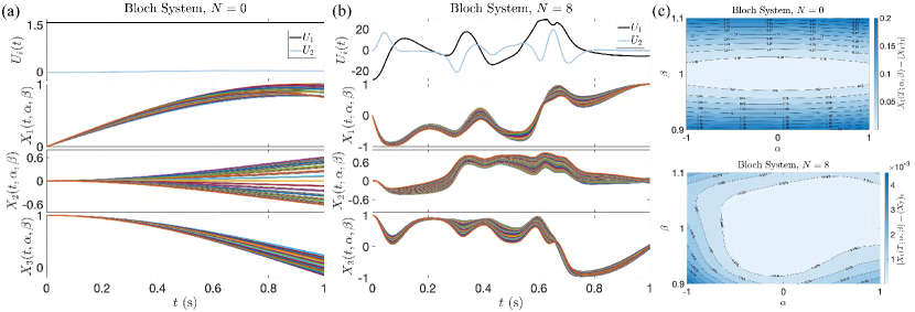
Figure 1: State transfer for the Bloch system with two different values of the maximum degree $N$ of the Legendre polynomials in equation (11). The control and state variables are shown for (a) $N=0$ and (b) $N=8$. (c) Error resulting over the parameter regions for $N=0$ (top) and $N=8$ (bottom).

The performance of the iterative quadratic programming algorithm presented in Section IV to solve the OCP described in Section II-B will be demonstrated for two examples that arise in quantum control applications. The computations are performed in Matlab R2023a on a MacBook Pro with 32 GB of usable memory and an Apple M2 Max processing chip. The quadratic program at each stage of the iteration is implemented with the general-purpose Matlab function quadprog using the sparse-linear-convex algorithm and sparse linear algebra operations. The CPU user load ranges between 12% and 60% of the maximum capability of the computer and the used memory is less than 3.5 GB.

V-A Nuclear Magnetic Resonance Spectroscopy

Imaging modalities that take advantage of nuclear magnetic resonance (NMR) apply a strong constant magnetic field to a sample of nuclei and then apply radio-frequency (RF) fields in the transverse plane to manipulate the nuclear spins of the sample. The spin dynamics are modeled using the Bloch equations [20, 25, 6]. The system of Bloch equations in a rotating reference frame without relaxation [26, 6] may be written as

$$\dot{X}=\begin{bmatrix}0&-\alpha&\beta U_{1}\\ \alpha&0&-\beta U_{2}\\ -\beta U_{1}&\beta U_{2}&0\end{bmatrix}X,$$ (31)

where $X(t;\alpha,\beta)$ represents the bulk magnetization of the nuclei, and $U_{1}(t)$ and $U_{2}(t)$ represent the applied field. Variations in system parameters appear as dispersion in the intrinsic frequencies of the nuclei and the strength of the applied field [27]. Here, the ensemble is defined by the continuum of parameter values $\alpha\in[-1,1]$ and $\beta\in[0.9,1.1]$, which respectively represent variations in Larmor frequency and the amplitude of the applied field. We seek controls $U_{1}(t)$ and $U_{2}(t)$ of minimal energy that steer the ensemble state from the zero-input equilibrium state $X_{0}=[0,0,1]^{\prime}$ to the excited state $X_{T}=[1,0,0]^{\prime}$. This example has received significant attention [9, 10, 13]. The example presented here demonstrates that the performance of our control approach is comparable to earlier contributions.

As previously shown [9, 13], the required degree $N$ of the truncated Legendre polynomial expansion generally increases as the specified terminal error tolerance $\epsilon$ in equation (5) is decreased. We analyze the effect of the performance for two different values of $N$. For the case $N=0$, the bilinear system of coefficients in equation (13) reduces to

$$\dot{x}(t)=\overline{\alpha}\mathcal{A}x(t)+\overline{\beta}\sum_{i=1}^{m}U_{i}(t)\mathcal{B}_{i}x(t),$$ (32)

with initial and terminal conditions $x(0)=2X_{0}$ and $\|x(T)-2X_{T}\|\leq\epsilon$. This system is equivalent to an individual system from the ensemble in equation (1) when sampled at the mean values $\alpha=\overline{\alpha}$ and $\beta=\overline{\beta}$. In this case, the aim of the control design is to find a minimal energy control action that steers only the nominal ensemble system. Therefore, one should expect the performance of this specific control action to be poor for parameter values far from the nominal values.

Figure 1 illustrates the control actions, state vectors, and error contour plots over the region of parameters for both $N=0$ and $N=8$. In addition to the parameters above, we use $T=1$ s, $K=500$, $U_{\min}=-30$, $U_{\max}=30$, $\lambda_{0}=0.1$, $\mu_{0}=20$, $\epsilon=0.001$, and $\delta=0.001$. The algorithm is initialized with the nominal control action $\overline{U}_{i}(t)=0$. We first discuss results with $N=0$. The total number of equations in (18) is $n(N+1)^{2}K=1500$ and the size of $H$ in equation (27) is $n(N+1)^{2}\times m(K-1)=3\times 998$. The algorithm converges to a minimum energy control after five iterations in less than five seconds. For $N=8$, the total number of equations in (18) is $121500$ and the size of $H$ in equation (27) is $243\times 998$. The algorithm converges after 643 iterations and the elapsed time is about 14 minutes. It is clear from Figure 1 that the control corresponding to $N=0$ results in poor performance compared to the control corresponding to $N=8$. In particular, the error contour plot shows that the error for $N=0$ is generally two orders of magnitude larger than the error for $N=8$. This verifies that a minimum energy control action computed with an individual sample of the bilinear ensemble system is generally not robust to parameter variation, and the polynomial moment approach successfully compensates for such variation.

V-B Ultra-Cold Atom Interferometry

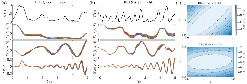
Figure 2: Control and state variables for splitting a BEC into (a) the $\pm 2\hbar k$ momentum level and (b) the $\pm 4\hbar k$ level. (c) Error resulting over the parameter regions for $\pm 2\hbar k$ (top) and $\pm 4\hbar k$ (bottom).

We consider a quantum control setting related to a proposed technique for interferometry, in which a dilute Bose-Einstein condensate (BEC) composed of atoms that are initially at rest is manipulated to elicit a diffraction pattern. The relevant dynamics for the initial matter-wave splitting are modeled using the Raman-Nath equations [28]. Standing-wave optical pulses modulated by square-shaped [29], Guassian [30], and other transcendental envelopes [31] were designed to split the stationary condensate into a definite state of high-order momentum or a superposition of such states. Recently, optimal control was applied to a bilinear ensemble that approximates the Raman-Nath equations with uncertainty in the intensity of the applied optical pulse [14]. There, the authors numerically demonstrate the ability to split the BEC into a high-order momentum state with a high degree of fidelity. In the current example, we extend the recent results to incorporate uncertainty in both light intensity and photon recoil energy [32].

The dynamics of the BEC may be described by a single wave function because the particles are indistinguishable and collectively occupy the same energy state. The wave function $\Psi(t,x)$ is governed by the one-dimensional Schrödinger equation [28, 31, 14],

$$i\frac{\partial\Psi}{\partial t}=-\frac{\hbar}{2m}\frac{\partial^{2}\Psi}{\partial x^{2}}+U(t)\cos^{2}(2k_{0}x)\Psi,$$ (33)

where $U(t)$ is the amplitude of the light shift potential and $k_{0}$ is the vacuum wave number of the photons. In this example, we adhere to convention and use the symbols $i$, $m$, and $x$ to denote the imaginary unit, the mass of the BEC, and the independent spatial variable, respectively. As in prior studies [28, 31], we make the following assumptions and expand $\Psi$ into a superposition of the zero momentum state with coefficient $C_{0}(t,k)$ and high-order symmetric and anti-symmetric momentum states with coefficients $C^{+}_{2n^{\prime}}(t,k)$ and $C^{-}_{2n^{\prime}}(t,k)$, where $k$ represents the wave number distribution of the manipulated atom. First, the wave function is initially in the zero momentum state. Second, there exists a positive integer $N^{\prime}$ such that $U(t)/2\ll(2N^{\prime})^{2}\omega_{r}$ for all $t\in[0,T]$, where $\omega_{r}=\hbar k_{0}^{2}/(2m)$ is the photon recoil energy. Third, the duration $T$ of the optical pulse is sufficiently short so that $k\ll k_{0}$ and the Raman-Nath approximation can be applied [32]. Then, as described in recent studies [14, 31], the dynamics of diffraction may be approximated by the reduced vector $\mathcal{X}=[C_{0},C_{2}^{+},\dots,C_{2N^{\prime}}^{+}]^{\prime}$ governed by

$$\dot{\mathcal{X}}=-i\left(\alpha\mathcal{A}_{0}+U(t)\beta\mathcal{B}_{0}\right)\mathcal{X},$$ (34)

where the $(N^{\prime}+1)\times(N^{\prime}+1)$ matrices are defined by $\mathcal{A}_{0}=\omega_{r}\text{diag}(0,4,\dots,(2N^{\prime})^{2})$ and

$$\mathcal{B}_{0}=\frac{1}{2}\begin{bmatrix}0&\sqrt{2}&&\\ \sqrt{2}&0&1&\\ &1&\ddots&1\\ &&1&0\end{bmatrix}.$$ (35)

We have integrated the parameters $\alpha\in[0.99,1.01]$ and $\beta\in[0.95,1.05]$ into the model to account for uncertainty in photon recoil energy and optical intensity, respectively. Finally, we expand the complex-valued state vector into its real and imaginary components and substitute the expression $\mathcal{X}=\text{Re}(\mathcal{X})+i\text{Im}(\mathcal{X})$ into equation (34). By equating real and imaginary parts and defining $X=[\text{Re}(\mathcal{X})^{\prime},\text{Im}(\mathcal{X})^{\prime}]^{\prime}$, the equivalent real-valued bilinear ensemble system is

$$\dot{X}(t)=\alpha\begin{bmatrix}0&\mathcal{A}_{0}\\ -\mathcal{A}_{0}&0\end{bmatrix}X(t)+U(t)\beta\begin{bmatrix}0&\mathcal{B}_{0}\\ -\mathcal{B}_{0}&0\end{bmatrix}X(t).$$

The initial and desired target states are defined by $X_{0}=[1,0,\dots,0]^{\prime}$ and $X_{T}=[0,\dots,0,1,0,\dots,0]^{\prime}$, where the only nonzero component of the target state appears in the $(n^{\prime}+1)$-th entry. Here, $n^{\prime}$ is an integer representative of the target momentum state $\pm 2n^{\prime}\hbar k$.

Figure 2 shows the control actions, state vectors, and error contour plots over the region of parameters for both $n^{\prime}=1$ and $n^{\prime}=2$. The BEC system is truncated at $N^{\prime}=4$, so that the dimension of the ensemble state vector $X(t,\alpha,\beta)$ is $n=10$. The other parameters used for the computation are $N=10$, $T=5$ s, $K=1000$, $U_{\min}=0$, $U_{\max}=30$, $\lambda_{0}=10$, $\mu_{0}=50$, $\epsilon=0.001$, and $\delta=0.008$. The algorithm is initialized with the nominal control action $\overline{U}(t)=1$. For both splitting examples, the total number of equations in (18) is $n(N+1)^{2}K=1210000$ and the size of $H$ in equation (27) is $n(N+1)^{2}\times m(K-1)=1210\times 999$. For $n^{\prime}=1$, the algorithm converges to a minimal energy control after 177 iterations in 45 minutes. For $n^{\prime}=2$, the algorithm converges after 223 iterations within 75 minutes. Figure 2 demonstrates that the control action is robust over the region of parameter values, but the fidelity is limited to two decimal digits. For the Bloch system example, $N=8$ polynomials is sufficient to achieve three decimal digit fidelity over the parameter space. We see that $N=10$ is generally insufficient for the BEC splitting system to achieve comparable performance. In order to improve fidelity, it may be necessary to double or even triple the values of $N$ and $K$. If these two parameters double in value, then the number of constraints in equation (18) exceed eight million. If these values are tripled, then the number of constraints in equation (18) exceed 28 million.

VI Conclusion

We have designed a computational method for open-loop minimum-norm control synthesis for fixed-endpoint transfer of bilinear ensemble systems that are indexed by two continuously varying parameters. The ensemble state is approximated using a truncated basis of Legendre polynomials. The dynamics are linearized at each stage of the iteration about control and state trajectories to formulate a sequence of quadratic programs for computing perturbations to the control that successively improve the objective until convergence. We show that the approximation quality depends on the order in which linearization and exact discretization are performed. In particular, we prove that the two orders of operations result in different systems that are approximately equivalent in the sense of numerical quadrature.

The developed two-stage interative quadratic programming algorithm for solving the formulated class of optimal control problems is demonstrated for the Bloch system that appears in nuclear magnetic resonance, as well as the Raman-Nath equations that appear in the matter-wave splitting step of ultra-cold atom interferometry. For the Bloch system, our algorithm robustly achieves uniform state transfer with a precision of up to three decimal places. The larger and more complex Raman-Nath system requires significantly larger values for the number of polynomials in the truncated approximation and the number of time steps in the numerical discretization scheme. As mentioned above, pulse design for the Raman-Nath system can result in over 20 million constraints for the discrete-time linear system at each state of the iteration. Although the computation of trajectories and linear system approximations are performed without symbolic algebra, the matrices and time evolution are currently updated with a for-loop at each stage of the iteration. This is generally not scalable in Matlab to systems with tens of millions of constraints. Future work can extend the iterative quadratic programming approach presented here to more computationally expedient and tractable formulations that involve purely matrix-vector operations, and may benefit from the use of high performance computing.

References

- [1] Zijad Aganovic and Zoran Gajic. The successive approximation procedure for finite-time optimal control of bilinear systems. IEEE Transactions on Automatic Control, 39(9):1932–1935, 1994.
- [2] E. P. Hofer and B. Tibken. An iterative method for the finite-time bilinear-quadratic control problem. Journal of Optimization Theory and Applications, 57:411–427, 1988.
- [3] Shuo Wang and Jr-Shin Li. Fixed-endpoint optimal control of bilinear ensemble systems. SIAM Journal on Control and Optimization, 55(5):3039–3065, 2017.
- [4] Karine Beauchard, Jean-Michel Coron, and Pierre Rouchon. Controllability issues for continuous-spectrum systems and ensemble controllability of Bloch equations. Communications in Mathematical Physics, 296(2):525–557, 2010.
- [5] Wei Zhang and Jr-Shin Li. Analyzing controllability of bilinear systems on symmetric groups: Mapping Lie brackets to permutations. IEEE Transactions on Automatic Control, 65(11):4895–4901, 2019.
- [6] Jr-Shin Li and Navin Khaneja. Ensemble control of Bloch equations. IEEE Transactions on Automatic Control, 54(3):528–536, 2009.
- [7] Jr-Shin Li, Wei Zhang, and Lin Tie. On separating points for ensemble controllability. SIAM Journal on Control and Optimization, 58(5):2740–2764, 2020.
- [8] Xing Wang, Bo Li, Jr-Shin Li, Ian R. Petersen, and Guodong Shi. Controllability and accessibility on graphs for bilinear systems over Lie groups. IEEE Trans. Automatic Control, 68(4):2277–2292, 2023.
- [9] Jr-Shin Li, Justin Ruths, Tsyr-Yan Yu, Haribabu Arthanari, and Gerhard Wagner. Optimal pulse design in quantum control: A unified computational method. Proceedings of the National Academy of Sciences, 108(5):1879–1884, 2011.
- [10] Anatoly Zlotnik and Shin Li. Iterative ensemble control synthesis for bilinear systems. In 2012 IEEE 51st IEEE Conference on Decision and Control (CDC), pages 3484–3489. IEEE, 2012.
- [11] Justin Ruths and Jr-Shin Li. A multidimensional pseudospectral method for optimal control of quantum ensembles. The Journal of Chemical Physics, 134(4), 2011.
- [12] Vignesh Narayanan, Wei Zhang, and Jr-Shin Li. Moment-based ensemble control. arXiv preprint arXiv:2009.02646, 2020.
- [13] Xin Ning, Andre Luiz P De Lima, and Jr-Shin Li. NMR pulse design using moment dynamical systems. In 61st Conference on Decision and Control (CDC), pages 5167–5172. IEEE, 2022.
- [14] Andre Luiz P. de Lima, Andrew K. Harter, Michael J. Martin, and Anatoly Zlotnik. Optimal ensemble control of matter-wave splitting in Bose-Einstein condensates. arXiv preprint arXiv:2309.08807, 2023.
- [15] Minh Vu and Shen Zeng. Iterative optimal control syntheses for nonlinear systems in constrained environments. In 2020 American control conference (ACC), pages 1731–1736. IEEE, 2020.
- [16] Claudio Altafini and Francesco Ticozzi. Modeling and control of quantum systems: An introduction. IEEE Transactions on Automatic Control, 57(8):1898–1917, 2012.
- [17] Aaron Becker and Timothy Bretl. Approximate steering of a plate-ball system under bounded model perturbation using ensemble control. In 2012 IEEE/RSJ International Conference on Intelligent Robots and Systems, pages 5353–5359. IEEE, 2012.
- [18] Laurence Grammont, Mario Ahues, and Filomena D. d’Almeida. For nonlinear infinite dimensional equations, which to begin with: linearization or discretization? The Journal of Integral Equations and Applications, 26(3):413–436, 2014.
- [19] Dimitri Breda, Odo Diekmann, Mats Gyllenberg, Francesca Scarabel, and Rossana Vermiglio. Pseudospectral discretization of nonlinear delay equations: new prospects for numerical bifurcation analysis. SIAM Journal on applied dynamical systems, 15(1):1–23, 2016.
- [20] John Pauly, Patrick Le Roux, Dwight Nishimura, and Albert Macovski. Parameter relations for the shinnar-le roux selective excitation pulse design algorithm (nmr imaging). IEEE Transactions on Medical Imaging, 10(1):53–65, 1991.
- [21] Shen Zeng and Frank Allgoewer. A moment-based approach to ensemble controllability of linear systems. Systems & Control Letters, 98:49–56, 2016.
- [22] Uri M. Ascher and Chen Greif. A first course on numerical methods. SIAM, 2011.
- [23] T. M. Apostol. Calculus: Multi-variable calculus and linear algebra, with applications to differential equations and probability. Wiley, 1967
- [24] Minh Vu and Shen Zeng. An iterative online approach to safe learning in unknown constrained environments. In 2023 62nd IEEE Conference on Decision and Control (CDC), pages 7330–7335. IEEE, 2023.
- [25] Hideo Mabuchi and Navin Khaneja. Principles and applications of control in quantum systems. International Journal of Robust and Nonlinear Control: IFAC-Affiliated Journal, 15(15):647–667, 2005.
- [26] Henry C. Torrey. Bloch equations with diffusion terms. Physical Review, 104(3):563, 1956.
- [27] Malcolm H. Levitt. Composite pulses. Progress in Nuclear Magnetic Resonance Spectroscopy, 18(2):61–122, 1986.
- [28] Saijun Wu, Ying-Ju Wang, Quentin Diot, and Mara Prentiss. Splitting matter waves using an optimized standing-wave light-pulse sequence. Physical Review A, 71(4):043602, 2005.
- [29] Mark Edwards, Brandon Benton, Jeffrey Heward, and Charles W. Clark. Momentum-space engineering of gaseous Bose-Einstein condensates. Physical Review A, 82(6):063613, 2010.
- [30] Holger Müller, Sheng-wey Chiow, and Steven Chu. Atom-wave diffraction between the Raman-Nath and the Bragg regime: Effective Rabi frequency, losses, and phase shifts. Physical Review A, 77(2):023609, 2008.
- [31] Mary Clare Cassidy, Malcolm G. Boshier, and Lee E. Harrell. Improved optical standing-wave beam splitters for dilute Bose–Einstein condensates. Journal of Applied Physics, 130(19), 2021.
- [32] Gretchen K. Campbell et al. Photon recoil momentum in dispersive media. Physical Review Letters, 94(17):170403, 2005.