Competition between allowed and first-forbidden $\beta$ decay in $r$-process waiting-point nuclei within a relativistic beyond-mean-field approach

Abstract

Background

$\beta$-decay rates of neutron-rich nuclei are a crucial ingredient to the simulations of the $r$-process nucleosynthesis. Up to now global calculations of these rates have been performed within the quasiparticle random-phase approximation (QRPA) which is known to have limited accuracy and predictive power due to a limited treatment of nuclear correlations. Although extensions of this approach have been developed to include a more precise description of correlations, and have been applied to the study of allowed $\beta$-decay of selected nuclei, no systematic calculations including first-forbidden transitions have so far been performed.

Purpose

The goal of this work is to compute $\beta$-decay half-lives of isotonic nuclear chains located at neutron shell closures $N=50$, $82$, $126$ and $184$, which are of particular importance for the $r$-process nucleosynthesis, and study the role of first-forbidden transitions in a framework that includes complex nucleonic correlations beyond the QRPA.

Method

The many-body approach based on the relativistic QRPA extended to account for the coupling between single-particle and collective degrees of freedom is applied. Both Gamow-Teller and first-forbidden contributions to the decay rates are considered

Results

Overall, the fragmentation of the transition strength distributions due to the coupling between single particles and collective vibrations systematically increases the transition strength at low excitation energies and yields a decrease of the $\beta$-decay half-lives which is particularly important for low Q-values. Such effects are crucial to bring Gamow-Teller transitions within the decay energy window, and to reproduce the measured decay rates. Generally, quasiparticle-vibration coupling tends to decrease the probability of decay via FF transition near stability, due to the appearance of Gamow-Teller transitions within the decay $Q$ value. While in the lighter systems allowed transitions dominate, the decay of $N=126$ and $N=184$ nuclei is found to occur to a large extent via first-forbidden transitions, and in particular those induced by $1^{-}$ and $0^{-}$ operators.

Conclusions

The relativistic approach based on the coupling between nucleons and vibrations has the ability to capture relevant correlations that are essential for an accurate predictions of $\beta$-decay and provides an ideal framework for future large-scale calculations. Upcoming experimental measurements of $\beta$-decay rates in the $N=126$ region by radioactive-beam facilities will be crucial in order to validate the approach.

I Introduction

The synthesis of heavy elements via the $r$ process [1, 2] is an extremely complex phenomenon which involves several thousands of nuclei and a delicate interplay between various reaction and decay mechanisms such as neutron capture, $\beta^{-}$ decay and fission. Although the multi-messenger neutron star merger event GW170817 [3] has provided tremendous information, a full comprehension of the $r$-process nucleosynthesis requires a more precise understanding of the nuclear physics involved. In particular, an accurate knowledge of masses, $\beta$-decay half-lives, neutron-capture rates and fission yields, to name a few, are needed [4, 5, 6, 7, 8]. Out of these many ingredients, $\beta$-decay half-lives are of great importance as they set the time scale of the nucleosynthesis and also have a crucial impact on the final abundance pattern [9, 10, 11, 6, 12, 13]. Because most of the nuclei of interest to the $r$ process are extremely short lived, they cannot be produced in laboratories and thus, astrophysical simulations heavily rely on theoretical predictions. Providing consistent, precise and predictive nuclear physics input, for the whole range of nuclei involved, is a tremendous challenge for nuclear theory. Microscopic methods based on the self-consistent mean field or density functional theory (DFT) in principle represent good candidates to reach this goal as they can provide a consistent description of most of the nuclear chart. However, in their present forms, most of these approaches suffer important limitations and do not meet the degree of precision needed for reliable astrophysical simulations.

The method currently used to provide global sets of $\beta$-decay rates is known as the quasiparticle random phase approximation (QRPA) [14], applied in the charge-exchange (proton-neutron) channel, and corresponds to the small amplitude limit of the time-dependent mean field or time-dependent DFT. Several relativistic and non-relativistic versions have been developed and applied to the calculations of $\beta^{-}$ decay (see e.g. Refs. [15, 16, 17, 18, 19, 20, 21, 22, 23, 13, 24]). Overall it is known that QRPA suffers from major shortcomings as it only includes a very limited amount of correlations in the description of nuclei due to the neglect of retardation effects in the one-nucleon self-energy. In the charge-exchange channel, this basically restricts the daughter configurations to one-particle-one-hole (1p-1h), or two-quasiparticle (2qp), proton-neutron excitations of the parent ground state. Such approximation typically leads to an imprecise description of transition strength distributions, in particular the very low-energy states, that are essential for an accurate prediction of decay rates. To compensate, QRPA usually relies on extra empirical parameters (proton-neutron pairing) which have to be fitted to the $\beta$-decay half-lives, sometimes separately for each mass region [15, 18]. Such a procedure drastically limits the reliability and predictive power of this approach, in particular in unexplored regions of the nuclear chart. As of today, the three existing global sets of $\beta$-decay rates have been calculated within different versions of the charge-exchange QRPA. The earlier set is based on the finite range droplet model (FRDM) and combines a microscopic description of Gamow-Teller (GT) transitions using a schematic separable interaction with a description of the first-forbidden (FF) modes based on the gross theory [17]. More recently, two self-consistent and fully microscopic QRPA calculations have become available: Ref. [13] based on a covariant framework and Ref. [24] based on a non-relativistic Skyrme functional. While the former allowed a fully relativistic treatment of $\beta$-decay operators, it considered all nuclei as spherical and treated odd systems in the same way as paired even-even nuclei with an odd number of nucleons on average. The latter, on the other hand, relied on non-relativistic reductions of the transition operators but incorporated a more correct treatment of deformation and odd systems. Overall, the predictions of these three QRPA frameworks disagree on several points, in particular on the relative importance of GT and FF transitions in different mass regions and on the order of magnitude of the total rates above $N=126$. These discrepancies constitute an important problem as they can lead to large uncertainties in subsequent astrophysical simulations and predictions of elemental abundances [12]. For example, it was found in Refs. [13, 6] that the shortenings of half-lives in the heavy region yields a broadening of the third $r$-process abundance peak towards lower masses.

While understanding the origin of the discrepancies between the QRPA predictions constitute an interesting problem on its own and should be investigated further, in order to ultimately limit the uncertainties of $r$-process simulations related to the nuclear physics input, it is desirable to develop extensions of the (Q)RPA to incorporate higher-order dynamical processes in the nucleonic self-energy and a more precise treatment of correlations in the nuclear response. Such approaches include the Second RPA (SRPA) and methods based on the coupling of single nucleons to collective nuclear vibrations (phonons). SRPA introduces a second-order treatment of the nucleonic self-energy leading to explicit 2p-2h configurations in the excited states. Recently a charge-exchange version of this approach based on a Skyrme functional was applied to GT transitions and $\beta^{-}$-decay of a few nuclei [25, 26]. However, due to the large number of 2p-2h configurations, and because the available versions are currently limited to doubly magic nuclei, the present range of applicability of this approach remains limited. On the other hand, methods based on the particle-vibration coupling (PVC), and its extension to open-shell nuclei —quasiparticle vibration-coupling (QVC)— provide an efficient and relatively low-cost way to include complex nucleonic configurations relevant to mid- and heavy-mass nuclei. In this approach, virtual particle-hole excitations are included up to infinite order in the nucleonic self-energy and excitations are built from 1p-1h $\otimes$ phonon configurations on top of the initial state. Microscopic versions of the PVC scheme include the non-relativistic one based on Skyrme interactions [27] as well as the relativistic framework based on the meson-nucleon Lagrangian [28]. These two frameworks have been successfully applied to GT and $\beta$ decay of selected closed and open-shell nuclei [29, 30, 31, 32, 33, 34, 35, 36]. Recently, the formalism of QVC based on a Skyrme functional has been successively extended and applied to the description of GT modes and $\beta$-decay of a few deformed nuclei within the finite amplitude method [37]. Overall the coupling of nucleons to vibrations induces fragmentation and spreading of the transition strength distribution which have been found crucial for an accurate description of the width of the Gamow-Teller resonances and $\beta$-decay half-lives. So far, however, no extensive study of $\beta$ decay including FF transitions have been performed, even though these transitions are known to importantly contribute to the decay in many nuclei relevant to the $r$ process, due to large neutron excess.

Although global calculations are not presently possible, one can study selected regions along the $r$-process path. Among those, the so-called waiting-point nuclei, located at neutron shell closures, are of crucial importance. Because these nuclei present low $Q$-values for neutron capture, a long sequence of alternating $\beta$ decay and neutron capture takes place until the $r$-process can move to heavier neutron numbers. Matter thus accumulates at nuclei closer to stability with long beta-decay half-lives and leads to peaks in the abundance patterns. While experimental measurements of neutron-rich $N=50$ and $N=82$ nuclei have been performed, almost no data is available yet for the $N=126$ and $N=184$ chains (see e.g. Ref. [4] for a recent review on the experimental status). The $N=126$ isotones are particularly interesting because they have been calculated within several theoretical frameworks which largely disagree on the contribution of the forbidden transitions [17, 16, 21, 13, 24, 38, 39].

In the present work, we perform systematic calculations of $\beta^{-}$-decay half-lives of even-even nuclei with magic neutron numbers $N=50,82,126$ and $184$ within the relativistic QVC framework and include both allowed GT and FF transitions. The manuscript is organized as follows. In section II we review the formalism of our approach. We present both the theory of $\beta^{-}$-decay that we apply and the formalism of our nuclear many-body method. The numerical scheme is also explained in detail. In section III we present the $\beta^{-}$-decay half-lives of the $r$-process waiting-point nuclei and study the role of QVC and its interplay with first-forbidden transitions. In section IV we compare our results to other existing theoretical calculations.

II Formalism

II.1 Theory of allowed and first-forbidden $\beta$-decay

In this work we follow the theory of allowed and forbidden $\beta$-decay as was derived by Behrens and Buehring [40]. The equations have already been summarized in a number of papers, as for instance Ref. [13]. Below we repeat them for completeness.

The rate $\lambda_{\text{tot}}$ for the $\beta^{-}$ decay from a parent nucleus $(Z,N)$, initially in its ground state, to states in the daughter nucleus $(Z+1,N-1)$ reads

$$\lambda_{\text{tot}}=\frac{\mbox{ln 2}}{K}\sum_{f,E_{f}<m_{e}}\Psi(E_{f},Z+1)\;.$$ (1)

In Eq. 1, $K=6144\pm 2$ s [41], the index $f$ denotes the states of the daughter nucleus, $E_{f}$ is the decay energy of these states defined as $E_{f}=M_{f}-M_{i}$, where $M_{i}$ and $M_{f}$ are the initial and final nuclear masses, respectively. The summation is restricted to states that are energetically accessible (with energy $E_{f}$ up to the electron mass $m_{e}$). Finally, $\Psi(E_{f},Z+1)$ is the so-called integrated shape function. When both allowed and FF transitions are considered, this function takes the form

$$\Psi(E_{f},Z+1)= \int_{1}^{W_{f}}dWW\sqrt{W^{2}-1}(W_{f}-W)^{2}$$

$$\times F(Z+1,W)C(W)\;.$$

In Eq. LABEL:eq:shape_fct, $W=E_{e}/m_{e}$ denotes the electron energy in unit of the electron mass, $W_{f}\equiv(M_{i}-M_{f})/m_{e}=-(E_{f}/m_{e})$ is the maximal electron energy, and $F(Z+1,W)$ is the Fermi function [40] accounting for the Coulomb interaction between the emitted electron and the daughter nucleus. Finally, $C(W)=C_{\text{all.}}(W)$ or $C_{\text{FF}}(W)$ is the shape factor corresponding to the allowed or FF transition, as described below.

In the case of allowed transitions, the shape factor $C_{\text{all.}}(W)$ is in fact independent of the energy $W$ and coincides with the GT reduced transition probabilities,

$$C_{\text{all.}}=B(\text{GT})=g_{A}^{2}\frac{|\langle f||\bm{O}_{GT}||i\rangle|^{2}}{2J_{i}+1}\;,$$ (3)

where $g_{A}=-1.2764(13)$ [42] is the weak axial coupling constant, $J_{i}$ is the angular momentum of the initial state, and $\bm{O}_{GT}$ is the relativistic GT transition operator

$$\bm{O}_{GT}=\sum_{k=1}^{A}\bm{\Sigma}^{k}\,\bm{t}_{-}^{k}=\sum_{k=1}^{A}\begin{pmatrix}\bm{\sigma}^{k}&0\\ 0&\bm{\sigma}^{k}\end{pmatrix}\bm{t}_{-}^{k}\;,$$ (4)

with $\bm{\sigma}$ the Pauli spin operator and $\bm{t}_{-}=\bm{\tau}/2$ the operator converting a neutron into a proton.

In the case of first-forbidden decays, the shape factor $C_{\text{FF}}(W)$ depends on the energy $W$ and the nuclear transition matrix elements of forbidden operators:

$$C_{\text{FF}}(W)=k+ka\,W+kb\,W^{-1}+kc\,W^{2}\;.$$ (5)

Within the formalism of Behrens and Buehring [40], the coefficients $k$, $ka$, $kb$ and $kc$ read

$$k = \bigl{[}\zeta_{0}^{2}+\frac{1}{9}w^{2}\bigr{]}_{(0)}$$ (6)

$$+\bigl{[}\zeta_{1}^{2}+\frac{1}{9}(x+u)^{2}-\frac{4}{9}\mu_{1}\gamma_{1}u(x+u)$$

$$+\frac{1}{18}W_{f}^{2}(2x+u)^{2}-\frac{1}{18}\lambda_{2}(2x-u)^{2}\bigl{]}_{(1)}$$

$$+\bigl{[}\frac{1}{12}z^{2}(W_{f}^{2}-\lambda_{2})\bigr{]}_{(2)}\;,$$

$$ka = \bigl{[}-\frac{4}{3}uY-\frac{1}{9}W_{f}(4x^{2}+5u^{2})\bigr{]}_{(1)}$$ (7)

$$-\bigl{[}\frac{1}{6}W_{f}z^{2}\bigr{]}_{(2)}\;,$$

$$kb = \frac{2}{3}\mu_{1}\gamma_{1}\left(-\bigl{[}\zeta_{0}w\bigr{]}_{(0)}+\bigl{[}\zeta_{1}(x+u)\bigr{]}_{(1)}\right)\;,$$ (8)

$$kc = \frac{1}{18}\bigl{[}8u^{2}+(2x+u)^{2}+\lambda_{2}(2x-u)^{2}\bigr{]}_{(1)}$$ (9)

$$+\frac{1}{12}\bigl{[}(1+\lambda_{2})z^{2}\bigr{]}_{(2)}\;,$$

where

$$\zeta_{0} =V+\frac{1}{3}wW_{f} \mbox{ with }V=\xi^{\prime}v+\xi w^{\prime}$$ (10)

$$\zeta_{1} =Y+\frac{1}{3}(u-x)W_{f} \mbox{ with }Y=\xi^{\prime}y-\xi(u^{\prime}+x^{\prime})$$ (11)

$$\gamma_{1} =\sqrt{1-(\alpha Z)^{2}}\;.$$ (12)

In the above equations, $\xi=\alpha Z/2R$ where $\alpha$ is the fine structure constant and $R$ is the radius of a uniformly charged sphere approximating the nuclear charge distribution. Under this approximation, $R$ is determined from the root mean square charge radius $\sqrt{\langle r\rangle^{2}}$ (calculated in the mean-field approximation, see section II.3) as $R=\sqrt{5\langle r\rangle^{2}/3}$. The parameters $\mu_{1}$ and $\lambda_{2}$ are related to the emitted electron and are approximated by $\mu_{1}=1$ and $\lambda_{2}=1$ [43, 44]. The number $(J)$ in subscript after the square brackets in Eqs. (6)-(9) denotes the rank of the operators appearing in the bracket.

The nuclear transition matrix elements are given by (in the Condon-Shortley phase convention)

$$w=-g_{A}\sqrt{3}\hat{J}_{i}^{-1}\langle f||\sum_{k}r_{k}\bigl{[}\bm{C}_{1}^{k}\otimes\bm{\Sigma}^{k}\bigr{]}_{(0)}\bm{t}_{-}^{k}||i\rangle\;,$$ (13)

$$x=-\hat{J}_{i}^{-1}\langle f||\sum_{k}r_{k}\bm{C}_{1}^{k}\bm{t}_{-}^{k}||i\rangle\;,$$ (14)

$$u=-g_{A}\sqrt{2}\hat{J}_{i}^{-1}\langle f||\sum_{k}r_{k}\bigl{[}\bm{C}_{1}^{k}\otimes\bm{\Sigma}^{k}\bigr{]}_{(1)}\bm{t}_{-}^{k}||i\rangle\;,$$ (15)

$$z=2g_{A}\hat{J}_{i}^{-1}\langle f||\sum_{k}r_{k}\bigl{[}\bm{C}_{1}^{k}\otimes\bm{\Sigma}^{k}\bigr{]}_{(2)}\bm{t}_{-}^{k}||i\rangle\;,$$ (16)

$$w^{\prime}=-g_{A}\frac{2}{\sqrt{3}}\hat{J}_{i}^{-1}$$

$$\hskip 5.69054pt\times\langle f||\sum_{k}r_{k}I(1,1,1,1,r_{k})\bigl{[}\bm{C}_{1}^{k}\otimes\bm{\Sigma}^{k}\bigr{]}_{(0)}\bm{t}_{-}^{k}||i\rangle\;,$$ (17)

$$x^{\prime}=-\frac{2}{3}\hat{J}_{i}^{-1}$$

$$\hskip 5.69054pt\times\langle f||\sum_{k}r_{k}I(1,1,1,1,r_{k})\bm{C}_{1}^{k}\bm{t}_{-}^{k}||i\rangle\;,$$ (18)

$$u^{\prime}=-g_{A}\frac{2\sqrt{2}}{3}\hat{J}_{i}^{-1}$$

$$\hskip 5.69054pt\times\langle f||\sum_{k}r_{k}I(1,1,1,1,r_{k})\bigl{[}\bm{C}_{1}^{k}\otimes\bm{\Sigma}^{k}\bigr{]}_{(1)}\bm{t}_{-}^{k}||i\rangle\;,$$ (19)

where

$$\bm{C}_{LM}=\sqrt{\frac{4\pi}{2L+1}}Y_{LM}\;,$$ (20)

and $\hat{J}_{i}\equiv\sqrt{2J_{i}+1}=1$ in the case of decay from even-even ground states. The function $I(1,1,1,1,r_{k})$ accounts for the nuclear charge distribution which is approximated by a uniform spherical charge distribution as [40]

$$I(1,1,1,1,r_{k})=\frac{3}{2}\left\{\begin{array}[]{ll}\displaystyle{1-\frac{1}{5}\left(\frac{r}{R}\right)^{2}\;,0\leq r\leq R\;,}\\[11.38109pt] \displaystyle{\frac{R}{r}-\frac{1}{5}\left(\frac{R}{r}\right)^{3}\;,r>R\;.}\end{array}\right.$$ (23)

Finally the transition matrix elements originating from relativistic contributions are

$$\xi^{\prime}v = -g_{A}\hat{J}_{i}^{-1}\langle f||\sum_{k}\gamma_{5}^{k}\bm{t}_{-}^{k}||i\rangle\;,$$ (24)

$$\xi^{\prime}y = -\hat{J}_{i}^{-1}\langle f||\sum_{k}\bm{\alpha}^{k}\bm{t}_{-}^{k}||i\rangle\;,$$ (25)

where $\bm{\alpha}=\gamma^{0}\bm{\gamma}$. These transitions connect the small and large components of the Dirac spinors, and thus, also change the parity of the nuclear state. Since we will work in a relativistic framework, we do not perform any non-relativistic reductions of the matrix elements (24) and (25).

II.2 Nuclear Many-Body Method: Proton-Neutron Relativistic Time Blocking Approximation (RQTBA)

In this work the nuclear transition matrix elements are calculated within the relativistic charge-exchange (or proton-neutron) QVC approach which represents an extension of the charge-exchange relativistic QRPA (RQRPA) accounting for the coupling between single quasiparticles and collective nuclear vibrations, as first developed in Ref. [33].

This approach is based on the calculation of the transition strength distribution $S({\bm{O}},E)$

$$S({\bm{O}},E) = \sum_{f}|\braket{f}{\bm{O}}{i}|^{2}\delta(E-E_{f})\,,$$ (26)

which characterizes the response of a nucleus to an external field $\bm{O}$. Here $\bm{O}$ will coincide with the GT or FF operators from section II.1, which convert neutrons into protons. In Eq. (26), $E$ denotes the energy variable, and as in the previous section, $\ket{i}$ and $\ket{f}$ are the initial parent ground state and final daughter state, respectively. The definition (26) for the strength distribution can easily be re-written in terms of the response function $R(\omega)$, or propagator of a correlated proton-neutron quasiparticle pair in the nuclear medium (see appendix A), as

$$S(\bm{O},E) = -\frac{1}{\pi}\lim_{\Delta\rightarrow 0^{+}}\mbox{Im}\sum_{1234}O_{12}^{*}R_{1423}(\omega)O_{34}\;,$$ (27)

where $\omega=E+i\Delta$ is the complex energy variable. In Eq. (27) we have introduced a single-quasiparticle basis $i=\{\eta_{i},k_{i}\}$ where $k_{i}=\{n_{i},\pi_{i},j_{i}\}$ denotes single-particle states and $\eta_{i}=\pm$ denotes the upper and lower component in the Nambu-Gorkov space, for nuclei with superfluid pairing correlations. In the following we will use odd (resp. even) numbers to denote proton (resp. neutron) single-particle states.

In the present framework, the response function is obtained within the framework of the linear response theory, by solving the following Bethe-Salpeter equation which accounts for QVC effects in the time-blocking approximation [45]:

$$R_{1423}(\omega) = \widetilde{R}^{(0)}_{1423}(\omega)$$

$$+\sum_{5678}\widetilde{R}^{(0)}_{1625}(\omega)W_{5867}(\omega)R_{7483}(\omega)\;.$$

The free two-quasiparticle proton-neutron propagator $\widetilde{R}^{(0)}$ is given by

$$R^{(0)}_{1423}(\omega)=\frac{\delta_{\eta_{1},-\eta_{2}}\delta_{\eta_{3},-\eta_{4}}\delta_{13}\delta_{24}}{\eta_{1}(\omega-\lambda_{pn})-\mathcal{E}_{k_{1}}-\mathcal{E}_{k_{2}}}\;,$$

where $\mathcal{E}_{k_{i}}$ and $\mathcal{E}_{k_{i}}$ are neutron and proton quasiparticle energies, respectively, and $\lambda_{pn}=\lambda_{p}-\lambda_{n}$ is the proton-neutron chemical potential difference.

The effective proton-neutron interaction $W(\omega)$ is given by

$$W(\omega)=\widetilde{V}+\Phi(\omega)\;,$$ (30)

which is the sum of the static interaction $\widetilde{V}$ and an energy-dependent term $\Phi(\omega)$ responsible for damping effects. The interaction $\Phi(\omega)$ originates from QVC and describes the virtual emission and re-absorption of a nuclear vibration by a quasiparticle, as well as the exchange of a vibration between a proton and a neutron quasiparticle, as represented in Fig. 1.

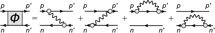
Figure 1: Energy-dependent proton-neutron QVC interaction $\Phi(\omega)_{pn^{\prime},np^{\prime}}$ from Eq. (LABEL:eq:Phi). The gray blobs represent the vertices of Eq. 32.

It is given by

$$\Phi_{1423}(\omega) \equiv \Phi^{\eta_{1}\eta_{4},\eta_{2}\eta_{3}}_{p_{1}n_{4},n_{2}p_{3}}(\omega)$$

$$= \delta_{\eta_{1},\eta_{3}}\delta_{\eta_{1},-\eta_{2}}\delta_{\eta_{3},-\eta_{4}}\times\sum_{\mu\xi}\delta_{\xi,\eta_{1}}$$

$$\times\Bigl{[} \delta_{k_{1}k_{3}}\sum_{k_{6}}\frac{g_{\mu;k_{6}k_{2}}^{\eta_{1};-\xi-\xi}g_{\mu;k_{6}k_{4}}^{\eta_{1};-\xi-\xi*}}{\eta_{1}(\omega-\lambda_{pn})-\mathcal{E}_{k_{1}}-\mathcal{E}_{k_{6}}-\Omega_{\mu}}$$

$$+\delta_{k_{2}k_{4}}\sum_{k_{5}}\frac{g_{\mu;k_{1}k_{5}}^{\eta_{1};\xi\xi}g_{\mu;k_{3}k_{5}}^{\eta_{1};\xi\xi*}}{\eta_{1}(\omega-\lambda_{pn})-\mathcal{E}_{k_{5}}-\mathcal{E}_{k_{2}}-\Omega_{\mu}}$$

$$-\frac{g_{\mu;k_{1}k_{3}}^{\eta_{1};\xi\xi}g_{\mu;k_{2}k_{4}}^{\eta_{1};-\xi-\xi*}}{\eta_{1}(\omega-\lambda_{pn})-\mathcal{E}_{k_{3}}-\mathcal{E}_{k_{2}}-\Omega_{\mu}}$$

$$-\frac{g_{\mu;k_{3}k_{1}}^{\eta_{1};\xi\xi*}g_{\mu;k_{4}k_{2}}^{\eta_{1};-\xi-\xi}}{\eta_{1}(\omega-\lambda_{pn})-\mathcal{E}_{k_{1}}-\mathcal{E}_{k_{4}}-\Omega_{\mu}}\Bigr{]}\;,$$

where the index $\mu$ labels the collective phonons of frequency $\Omega_{\mu}$ that couple to the quasiparticle states through the vertices

$$g_{\mu;k_{1}k_{2}}^{\eta_{\mu};\eta_{1}\eta_{2}}=\delta_{\eta_{\mu},+1}g_{\mu;k_{1}k_{2}}^{\;\eta_{1}\eta_{2}}+\delta_{\eta_{\mu},-1}g_{\mu;k_{2}k_{1}}^{\;\eta_{2}\eta_{1}*}\;,$$ (32)

where $k$ denotes generic nucleon states. These vertices are obtained from the solutions of the RQRPA as

$$g_{\mu;k_{1}k_{2}}^{\;\eta_{1}\eta_{2}}=\sum_{k_{3}k_{4}}\sum_{\eta_{3}\eta_{4}}\widetilde{V}_{k_{1}k_{4},k_{2}k_{3}}^{\eta_{1}\eta_{4}\eta_{2}\eta_{3}}\mathcal{R}_{\mu;k_{3}k_{4}}^{\;\eta_{3}\eta_{4}}\;,$$ (33)

where $\mathcal{R}_{\mu;k_{3}k_{4}}^{\;\eta_{3}\eta_{4}}$ denotes the RQRPA transition densities associated with each phonon $\mu$.

Due to the time-blocking approximation [45] that was applied in order to derive Eq. (LABEL:eq:BSE_pn) the approach described above has usually been referred to as proton-neutron Relativistic Quasiparticle Time Blocking Approximation (RQTBA) [33]. We will use this term throughout the paper. Note that when $\Phi(\omega)$ is neglected, Eq. (LABEL:eq:BSE_pn) reduces to the usual proton-neutron RQRPA.

II.3 Numerical scheme

The starting point of the present approach is the effective Lagrangian which describes the interaction between Dirac nucleons in terms of meson ($\pi$, $\sigma$, $\omega$ and $\rho$) and photon exchange. Because retardation effects are neglected, the resulting meson-exchange interaction $\widetilde{V}$ is static [46].

Relativistic mean field:

In order to determine the basis of quasiparticle states $(k_{i},\eta_{i})$, we start from a relativistic mean-field (RMF) calculation. In this work we consider the NL3 parametrization of the meson-nucleon Lagrangian [47], which includes non-linear $\sigma$ terms, and whose coupling constants were fitted to reproduce masses and radii of a few doubly-magic nuclei in the RMF approximation. This parametrization was found to give a good description of GT low-energy modes and giant resonances in previous studies [33, 34]. Since the RMF does not include the exchange interaction (Fock term), the pion does not contribute at this level (as it would break parity) [46] and thus, is not included in the NL3 Lagrangian.

In order to treat open-shell nuclei, we also include neutron-neutron and proton-proton isovector ($T=1$) pairing correlations. It is well known that in calculations based on the RMF, the pairing part of the interaction is usually treated on a different footing than the particle-hole (meson-exchange) component. Indeed, even though attempts were made to describe pairing correlations from the effective meson-exchange force, such studies so far did not succeed in reproducing the empirical pairing gaps [48, 49]. Thus typically one uses a different (non-relativistic) ansatz to describe the pairing component. In this work we use a simple monopole-monopole force for the $T=1$ pairing (particle-particle) channel [50]:

$$\widetilde{V}_{(k_{1}k_{2}k_{3}k_{4})}^{(\mathfrak{p}\mathfrak{p})(J,T=1)}= -\frac{G}{2}\delta_{J0}\delta_{(k_{1}k_{2})}\delta_{(k_{3}k_{4})}\sqrt{\frac{2j_{k_{1}}+1}{1+e^{(\varepsilon_{k_{1}}-w)/d}}}$$ (34)

$$\times\sqrt{\frac{2j_{k_{3}}+1}{1+e^{(\varepsilon_{k_{3}}-w)/d}}}\;,$$

for which the relativistic Hartree-Bogoliubov equations reduce to the relativistic Hartree-BCS problem. These $T=1$ pairing correlations are included in a smooth window of value $w=20$ MeV and diffuseness $d=1$ MeV around the Fermi level. The parameter $G$ is typically adjusted to reproduce the pairing gaps of nuclei under study. Since no experimental data is available for most of the neutron-rich nuclei that we will consider, we adjust this parameter to the empirical gap formula $12/\sqrt{A}$.

Phonons:

As a second step, the spectrum of phonons that couple to the single quasiparticles are calculated within the RQRPA. Here we select neutral (non charge-exchange) natural-parity phonons with multi-polarities $J^{\pi}=2^{+},3^{-},4^{+},5^{-},6^{+}$ with excitation energy up to $\Omega_{\mu}^{\text{max}}=20$ MeV. The collectivity of the phonons is ensured by selecting those realizing at least $5\%$ of the highest transition probability for a given multipole. These criteria were found to provide good convergence of the transition strength distributions in previous studies [33]. In Ref. [34] we also investigated the effect of charge-exchange phonons. Although such phonons can be important for the description of the overall transition strength, in particular the giant resonance, the effects at low energies relevant to $\beta$ decay remained small in comparison to the effect of neutral phonons. Thus, in order to keep the size of the model space tractable for the heavy nuclei studied in this paper, we do not include the coupling of quasiparticles to charge-exchange phonons.

Proton-neutron response in the RQTBA:

We then solve the Bethe-Salpeter equation (LABEL:eq:BSE_pn) for the proton-neutron response function with given spin and parity $J^{\pi}$ ($1^{+}$ for GT and $0^{-},1^{-},2^{-}$ for the FF modes).

In the proton-neutron channel, the particle-hole component of the static interaction $\widetilde{V}$ in Eq. (30) is described by exchange of isovector mesons

$$\widetilde{V}^{(\mathfrak{p}\mathfrak{h})}_{pn}=\widetilde{V}_{\rho}+\widetilde{V}_{\pi}+\widetilde{V}_{\delta_{\pi}}$$ (35)

where $\widetilde{V}_{\rho}$ and $\widetilde{V}_{\pi}$ are the rho-meson and pion exchange interactions, and $V_{\delta_{\pi}}$ is the zero-range Landau-Migdal term which accounts for short-range correlations [51]. In this work the strength of $V_{\delta_{\pi}}$ is taken to be $g^{\prime}=0.6$, as the Fock term is not treated explicitly [52].

The proton-neutron particle-particle component $\widetilde{V}_{pn}^{\mathfrak{p}\mathfrak{p}}$ of $\widetilde{V}$ can be coupled to $T=0$ in the case of unnatural-parity modes (GT, $0^{-}$ and $2^{-}$), or to $T=1$ in the case of natural parity modes ($1^{-}$) [53, 54]. Due to isospin symmetry, the isovector component is given by Eq. (34), and because of its monopole nature, does not contribute to $J=1$ transitions. The isoscalar proton-neutron pairing is not constrained by isospin symmetry, and in general is difficult to determine [15, 18]. In most of our applications, we will actually not include the $T=0$ static pairing interaction. This is justified and investigated in more details below in section III.1.2. Thus in most cases, proton-neutron pairing will only be included in the dynamical interaction $\Phi(\omega)$.

In summary the effective proton-neutron interaction in Eq. (30) has the following components

$$\left\{\begin{array}[]{lll}W_{pn}^{(\mathfrak{p}\mathfrak{h})(J)}(\omega)&=&\widetilde{V}^{(\mathfrak{p}\mathfrak{h})(J)}_{pn}+\Phi^{(\mathfrak{p}\mathfrak{h})(J)}_{pn}(\omega)\\ W_{pn}^{(\mathfrak{p}\mathfrak{p})(J,T=1)}(\omega)&=&\widetilde{V}^{(\mathfrak{p}\mathfrak{p})(J,T=1)}_{pn}\delta_{J0}+\Phi^{(\mathfrak{p}\mathfrak{p})(J,T=1)}_{pn}(\omega)\\ W_{pn}^{(\mathfrak{p}\mathfrak{p})(J,T=0)}(\omega)&=&[\widetilde{V}^{(\mathfrak{p}\mathfrak{p})(J,T=0)}_{pn}]+\Phi^{(\mathfrak{p}\mathfrak{p})(J,T=0)}_{pn}(\omega)\;,\end{array}\right.$$ (38)

where $V^{(\mathfrak{p}\mathfrak{p})(J,T=0)}_{pn}$ will be usually taken to be zero, except in section III.1.2 (see explanations in that section).

The quasiparticle-quasihole pairs entering the quasiparticle-phonon coupling are selected according to their excitation energy. In this work, in order to keep the size of the model space manageable, we include QVC in an energy window of $30$ MeV for $N=50$ and $N=82$ nuclei, and $20$ MeV for $N=126$ and $N=184$ chains. These values are ususally sufficient to ensure convergence of the strength distribution in the $\beta$-decay energy interval [33].

Note on the subtraction procedure:

When applied in the neutral (non charge-exchange) channel, the RQTBA originally applied a so-called “subtraction procedure” (initially introduced in [55]) in order to avoid double counting of correlation effects that are implicitly contained in the parameters of the meson-nucleon functional. In practice this procedure amounts to subtracting from $\Phi(\omega)$ its value at zero frequency $\Phi(0)$. In previous applications of the RQTBA to Gamow-Teller modes [33, 34] we argued that since, in the case of unnatural-parity modes, the pion provides almost all the contribution to the transition, while the $\rho$ meson is negligible, the subtraction procedure should not be applied. Indeed, as the pion does not contribute at the RMF level, it is considered here with free-space coupling constant ($f_{\pi}^{2}/4\pi=0.08$). Thus in the case of unnatural-parity charge-exchange transitions, such as GT operators, as well as $0^{-}$ and $2^{-}$ FF operators, the double-counting of correlations is expected to be negligible and, therefore, no subtraction procedure is employed. For the case of $1^{-}$ modes, however, only the $\rho$ meson contributes and thus the subtraction technique is applied. In that case, the subtraction energy is taken to be the proton-neutron chemical potential difference $\lambda_{pn}$, which is the analogous of zero energy in the charge-exchange channel, and ensures that we do not subtract at a pole value. That is, we perform the substitution

$$\Phi(\omega)\rightarrow\Phi(\omega)-\Phi(\lambda_{pn})\;.$$ (39)

Calculation of GT and FF rates:

The GT contribution to the $\beta$-decay rates can then easily be obtained from the strength distribution $S(\bm{O}_{GT},E)$, as in Eq. (27). The contributions to the FF transitions $k$, $ka$, $kb$ and $kc$ in Eqs. (6)-(9) require the calculation of squared amplitudes $X^{2}$, as well as interference terms $XX^{\prime}$, where $X,X^{\prime}\in\{w,x,u,z,w^{\prime},x^{\prime},u^{\prime},\xi^{\prime}v,\xi^{\prime}y\}$ (Eqs.(13)-(19), (24), (25)). Similarly to the GT part, the FF squared amplitudes can be obtained from the strength distributions corresponding to the different FF multipoles operators $\bm{O}$. As mentioned in Ref. [56], the interference terms between two operators $\bm{O}$ and $\bm{O^{\prime}}$ can be obtained from the calculation of a ”mixed” strength distribution where the response function is folded with both operators as

$$S(\bm{O},\bm{O^{\prime}},E)=-\frac{1}{\pi}\lim_{\Delta\rightarrow 0^{+}}\mbox{Im}\sum_{1423}\sum_{1423}\bm{O}^{*}_{12}R_{1423}(\omega)\bm{O^{\prime}}_{34}\;.$$

More details are provided in appendix A. In practice, we use a small value $\Delta=20$ keV, which ensures a well-converged value of the half-lives.

Finally, we emphasize that, in this work, we do not apply any quenching factor to the nuclear transitions and consider the bare value of the axial constant $g_{A}$.

III $\beta$-decay half-lives of $r$-process waiting-point nuclei

III.1 $N=50$ chain

III.1.1 $\beta$-decay half-lives and contribution of the FF transitions

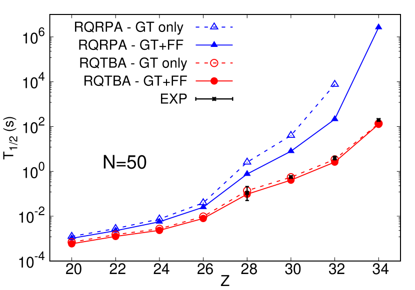
Figure 2: $\beta$-decay half-lives of $N=50$ isotones obtained within RQRPA (blue triangles) and RQTBA (red circles), in the allowed GT approximation (empty symbols) and including the FF transitions (full symbols). When no symbol is shown, the nucleus is predicted to be stable. The experimental data is taken from Ref. [57].

We show in Fig. 2 the $\beta$-decay half-lives of $N=50$ isotones obtained within RQRPA and RQTBA, i.e. without and with the QVC interaction $\Phi(\omega)$ in Eq. (LABEL:eq:BSE_pn), respectively. The empty symbols show the half-lives obtained in the allowed Gamow-Teller approximation, while the full symbols show the half-lives including the contribution of the first-forbidden transitions. We note that the effect of QVC becomes less and less important near the dripline since the decay $Q$ value is large. However the QVC is crucial closer to stability as the $Q$ value becomes small and thus the half-lives are very sensitive to the details of the transition strength distributions. In that case the correlations are able to reproduce the trend of the data to a much better extent. The half-life of ⁷⁸Ni is within the experimental error bar while those of $Z>28$ nuclei are slightly underestimated, up to $\simeq 34\%$ in the case of ⁸⁴Se.

We show in Fig. 3 the contribution $\lambda_{\text{FF}}/\lambda_{\text{tot}}$ (in percent) of the FF transitions to the total $\beta$-decay rate, in both RQRPA and RQTBA. We also show in this figure the individual contributions of the different multipoles $0^{-}$, $1^{-}$ and $2^{-}$.

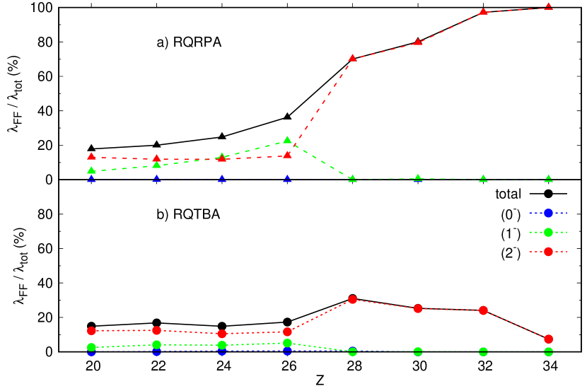
Figure 3: Contribution of first-forbidden transitions to the $\beta$-decay rate of $N=50$ nuclei (in $\%$) within a) RQRPA and b) RQTBA. The full contribution is shown with a plain black line while the dashed lines show the individual contribution of the different multipoles.

In order to understand the results, we analyze the transition densities of the different modes. To guide the reader in the following discussion, we show in Fig. 4 the single-particle spectrum of ⁷⁸Ni obtained in the RMF approximation with the NL3 functional.

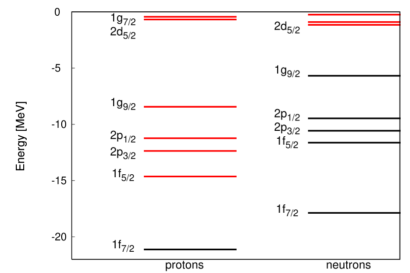
Figure 4: Single-particle spectrum in ⁷⁸Ni. The black levels are fully occupied, while the red ones are empty.

The RMF occupations of the neutron levels remain the same throughout the $N=50$ chain, while the occupations of the proton states change. In particular, the proton $1f_{7/2}$ is partially empty in isotones with $Z<28$, while it is basically fully filled in heavier isotones within the RMF.

In nuclei with $Z<28$, we find in both RQRPA and RQTBA a dominant contribution from Gamow-Teller modes to the total rate, mainly originating from the low-energy $\mathtt{n}1f_{5/2}\rightarrow\mathtt{p}1f_{7/2}$ transition, although the weight of FF modes increases to $\simeq 36\%$ at $Z=26$ in RQRPA. In both cases the contribution of $0^{-}$ modes is negligible (below $0.5\%$), as these transitions occur between states of same total angular momentum $j$ and different parity (e.g. $\mathtt{n}1d_{5/2}\rightarrow\mathtt{p}1f_{5/2}$, $\mathtt{n}2p_{1/2}\rightarrow\mathtt{p}2s_{1/2}$ and $\mathtt{n}2p_{3/2}\rightarrow\mathtt{p}1d_{3/2}$) and thus involve proton states that are almost fully occupied. RQTBA predicts a contribution from $1^{-}$ and $2^{-}$ modes of roughly the same order (3–12%), with the major transitions being $\mathtt{n}1g_{9/2}\rightarrow\mathtt{p}1f_{7/2}$ for the $1^{-}$ modes and $\mathtt{n}1g_{9/2}\rightarrow\mathtt{p}1f_{7/2,5/2}$ for the $2^{-}$ operator. To a lesser extent, but with a similar order of magnitude, the transition $\mathtt{n}2d_{5/2}\rightarrow\mathtt{p}1f_{7/2}$ also contributes to the $2^{-}$ modes. Such a transition is due to the presence of ground-state correlations which induce slight occupation of the neutron $2d_{5/2}$ sub-shell.

Since we do not include ground-state correlations (GSC) induced by QVC, these are caused by the GSC of the RQRPA (the usual “B” interaction matrix [14]). In RQRPA, the contribution of the rank-1 operators is slightly larger and increases with $Z$ (up to $22\%$ in ⁷⁶Fe) even though the occupation of the proton $1f_{7/2}$ becomes larger (this is because the decrease in GT contribution is stronger than the $1^{-}$ decrease, thus the relative contribution of $1^{-}$ goes up).

In nuclei with $Z\geq 28$, the proton $1f_{7/2}$ sub-shell becomes fully occupied, and transitions via rank-1 operators are blocked so that only $2^{-}$ modes generate FF transitions. The main low-energy Gamow-Teller transition $1f_{5/2}\rightarrow 1f_{7/2}$ is also blocked. In RQRPA, transitions between other sub-shells are located near the $Q$ value, which explains the small or absent contribution of GT transitions in nuclei with large $Z$. The correlations due to QVC lower down such transitions (in particular, $\mathtt{n}2p_{1/2,3/2}\rightarrow\mathtt{p}2p_{1/2,3/2}$, $\mathtt{n}1f_{5/2}\rightarrow\mathtt{p}2p_{3/2}$, $\mathtt{n}2p_{3/2}\rightarrow\mathtt{p}1f_{5/2}$, $\mathtt{n}1f_{5/2}\rightarrow\mathtt{p}1f_{5/2}$, or $\mathtt{n}1g_{9/2}\rightarrow\mathtt{p}1g_{9/2}$) so that within RQTBA, GT transitions contribute to $\gtrsim 70\%$ and thus remain dominant. The trend found in Fig. 3 in RQTBA is similar to the shell-model calculations of Ref. [39] for $Z<28$. For $Z\geq 28$, that reference finds a drop of the FF due to smaller contribution of the $2^{-}$ modes, which, are typically found at lower energies than in the present calculations (by $\simeq 2$ MeV). This is discussed further in the following paragraph.

Finally we show in Fig. 5 distributions of partial decay rates obtained within RQRPA (left panels) and RQTBA (right panels) in ⁷⁴Cr, ⁷⁸Ni and ⁸²Ge.

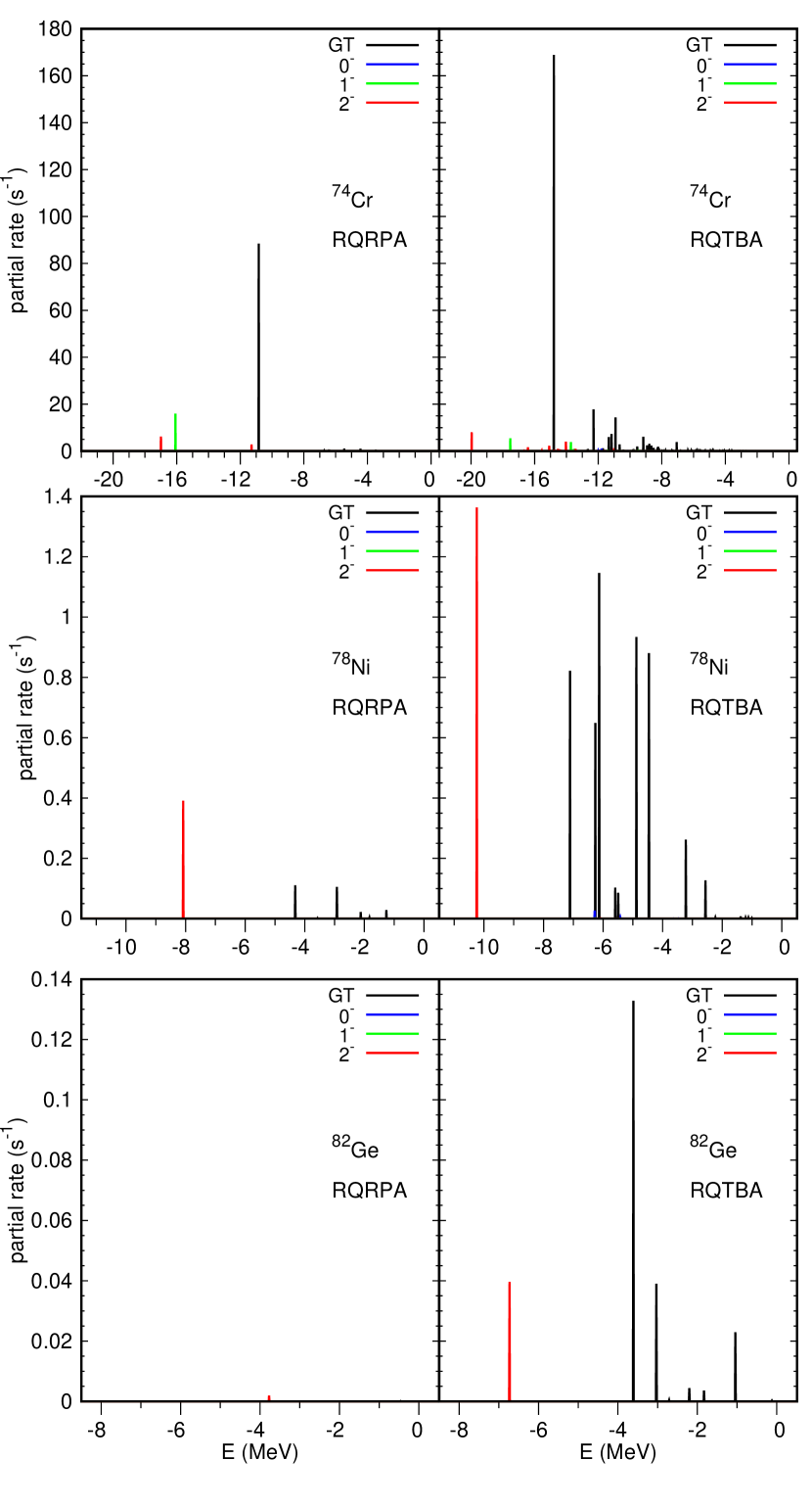
Figure 5: Distribution of partial rates (in $s^{-1}$) in ⁷⁴Cr, ⁷⁸Ni and ⁸²Ge in the decay window, within RQRPA (left panels) and RQTBA (right panels). The excitation energy (in MeV) is $E=E_{f}=M_{i}-M_{f}$ as defined in section II.

Clearly we see that GT transitions are almost absent from the decay window in RQRPA for large values of $Z$, while they are brought down in energy due to the fragmentation process induced by QVC. Overall we note that FF transitions appear at lower energy than the GT modes. This is in accordance with the shell model calculations of Ref. [39]. The details of the RQTBA partial rate distributions however present some discrepancies with those provided in that reference. In ⁷⁴Cr we find a large GT transition at $E_{f}\simeq-15.5$ MeV which appears to be split into two components in the shell model case. The rest of the distribution is fragmented over several states in both approaches. For $Z\geq 28$, we observe more dissimilarities between the two methods, in particular in ⁷⁸Ni. For this nucleus RQTBA shows a GT contribution which is quite fragmented as well as very large contribution from the low-lying $2^{-}$ state at $E_{f}\simeq-10.75$ MeV. The shell model of Ref. [39], on the other hand, predicts a GT strength that is concentrated in only a few peaks and a very small contribution of the $2^{-}$ mode. In ⁸²Ge, while the GT distributions are more similar, we also predict an important low-lying $2^{-}$ peak which is found to be almost negligible in the shell model. Overall, we note that our $2^{-}$ states seem to be predicted too low in excitation energy. For instance, the experimental $Q_{\beta}$ value for ⁸²Ge is $4.69$ MeV and the estimated value for ⁷⁸Ni is 9.91 MeV [58], while from Fig. 5 we see that our $Q_{\beta}$ values would be at least $\simeq 7.25$ MeV and $10.75$ MeV, respectively. Nevertheless, we find similar transition strengths to the low lying $2^{-}$ states that predicted by the shell-model. For ⁸²Ge RQTBA predicts a $\log f_{1}t=8.0$ while the shell-model calculations give $\log f_{1}t=8.3$ to the low lying $2^{-}$ state. Both compare well with the measured vaue of $\log f_{1}t=8.6(3)$ [59]. For ⁷⁸Ni the low lying $2^{-}$ state has a $\log f_{1}t=4.5$ both in the RQTBA and shell-model approaches. For ⁷⁴Cr we have $\log f_{1}t=8.6$ (RQTBA) and $\log f_{1}t=8.9$ (Shell-Model). The large $Q_{\beta}$ values are potentially caused by the fact that, in the present study, the QVC correlations are only included in the description of the daughter nucleus, and not in the parent ground state. Indeed it was observed in Ref. [36] that accounting for these ground-state correlations could potentially bring the binding-energy differences, and thus the $Q_{\beta}$ values, in better agreement with the data. Understanding in more details the differences between RQTBA and shell model calculations, for different truncations of the model spaces, and the role played by the ground-state correlations, will be the subject of a future study.

III.1.2 Isoscalar pairing interaction

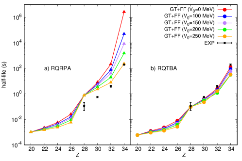
Figure 6: $\beta$-decay half-lives of $N=50$ isotones obtained within a) RQRPA and b) RQTBA, for different values of the static isoscalar pairing interaction $V_{0}$.

In the calculations that we have discussed so far, we have not included a $T=0$ proton-neutron ($pn$) particle-particle ($\mathfrak{p}\mathfrak{p}$) component (usually referred to as ”pairing” component) $\widetilde{V}_{pn}^{(\mathfrak{p}\mathfrak{p})(T=0)}$ of the static interaction. This is so because it does not contribute to the structure of the parent state in the RMF approximation. Thus, in standard QRPA calculations, this component is often adjusted a posteriori, when investigating the nuclear response [15, 18]. In RQRPA, a Gogny-type ansatz is often considered:

$$\widetilde{\bm{V}}_{pn}^{(\mathfrak{p}\mathfrak{p})(T=0)}=-V_{0}\sum_{j=1,2}g_{j}e^{-r_{pn}^{2}/\mu_{j}^{2}}\bm{\Pi}_{S=1,T=0}\;,$$ (41)

where $\bm{\Pi}_{S=1,T=0}$ projects onto states with $S=1$ and $T=0$, $\mu_{1}=1.2$ fm and $\mu_{2}=0.7$ fm are the range of the Gogny D1S force [60], and the relative strengths are chosen to be $g_{1}=1.0$ and $g_{2}=-2.0$ so that the interaction is repulsive at short distance. Such interaction then usually increases the beta strength at low-energy and yields a decrease of the half-lives. The remaining free parameter $V_{0}$ is then typically adjusted in order to reproduce the $\beta$-decay half-lives. However it was shown that the resulting value of this parameter can vary strongly according to the mass region and often has to be pushed close to the point of collapse of the theory, when adjusted at the RQRPA level [18]. These observations overall point out to the fact that by tuning $V_{0}$ to large values, one may be trying to correct for deficiencies of the model.

As a test, we include the interaction of the form (41) in our calculations, and vary the parameter $V_{0}$ to investigate the sensitivity of our half-lives to such particle-particle component of the static $T=0$ interaction, when QVC correlations are included. The results are shown in Fig. 6 in both RQRPA and RQTBA. First of all, we note that this interaction has no effect in ⁷⁸Ni and ⁷⁰Ca, and more generally in doubly-magic nuclei. This is because the transition matrix elements in the particle-particle channel come with factors $\sim v_{p}^{2}v_{n}^{2}$ and $\sim u_{p}^{2}u_{n}^{2}$ (where $v_{k}^{2}$ is the occupation of single-particle state $k$ and $u_{k}^{2}+v_{k}^{2}=1$) which are always zero in such nuclei.

In $Z>28$, $\widetilde{V}_{pn}^{(\mathfrak{p}\mathfrak{p})(T=0)}$ has much less effect in RQTBA than in RQRPA, in particular close to stability. Let us analyze the case of ⁸⁴Se. At the RQRPA level the main transition responsible for the decay is the $\mathtt{n}1g_{9/2}\rightarrow\mathtt{p}1f_{5/2}$ caused by the rank-2 operator. The corresponding particle-particle matrix element comes with a factor $v_{p}^{2}v_{n}^{2}=v_{p}^{2}$, which is large ($\simeq 0.88$) for ⁸⁴Se as the proton $1f_{5/2}$ is largely occupied. Thus, the T=0 particle-particle interaction has a large effect for this nucleus. In RQTBA, the decay in this nucleus is caused by GT transitions by more than $95\%$ in agreement with experimental data, with the main contributions caused by transitions between the neutron and proton $2p_{1/2,3/2}$ sub-shells. Since the occupation of these proton levels are small ($v_{p}^{2}\simeq 0.1$ and $0.05$) the $T=0$ particle-particle static interaction is much less effective, which is why the half-lives of ⁸⁴Se, and other $Z>28$ nuclei, are more stable against variations of the strength $V_{0}$ of this interaction than within RQRPA.

For $Z<28$ isotones, however, the effect of $\widetilde{V}_{pn}^{(\mathfrak{p}\mathfrak{p})(T=0)}$ appears similar with and without QVC. For these nuclei, both GT and FF ($1^{-}$ and $2^{-}$) modes contribute in RQRPA and RQTBA, and the most important transitions involve the proton $1f_{7/2}$ sub-shell which has $v_{p}^{2}$ varying from $0.25$ in ⁷²Ti to $0.74$ in ⁷⁶Fe. Therefore the effect of $\widetilde{V}_{pn}^{(\mathfrak{p}\mathfrak{p})(T=0)}$ increases with $Z$ and is found similar at both levels of approximation.

Clearly it seems difficult to find a single value of $V_{0}$ for which RQRPA would reproduce the experimental half-lives of the whole chain. In particular it is not possible for ⁷⁸Ni which is doubly-magic, and thus insensitive to the proton-neutron pairing interaction. In RQTBA, the data is best reproduced for $V_{0}$=0, but as noted above, varying this parameter has little effect for $Z\geq 28$, and we cannot conclude for $Z<28$ since no data is available.

For these reasons, and because we find similar results as Fig. 6 for other isotonic chains, we will consider $V_{0}=0$ in the rest of this manuscript. We point, however, that the proton-neutron particle-particle channel is still taken into account via the dynamical QVC interaction $\Phi(\omega)$ (see Eq. LABEL:eq:Phi). This may explains why the QVC results agree well with the data, without having to resort to static $T=0$ particle-particle interaction.

III.2 $N=82$ chain

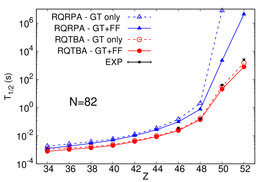
Figure 7: $\beta$-decay half-lives of $N=82$ isotones obtained within RQRPA (blue triangles) and RQTBA (red circles), in the allowed GT approximation (empty symbols) and including FF transitions (full symboles). When no symbol is shown, the nucleus is predicted to be stable. The experimental data is from [57].

We show in Fig. 7 the half-lives of $N=82$ isotones. As in the $N=50$ chain, the effect of QVC correlations is very important closer to stability, as it reduces the half-lives by several orders of magnitudes and leads to a much better agreement with the available data, although the reduction tends to be slightly too strong in some cases. As one goes towards the neutron dripline (towards small $Z$), the effect of QVC on the half-lives fades out and the predictions of RQTBA become similar to the ones of RQRPA.

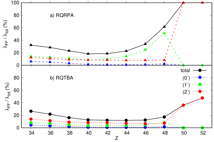
Figure 8: Contribution of first-forbidden transitions to the $\beta$-decay rate of $N=82$ nuclei (in $\%$) within a) RQRPA and b) RQTBA. The full contribution is shown with a plain black line while the dashed lines show the individual contribution of the different multipoles.

We show in Fig. 8 the contribution of first forbidden transitions to the $\beta$-decay rates. In nuclei with $Z\geq 40$, $pf$-shell orbits for protons are, to first approximation, fully occupied. This suppresses $0^{-}$ transitions (e.g. $\mathtt{n}2d_{3/2}\rightarrow\mathtt{p}2p_{3/2}$ or $\mathtt{n}2d_{5/2}\rightarrow\mathtt{p}1f_{5/2}$). In lighter isotones, while the transition $\mathtt{n}2d_{3/2}\rightarrow\mathtt{p}2p_{3/2}$ is Pauli un-blocked, we find that the contribution of $0^{-}$ modes to the rate remains small (below $6\%$) due to a strong cancellation between the spin-dipole component, Eq. (13), and the relativistic one, Eq. (24). In nuclei with $Z\leq 42$, the decay proceeds essentially via GT (mostly $\mathtt{n}1g_{7/2}\rightarrow\mathtt{p}1g_{9/2}$), with a comparable contribution of $1^{-}$ and $2^{-}$ modes below $\simeq 14\%$ at both levels of approximations.

In heavier isotones with $Z\geq 44$, the $1^{-}$ component increases in RQRPA, via transition $\mathtt{n}1h_{11/2}\rightarrow\mathtt{p}1g_{9/2}$, until $Z=50$ when the proton $1g_{9/2}$ becomes fully filled. The main low-energy GT and $1^{-}$ transitions are then completely blocked and the decay proceeds solely via rank-$2$ FF transitions (mostly $\mathtt{n}1h_{11/2}\rightarrow\mathtt{p}1g_{7/2}$).

Within RQTBA, the trend is changed in nuclei with large $Z$, where the GT remains the largest contribution ($>50\%$), even above the $Z=50$ shell closure. In such nuclei, even though the proton $1g_{9/2}$ is filled, GT modes caused by transitions such as $\mathtt{n}1h_{11/2}\rightarrow\mathtt{p}1h_{11/2}$ or $2d_{3/2}\rightarrow 2d_{5/2}$ are lowered in energy due to QVC, and contribute significantly to the decay because of the phase space.

The RQRPA and RQTBA partial decay-rate distributions of ¹¹⁸Kr, ¹²⁴Mo and ¹³²Sn are shown in Fig. 9.

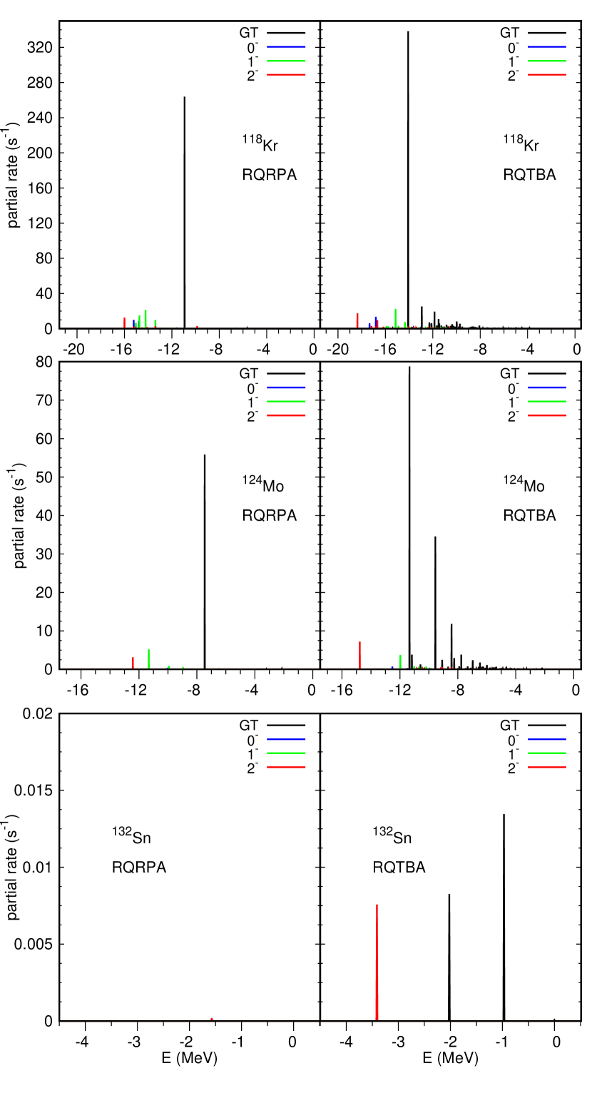
Figure 9: Distribution of partial rates (in $s^{-1}$) for ¹¹⁸Kr, ¹²⁴Mo and ¹³²Sn in the decay window, within RQRPA (left panels) and RQTBA (right panels). The excitation energy (in MeV) is $E=E_{f}=M_{i}-M_{f}$ as defined in section II.

In ¹¹⁸Kr the transitions of RQRPA and RQTBA actually show a similar profile (with a bit more fragmentation in RQTBA), however the shift due to QVC towards lower energy enhances the contributions to the rates due to the phase space. In ¹²⁴Mo and ¹³²Sn, the effect of QVC grows greatly. As in the $N=50$ chain, FF transitions overall occur at lower energy than GT modes. We note that the distribution in ¹²⁴Mo has a similar profile than the shell model calculation of Ref. [39], however the first FF transition occurs $~{}2$ MeV lower in our calculation.

III.3 $N=126$ chain

Fig. 10 shows the $\beta$-decay half-lives of $N=126$ isotones.

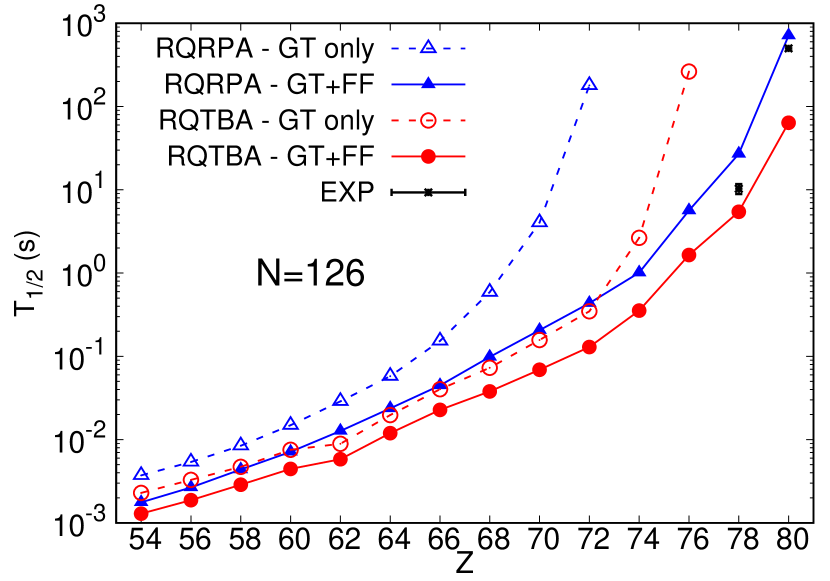
Figure 10: $\beta$-decay half-lives of $N=126$ isotones obtained within RQRPA (blue triangles) and RQTBA (red circles), in the allowed GT approximation (empty symbols) and including FF transitions (full symboles). When no symbol is shown, the half-life is predicted to be infinite. The experimental data is from [57].

In this chain, while QVC is important near stability in the allowed GT approximation (empty symbols), its effect is reduced to about one order of magnitude at most when FF transitions are included. Again, the too strong decrease of the half-lives due to QVC observed in ²⁰⁴Pt and ²⁰⁶Hg could potentially be explained by the fact that, in the present study, we do not include ground-state correlations induced by QVC. These correlations, that were implemented and investigated in doubly-magic nuclei [36], can lead to a small shift of the strength back to higher energy, re-increasing slightly the half-lives. The effect of such correlations in the parent ground state of open-shell nuclei will be investigated in the future. We also note that, for these nuclei, FF transitions contribute to the decay rate by a large fraction (see below) and we have not applied any quenching to FF modes either.

In Fig. 11 is shown the contribution of FF transitions to the rates.

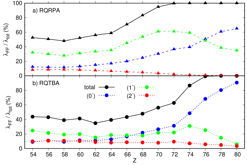
Figure 11: Contribution of first-forbidden transitions to the total $\beta$-decay rate of $N=126$ nuclei (in $\%$) within a) RQRPA and b) RQTBA.

The probability for the decay to occur via FF transitions is very large throughout the chain, in both RQRPA and RQTBA. The total contribution in the region far from stability is about $\sim 50-60\%$ in RQRPA, and $\sim 35-45\%$ in RQTBA. Above $Z\geq 68$ the proton $1h_{11/2}$ becomes more occupied and the main low-energy GT transition $\mathtt{n}1h_{9/2}\rightarrow\mathtt{p}1h_{11/2}$ is blocked by the Pauli principle. This explains the increase of the FF contribution towards stability. As will be discussed in section IV, such an increase has also been observed in other theoretical methods. However, the steepness of the increase and the overall contribution of the FF transitions in the $N=126$ isotonic chain, especially towards the neutron dripline, strongly varies between the different models.

Similarly to Ref. [39], we find that FF transitions are dominated in these $N=126$ isotones by $0^{-}$ and $1^{-}$ modes, while contributions of $2^{-}$ transitions are very small throughout the chain. The main single-particle transitions contributing to FF modes involve (in order of increasing energy) the proton $2d_{5/2}$, $1h_{11/2}$, $2d_{3/2}$ and $3s_{1/2}$. For low values of $Z$, these sub-shells are mostly empty and leading to more available $1^{-}$ than $0^{-}$ transitions, based on selection-rules arguments. As the proton number $Z$ increases, these sub-shells are gradually filled, until the $\mathtt{p}2d_{3/2}$. In that case the main remaining transition is $\mathtt{n}3p_{1/2}\rightarrow\mathtt{p}3s_{1/2}$ which contributes to both $0^{-}$ and $1^{-}$. The $0^{-}$ decay becomes more probable as the corresponding daughter states appear lower in energy, as can be seen from, e.g., Fig.12. In contrast, the shell-model calculations of Ref. [39] found a dominance of the rank-1 operators ($\simeq 70\%$ of the FF) over the rank-0 transitions in the range $66\leq Z\leq 72$.

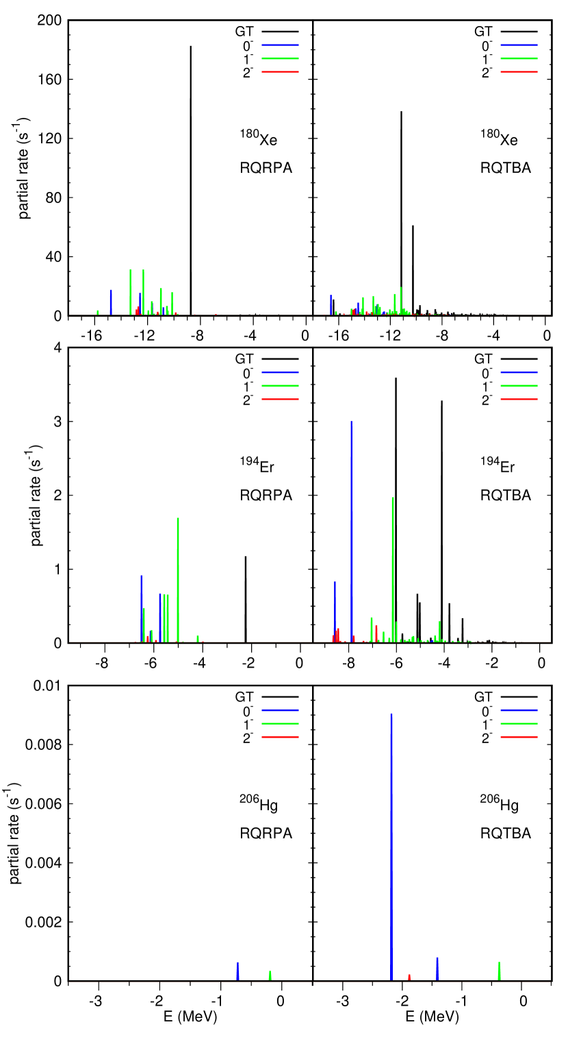
Figure 12: Distribution of partial rates (in $s^{-1}$) for ¹⁸⁰Xe, ¹⁹⁴Er and ²⁰⁶Hg in the decay window, within RQRPA (left panels) and RQTBA (right panels). The excitation energy (in MeV) is $E=E_{f}=M_{i}-M_{f}$ as defined in section II.

As mentioned in section II.1, $0^{-}$ transitions have two components: one originates from the spin-dipole operator, $w$ and $w^{\prime}$ terms in Eqs. (13,17), while the other is due to the relativistic $\gamma_{5}$ operator, $\xi^{\prime}v$ term in Eq. (24), which originates from the time-like part of the axial current. Because of interference between them, it is difficult to disentangle the effects of these two contributions. This topic has been intensely studied by Warburton within a shell-model framework [44]. He found that there is typically a strong cancellation between the spin-dipole and $\xi^{\prime}v$ terms, and thus, that an enhancement of $\xi^{\prime}v$ is necessary to avoid such cancellation. In particular, an enhancement factor of $\sim 2$ was needed in the lead region. Generally, even though the enhancement factor varies between different approaches, it is agreed that the predictions of methods based on impulse approximation within a non-relativistic formalism typically largely underestimate the relative contribution the $\xi^{\prime}v$ term. While an important part of this enhancement in principle originates from two-body, or meson-exchange currents, as originally demonstrated by Kubodera et al. based on chiral-symmetry arguments [61], a substantial portion of it may also originate from other effects, such as relativistic corrections [44].

In our calculation, we also find that both spin-dipole and $\xi^{\prime}v$ terms interfere destructively. To investigate this aspect further, we try to evaluate the importance of both spin-dipole and $\xi^{\prime}v$ components and show in Fig. 13, the $\beta$-decay rate $\lambda_{0^{-}}$ originating from the $0^{-}$ transitions, obtained when suppressing one of the two components.

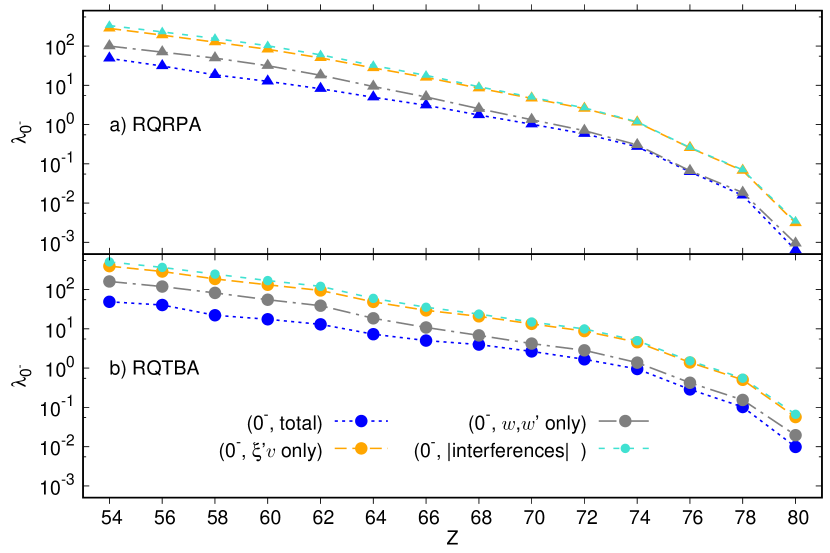
Figure 13: $\beta$-decay rates from the $0^{-}$ transitions of $N=126$ nuclei (in $\%$) within a) RQRPA and b) RQTBA. The blue symbols show the full $\lambda_{0^{-}}$ rates, the orange and grey symbols show the rates obtained when including only the relativistic ($\xi^{\prime}v$) and spin-dipole ($w$ and $w^{\prime}$) components, respectively. The turquoise symbols show the contribution of the absolute value of the destructive interference term.

Specifically, the orange and grey symbols show the rates obtained when including only the relativistic ($\xi^{\prime}v$) and spin-dipole ($w$ and $w^{\prime}$) components, respectively. The turquoise symbols show the absolute value of the destructive interference term. It appears that both components contribute by a similar order of magnitude, with a somewhat larger contribution of the relativistic operator (factor $\simeq 2-3$ in the rate). The interference term is negative and also of the same order (with a value comparable to the relativistic term). Consequently, $\lambda_{0^{-}}$ also takes a value of the same order of magnitude. As a reminder, no quenching or enhancement factors have been applied in the present study. It would be interesting to investigate further the contribution of the different components and their interference in a shell-model framework. We leave such study for a future work.

III.4 $N=184$ chain

We show in Figs. 14 and 15 the $\beta$-decay half-lives and contribution of FF transitions of $N=184$ isotones, respectively. We note that ²⁹⁰Sg ($Z=106$) has been treated here without pairing correlations, due to a failure (collapse) of the numerical procedure for that nucleus. This explain the non-smooth behaviour of some curves around $Z=106$.

Overall, the effect of QVC is of several orders of magnitude near stability, and the FF transitions largely dominate the decay, except close to stability in RQTBA.

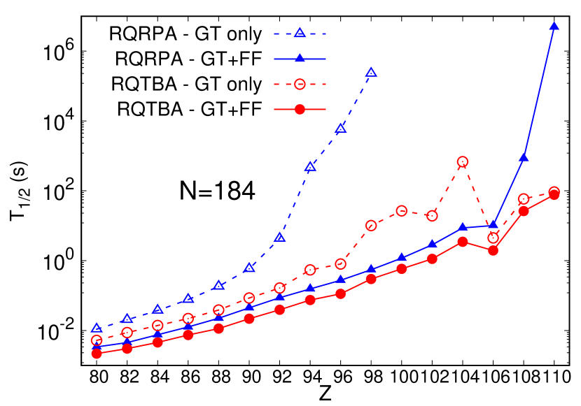
Figure 14: $\beta$-decay half-lives of $N=184$ isotones obtained within RQRPA (blue triangles) and RQTBA (red circles). The empty symbols show the half-lives obtained in the allowed Gamow-Teller approximation, while the full symbols show the half-lives with the contribution of the first-forbidden transitions.

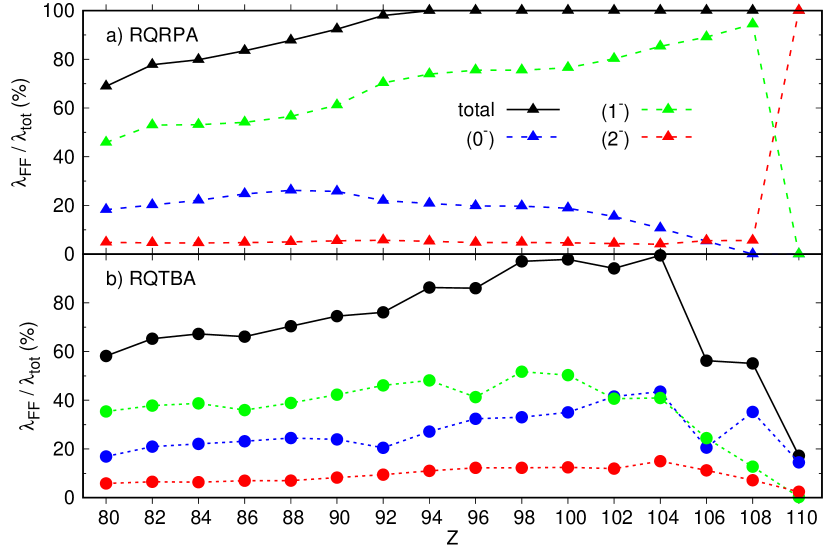
Figure 15: Contribution of first-forbidden transitions to the total $\beta$-decay rate of $N=184$ nuclei (in $\%$) within a) RQRPA and b) RQTBA.

At the RQRPA level, the FF contribution remains above $\gtrsim 70\%$ throughout the chain, and increases with $Z$ as the main GT transition $\mathtt{n}4s_{1/2}\rightarrow\mathtt{p}3s_{1/2}$ becomes blocked due to the filling of the $\mathtt{p}3s_{1/2}$ level. Note that such transitions between states with different main quantum numbers $n$ is only allowed due to isospin-breaking terms of the interaction, in particular, the Coulomb force. For nuclei with $Z\geq 92$, the decay is basically of purely forbidden nature. Throughout the chain the decay proceeds mostly via rank-1 operators ($\mathtt{n}3d_{3/2,5/2}\rightarrow\mathtt{p}2f_{5/2,7/2}$) which are responsible for about $45-95\%$ of the total rate, with an increasing contribution towards stability until $Z=108$. Rank-0 operators contribute to about $20\%$ far from stability (via $\mathtt{n}2g_{9/2}\rightarrow\mathtt{p}1h_{9/2}$) and become unimportant near stability. In that region, only few transitions occur below the decay $Q$ value. In particular, in $Z=110$, almost all transitions appear above that value, except for a very small $2^{-}$ state which corresponding partial rate is negligible ($\sim 10^{8}$) and not visible on Fig. 16.

At the RQTBA level, the total contribution of FF modes is of similar magnitude up to $Z=104$ $\gtrsim 70\%$, after which it decreases to a value of $\simeq 17\%$ at $Z=110$. In the three isotones closest to stability some GT transitions are lowered down in energy due to the correlations introduced by the QVC, in particular, $\mathtt{n}1i_{11/2}\rightarrow\mathtt{p}1i_{13/2}$, as well as $\mathtt{n}2h_{9/2}\rightarrow\mathtt{p}2f_{7/2}$. Note that the latter transition is due to GSC included in RQRPA, combined with QVC effects. Overall the contribution of $0^{-}$ (and $2^{-}$) modes is enhanced compared to RQRPA, especially at large $Z$, while the contribution of $1^{-}$ modes is decreased. This is similar to the behaviour observed in the $N=126$ chain.

Finally we show in Fig. 16 the distribution of partial decay rates within RQRPA and RQTBA in ²⁶⁴Hg, ²⁸⁰Hg and ²⁹⁴Ds, where one can again appreciate the importance of FF transitions. In ²⁹⁴Ds we also note a strong GT transitions which appears at lower energy than the FF one.

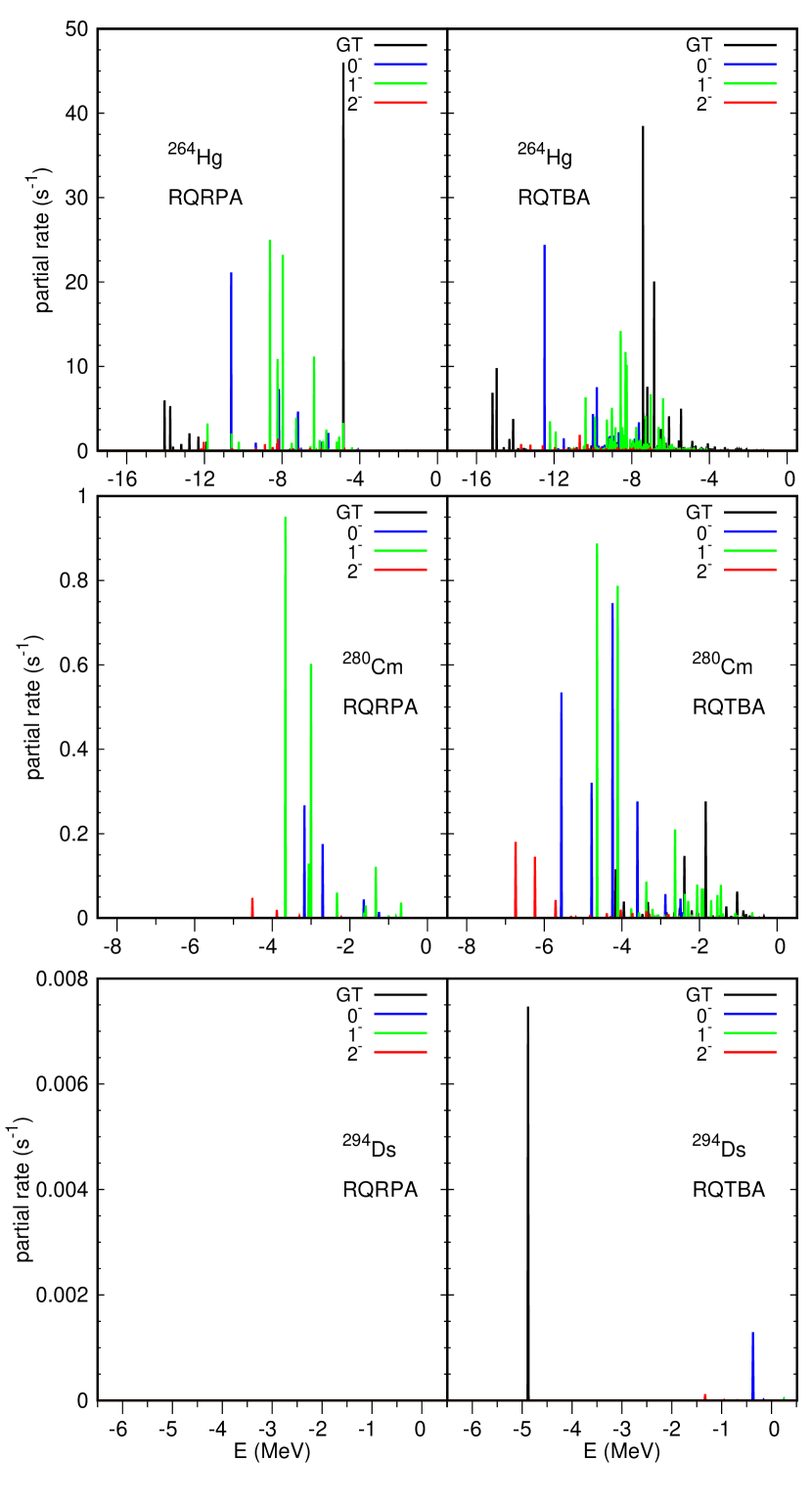
Figure 16: Distribution of partial rates (in $s^{-1}$) for ²⁶⁴Hg, ²⁸⁰Cm and ²⁹⁴Ds in the decay window, within RQRPA (left panels) and RQTBA (right panels). The excitation energy (in MeV) is $E=E_{f}=M_{i}-M_{f}$ as defined in section II.

IV Comparison with other approaches

We now compare our results, obtained at the RQTBA GT+FF level, to other existing calculations. The left panels of Fig. 17 show a comparison of the $\beta$-decay half-lives for the four isotonic chains under study, while the right panels compare the total contributions of the FF transitions to the rates.

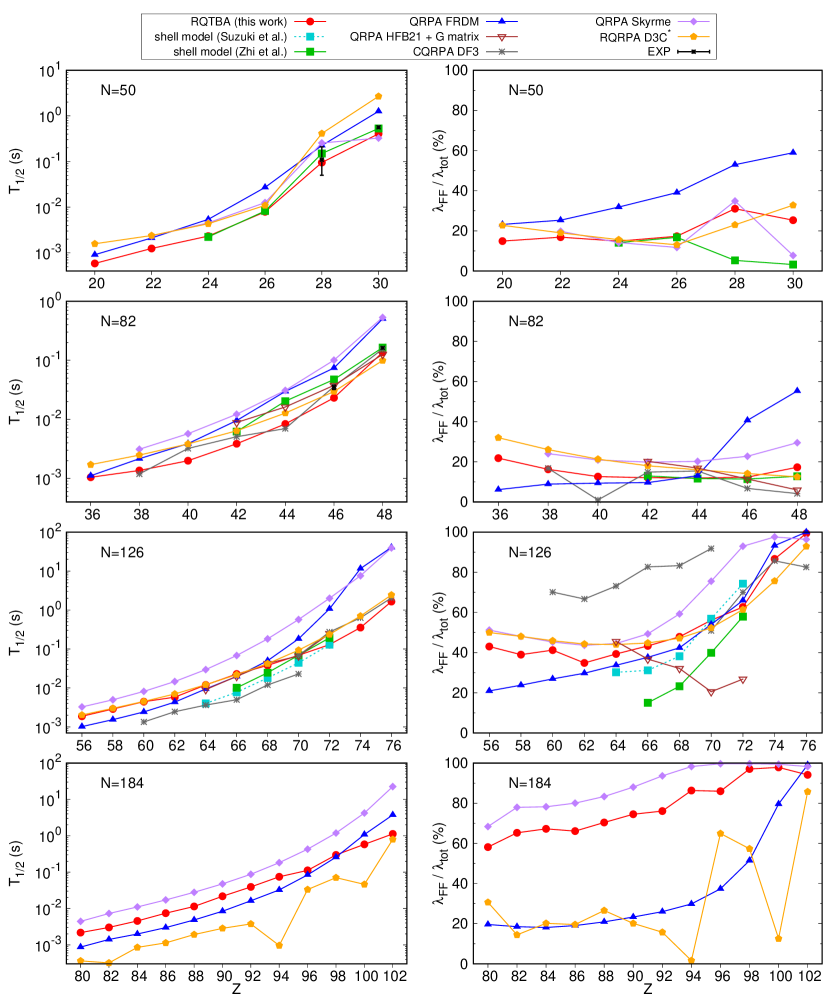
Figure 17: Comparison of our results (red circles) with other theoretical calculations from shell models and various QRPA approaches. The left panels show a comparison of the $\beta$-decay half-lives and the right panels show a comparison of the predicted contributions of FF transitions. See text for explanations of the different theoretical models. The experimental data is from [57].

In these figures we selected nuclei with a half-life between $\sim 1$ ms and $1$ s, which are those of interest for the $r$ process. We include results obtained within the shell model and various QRPA calculations, specifically:

• the shell model calculations of Ref. [38] (’Suzuki et al.’, turquoise squares),

• the shell model calculations of Ref. [39] (’Zhi et al.’, green squares), which used a larger model space as well as a different effective interaction,

• the QRPA calculation of Ref. [17] based on FRDM (’FRDM’, blue triangles) using a schematic interaction and combining microscopic calculation of GT modes and macroscopic description of FF transitions,

• the microscopic (but non self-consistent) QRPA calculation of Ref. [21] (’HFB21 + G matrix’, empty brown triangles) based on a G-matrix derived from the realistic CD-Bonn interaction [62], using single-particle energies obtained from a Skyrme functional and the HFB21 mass model [63] for the calculation of unknown Q values (similar results were also obtained with the FRDM mass model and are not shown here),

• the non-relativistic microscopic self-consistent continuum QRPA calculations of Refs. [16, 64] using DF3 [65] Fayans functional (’DF3’, grey stars),

• the non-relativistic microscopic self-consistent deformed QRPA approach using SkO’ [66] Skyrme functional of Ref. [24] (’Skyrme’, purple diamonds),

• the relativistic microscopic self-consistent spherical QRPA approach using D3C^∗ [67] functional of Ref. [13] (’D3C^∗’, orange pentagons). Note that the results shown here differ slightly from Ref. [13] due to corrected phases in the computer code.

These QRPA calculations differ from the ones we have shown previously by the fact that some of them are not fully microscopic and/or self-consistent, they use different interactions or functionals (relativistic or not) and they all include residual (static) isoscalar proton-neutron pairing interaction which is typically fitted in different ways to reproduce known $\beta$-decay half-lives. Some of the non-relativistic QRPA’s also treat further effects such as deformation or continuum.

We also note that the methods we are comparing use different values for the quenching of the different multipole modes contributing to the decay. In particular, all the microscopic approaches apply a quenching $q$ to the Gamow-Teller transitions, ranging from $q=0.4$ in the QRPA of Ref. [21], to $q\simeq 0.7$ in the shell model calculations  [38, 39], and $q\simeq 0.78$ (amounting to using $g_{A}\simeq-1.0$) in the remaining self-consistent QRPA calculations [16, 64, 24, 13].

The quenching of FF transitions is however handled much differently. In the shell model of Ref. [39], the quenching (or enhancement for the $0^{-}$ operator) of the different multipoles contributing to FF modes are fixed to reproduce known $\beta$-decay half-lives. In the shell model of Ref. [38], the FF contributions are quenched in the same way as the GT, except the $0^{-}$ modes which are enhanced (by a factor $2$ for the relativistic component). The QRPA calculations of Ref. [13] and Ref. [16] use the same quenching for all GT and FF transitions, while Ref. [24] keeps the bare FF channel [68]. Finally, Ref. [21] quenches the FF modes by a factor $0.5$ except the rank-0 operators that are enhanced. As a reminder, the present RQTBA results are obtained without any quenching, neither in the GT nor in the FF cases, using the current bare value $g_{A}=-1.27641$ [69].

In the $N=50$ isotonic chain the RQTBA half-lives are very similar to those predicted by the shell model. The contributions of FF transitions are also of the same order of magnitude although the shell model predicts a decrease of FF contribution above $Z=28$, while it increases by a few percents in RQTBA, due to low-lying $2^{-}$ transitions in this region, as discussed previously in section III.1. The QRPA calculations typically predict larger half-lives than RQTBA and shell model (except for the $Z=30$ case with Skyrme QRPA).

In the $N=82$ chain, RQTBA predicts half-lives that are lower than other calculations in the middle of the chain, except for a few exceptions. In particular, they are lower than the shell-model predictions by up to a factor $\simeq 2.4$. The contribution of FF transitions is predicted to be below $\simeq 32\%$ by all the microscopic approaches (except the FRDM QRPA near stability which predicts a larger probability for $Z=46-48$), with a spread of the results which grows towards the dripline, where FF transitions can be unlocked by growing neutron excess, and close to stability where they can become relatively important due to blocking of GT transitions.

In the $N=126$ chain the spread in the predictions of the half-lives reaches $\sim$ one to two orders of magnitude. The right panel of Fig. 17 shows a considerable spread in the predictions of FF modes contribution along the $N=126$ chain. In the range $Z=64-76$, almost all models (except Ref. [21]) predict an increase of the FF contribution due to the blocking of the $\mathtt{n}1h_{9/2}\rightarrow\mathtt{p}1h_{11/2}$ GT transition, as discussed previously in section III.3, but the steepness of this increase varies depending on the models. Shell-model calculations predict smaller probabilities for the FF decay in the middle of the chain, compared to (R)QRPA and RQTBA caluclations.

Due to computational limits the $N=184$ nuclei cannot be calculated by the shell model. However they have been computed by several QRPA methods. Overall the spread in the predicted half-lives is of $\sim$ two orders of magnitude. The Skyrme QRPA and RQTBA calculations appear to agree on a large contribution of the FF modes and on the trend along the chain (with a somewhat larger contribution predicted by the Skyrme QRPA by up to $\simeq 10-15\%$). The half-lives, however, differ by about one order of magnitude near stability. FRDM, on the other hand, predicts a low FF contribution of $20-30\%$ in the $Z=80-94$ range which then grows towards stability. The relativistic QRPA calculation with D3C^∗ provides FF contributions that are similar to the FRDM QRPA for most nuclei, but somehow shows strong variations, due to particularly strong GT contributions in $Z=94$ and $Z=100$ nuclei, which decrease the relative importance of the FF modes.

V Conclusion

In this paper we have performed systematic calculations of $\beta$-decay half-lives of even-even $r$-process waiting-point nuclei with $N=50$, $82$, $126$ and $184$ in the approach based on relativistic QRPA extended to include quasiparticle-vibration coupling (RQTBA). The calculations are based on the NL3 relativistic functional, with both allowed Gamow-Teller and first-forbidden transitions included.

Overall we found that the coupling between nucleons and vibrations, which typically induces fragmentation and spreading of the transitions strength distributions, leads to a decrease of the $\beta$-decay half-lives which is particularly important when the neutron excess is not too large and the decay $Q$ value is small.

In particular, in the $N=50$ and $N=82$ nuclei close to stability, the QVC is responsible for the appearance of GT transitions which then dominate the decay, in accordance with shell-model studies. The $\beta$-decay half-lives predicted by the RQTBA approach agree well with available experimental data in these lighter nuclei, without introducing extra quenching of the transition matrix elements. This demonstrates the ability of the present approach to capture correlations that are essential for a precise description of charge-exchange modes at low energy and accurate predictions of $\beta$-decay.

In the heavier nuclei, however, the decrease of the half-lives by QVC can be too strong and RQTBA tends to underestimate the available shell-model and (very few) experimental half-lives. This could be due to a too strong shift of the low-lying transition strength distributions towards lower energies due to missing ground-state correlations induced by QVC. Such correlations have been developed and implemented for doubly-magic nuclei and their impact on GT modes in ⁹⁰Zr was investigated in Ref. [36]. While we found that these GSC are mostly crucial for the description of the GT⁺ transitions, it was seen that they can also induce modifications of the GT^- strength, in particular, a small shift of the low-lying states back to higher energy. Such shift could thus potentially correct the too strong decrease of the half-lives observed in some cases of the present study. The effect of such correlations on the description of $\beta$-decay of selected nuclei should be investigated in a future paper.

The competition between GT and FF transitions in the present approach was also analyzed in detail. Overall the fragmentation induced by QVC was found to decrease the contribution of FF modes near stability, compared to RQRPA alone, which typically predicts very few GT states contributing to the decay, due to small decay $Q$ values. The contribution of FF modes was found to be below $\simeq 20-30\%$ in most $N=50$ and $N=82$ nuclei when QVC is included, with an increase towards the dripline and near stability in $N=82$, up to a value of $\simeq 50\%$. In the heavier nuclei, the probability of decay via FF transition was found to be greater, with a contribution of more than $\simeq 40-50\%$ up to $100\%$ in the $N=126$ chain, and a contribution of more than $\simeq 60\%$ in the $N=184$ chain (except near stability due to appearance of GT strength from QVC).

While in the light systems, $N=50$ and $N=82$, FF modes largely originate from rank-2 operators, we found that $1^{-}$ and $0^{-}$ modes contribute the most in heavy nuclei. Investigation of the rank-0 operator in $N=126$ showed a similar contribution from the spin-dipole component, relativistic component, and their destructive interference term (in absolute value). More detailed comparisons of the FF transitions components with shell-model calculations are planned for a next study.

Comparisons with precise theoretical methods, which include detailed nucleonic correlations, will provide guidance for future developments of the present approach. At the same time, upcoming experimental measurements of $\beta$-decay half-lives in the $N=126$ region by radioactive-beam facilities such as FAIR [70] will be crucial to test the reliability of the present approach in the heavy region. In the future we plan to extend this method to deformed nuclei and to perform global calculations of $\beta$-decay rates for $r$-process simulations.

Appendix A Calculations of first-forbidden transitions

We first recall a few aspects of the general response formalism, which can also be found in the literature (see e.g. Ref. [14]). Subsequently we expand on the calculation of FF transitions in this formalism.

A.1 General response formalism and transition strength distribution

The response formalism is based on the calculation of the transition strength distribution associated to a (one-body) given transition operator $\bm{O}$

$$S(\bm{O},E) = \sum_{f}|\braket{f}{\bm{O}}{i}|^{2}\delta(E-E_{f})\,,$$ (42)

$$= \frac{-1}{\pi}\lim_{\Delta\rightarrow 0}\mbox{Im}\sum_{f}\frac{|\braket{i}{\bm{O}}{f}|^{2}}{\omega-{E}_{f}}\,$$

$$= -\frac{1}{\pi}\lim_{\Delta\rightarrow 0^{+}}\mbox{Im }\,\Pi(\bm{O},\omega)\;,$$

with $\omega=E+i\Delta$, and where we have introduced the polarizability $\Pi(\omega,\bm{O})$ defined as

$$\Pi(\bm{O},\omega) = \sum_{f}\frac{|\braket{i}{\bm{O}}{f}|^{2}}{\omega-{E}_{f}}$$

$$= \braket{i}{\bm{O}^{\dagger}\bm{R}(\omega)\bm{O}}{i}\;,$$

where $\bm{R}(\omega)=1/(\omega-\bm{H}(\omega))$, where $\bm{H}(\omega)$ denotes the Hamiltonian of the system (which can be energy-dependent depending on the adopted many-body approximation).

Expressing the polarizability in single a quasiparticle basis $i=\{\eta_{i},k_{i}\}$, with $k_{i}=\{n_{i},\pi_{i},j_{i},\tau_{i}\}$

$$\Pi(\bm{O},\omega) = \sum_{1234}O_{12}^{*}R_{1423}(\omega)O_{34}\;,$$ (44)

where the response function $R_{1423}(\omega)$ is given by

$$R_{1423}(\omega) = \braket{i}{a_{2}^{\dagger}a_{1}\bm{R}(\omega)a_{3}^{\dagger}a_{4}}{i}$$ (45)

$$= \sum_{f}\frac{\braket{i}{a_{2}^{\dagger}a_{1}}{f}\braket{f}{a_{3}^{\dagger}a_{4}}{i}}{\omega-E_{f}}$$

As in the main text, in the case where $\bm{O}$ is a charge-exchange (GT or FF) transition operators, odd (resp. even) numbers will denote proton (resp. neutron) states.

In an angular-momentum coupled form, the polarizability reads

$$\Pi(\bm{O}^{J},\omega) = \braket{i}{\bm{O}^{J\,\dagger}\bm{R}^{J}(\omega)\bm{O}^{J}}{i}\;,$$ (46)

$$= \sum_{(1234)}O_{(12)}^{J,*}R_{(1423)}^{J}(\omega)O_{(34)}^{J}\;.$$

where $(i)=\{\eta_{i},n_{i},j_{i},\pi_{i},\tau_{i}\}$, and where the coupled response function $R_{(1423)}^{J}(\omega)$ is given by

$$R_{(1423)}^{J}(\omega)=(2J+1)\sum_{m_{1},m_{2},m_{3},m_{4}}(-1)^{j_{1}-m_{1}}(-1)^{j_{3}-m_{3}}$$

$$\hskip 14.22636pt\times\begin{pmatrix}j_{1}&j_{2}&J\\ m_{1}&-m_{2}&M\end{pmatrix}\begin{pmatrix}j_{3}&j_{4}&J\\ m_{3}&-m_{4}&M\end{pmatrix}R_{1423}(\omega)\;.$$

The equations above are general, and in the present framework, the response function is calculated by including QVC effects, as described in section II.

A.2 First-forbbiden transitions in the response formalism

The FF transitions include interference terms between operators of the same rank. Such terms can be calculated directly if one has access to the transition density matrices $\rho({\bm{O}^{J}})_{k_{1},k_{2}}=\braket{f}{\bm{O}^{J}}{i}$ associated to the various transition operators $\bm{O}$. In Ref. [71] a formula is provided which relates the transition strength distribution to the transition density matrix, however this expression is defined only up to a phase, and therefore does not allow to compute the sign of the interferences. Thus, in the response formalism, one has to find an alternative way to compute the FF transitions. A procedure was described in Ref. [56], and involves the computation of mixed transition strength distributions. Here we largely follow this procedure and adapt it to the present framework, which does not involve contour integrations as in Ref. [56]. We provide more details below.

As discussed in section II.1, the beta-decay rate associated with FF transitions is given by

$$\lambda_{\text{tot}} = \frac{\mbox{ln 2}}{K}\sum_{f,E_{f}<m_{e}}\int_{1}^{W_{f}}dWW\sqrt{W^{2}-1}(W_{f}-W)^{2}$$ (48)

$$\hskip 56.9055pt\times F(Z+1,W)\,C_{\text{FF}}(W)\;,$$

where $W=E_{e}/m_{e}$, $W_{f}\equiv(M_{i}-M_{f})/m_{e}=-(E_{f}/m_{e})$, with $M_{i}$ and $M_{f}$ the initial and final nuclear masses, repectively, and $F(Z+1,W)$ is the Fermi function [40]. The energy-dependent forbidden shape factor $C_{\text{FF}}(W)$ is a sum of four terms:

$$C_{\text{FF}}(W)=k+ka\,W+kb\,W^{-1}+kc\,W^{2}\;.$$ (49)

where $k,\;ka,\;kb,\;kc$ are given in Eq. (6)-(9).

Below we consider separately the contributions of rank-0, rank-1 and rank-2 FF transition operators:

$$C_{\text{FF}}(W)=\sum_{J=0,1,2}C_{\text{FF}}^{(J)}(W)\;.$$ (50)

and detail the calculation for the $J=0$ term. Those with $J=1,2$ are done straightforwardly in the same way.

As detailed in section II.1, the forbidden shape factor $C_{\text{FF}}^{(J=0)}(W)$ has contribution from $k$ and $kb$ terms, as

$$C_{\text{FF}}^{(J=0)}(W)=k^{(0)}+kb^{(0)}\,W^{-1}\;.$$ (51)

For clarity, in the following we will make explicit the dependence of the quantities $k^{(0)}$ and $kb^{(0)}$ on the final-state energy $E_{f}$. Thus we have

$$\lambda^{(J=0)} = \lambda^{(J=0)}_{k}+\lambda^{(J=0)}_{kb}$$

$$= \frac{\ln 2}{K}\sum_{f,E_{f}<m_{e}}\Bigl{(}k^{(0)}(E_{f})\,h_{0}(E_{f})$$

$$\hskip 56.9055pt+\;kb^{(0)}(E_{f})\,h_{-1}(E_{f})\Bigr{)}$$

$$= \frac{\ln 2}{K}\int^{m_{e}}\mbox{d}E\sum_{f,E_{f}<m_{e}}\delta(E-E_{f})$$

$$\hskip 28.45274pt\times\Bigl{(}k^{(0)}(E)\,h_{0}(E)+kb^{(0)}(E)\,h_{-1}(E)\Bigr{)}$$

$$\equiv \frac{\ln 2}{K}\int^{m_{e}}\mbox{d}E\left(S^{(0)}_{k}(E)\,h_{0}(E)+S^{(0)}_{kb}(E)\,h_{-1}(E)\right)\;,$$

where the function $h_{n}(E_{f})$ encompasses the lepton kinematics and is defined by

$$h_{n}(E_{f}) = \int_{1}^{W_{f}=-E_{f}/m_{e}}\mbox{d}W\,W^{n+1}\sqrt{W^{2}-1}(W_{f}-W)^{2}\;,$$ (53)

$$\hskip 28.45274pt\times F(Z+1,W)\;,$$

and $S^{(0)}_{K}(E)$ are ”strength” distributions

$$S^{(0)}_{K}(E)=\sum_{f,E_{f}<m_{e}}\delta(E-E_{f})\,K^{(0)}(E)\;,\ \ \mbox{with }K\equiv k,\,kb\;.$$

(54)

Thus the contribution to the decay rate $\lambda^{(J=0)}$ can be obtained by integrating the distributions $S^{(0)}_{K}(E)$ multiplied by the corresponding leptonic function, up to the electron mass.

Let us first consider the term $k^{(0)}(E_{f})$. We have (see Eqs. (6-10))

$$k^{(0)}(E_{f}) = \bigl{[}\zeta_{0}^{2}+\frac{1}{9}w^{2}\bigr{]}_{(J=0)}$$

$$= \left(\xi^{\prime}v+\xi w^{\prime}+\frac{W_{f}}{3}w\right)^{2}+\frac{1}{9}w^{2}$$

$$= \frac{1}{9}\left(W_{f}^{2}+1\right)w^{2}+\xi^{2}w^{\prime 2}+(\xi^{\prime}v)^{2}$$

$$+\frac{2}{3}\xi\,W_{f}\,w\,w^{\prime}+\frac{2}{3}W_{f}\,w\,(\xi^{\prime}v)+2\xi\,w^{\prime}\,(\xi^{\prime}v)\;.$$

As seen from Eq. (13, 17, 24), each of the terms $X=w,w^{\prime},\xi^{\prime}v$ are $\propto\braket{f}{\bm{O}^{J}}{i}$ where $\bm{O}$ is the corresponding transition operator. Thus, the first three terms on the right-hand side of Eq. (LABEL:eq:k0_app) are usual strength distributions, while the last three terms are ”mixed strengths” corresponding to interferences between the FF rank-0 operators.

Indeed, the first three terms on the right-hand side of Eq. (LABEL:eq:k0_app) will contribute to the ”strength” $S^{(0)}_{k}(E)$ in Eq. (54) as

$$S^{(0)}_{k}(\bm{O}^{J},E) = \sum_{f,E_{f}<m_{e}}\delta(E-E_{f})\,A(E_{f})\,|X|^{2}$$

$$= \sum_{f,E_{f}<0}\delta(E-W_{f})A^{\prime}(E_{f})\,|\braket{f}{\bm{O}^{J}}{i}|^{2}$$

$$= A^{\prime}(E)\times\frac{-1}{\pi}\lim_{\Delta\rightarrow 0}\mbox{Im}\sum_{f,E_{f}<m_{e}}\frac{|\braket{i}{\bm{O}^{J}}{f}|^{2}}{\omega-E_{f}}$$

$$= A^{\prime}(E)\times\frac{-1}{\pi}\lim_{\Delta\rightarrow 0}\mbox{Im}\,\Pi(\bm{O}^{J},\omega)\;,$$

where $\omega=E+i\Delta$ and $A,A^{\prime}$ are energy-dependent variables coming from the pre-factors in $X$ and $k^{(0)}(E_{f})$. We recognize the expression of the usual strength distribution as shown in Eq. (26), which is obtained from the polarizability $\Pi^{(\bm{O})}(\omega)$ as in Eq. (46)

On the other hand, the last three terms on the right-hand side of Eq. (LABEL:eq:k0_app) contributes to the ”strength” $S^{(0)}_{k}(E)$ in Eq. (54) as

$$S^{(0)}_{k}(\bm{O}^{J},\bm{O^{\prime}}^{J},E)$$

$$= \sum_{f,E_{f}<m_{e}}\delta(E-E_{f})\,A(E_{f})\,X^{*}\,X^{\prime}$$

$$= \sum_{f,E_{f}<m_{e}}\delta(E-E_{f})\,A^{\prime}(E_{f})\braket{i}{\bm{O}^{\dagger\,J}}{f}\braket{f}{\bm{O^{\prime}}^{J}}{i}$$

$$= A^{\prime}(E)\times\frac{-1}{\pi}\lim_{\Delta\rightarrow 0}\mbox{Im}\sum_{f,E_{f}<m_{e}}\frac{\braket{i}{\bm{O}^{\dagger\,J}}{f}\braket{f}{\bm{O^{\prime}}^{J}}{i}}{\omega-E_{f}}$$

$$= A^{\prime}(E)\times\frac{-1}{\pi}\lim_{\Delta\rightarrow 0}\mbox{Im}\,\Pi(\bm{O}^{J},\bm{O^{\prime}}^{J},\omega)\;,$$

where the ”mixed” polarizability is given by

$$\Pi(\bm{O}^{J},\bm{O^{\prime}}^{J},\omega) = \sum_{(1423)}\bm{O}^{J\,*}_{(12)}\,R^{J}_{(1423)}(\omega)\,\bm{O^{\prime}}^{J}_{(34)}\;.$$

Thus, all the FF contributions can be obtained by folding the response function with the same operator $\bm{O}^{J}$ on both sides to obtain the usual strength terms, or with different operators $\bm{O},\,\bm{O^{\prime}}$ on each side to obtain the interferences between these transition operators.

References

- Burbidge et al. [1957] E. M. Burbidge, G. R. Burbidge, W. A. Fowler, and F. Hoyle, Synthesis of the elements in stars, Rev. Mod. Phys. 29, 547 (1957).
- Cameron [1957] A. G. W. Cameron, Stellar Evolution, Nuclear Astrophysics, and Nucleogenesis, Report CRL-41 (Chalk River, 1957) reprinted in D. M. Kahl, Ed., Stellar Evolution, Nuclear Astrophysics, and Nucleogenesis (Dover, New York, 2013).
- Abbott et al. [2017] B. P. Abbott et al. (LIGO Scientific, Virgo), GW170817: Observation of Gravitational Waves from a Binary Neutron Star Inspiral, Phys. Rev. Lett. 119, 161101 (2017), arXiv:1710.05832 [gr-qc] .
- Cowan et al. [2021] J. J. Cowan, C. Sneden, J. E. Lawler, A. Aprahamian, M. Wiescher, K. Langanke, G. Martínez-Pinedo, and F.-K. Thielemann, Origin of the heaviest elements: The rapid neutron-capture process, Rev. Mod. Phys. 93, 015002 (2021).
- Mendoza-Temis et al. [2015] J. J. Mendoza-Temis, M.-R. Wu, K. Langanke, G. Martínez-Pinedo, A. Bauswein, and H.-T. Janka, Nuclear robustness of the process in neutron-star mergers, Phys. Rev. C 92, 055805 (2015).
- Eichler et al. [2015] M. Eichler, A. Arcones, A. Kelic, O. Korobkin, K. Langanke, T. Marketin, G. Martinez-Pinedo, I. Panov, T. Rauscher, S. Rosswog, C. Winteler, N. T. Zinner, and F.-K. Thielemann, The role of fission in neutron star mergers and its impact on ther-process peaks, Astrophys. J. 808, 30 (2015).
- Mumpower et al. [2016] M. Mumpower, R. Surman, G. McLaughlin, and A. Aprahamian, The impact of individual nuclear properties on r-process nucleosynthesis, Progress in Particle and Nuclear Physics 86, 86 (2016).
- Kajino et al. [2019] T. Kajino, W. Aoki, A. Balantekin, R. Diehl, M. Famiano, and G. Mathews, Current status of r-process nucleosynthesis, Progress in Particle and Nuclear Physics 107, 109 (2019).
- Pfeiffer et al. [2001] B. Pfeiffer, K.-L. Kratz, F.-K. Thielemann, and W. B. Walters, Nuclear structure studies for the astrophysical r-process, Nucl. Phys. A 693, 282 (2001).
- Arcones and Martínez-Pinedo [2011] A. Arcones and G. Martínez-Pinedo, Dynamical -process studies within the neutrino-driven wind scenario and its sensitivity to the nuclear physics input, Phys. Rev. C 83, 045809 (2011).
- Mumpower et al. [2014] M. Mumpower, J. Cass, G. Passucci, R. Surman, and A. Aprahamian, Sensitivity studies for the main r process: -decay rates, AIP Advances 4, 041009 (2014), https://doi.org/10.1063/1.4867192 .
- Shafer et al. [2016] T. Shafer, J. Engel, C. Fröhlich, G. C. McLaughlin, M. Mumpower, and R. Surman, decay of deformed -process nuclei near and , including odd- and odd-odd nuclei, with the Skyrme finite-amplitude method, Phys. Rev. C 94, 055802 (2016).
- Marketin et al. [2016] T. Marketin, L. Huther, and G. Martínez-Pinedo, Large-scale evaluation of -decay rates of r-process nuclei with the inclusion of first-forbidden transitions, Phys. Rev. C 93, 025805 (2016).
- Ring and Schuck [2004] P. Ring and P. Schuck, The Nuclear Many-Body Problem, Physics and astronomy online library (Springer, 2004).
- Engel et al. [1999] J. Engel, M. Bender, J. Dobaczewski, W. Nazarewicz, and R. Surman, decay rates of r-process waiting-point nuclei in a self-consistent approach, Phys. Rev. C 60, 014302 (1999).
- Borzov [2003] I. N. Borzov, Gamow-teller and first-forbidden decays near the -process paths at and , Phys. Rev. C 67, 025802 (2003).
- Möller et al. [2003] P. Möller, B. Pfeiffer, and K.-L. Kratz, New calculations of gross -decay properties for astrophysical applications: Speeding-up the classical r process, Phys. Rev. C 67, 055802 (2003).
- Nikšić et al. [2005] T. Nikšić, T. Marketin, D. Vretenar, N. Paar, and P. Ring, -decay rates of -process nuclei in the relativistic quasiparticle random phase approximation, Phys. Rev. C 71, 014308 (2005).
- Niu et al. [2013] Z. Niu, Y. Niu, H. Liang, W. Long, T. Nikšić, D. Vretenar, and J. Meng, -decay half-lives of neutron-rich nuclei and matter flow in the r-process, Physics Letters B 723, 172 (2013).
- Fang et al. [2013a] D.-L. Fang, B. A. Brown, and T. Suzuki, -decay properties for neutron-rich kr–tc isotopes from deformed -quasiparticle random-phase approximation calculations with realistic forces, Phys. Rev. C 88, 024314 (2013a).
- Fang et al. [2013b] D.-L. Fang, B. A. Brown, and T. Suzuki, Investigating -decay properties of spherical nuclei along the possible -process path, Phys. Rev. C 88, 034304 (2013b).
- Martini et al. [2014] M. Martini, S. Péru, and S. Goriely, Gamow-teller strength in deformed nuclei within the self-consistent charge-exchange quasiparticle random-phase approximation with the gogny force, Phys. Rev. C 89, 044306 (2014).
- Sarriguren [2015] P. Sarriguren, -decay properties of neutron-rich Ge, Se, Kr, Sr, Ru, and Pd isotopes from deformed quasiparticle random-phase approximation, Phys. Rev. C 91, 044304 (2015).
- Ney et al. [2020] E. M. Ney, J. Engel, T. Li, and N. Schunck, Global description of decay with the axially deformed skyrme finite-amplitude method: Extension to odd-mass and odd-odd nuclei, Phys. Rev. C 102, 034326 (2020).
- Gambacurta et al. [2020] D. Gambacurta, M. Grasso, and J. Engel, Gamow-Teller Strength in 48Ca and 78Ni with the Charge-Exchange Subtracted Second Random-Phase Approximation, Phys. Rev. Lett. 125, 212501 (2020), arXiv:2007.04957 [nucl-th] .
- Gambacurta and Grasso [2022] D. Gambacurta and M. Grasso, Quenching of Gamow-Teller strengths and two-particle–two-hole configurations, Phys. Rev. C 105, 014321 (2022), arXiv:2109.06064 [nucl-th] .
- Colò et al. [2010] G. Colò, H. Sagawa, and P. F. Bortignon, Effect of particle-vibration coupling on single-particle states: A consistent study within the skyrme framework, Phys. Rev. C 82, 064307 (2010).
- Litvinova and Ring [2006] E. Litvinova and P. Ring, Covariant theory of particle-vibrational coupling and its effect on the single-particle spectrum, Phys. Rev. C 73, 044328 (2006).
- Niu et al. [2012] Y. F. Niu, G. Colo, M. Brenna, P. F. Bortignon, and J. Meng, The Gamow-Teller response within Skyrme random-phase approximation plus particle-vibration coupling, Phys. Rev. C 85, 034314 (2012), arXiv:1203.6280 [nucl-th] .
- Niu et al. [2016a] Y. F. Niu, G. Colò, E. Vigezzi, C. L. Bai, and H. Sagawa, Quasiparticle random-phase approximation with quasiparticle-vibration coupling: Application to the gamow-teller response of the superfluid nucleus , Phys. Rev. C 94, 064328 (2016a).
- Niu et al. [2016b] Y. F. Niu, G. Colo, E. Vigezzi, C. L. Bai, and H. Sagawa, Quasiparticle random-phase approximation with quasiparticle-vibration coupling: Application to the Gamow-Teller response of the superfluid nucleus 120Sn, Phys. Rev. C 94, 064328 (2016b), arXiv:1609.02341 [nucl-th] .
- Niu et al. [2018] Y. F. Niu, Z. M. Niu, G. Colò, and E. Vigezzi, Interplay of quasiparticle-vibration coupling and pairing correlations on -decay half-lives, Phys. Lett. B 780, 325 (2018).
- Robin and Litvinova [2016] C. Robin and E. Litvinova, Nuclear response theory for spin-isospin excitations in a relativistic quasiparticle-phonon coupling framework, Eur. Phys. J. A 52, 205 (2016).
- Robin and Litvinova [2018] C. Robin and E. Litvinova, Coupling charge-exchange vibrations to nucleons in a relativistic framework: effect on Gamow-Teller transitions and -decay half-lives, Phys. Rev. C 98, 051301 (2018).
- Litvinova et al. [2020] E. Litvinova, C. Robin, and H. Wibowo, Temperature dependence of nuclear spin-isospin response and beta decay in hot astrophysical environments, Phys. Lett. B 800, 135134 (2020), arXiv:1808.07223 [nucl-th] .
- Robin and Litvinova [2019] C. Robin and E. Litvinova, Time-reversed particle-vibration loops and nuclear Gamow-Teller response, Phys. Rev. Lett. 123, 202501 (2019), arXiv:1903.09182 [nucl-th] .
- Liu et al. [2023] Q. Liu, J. Engel, N. Hinohara, and M. Kortelainen, Effects of Quasiparticle-Vibration Coupling on Gamow-Teller Strength and Decay with the Skyrme Proton-Neutron Finite-Amplitude Method, (2023), arXiv:2308.11802 [nucl-th] .
- Suzuki et al. [2012] T. Suzuki, T. Yoshida, T. Kajino, and T. Otsuka, decays of isotones with neutron magic number of and -process nucleosynthesis, Phys. Rev. C 85, 015802 (2012).
- Zhi et al. [2013] Q. Zhi, E. Caurier, J. J. Cuenca-García, K. Langanke, G. Martínez-Pinedo, and K. Sieja, Shell-model half-lives including first-forbidden contributions for -process waiting-point nuclei, Phys. Rev. C 87, 025803 (2013).
- Behrens and Buehring [1971] H. Behrens and W. Buehring, Nuclear beta decay, Nuclear Physics A 162, 111 (1971).
- Hardy and Towner [2009] J. C. Hardy and I. S. Towner, Superallowed nuclear decays: A new survey with precision tests of the conserved vector current hypothesis and the standard model, Phys. Rev. C 79, 055502 (2009).
- Workman and Others [2022] R. L. Workman and Others (Particle Data Group), Review of Particle Physics, PTEP 2022, 083C01 (2022).
- Behrens and Bühring [1982] H. Behrens and W. Bühring, Electron Radial Wave Functions and Nuclear Betadecay, International series of monographs on physics (Clarendon Press, 1982).
- Warburton [1991] E. K. Warburton, First-forbidden decay in the lead region and mesonic enhancement of the weak axial current, Phys. Rev. C 44, 233 (1991).
- Tselyaev [1989] V. I. Tselyaev, Yad. Fiz 50, 1252 (1989), [Sov. J. Nucl. Phys. 50, 780 (1989)].
- Ring [1996] P. Ring, Relativistic mean field theory in finite nuclei, Progress in Particle and Nuclear Physics 37, 193 (1996).
- Lalazissis et al. [1997] G. A. Lalazissis, J. König, and P. Ring, New parametrization for the lagrangian density of relativistic mean field theory, Phys. Rev. C 55, 540 (1997).
- Kucharek and Ring [1991] H. Kucharek and P. Ring, Relativistic field theory of superfluidity in nuclei, Zeitschrift für Physik A Hadrons and Nuclei 339, 23 (1991).
- Serra et al. [2001] M. Serra, A. Rummel, and P. Ring, Relativistic theory of pairing in infinite nuclear matter, Phys. Rev. C 65, 014304 (2001).
- Bonche et al. [1994] P. Bonche, E. Chabanat, B. Chen, J. Dobaczewski, H. Flocard, B. Gall, P. Heenen, J. Meyer, N. Tajima, and M. Weiss, Microscopic approach to collective motion, Nuclear Physics A 574, 185 (1994).
- Bouyssy et al. [1987] A. Bouyssy, J.-F. Mathiot, N. Van Giai, and S. Marcos, Relativistic description of nuclear systems in the Hartree-Fock approximation, Phys. Rev. C 36, 380 (1987).
- Liang et al. [2008] H. Liang, N. Van Giai, and J. Meng, Spin-isospin resonances: A self-consistent covariant description, Phys. Rev. Lett. 101, 122502 (2008).
- Ravlić et al. [2021] A. Ravlić, Y. F. Niu, T. Nikšić, N. Paar, and P. Ring, Finite-temperature linear response theory based on relativistic Hartree Bogoliubov model with point-coupling interaction, Phys. Rev. C 104, 064302 (2021).
- Vale et al. [2021] D. Vale, Y. F. Niu, and N. Paar, Nuclear charge-exchange excitations based on a relativistic density-dependent point-coupling model, Phys. Rev. C 103, 064307 (2021).
- Tselyaev [2013] V. I. Tselyaev, Phys. Rev. C 88, 054301 (2013).
- Mustonen et al. [2014] M. T. Mustonen, T. Shafer, Z. Zenginerler, and J. Engel, Finite Amplitude Method for Charge-Changing Transitions in Axially-Deformed Nuclei, Phys. Rev. C 90, 024308 (2014), arXiv:1405.0254 [nucl-th] .
- [57] IAEA LiveChart, https://www-nds.iaea.org/relnsd/vcharthtml/VChartHTML.html.
- Wang et al. [2021] M. Wang, W. Huang, F. Kondev, G. Audi, and S. Naimi, The AME 2020 atomic mass evaluation (II). Tables, graphs and references*, Chinese Physics C 45, 030003 (2021).
- Tuli and Browne [2019] J. K. Tuli and E. Browne, Nuclear Data Sheets for A=82, Nuclear Data Sheets 157, 260 (2019).
- Berger et al. [1991] J. Berger, M. Girod, and D. Gogny, Time-dependent quantum collective dynamics applied to nuclear fission, Computer Physics Communications 63, 365 (1991).
- Kubodera et al. [1978] K. Kubodera, J. Delorme, and M. Rho, Axial currents in nuclei, Phys. Rev. Lett. 40, 755 (1978).
- Machleidt [1989] R. Machleidt, The meson theory of nuclear forces and nuclear structure, in Advances in Nuclear Physics, edited by J. W. Negele and E. Vogt (Springer US, Boston, MA, 1989) pp. 189–376.
- Goriely et al. [2009] S. Goriely, N. Chamel, and J. M. Pearson, Skyrme-hartree-fock-bogoliubov nuclear mass formulas: Crossing the 0.6 mev accuracy threshold with microscopically deduced pairing, Phys. Rev. Lett. 102, 152503 (2009).
- Borzov [2011] I. N. Borzov, Beta-decay of nuclei near the neutron shell n = 126, Physics of Atomic Nuclei 74, 1435 (2011).
- Fayans et al. [2000] S. Fayans, S. Tolokonnikov, E. Trykov, and D. Zawischa, Nuclear isotope shifts within the local energy-density functional approach, Nuclear Physics A 676, 49 (2000).
- Reinhard et al. [1999] P.-G. Reinhard, D. J. Dean, W. Nazarewicz, J. Dobaczewski, J. A. Maruhn, and M. R. Strayer, Shape coexistence and the effective nucleon-nucleon interaction, Phys. Rev. C 60, 014316 (1999).
- Marketin et al. [2007] T. Marketin, D. Vretenar, and P. Ring, Calculation of -decay rates in a relativistic model with momentum-dependent self-energies, Phys. Rev. C 75, 024304 (2007).
- Mustonen and Engel [2016] M. T. Mustonen and J. Engel, Global description of decay in even-even nuclei with the axially-deformed skyrme finite-amplitude method, Phys. Rev. C 93, 014304 (2016).
- Märkisch et al. [2019] B. Märkisch, H. Mest, H. Saul, X. Wang, H. Abele, D. Dubbers, M. Klopf, A. Petoukhov, C. Roick, T. Soldner, and D. Werder, Measurement of the weak axial-vector coupling constant in the decay of free neutrons using a pulsed cold neutron beam, Phys. Rev. Lett. 122, 242501 (2019).
- [70] Facility for antiprotons and ion research in europe (FAIR), https://fair-center.org.
- Litvinova et al. [2007] E. Litvinova, P. Ring, and V. Tselyaev, Particle-vibration coupling within covariant density functional theory, Phys. Rev. C 75, 064308 (2007), arXiv:0705.1044 [nucl-th] .