Tidal deformations of slowly spinning isolated horizons

Abstract

It is generally believed that tidal deformations of a black hole in an external field, as measured using its gravitational field multipoles, vanish. However, this does not mean that the black hole horizon is not deformed. Here we shall discuss the deformations of a black hole horizon in the presence of an external field using a characteristic initial value formulation. Unlike existing methods, the starting point here is the black hole horizon itself. The effect of, say, a binary companion responsible for the tidal deformation is encoded in the geometry of the spacetime in the vicinity of the horizon. The near horizon spacetime geometry, i.e. the metric, spin coefficients, and curvature components, are all obtained by integrating the Einstein field equations outwards starting from the horizon. This method yields a reformulation of black hole perturbation theory in a neighborhood of the horizon. By specializing the horizon geometry to be a perturbation of Kerr, this method can be used to calculate the metric for a tidally deformed Kerr black hole with arbitrary spin. As a first application, we apply this formulation here to a slowly spinning black hole and explicitly construct the spacetime metric in a neighborhood of the horizon. We propose natural definitions of the electric and magnetic surficial Love numbers based on the Weyl tensor component $\Psi_{2}$. From our solution, we calculate the tidal perturbations of the black hole, and we extract both the field Love numbers and the surficial Love numbers which quantify the deformations of the horizon.

I Introduction

The response of a system to an external perturbation depends on its constitution. Therefore, understanding this response allows us to infer the constitutive properties of a system. This applies equally to atoms and molecules, as well as to stars. In a gravitationally bound binary system, each of the binary components is tidally deformed by the gravitational field of its companion. Within the linear approximation, the quadrupolar deformation is proportional to the strength of the external quadrupolar field, and the constant of proportionality determines the so-called (quadrupolar) Love number. This tidal deformation also leaves its imprint in various observations of the binary. In the case of a binary system consisting of two neutron stars, this tidal deformation leads to modifications of the emitted gravitational wave signal, which can be used to deduce the equation of state of the nuclear matter making up the neutron stars [1]. This method has been employed in the analysis of gravitational wave data from binary neutron star merger events to constrain the equation of state of neutron star matter and to determine neutron star radii (see e.g. [2, 3, 4]). Black holes, within standard general relativity, are found to have vanishing Love numbers [5, 6, 7, 8, 9, 10, 11, 12, 13, 14]. Thus, gravitational wave observations by themselves can potentially allow us to distinguish between black holes and neutron stars.

Tidal perturbations also play an important role in extreme mass ratio systems, consisting of a supermassive black hole with a stellar mass companion. The spacetime is, to an excellent approximation (away from the location of the stellar mass companion), well-modeled by that of a tidally perturbed black hole. Such systems are important targets for the LISA detector [15]. The stellar mass effectively maps the spacetime of the larger black hole, thereby providing a very sensitive probe of possible deviations from the Kerr spacetime and general relativity [16, 17].

When talking about tidal deformations within general relativity, one needs to distinguish between field and surficial deformations, i.e. deformations of the asymptotic gravitational field of the object in question, versus deformations of the shape of the object itself. Within Newtonian gravity, due to its linearity, both of these different ways of quantifying tidal deformations are equivalent. This is not the case in general relativity, and one needs to distinguish between field and surficial Love numbers. In other words, calculating the multipole moments of the gravitational field in Newtonian gravity is equivalent to calculating the source multipole moments of the mass distribution within the star. This simple correspondence does not hold in general relativity and the two sets of multipole moments can be quite different [18, 19]. The statement that the Love number of a black hole vanishes refers to the asymptotic field moments. In fact, the shape of a black hole is explicitly seen to change in the presence of an external field. This is confirmed by known solutions (see e.g. [20, 21]), perturbative calculations (e.g. [19, 22, 23, 24, 25, 26]) and numerical simulations of binary mergers (see e.g. [27, 28, 29, 30]). On the other hand, the field Love numbers are believed to appear in the gravitational wave signal (see e.g. [13, 13, 1, 31]). However, in the late inspiral phase of a binary merger when the two compact objects are very close to each other, the surficial Love numbers will provide a more economical description of the near horizon metric. Thus, one might conjecture that in this regime of the black hole merger process, these Love numbers might be measurable in the gravitational wave signal as well; this will be discussed further in Sec. VII.

The starting point for the calculation of the Love numbers is to determine the response of a compact object of mass $M$ immersed in an external gravitational field. If $\mathscr{R}$ is the local radius of curvature of the external gravitational field at the location of the compact object, and if we assume the black hole mass $M$ is much smaller than $\mathscr{R}$, the dimensionless small parameter $M/\mathscr{R}$ determines the perturbations of the local spacetime geometry and of the matter field configuration within the compact object (if any matter fields are present). One strategy for calculating the local gravitational field in the vicinity of the compact object can be summarized as follows [32, 33, 34, 35, 36]. We start with the spacetime metric $g_{ab}^{(0)}$; this is the background metric on which the black hole moves. Consider then a world-line located at the position of the compact object. The spacetime metric $g_{ab}^{(0)}$ in the vicinity of the world-line can then be expanded in powers of $r/\mathscr{R}$ [37]. In the presence of the compact object, the spacetime metric $g_{ab}$ will be modified away from $g_{ab}^{(0)}$, and can be expanded in powers of $M$. On the other hand, the metric can also be written as that of a perturbed black hole, e.g. as a perturbation of the Schwarzschild or Kerr metric. Matching these two approximations and using the Einstein equations then yields the tidally deformed black hole metric, and also the values of the Love numbers. The black hole horizon is generally also perturbed away from its original coordinate location, and the location and geometrical/physical properties of the perturbed horizon needs to be calculated explicitly using the tidally deformed black hole metric obtained from the above calculation.

Tidal perturbations have been extensively studied using the above formalism for non-spinning, i.e. Schwarzschild black holes and slowly spinning Kerr black holes [38]. More recently it has also been applied to arbitrary spinning Kerr black holes [7, 8, 9]. These calculations are sufficiently involved that alternate approaches can provide additional insight. An important alternate approach to this problem is the use of Effective Field Theory techniques (see e.g. [39, 40]). Here we shall present yet another alternate approach to tidal perturbations which starts from the horizon structure and allows one to treat a general deformed Kerr horizon. It also allows one to incorporate external matter fields and potentially also alternate theories of gravity (as long as there is a horizon structure available).

We rely on two key ingredients. The first is that the geometry of black hole horizons has been thoroughly studied in a quasi-local framework which leads to the notions of isolated and dynamical horizons [41, 42, 43, 44, 45, 46, 47, 48, 49]. These notions allow one to study horizons without assuming global stationarity and symmetries. Thus, for isolated horizons where the black hole is not absorbing energy and is time-independent, the rest of the universe is allowed to be dynamical. The second ingredient is a construction of the spacetime in the vicinity of an isolated horizon. Working within a characteristic initial value formulation, we start with the intrinsic horizon geometry and integrate the Einstein field equations outwards [50, 51, 52, 53, 54]. A tidal perturbation of the horizon leads to corresponding perturbations of the near horizon geometry. Our goal in this work is to carry through this calculation in detail and to obtain the near horizon geometry for a general distorted rotating black hole. We present this formalism for black hole perturbation theory and illustrate it for the well-known case of a tidally perturbed Schwarzschild black hole, allowing for small spins. Subsequent work will apply this method to perturbations of a Kerr black hole with arbitrary spin.

The main feature of our approach will be the centrality of the horizon geometry itself. As mentioned above, requiring the inner boundary to be an isolated horizon assumes that there is no infalling radiation. Is this a valid assumption, or at least a useful starting point? Numerical simulations of binary black hole mergers show that the two individual horizons are isolated to a good approximation, even very close to the time when the common horizon forms [55]. One might therefore expect this to be a good starting point (though it should be noted that the infalling flux is not vanishing and can be numerically measured [28, 30]). It has also been found in previous studies that tidally perturbed black hole horizons are indeed isolated at leading order, and that the fluxes of infalling radiation can be calculated at linear order in perturbation theory [56]. Given this evidence, we shall take as a working hypothesis that the horizon is isolated and we shall investigate the near horizon geometries compatible with this assumption in greater detail than done before. For example, we shall show generally that including a tidal horizon perturbation on a Kerr black hole implies that the neighboring spacetime must be radiative with a non-vanishing Weyl tensor component $\Psi_{4}$ (transverse to the horizon), thereby connecting the algebraic properties of the Weyl tensor to tidal perturbations. In this paper, we present detailed calculations for slowly spinning horizons, but this statement is in fact true for a general Kerr black hole.

As we shall see, in the context of black hole perturbation theory, our assumption of requiring the black hole to be exactly isolated corresponds to algebraically special perturbations. This should be viewed as a first approximation which can, and will, be relaxed in future work. Useful starting points in this direction are provided by [57, 58, 59]: i) First, [57] sets up the mathematical framework for discussing perturbed isolated horizons and fluxes across it. ii) Going to more dynamical situations, slowly evolving horizons (where the horizon area increase is comparatively small) are discussed in [58]. iii) Finally, [59] constructs the near horizon geometry in the vicinity of a fully non-perturbative dynamical horizon. Each of these notions will have useful applications in the context of tidally perturbed black holes, even in the late inspiral stage of a binary black hole merger.

The plan for the rest of this paper is the following. Sec. II introduces the basic definitions of isolated horizons and the main results in the formalism. This includes the constraint equations on the horizon and the notions of mass, angular momentum, and higher multipole moments, which will be used later. Sec. III outlines the procedure for constructing a near horizon geometry within a characteristic initial value formulation of the Einstein equations as pioneered by Friedrich and Stewart [50]. This section uses the Newman-Penrose formalism and also presents two examples of the construction, namely the usual Schwarzschild metric in ingoing null coordinates, and the Robinson-Trautman solution as an example of a radiative solution. Sec. IV then discusses a perturbed horizon. This involves a perturbative analysis of the constraint equations on the horizon. Sections V and VI incorporate the perturbations in the construction of the near horizon geometry and thereby obtain the metric of a tidally perturbed black hole. Finally, Sec. VII discusses some aspects of our calculations related to different notions of tidal Love numbers, as relevant for gravitational wave astronomy. We conclude in Sec. VIII. The Appendices clarify some notation and provide a short compendium of useful equations and results. There, we also present some additional details not covered in the main text.

II Preliminaries

There is an extensive literature on the properties of isolated horizons covering mathematical, quantum, and physical aspects. This is part of the still larger body of work on quasi-local horizons applicable to time-dependent situations (see e.g. [60, 61, 62]). The goal of this section is to collect the main pre-requisites, concepts and results, necessary for describing the geometry of tidally distorted black hole horizons and the next section will deal with its near horizon geometry.

II.1 Basic Definitions

The well-known Kerr-Newman black hole solutions within general relativity have horizons with time-independent geometries. Thus, their area, angular momentum, charge, and in fact all higher moments are time-independent. This is hardly surprising since these spacetimes are all globally stationary, and there are no fluxes of infalling matter or radiation across the horizon. While black holes in our universe will not be exactly stationary, there are numerous situations of black holes in dynamical spacetimes (such as in a binary system) where time-dependent effects can be treated perturbatively. However, it is important to not assume the notion of global stationarity as in the Kerr-Newman black holes. Thus, we should not identify the ADM mass of the entire spacetime with the black hole mass, and similarly for the angular momentum. This is evidently true for a binary black hole system where the ADM mass and angular momentum will include contributions from both black holes, and also other contributions such as kinetic energies, radiation, and the interaction energy between the black holes.

When the separation between the two black holes is sufficiently large, one could attempt to identify the asymptotic regions of each black hole and obtain approximate masses, spins, and higher multipole moments. However, this is perhaps not always viable in the late inspiral stage when the separation between the two black holes would be small (or at the very least, the systematic errors in the physical parameter would grow). We shall discuss this further in Sec. VII.

In this work, we shall use the framework of quasi-local horizons, restricted to the case of isolated horizons, to model a tidally distorted black hole. In general, this framework is based on the notion of marginally trapped surfaces (to be discussed below), and it provides a useful way of studying fully dynamical black holes without reference to global notions such as event horizons and asymptotic flatness. It allows a clear formulation of the laws of black hole mechanics [41, 42, 45, 43] and black hole entropy calculations in quantum gravity (see e.g. [63, 64]). It has proven to be especially useful in numerical relativity when dealing with binary black hole mergers (see e.g. [65, 66, 27, 67]). In simulations of binary black hole mergers, this allows one to calculate mass, angular momentum, and higher multipole moments for each black hole individually without reference to asymptotic infinity and without reference to event horizons which cannot be located in real time. See e.g. [60, 68, 69] for more complete reviews.

Quasi-local horizons are capable of dealing with a general time-varying horizon in a non-perturbative setting. There are several important examples where black holes involved in dynamical processes are almost isolated, and it makes sense to consider a perturbative framework. This occurs in binary systems not only when the binary companion is far away (compared to the size of the black hole), but is also valid surprisingly close to the merger. See for example Figure 2 in [55]: It is seen that in a head-on collision of two black holes, the area increase of the two individual black holes is relatively moderate even when the common horizon is formed. An even more dramatic example is provided by the Robinson-Trautman solutions [70, 71] which will be discussed further in Sec. III.4. In these black hole solutions, we can have radiation arbitrarily close to the horizon. This radiation is however transverse to the horizon and is not infalling, and the horizon itself remains time-independent.

The black holes in all of the above examples are well modeled within the isolated horizon framework or as perturbations thereof. The basic mathematical objects to be understood are null, 3-dimensional hypersurfaces in a spacetime. We denote by $\Delta$ such a hypersurface. The intrinsic metric $q_{ab}$ on $\Delta$ is degenerate and has signature $(0,+,+)$. Unlike spacelike or timelike manifolds, we need to take some care in projecting tensor fields onto $\Delta$, and care must be taken in the position of indices. The intrinsic metric $q_{ab}$ is simply the restriction of the spacetime metric $g_{ab}$: $q_{ab}X^{a}Y^{b}=g_{ab}X^{a}Y^{b}$ for any vector fields $X^{a},Y^{b}$ tangent to $\Delta$. This is the pull-back of the spacetime metric to $\Delta$: $q_{ab}=\hbox{\lower 3.65973pt\hbox{${}_{\longleftarrow}$}}\kern-12.91663pt{g_{ab}}$, where an under-arrow indicates the pullback of the indices. A null vector $\ell^{a}$ tangent to $\Delta$ is said to be a null-normal to $\Delta$ if $q_{ab}\ell^{b}=0$. Since $\ell^{a}$ is null and also surface orthogonal, its integral curves are geodesics so that

$$\ell^{a}\nabla_{a}\ell^{b}=\kappa\ell^{b}\,,$$ (1)

with $\kappa$ being the acceleration of $\ell^{a}$, i.e. the surface gravity; $\nabla_{a}$ the spacetime derivative operator compatible with the 4-metric $g_{ab}$. We shall always take $\ell^{a}$ to be future-directed.

Being degenerate, the inverse $q^{ab}$ is not unique but all of our constructions will be insensitive to this ambiguity. If $q^{ab}$ is an inverse in the sense that $q_{am}q_{bn}q^{mn}=q_{ab}$, then so is $q^{ab}+V^{(a}\ell^{b)}$ with $V^{a}$ being tangent to $\Delta$. Given a null normal $\ell^{a}$ to $\Delta$, its expansion $\Theta_{{(\ell)}}$ is defined as

$$\Theta_{(\ell)}:=q^{ab}\nabla_{a}\ell_{b}\,.$$ (2)

This is insensitive to the non-uniqueness of $q^{ab}$. Note that $q_{ab}$, being degenerate, does not uniquely specify a derivative operator. In fact, without additional assumptions or geometric structures, there is not a unique torsion-free derivative operator on $\Delta$ compatible with $q_{ab}$.

We shall be exclusively concerned with the case when $\Delta$ is ruled by the integral curves of $\ell^{a}$ and has spherical cross-sections. Thus it has topology $S^{2}\times\mathbb{R}$, as is the case for the Schwarzschild or Kerr event horizons. On every cross-section, $q_{ab}$ induces a Riemannian 2-metric which we shall denote $\widetilde{q}_{ab}$, and a corresponding volume 2-form $\widetilde{\epsilon}_{ab}$. Thus, the area of cross-sections is measured by integrating $\widetilde{\epsilon}$. The above notions are of course also applicable to the well-known Schwarzschild and Kerr event horizons, which are stationary in the sense that the area is a constant. It is easy to verify that for a Kerr black hole, every cross-section of the horizon (as long as it is a complete sphere) has the same area and one can therefore sensibly talk about the area as a geometric invariant of the Kerr event horizon. Since the area is constant, the black hole can be considered “isolated” also in the sense that it is in equilibrium and not interacting with its surrounding spacetime and matter fields; any infalling matter or radiation would lead to an increase in the area following the area increase law. The framework of isolated horizons provides a systematic treatment of this situation.

Isolated horizons are conveniently introduced in a series of three definitions, starting from the weakest and imposing increasingly stronger conditions. We can now state the first definition:

Definition 1: A sub-manifold $\Delta$ of a space-time $(\mathscr{M},g_{ab})$ is said to be a non-expanding horizon (NEH) if

1. $\Delta$ is topologically $S^{2}\times\mathbb{R}$ and null. For the projection map $\Pi:S^{2}\times\mathbb{R}\rightarrow S^{2}$, the fiber $\Pi^{-1}(p)$ for any $p\in S^{2}$ are null curves in $\Delta$.

2. Any null normal $\ell^{a}$ of $\Delta$ has vanishing expansion, $\Theta_{(\ell)}=0$. This condition is insensitive to the rescaling $\ell^{a}\rightarrow f\ell^{a}$ with $f$ being a positive definite function.

3. All equations of motion hold at $\Delta$ and the stress energy tensor $T_{ab}$ is such that $-T^{a}{}_{b}\ell^{b}$ is future-causal for any future-directed null normal $\ell^{a}$.

The second condition above is the critical one: it requires all cross-sections of $\Delta$ to be marginally outer trapped surfaces (MOTS). The last condition will not be relevant for us since we shall work with vacuum spacetimes, but we keep it for completeness.

The shear of $\ell^{a}$, $\sigma^{ab}$ is

$$\sigma_{ab}:=\hbox{\lower 3.65973pt\hbox{${}_{\longleftarrow\!\!-\!\!-\!\!-\!\!-}$}}\kern-27.55544pt{\nabla_{(a}\ell_{b)}}-\frac{1}{2}\Theta_{{(\ell)}}q_{ab}\,.$$ (3)

Using the Raychaudhuri equation and the energy condition, condition 2 can be shown to yield $\sigma_{ab}=0$. Thus, we conclude that $\hbox{\lower 3.65973pt\hbox{${}_{\longleftarrow\!\!-\!\!-\!\!-\!\!-}$}}\kern-27.55544pt{\nabla_{(a}\ell_{b)}}=0$, which also means that $\mathscr{L}_{\ell}q_{ab}=0$.

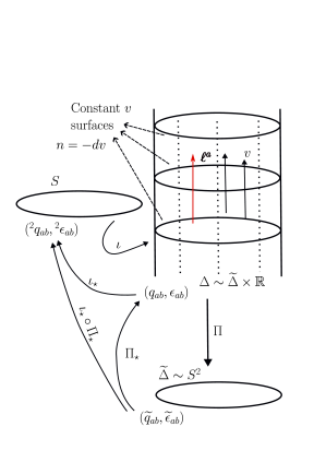
Figure 1: The projection map $\Pi$ and the foliation of the horizon. The NEH $\Delta$ is topologically $S^{2}\times\mathbb{R}$ and projects to the base-space $\widetilde{\Delta}$ of spherical topology. The fields $(\widetilde{q}_{ab},\widetilde{\omega}_{a})$ live on the base space and can be pulled back through $\Pi_{\star}$ to the fields $(q_{ab},\omega_{a})$ on $\Delta$. These are guaranteed to satisfy $\mathscr{L}_{\ell}q_{ab}=0$ and $\mathscr{L}_{\ell}\omega=0$. For a choice of affine parameter $v$ along the null-normal $\ell^{a}$ (satisfying $\ell^{a}\nabla_{a}v=1$), the constant $v$ surfaces yield a foliation of $\Delta$ which are shown as cross-sections in the figure. Each of these cross-sections can be considered as an embedding of a manifold $S$ (again with topology $S^{2}$) into $\Delta$. We can identify $S$ with $\widetilde{\Delta}$ in a natural way using the composition $\Pi\circ\iota:S\rightarrow\widetilde{\Delta}$. Thus, with a slight abuse of notation, we shall use the notation $\widetilde{q}_{ab}$ and $\widetilde{\epsilon}_{ab}$ instead of ${}^{2}q_{ab}$ and ${}^{2}\epsilon_{ab}$.

We can introduce a derivative operator $\mathscr{D}$ on a NEH $\Delta$. As mentioned before, the degeneracy of $q_{ab}$ implies that there are an infinite number of torsion-free derivative operators that are compatible with it. However, on an NEH, the property $\hbox{\lower 3.65973pt\hbox{${}_{\longleftarrow\!\!-\!\!-\!\!-\!\!-}$}}\kern-27.55544pt{\nabla_{(a}\ell_{b)}}=0$ can be used to construct a unique (torsion-free) derivative operator. It can be shown that this condition signifies that the space-time connection $\nabla$ induces a unique torsion-free derivative operator $\mathscr{D}$ on $\Delta$ which is compatible with $q_{ab}$ [43]; thus $\mathscr{D}_{a}=\hbox{\lower 3.65973pt\hbox{${}_{\longleftarrow}$}}\kern-12.91663pt{\nabla_{a}}$. We thus need to specify the pair $(q_{ab},\mathscr{D}_{a})$ to fully characterize the geometry of $\Delta$, and our strategy will be to strengthen the notion of a NEH by imposing restrictions on various components of $\mathscr{D}_{a}$.

Some of the various relevant geometric objects and manifolds are indicated in Fig. 1. This figure shows the different kinds of geometric objects in our problem, and it will be worthwhile to elaborate on these briefly; details may be found in [46]. Since $\Delta$ is a null surface, it is non-trivial to raise and lower indices and it is important to keep track of these. We can project $\Delta$ to a topological sphere (the “base-space” $\widetilde{\Delta}$) by identifying points on $\Delta$ connected by a null generator. We get in this way a natural projection $\Pi:\widetilde{\Delta}\times\mathbb{R}\rightarrow\widetilde{\Delta}$. It is straightforward to generalize $\widetilde{\Delta}$ to be a compact manifold without boundary, but we shall restrict ourselves to a sphere in this work. We equip $\widetilde{\Delta}$ with a Riemannian metric $\widetilde{q}_{ab}$ which gives us the derivative operator, volume element, and scalar curvature $\widetilde{\mathscr{D}}_{a}$, $\widetilde{\epsilon}_{ab}$ and $\widetilde{\mathscr{R}}$, respectively. We can pull-back these fields to $\Delta$ using the differential $\Pi_{\star}$ to obtain a degenerate metric $q_{ab}$ and a 2-form $\epsilon_{ab}$ on $\Delta$:

$$q_{ab}=\Pi_{\star}\widetilde{q}_{ab}\,,\quad\epsilon_{ab}=\Pi_{\star}\widetilde{\epsilon}_{ab}\,.$$ (4)

These are evidently seen to satisfy $\mathscr{L}_{\ell}q_{ab}=0=\mathscr{L}_{\ell}\epsilon_{ab}$, and $q_{ab}\ell^{b}=0=\epsilon_{ab}\ell^{b}$.

The foliation of the horizon requires a function $v$ whose level sets give the leaves of the foliation. We shall tie the null-normal to the foliation by $\ell^{a}\nabla_{a}v=1$ and $n_{a}=-\mathscr{D}_{a}v$ (so that $\ell\cdot n=-1$) is the 1-form orthogonal to the foliation. A given sphere of the foliation can be considered to be an embedding of a sphere $S$ into $\Delta$, i.e. $\iota:S\rightarrow\Delta$. This map allows us to pull-back various fields to $S$; in the literature one often uses the notation ${}^{2}q_{ab}=\iota_{\star}q_{ab}$ and ${}^{2}\epsilon_{ab}=\iota_{\star}\epsilon_{ab}$. To avoid notational clutter, we shall however generally not not use this notation, and we shall use instead $\widetilde{q}_{ab},\widetilde{\epsilon}_{ab}$. Thus, we shall use $\widetilde{q}_{ab}$ to refer to both the metric on a cross-section $S$ and also on the base-space $\widetilde{\Delta}$, and it shall be clear from the context which is meant. This discussion also makes clear that just as for the Kerr event horizon, any complete spherical cross-section of $\Delta$ has the same area. This area is a geometric invariant of $\Delta$, and we can talk sensibly about “the area $A$ of $\Delta$”, and its area radius $R=\sqrt{A/4\pi}$.

When embedded in a spacetime manifold, we can consider $n_{a}$ to be the pullback of a spacetime 1-form corresponding to a future-directed null vector $n^{a}$; this is the ingoing null normal to $\Delta$. Finally, we can complete $(\ell^{a},n^{a})$ to a null tetrad $(\ell^{a},n^{a},m^{a},\bar{m}^{a})$ by introducing a complex null vector $m^{a}$ tangent to the leaves of the foliation, such that $\ell\cdot m=n\cdot m=0$, and $m\cdot\bar{m}=1$. As we shall see, this tetrad can be extended to a neighborhood of $\Delta$ and tensor fields can be decomposed in terms of $(\ell^{a},n^{a},m^{a},\bar{m}^{a})$. This forms the basis of the Newman-Penrose formalism [72, 73, 74, 75]. which we will summarize it in Sec. III.1.

On a NEH, there is no canonical scaling of the null generators: $\ell^{a}$ and $f\ell^{a}$ (for any positive non-vanishing function $f$) are both perfectly acceptable. In the standard Schwarzschild/Kerr solutions, we have globally defined timelike and rotational Killing vectors available to us. For a Schwarzschild black hole, the timelike Killing vector is also a null generator of the horizon. Thus, for that solution, we get a preferred null generator by normalizing the timelike Killing vector to have unit norm at infinity. A similar strategy is also available in Kerr. This strategy is generically not viable because the spacetime in the vicinity of the isolated horizon will generally not be stationary; thus we will not have access to spatial infinity where the Killing vector could be normalized. As we shall see, it is nonetheless possible to single out a preferred class of null normals on an isolated horizon.

Two null normals $\ell^{a}$ and $\tilde{\ell}^{a}$ to an NEH $\Delta$ are said to belong to the same equivalence class $[\ell]$ if $\tilde{\ell}^{a}=c\ell^{a}$ for some positive constant $c$. Weakly isolated horizons are characterized by the property that, in addition to the metric $q_{ab}$, the connection component $\mathscr{D}_{a}\ell^{b}$ is also ‘time-independent’. From the properties of $\ell^{a}$ discussed above, it is easy to show that there must exist a connection 1-form $\omega_{a}^{(\ell)}$ associated with any given $\ell^{a}$ such that

$$\mathscr{D}_{a}\ell^{b}=\omega^{(\ell)}_{a}\ell^{b}\,.$$ (5)

The acceleration is given by $\kappa_{(\ell)}=\ell^{a}\omega^{(\ell)}_{a}$. It can be easily verified that when $\ell^{a}\rightarrow f\ell^{a}$, $\omega_{a}$ undergoes a gauge transformation:

$$\omega^{(f\ell)}_{a}=\omega^{(\ell)}_{a}+\mathscr{D}_{a}\ln f\,.$$ (6)

However, $\omega$ is invariant under constant rescalings, a fact which will be useful for our next definition.

Definition 2: The pair $(\Delta,[\ell])$ is said to constitute a weakly isolated horizon (WIH) provided $\Delta$ is an NEH and each null normal $\ell^{a}$ in $[\ell]$ satisfies

$$\mathscr{L}_{\ell}\omega_{a}=0\,.$$ (7)

On a weakly isolated horizon, since we are allowed only constant rescalings, $\omega_{a}$ is invariant and we can drop the reference to $\ell^{a}$ on $\omega^{(\ell)}$. A WIH does not represent a real physical restriction on a NEH. We can always choose the equivalence class $[\ell]$ on a NEH, but there is no unique choice [46]. In numerous applications, a WIH is sufficient and there is no need to impose any further restrictions. The laws of black hole mechanics can be shown to hold for WIHs [43, 45] and they are also sufficient for numerous applications in numerical relativity simulations of black holes for calculating mass, angular momentum and higher multipole moments (see e.g. [65, 66, 27]). The zeroth law will in fact be useful for us. This is the result that the surface gravity $\kappa_{(\ell)}=\omega_{a}\ell^{a}$ is constant on $\Delta$.

The condition $\mathscr{L}_{\ell}\omega_{a}=0$ can be written as

$$\left[\mathscr{L}_{\ell},\mathscr{D}\right]\ell^{a}=0\,.$$ (8)

This form makes more explicit that this is a restriction on $\mathscr{D}_{a}$. An obvious generalization of this condition would be to require that all components of $\mathscr{D}_{a}$ should be ‘time-independent’. This leads us to our third definition:

Definition 3: The pair $(\Delta,[\ell])$ is said to constitute an isolated horizon (IH) provided $\Delta$ is an NEH and each null normal $\ell^{a}$ in $[\ell]$ satisfies

$$\left[\mathscr{L}_{\ell},\mathscr{D}\right]=0\,.$$ (9)

If an equivalence class $[\ell]$ can be found that satisfies Eq. (9) then the NEH is said to admit an IH structure. We shall later summarize the steps required for finding an admissible $[\ell]$ on a NEH.

II.2 Mass, angular momentum and higher multipoles

To define the physical parameters of a black hole, and for the laws of back hole mechanics to hold on the horizon, it is sufficient to consider a WIH. Unlike other treatments of this topic where the basic variables of a black hole are mass and angular momentum and the area is a derived quantity, here it is more natural to begin with the area and angular momentum. We have already seen that the area $A$ (and correspondingly, the radius $R$) is a geometric invariant on a NEH. Expressions for angular momentum and mass are based on Hamiltonian calculations within a suitable phase space. Here the phase space consists of a spacetime with a WIH as an inner-boundary. It is possible to carry out the detailed calculation in either metric or connection variables [42, 43, 45, 68, 76, 77]. Angular momentum is the Hamiltonian which generates rotations, while energy is the generator of time translations. In the context of a diffeomorphism invariant theory like general relativity, the relevant Hamiltonians are all integrals over the boundary 2-surfaces which in our case, are cross-sections of a WIH. This allows a clear identification of the energy and angular momentum of an axisymmetric WIH. Let us consider a WIH in a vacuum spacetime with an axial symmetry $\varphi^{a}$, i.e.

$$\mathscr{L}_{\varphi}q_{ab}=0\,,\quad\mathscr{L}_{\varphi}\omega_{a}=0\,.$$ (10)

Then, the angular momentum is

$$J=-\frac{1}{8\pi}\oint_{S}\left(\varphi^{a}\omega_{a}\right)\widetilde{\epsilon}\,,$$ (11)

where $S$ is a cross-section of $\Delta$. It can be shown that any cross-section $S$ will yield the same value of $J$ and thus, just like the area, $J$ is a geometric invariant we can talk sensibly about the value of $J$ for an axisymmetric WIH.

Turning now to notions of energy, here we will need a suitable time translation Killing vector on $\Delta$. This is taken to be of the form $A\ell^{a}-\Omega\varphi^{a}$, where $A,\Omega$ are constant on a given WIH but vary over phase space. In particular $\Omega$ is the angular velocity. Hamiltonian considerations lead to an expression for the mass as

$$M=\frac{1}{2R}\sqrt{R^{4}+4J^{2}}\,.$$ (12)

Note that for a non-spinning black hole this reduces to the Schwarzschild expression $M=R/2$. The Hamiltonian analysis of [43, 45] also yields expressions for the surface gravity and angular velocity in terms of $(A,J)$ (in fact, the important point is that the analysis of [43, 45] shows that these quantities can depend only on $A$ and $J$). We shall need the expression for the surface gravity later:

$$\widetilde{\kappa}(A,J)=\frac{R^{4}-4J^{2}}{2R^{3}\sqrt{R^{4}+4J^{2}}},$$ (13)

This is the usual expression for surface gravity for a Kerr metric and for Schwarzschild this becomes $\widetilde{\kappa}=(2R)^{-1}=(4M)^{-1}$.

The expression for the angular momentum can also be expressed in terms of a Weyl tensor component. In terms of the null tetrad $(\ell^{a},n^{a},m^{a},\bar{m}^{a})$, the Weyl tensor can be decomposed into 5 complex scalar quantities denoted $\Psi_{0},\Psi_{1},\Psi_{2},\Psi_{3}$, and $\Psi_{4}$. These will be described more fully in Sec. III.1, but for now, we only need the expression for $\Psi_{2}$ in terms of the Weyl tensor $C_{abcd}$:

$$\Psi_{2}=C_{abcd}\ell^{a}m^{b}\bar{m}^{c}n^{d}\,.$$ (14)

We shall see that $\Psi_{2}$ is a geometric invariant on a WIH. Its real part yields the scalar curvature $\widetilde{\mathscr{R}}$ of $\widetilde{q}_{ab}$, and its imaginary part is related to the exterior derivative of $\omega_{a}$:

$$\widetilde{\mathscr{R}}=-4\textrm{Re}\left[\Psi_{2}\right]\,,\quad d\omega=2\mathrm{Im}\left[\Psi_{2}\right]\epsilon\,.$$ (15)

The angular momentum can then be rewritten as

$$J=-\frac{1}{4\pi}\oint_{S}\zeta\mathrm{Im}[\Psi_{2}]\,\widetilde{\epsilon}\,,$$ (16)

where $\zeta$ is a “potential” for the $\varphi^{a}$ in the following sense:

$$\varphi^{a}\widetilde{\epsilon}_{ab}=\partial_{b}\zeta\,,\quad\oint_{S}\zeta\,\widetilde{\epsilon}=0\,.$$ (17)

(For a Kerr black hole, in terms of the usual spherical coordinates, it turns out that $\zeta=\cos\theta$).

Beyond the mass and angular momentum, the geometry of a WIH can be expressed in terms of multipole moments. The basic idea is to express $\Psi_{2}$ as an infinite set of numbers by decomposing it in terms of spherical harmonics. However, which spherical coordinates should we use, and how can we compare two different calculations which might employ different coordinate systems? As shown in [18], on an axisymmetric WIH one can define a set of invariant coordinates and orthonormal spherical harmonics $Y^{m}_{\ell}$ which can be used to decompose $\Psi_{2}$. In this way, we get a set of mass and spin multipole moments associated with the real and imaginary parts of $\Psi_{2}$, respectively:

$$I_{\ell}+iL_{\ell}=-\oint\Psi_{2}\,Y^{0}_{\ell}(\zeta)\widetilde{\epsilon}\,.$$ (18)

The zeroth mass moment $I_{0}$ is a topological invariant: $I_{0}=\sqrt{\pi}$. Assuming there are no conical singularities, the mass-dipole moment vanishes $I_{1}=0$. Similarly, if $\omega$ has no singularities corresponding to a magnetic monopole, then $L_{0}=0$. From (16), we see also that $L_{1}$ is proportional to the angular momentum.

The importance of $\Psi_{2}$ for us resides in the fact that it also encodes tidal deformations. Thus, for a black hole with a binary companion, when its horizon is deformed due to the tidal field of its companion, this deformation is a perturbation of $\Psi_{2}$ and thus changes these multipole moments from their Kerr values. In astrophysical applications where tidally perturbed black holes are expected to be close to Kerr, we use the horizon area and $L_{1}$ to identify the Kerr parameters. These Kerr parameters identify uniquely all the higher moments, and any deviations from these Kerr values are to be interpreted as tidal perturbations of the horizon geometry.

Finally, we note that there are alternative definitions of multipole moments available in the literature. After all, different choices of spherical coordinates are possible, which lead to different spherical harmonics and thus to different multipole moments. One should thus be careful in interpreting the multipole moments and corresponding Love numbers. We mention in particular the multipole moments defined in [57] which exploits the conformal geometry of the horizon cross-sections.

II.3 Constraint equations on an isolated horizon

As discussed in the previous section, the geometry of $\Delta$ is completely specified by the degenerate metric $q_{ab}$, and the derivative operator $\mathscr{D}_{a}$. Since $q_{ab}\ell^{b}=0$, the “non-degenerate part” of $q_{ab}$ is simply $\widetilde{q}_{ab}$ constructed above. The information within $\mathscr{D}_{a}$ is conveniently written in terms of the ingoing null-normal $n_{a}$ to the horizon, which satisfies the normalization condition $\ell\cdot n=-1$. Starting from an initial cross-section $S_{0}$ and its normal $n_{a}$, we can extend this everywhere on $\Delta$ by requiring $\mathscr{L}_{\ell}n_{a}=0$ (and maintaining $\ell^{a}n_{a}=-1$).

We then introduce the tensor $S_{ab}$

$$S_{ab}=\mathscr{D}_{a}n_{b}\,.$$ (19)

Without loss of generality, we can take $\mathscr{D}_{[a}n_{b]}=0$ so that $S_{ab}$ is symmetric. It is easy to verify that $\omega_{a}=S_{ab}\ell^{b}$. The remaining information in $S_{ab}$ is thus obtained by projecting to the cross-section:

$$\widetilde{S}_{ab}=\widetilde{q}_{a}{}^{c}\widetilde{q}_{b}{}^{d}S_{cd}\,.$$ (20)

The trace and tracefree parts of $\widetilde{S}_{ab}$ yield respectively the expansion and shear of $n_{a}$. The complete characterization of $\Delta$ requires a specification of $\widetilde{S}_{ab}$ everywhere on $\Delta$. It can be shown that $\widetilde{S}_{ab}$ satisfies the following constraint equation [46]

$$\mathscr{L}_{\ell}\widetilde{S}_{ab}=-\kappa_{(\ell)}\widetilde{S}_{ab}+\mathscr{\widetilde{\mathscr{D}}}_{(a}\widetilde{\omega}_{b)}+\widetilde{\omega}_{a}\widetilde{\omega}_{b}-\frac{1}{2}\widetilde{\mathscr{R}}_{ab}\,.$$ (21)

Here $\widetilde{\mathscr{R}}_{ab}$ is the Ricci tensor on the cross-section calculated from the 2-metric $\widetilde{q}_{ab}$. Thus, by specifying $\widetilde{S}_{ab}$ on some initial cross-section, a solution of this constraint equation then yields $\widetilde{S}_{ab}$ everywhere on $\Delta$.

These geometric quantities and identities can be employed to choose a suitable equivalence class $[\ell^{a}]$ on a NEH and thereby find an admissible IH. As shown in [46], a suitable condition is to require that the expansion of $n^{a}$ is time-independent. Under this condition, one can choose an equivalence class $[\ell^{a}]$ if the following elliptic operator is invertible:

$$L:=\widetilde{\mathscr{D}}^{2}+2\widetilde{\omega}^{a}\widetilde{\mathscr{D}}_{a}+\widetilde{\mathscr{D}}^{a}\widetilde{\omega}_{a}+\widetilde{\omega}^{a}\widetilde{\omega}_{a}-\frac{1}{2}\widetilde{\mathscr{R}}\,.$$ (22)

It is interesting to note that the invertibility of a very similar operator appears in the stability analysis of marginally trapped surfaces [78, 79]. When the cross-section is taken to be a marginally trapped surface lying on a Cauchy surface, then the stability of the MOTS under deformations is shown to be equivalent to the invertibility of $L$.

Apart from the constraint equation Eq. (21), it turns out that there are additional constraints on $\Psi_{2}$ appearing due to the algebraic nature of the Weyl tensor. If one imposes constraints on the other Weyl tensor components, it turns out that the Bianchi identities restrict $\Psi_{2}$ as well. This is important for us because, as we have mentioned earlier, the geometric multipoles of an IH are determined by $\Psi_{2}$. Therefore, such constraints potentially limit the type of tidal perturbations that are allowed on an IH. As an example, it was shown in [80, 81, 82] that if the Weyl tensor is time dependent at $\Delta$ and is of Petrov type D, i.e. if we can find a frame in which $\Psi_{2}$ is the only non-vanishing Weyl tensor component on the horizon, then it cannot be specified freely but must satisfy

$$\eth\eth\Psi_{2}^{-1/3}=0\,.$$ (23)

Here $\eth$ is the spin-weighted angular derivative operator [83], which we will formally introduce in Sec. III.1 (for the action of the $\eth$ operator on the spin-weighted spherical harmonics see Appendix B). We will see that this condition implies that if we require non-trivial tidal perturbations, then $\Psi_{3}$ and/or $\Psi_{4}$ cannot vanish at the horizon. These components of the Weyl tensor indicate the presence of gravitational radiation at the horizon which is transverse to $\Delta$, i.e. not infalling into the black hole. This result shows that such radiation must be present for a tidally disturbed black hole. The Robinson-Trautman solutions [70, 71] furnish good examples of spacetimes with such transverse radiation in the vicinity of an IH; these solutions will be discussed in Sec. III.4.

III Constructing the near horizon spacetime

III.1 The Newman-Penrose formalism

With the intrinsic geometry of an isolated horizon understood, here we shall summarize the construction of the near horizon geometry. It will be convenient to work with the Newman-Penrose formalism. For this, as mentioned earlier, we complete the null normals $(\ell^{a},n^{a})$ to a null-tetrad $(\ell^{a},n^{a},m^{a},\bar{m}^{a})$ satisfying

$$\ell\cdot n=-1\,,m\cdot\bar{m}=1\,,$$ (24)

with all other inner products vanishing. The directional covariant derivatives along these basis vectors are denoted as

$$D:=\ell^{a}\nabla_{a}\,,\quad,\Delta:=n^{a}\nabla_{a}\,,\quad\delta:=m^{a}\nabla_{a}\,.$$ (25)

The connection is explicitly represented as a set of 12 complex functions known as the spin coefficients. These are typically represented in terms of the directional derivatives of the basis vectors:

$$D\ell =(\epsilon+\bar{\epsilon})\ell-\bar{\kappa}m-\kappa\bar{m}\,,$$ (26a)

$$Dn =-(\epsilon+\bar{\epsilon})n+\pi m+\bar{\pi}m\,,$$ (26b)

$$Dm =\bar{\pi}\ell-\kappa n+(\epsilon-\bar{\epsilon})m\,,$$ (26c)

$$\Delta\ell =(\gamma+\bar{\gamma})\ell-\bar{\tau}m-\tau\bar{m}\,,$$ (26d)

$$\Delta n =-(\gamma+\bar{\gamma})n+\nu m+\bar{\nu}\bar{m}\,,$$ (26e)

$$\Delta m =\bar{\nu}\ell-\tau n+(\gamma-\bar{\gamma})m\,,$$ (26f)

$$\delta\ell =(\bar{\alpha}+\beta)\ell-\bar{\rho}m-\sigma\bar{m}\,,$$ (26g)

$$\delta n =-(\bar{\alpha}+\beta)n+\mu m+\bar{\lambda}\bar{m}\,,$$ (26h)

$$\delta m =\bar{\lambda}\ell-\sigma n+(\beta-\bar{\alpha})m\,,$$ (26i)

$$\bar{\delta}m =\bar{\mu}\ell-\rho n+(\alpha-\bar{\beta})m\,.$$ (26j)

A technical benefit of tetrad formalisms is that the covariant derivatives (here the spin coefficients) can be calculated using only exterior derivatives. This is useful in practical calculations because, given a metric, the calculation of the spin coefficients require a fewer number of derivatives and no Christoffel symbols are required. It can be shown that the exterior derivatives of the basis 1-forms are:

$$d\ell =(\epsilon+\bar{\epsilon})\ell\wedge n+[\bar{\tau}-(\alpha+\bar{\beta})]\ell\wedge m+[\tau-(\bar{\alpha}+\beta)]\ell\wedge\bar{m}+\bar{\kappa}n\wedge m+\kappa n\wedge\bar{m}+(\bar{\rho}-\rho)m\wedge\bar{m}\,,$$ (27a)

$$dn =(\gamma+\bar{\gamma})\ell\wedge n-\nu\ell\wedge m-\bar{\nu}\ell\wedge\bar{m}-[\pi-(\alpha+\bar{\beta})]n\wedge m-[\bar{\pi}-(\bar{\alpha}+\beta)]n\wedge\bar{m}+(\bar{\mu}-\mu)m\wedge\bar{m}\,,$$ (27b)

$$dm =(\tau+\bar{\pi})\ell\wedge n-[\bar{\mu}+(\gamma-\bar{\gamma})]\ell\wedge m+\bar{\lambda}\ell\wedge\bar{m}+[\rho-(\epsilon-\bar{\epsilon})]n\wedge m+\sigma n\wedge\bar{m}+(\bar{\alpha}-\beta)m\wedge\bar{m}\,.$$ (27c)

Some important spin coefficients for us are: the real parts of $\rho$ and $\mu$ are the expansion of $\ell$ and $n$ respectively; the imaginary parts yield the twist; $\sigma$ and $\lambda$ are the shears of $\ell$ and $n$ respectively; the vanishing of $\kappa$ and $\nu$ implies that $\ell$ and $n$ are respectively geodesic; $\epsilon+\bar{\epsilon}$ and $\gamma+\bar{\gamma}$ are respectively the accelerations of $\ell$ and $n$, $\alpha-\bar{\beta}$ yields the connection in the $m$-$\bar{m}$ plane and thus the curvature of the manifold spanned by $m$-$\bar{m}$.

Since the null tetrad is typically not a coordinate basis, the above definitions of the spin coefficients lead to non-trivial commutation relations:

$$(\Delta D-D\Delta)f =(\epsilon+\bar{\epsilon})\Delta f+(\gamma+\bar{\gamma})Df-(\bar{\tau}+\pi)\delta f-(\tau+\bar{\pi})\bar{\delta}f\,,$$ (28a)

$$(\delta D-D\delta)f =(\bar{\alpha}+\beta-\bar{\pi})Df+\kappa\Delta f-(\bar{\rho}+\epsilon-\bar{\epsilon})\delta f-\sigma\bar{\delta}f\,,$$ (28b)

$$(\delta\Delta-\Delta\delta)f =-\bar{\nu}Df+(\tau-\bar{\alpha}-\beta)\Delta f+(\mu-\gamma+\bar{\gamma})\delta f+\bar{\lambda}\bar{\delta}f\,,$$ (28c)

$$(\bar{\delta}\delta-\delta\bar{\delta})f =(\bar{\mu}-\mu)Df+(\bar{\rho}-\rho)\Delta f+(\alpha-\bar{\beta})\delta f-(\bar{\alpha}-\beta)\bar{\delta}f\,.$$ (28d)

The Weyl tensor $C_{abcd}$ breaks down into 5 complex scalars

$$\Psi_{0} =C_{abcd}\ell^{a}m^{b}\ell^{c}m^{d}\,,\quad\Psi_{1}=C_{abcd}\ell^{a}m^{b}\ell^{c}n^{d}\,,$$ (29a)

$$\Psi_{2} =C_{abcd}\ell^{a}m^{b}\bar{m}^{c}n^{d}\,,\quad\Psi_{3}=C_{abcd}\ell^{a}n^{b}\bar{m}^{c}n^{d}\,,$$ (29b)

$$\Psi_{4} =C_{abcd}\bar{m}^{a}n^{b}\bar{m}^{c}n^{d}\,.$$ (29c)

Similar decompositions apply for the Ricci tensor or Maxwell fields, but since we deal with vacuum spacetimes in this paper, we do not need these here.

The relation between the spin coefficients and the curvature components lead to the so-called Newman-Penrose field equations which are a set of 16 complex first order differential equations. The Bianchi identities, $\nabla_{[a}R_{bc]de}=0$, are written explicitly as 8 complex equations involving both the Weyl and Ricci tensor components, and 3 real equations involving only Ricci tensor components. See [73, 74, 75] for the full set of field equations and Bianchi identities (but beware that they use slightly different conventions such as the sign for the metric signature and normalization of the null tetrad, leading to possible minus sign changes).

It will also be useful to use the notion of spin weights and the $\eth$ operator for derivatives in the $m$-$\bar{m}$ plane (which will be angular derivatives in our case). A tensor $X$ projected on the $m$-$\bar{m}$ plane is said to have spin weight $s$ if under a spin rotation $m\rightarrow e^{i\psi}m$, it transforms as $X\rightarrow e^{is\psi}X$. Thus, $m^{a}$ itself has spin weight $+1$ while $\bar{m}^{a}$ has weight $-1$. For instance, the scalar $X=m^{a_{1}}\cdots m^{a_{p}}\bar{m}^{b_{1}}\cdots\bar{m}^{b_{q}}X_{{a_{1}}\cdots{b_{q}}}$ has spin weight $s=p-q$ and the Weyl tensor component $\Psi_{k}$ has spin weight $2-k$.

The $\eth$ and $\bar{\eth}$ operators are defined as

$$\eth X=m^{a_{1}}\cdots m^{a_{p}}\bar{m}^{b_{1}}\cdots\bar{m}^{b_{q}}\delta X_{{a_{1}}\cdots{b_{q}}}\,,$$ (30)

$$\bar{\eth}X=m^{a_{1}}\cdots m^{a_{p}}\bar{m}^{b_{1}}\cdots\bar{m}^{b_{q}}\bar{\delta}X_{{a_{1}}\cdots{b_{q}}}\,.$$ (31)

From Eqs. (26i) and (26j), after projecting on to the $m$-$\bar{m}$ plane, we get

$$\delta m^{a}=(\beta-\bar{\alpha})m^{a}\,,\qquad\bar{\delta}{m}^{a}=(\alpha-\bar{\beta})m^{a}\,.$$ (32)

A short calculation shows that

$$\eth X=\delta X+s(\bar{\alpha}-\beta)X\,,\qquad\bar{\eth}X=\bar{\delta}X-s(\alpha-\bar{\beta})X\,.$$ (33)

It is clear that $\eth$ and $\bar{\eth}$ act as spin raising and lowering operators. See [83] for further properties of the $\eth$ operator and its connection to representations of the rotation group.

The transformations of the null tetrad which preserve their inner product are

Boosts and Spin Rotations

$$l\rightarrow Al\,,\quad n\rightarrow A^{-1}n\,,\quad m\rightarrow e^{i\theta}m\,,$$ (34)

Null rotations

$$\ell\rightarrow\ell\,,\quad m\rightarrow m+a\ell\,,\quad n\rightarrow n+\bar{a}m+a\bar{m}+|a|^{2}\ell\,,$$ (35)

and the null rotations around $n$ (obtained by interchanging $\ell$ and $n$ in Eq. (35)).

We refer to [73, 74, 75] for a more complete discussion.

III.2 A general construction of the near horizon spacetime

The construction of the near horizon geometry follows, in principle, the same philosophy as the standard 3+1 decomposition: we prescribe initial data on certain hypersurfaces and use the Einstein equations to obtain the spacetime metric in a neighborhood. The difference is that instead of specifying data on a spatial hypersurface, we use a characteristic initial value problem and prescribe data on a pair of transverse null hypersurfaces [84, 50]. We refer here also to the seminal work by Bondi and collaborators on constructing the spacetime near null infinity [85] following a similar procedure.

In the characteristic formalism, the field equations (i.e. the Einstein equations and the Bianchi identities) are written as first-order quasi-linear equations of the form

$$\sum_{J=1}^{N}A^{a}_{IJ}(x,\psi)\partial_{a}\psi_{J}+F_{I}(x,\psi)=0\,.$$ (36)

Here $x^{a}$ are coordinates on a manifold, and we have $N$ dependent variables $\psi_{I}$. In the usual Cauchy problem, we specify $\psi_{I}$ at some initial time, and solve these equations to obtain $\psi_{I}$ for later times. Alternatively, within the characteristic formulation, we have a pair of null surfaces $\mathscr{N}_{0}$ and $\mathscr{N}_{1}$ whose intersection is a co-dimension-2 spacelike surface $S$. It turns out to be possible to specify appropriate data on the null surfaces and on $S$ such that the above system of equations is well-posed and has a unique solution, at least locally near $S$. We briefly summarize this construction in our present case.

One of the null surfaces will be the isolated horizon $\Delta$, while the other null surface $\mathscr{N}$ is generated by past-directed null geodesics emanating from a cross-section of $\Delta$ as shown in Fig. 2. This construction was first proposed in [51, 44] and further elaborated upon in [54, 52, 86]. We start with the past-directed null vector $-n^{a}$ at the horizon obtained from a particular cross-section $S_{0}$. Integrating the geodesic equation (till the conjugate point) gives us the null geodesics generated by $-n^{a}$, and thus yields a null surface $\mathscr{N}$ generated from $S_{0}$. The spacetime metric is calculated in a characteristic formulation by prescribing initial data on the null surfaces $\mathscr{N}$ and $\Delta$. The data on $\mathscr{N}$ is the Weyl tensor component $\Psi_{4}$ while the data on $\Delta$ consist of the geometric information required for an IH, i.e. $(q_{ab},\mathscr{D},[\ell^{a}])$. If we have coordinates $(v,\theta,\phi)$ on $\Delta$ such that $S_{0}$ is a surface of constant $v$ and $(\theta,\phi)$ are coordinates on $S_{0}$, and $r$ is the affine parameter along $-n^{a}$, then this construction yields a coordinate system $(v,r,\theta,\phi)$ in a neighborhood of $\Delta$. For technical convenience, instead of real angular coordinates $(\theta,\phi)$, we shall work on the stereographic plane with complex coordinates $(z,\bar{z})$.

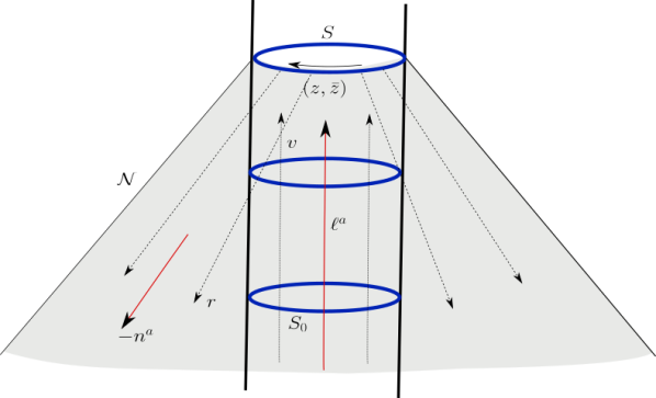
Figure 2: The characteristic initial value problem for constructing the near horizon geometry. Here $\Delta$ is the horizon whose geometry is shown in Fig. 1. The null surface $\mathscr{N}$ is generated by past-directed null geodesics starting from a cross-section $S$ with coordinates $(z,\bar{z})$. The affine parameter along the geodesics is $r$, and the null vector is $n^{a}\partial_{a}=-\partial_{r}$. The spacetime metric is constructed starting with suitable data on $\Delta$, $\mathscr{N}$ and $S$.

The above construction implies that we can choose

$$n_{a}=-\partial_{a}v\qquad\textrm{and}\qquad n^{a}\nabla_{a}:=\Delta=-\frac{\partial}{\partial r}\,.$$ (37)

To satisfy the inner product relations $\ell^{a}n_{a}=-1$ and $m^{a}n_{a}=0$, the other basis vectors must be of the form:

$$\ell^{a}\nabla_{a} :=D=\frac{\partial}{\partial v}+U\frac{\partial}{\partial r}+X\frac{\partial}{\partial z}+\bar{X}\frac{\partial}{\partial\bar{z}}\,,$$ (38a)

$$m^{a}\nabla_{a} :=\delta=\Omega\frac{\partial}{\partial r}+\xi_{1}\frac{\partial}{\partial z}+\xi_{2}\frac{\partial}{\partial\bar{z}}\,.$$ (38b)

The frame function $U$ is real while $X,\Omega,\xi_{i}$ are complex. We wish to now specialize to the case when $\ell^{a}$ is a null normal of $\Delta$ so that the null tetrad is adapted to the horizon. Since $\partial_{v}$ is tangent to the null generators of $\Delta$, this clearly requires that $U,X^{i}$ must vanish on the horizon. Similarly, we want $m^{a}$ to be tangent to the spheres $S_{v}$ at the horizon, so $\Omega$ should also vanish on $\Delta$.

Since $n^{a}$ is an affinely parameterized geodesic, and $\ell$ and $m$ are parallel propagated along $n^{a}$, we have $\Delta n=\Delta\ell=\Delta m=0$. From Eqs. (26d), (26e) and (26f), this leads to

$$\gamma=\tau=\nu=0\,.$$ (39)

We first impose these conditions to the commutation relations in Eqs. (28). Then, setting $f=v$ in those equations leads to

$$\pi=\alpha+\bar{\beta}\,,\quad\mu=\bar{\mu}\,.$$ (40)

These must hold throughout the region where the coordinate system is valid.

The rest of the discussion can be separated into three parts: i) equations which involve the time derivatives along $\ell^{a}$ and include a description of the horizon geometry, ii) the radial derivatives along $n^{a}$ which propagate geometric information away from $\Delta$, and iii) equations which exclusively involve angular derivatives and yield the “shape” of the 2-sphere cross-sections. At the horizon, since the expansion, shear, and twist of $\ell^{a}$ vanish, we have:

$$\rho\triangleq 0,\quad\kappa\triangleq 0\,,\quad\sigma\triangleq 0\,.$$ (41)

(Equations which hold only on $\Delta$ are indicated by ‘$\triangleq$’ instead of the usual ‘$=$’). These three conditions at the horizon further imply

$$\Psi_{0}\triangleq 0\,,\quad\Psi_{1}\triangleq 0\,.$$ (42)

These two equations can be interpreted as the absence of ingoing transverse and longitudinal radiation at the horizon. Further, we can require $m^{a}$ to be Lie-dragged along $\ell^{a}$ so that $\mathscr{L}_{\ell}m^{a}=0$. This leads to

$$\epsilon-\bar{\epsilon}\triangleq 0\,.$$ (43)

In terms of the Newman-Penrose spin coefficients, the connection 1-form $\omega_{a}$ is written as

$$\omega_{a}=-n_{b}\nabla_{a}\ell^{b}={-}(\epsilon+\bar{\epsilon})n_{a}+\pi m_{a}+\bar{\pi}\bar{m}_{a}\,.$$ (44)

Thus, $\Delta$ will be a WIH if we choose

$$\tilde{\kappa}_{(\ell)}\triangleq\epsilon+\bar{\epsilon}\triangleq\textrm{constant}\,,\quad D\pi\triangleq 0\,.$$ (45)

The first of the above is just the zeroth law of black hole mechanics stating that the surface gravity is constant. Notice that Eqs. (41), (42) and (45) further imply that

$$D\Psi_{2}\triangleq 0\,,\quad Da\triangleq 0\,,$$ (46)

where $a=\alpha-\bar{\beta}$ is the connection compatible with $\widetilde{q}_{ab}$. This last equation specifies that the geometry of $\tilde{\Delta}$ is constant in time.

With the above conditions on the spin coefficients at hand, we now impose them in the commutator relations, the field equations, and the Bianchi identities. The functions $U,X^{i},\Omega,\xi^{i}$ are determined by the commutation relations (28) by substituting, in turn, $r$ and $x^{i}$ for $f$, and imposing Eqs. (39) and (40) on the spin coefficients. First, the radial derivatives for the coefficients of the tetrad are

$$\Delta U =-(\epsilon+\bar{\epsilon})-\pi\Omega-\bar{\pi}\bar{\Omega}\,,$$ (47a)

$$\Delta X^{i} =-\pi\xi^{i}-\bar{\pi}\bar{\xi}^{i}\,,$$ (47b)

$$\Delta\Omega =-\bar{\pi}-\mu\Omega-\bar{\lambda}\bar{\Omega}\,,$$ (47c)

$$\Delta\xi^{i} =-\mu\xi^{i}-\bar{\lambda}\bar{\xi}^{i}\,,$$ (47d)

while their propagation equations along $v$ are

$$D\Omega-\delta U =\kappa+\rho\Omega+\sigma\bar{\Omega}\,,$$ (48a)

$$D\xi^{i}-\delta X^{i} =(\bar{\rho}+\epsilon-\bar{\epsilon})\xi^{i}+\sigma\bar{\xi}^{i}\,.$$ (48b)

Let us now turn to the field equations. After imposing Eqs. (39) and (40) on the spin coefficients and ignoring matter terms, the field equations involving radial derivatives are:

$$\Delta\lambda =-2\lambda\mu-\Psi_{4}\,,$$ (49a)

$$\Delta\mu =-\mu^{2}-|\lambda|^{2}\,,$$ (49b)

$$\Delta\rho =-\mu\rho-\sigma\lambda-\Psi_{2}\,,$$ (49c)

$$\Delta\sigma =-\mu\sigma-\bar{\lambda}\rho\,.$$ (49d)

$$\Delta\kappa =-\bar{\pi}\rho-\pi\sigma-\Psi_{1}\,,$$ (49e)

$$\Delta\epsilon =-\bar{\pi}\alpha-\pi\beta-\Psi_{2}\,,$$ (49f)

$$\Delta\pi =-\pi\mu-\bar{\pi}\lambda-\Psi_{3}\,,$$ (49g)

$$\Delta\beta =-\mu\beta-\alpha\bar{\lambda}\,,$$ (49h)

$$\Delta\alpha =-\beta\lambda-\mu\alpha-\Psi_{3}\,.$$ (49i)

The time evolution equations become:

$$D\rho-\bar{\delta}\kappa =\rho^{2}+|\sigma|^{2}+(\epsilon+\bar{\epsilon})\rho-2\alpha\kappa\,,$$ (50a)

$$D\sigma-\delta\kappa =(\rho+\bar{\rho}+\epsilon+\bar{\epsilon})\sigma-2\beta\kappa+\Psi_{0}\,,$$ (50b)

$$D\alpha-\bar{\delta}\epsilon =(\rho+\bar{\epsilon}-2\epsilon)\alpha+\beta\bar{\sigma}-\bar{\beta}\epsilon-\kappa\lambda+(\epsilon+\rho)\pi\,,$$ (50c)

$$D\beta-\delta\epsilon =(\alpha+\pi)\sigma+(\bar{\rho}-\bar{\epsilon})\beta-\mu\kappa-(\bar{\alpha}-\bar{\pi})\epsilon+\Psi_{1}\,,$$ (50d)

$$D\lambda-\bar{\delta}\pi =(\rho-2\epsilon)\lambda+\bar{\sigma}\mu+2\alpha\pi\,,$$ (50e)

$$D\mu-\delta\pi =(\bar{\rho}-\epsilon-\bar{\epsilon})\mu+\sigma\lambda+2\beta\pi+\Psi_{2}\,.$$ (50f)

The angular field equations are:

$$\delta\rho-\bar{\delta}\sigma =\bar{\pi}\rho-(3\alpha-\bar{\beta})\sigma-\Psi_{1}\,,$$ (51a)

$$\delta\alpha-\bar{\delta}\beta =\mu\rho-\lambda\sigma+|\alpha|^{2}+|\beta|^{2}-2\alpha\beta-\Psi_{2}\,,$$ (51b)

$$\delta\lambda-\bar{\delta}\mu =\pi\mu+(\bar{\alpha}-3\beta)\lambda-\Psi_{3}\,.$$ (51c)

Finally, we have the Bianchi identities which, in the NP formalism, are written as a set of nine complex and two real equations; in the absence of matter, only 8 complex equations survive. The radial Bianchi identities are reduced to:

$$\Delta\Psi_{0}-\delta\Psi_{1} =-\mu\Psi_{0}-2\beta\Psi_{1}+3\sigma\Psi_{2}\,,$$ (52a)

$$\Delta\Psi_{1}-\delta\Psi_{2} =-2\mu\Psi_{1}+2\sigma\Psi_{3}\,,$$ (52b)

$$\Delta\Psi_{2}-\delta\Psi_{3} =-3\mu\Psi_{2}+2\beta\Psi_{3}+\sigma\Psi_{4}\,,$$ (52c)

$$\Delta\Psi_{3}-\delta\Psi_{4} =-4\mu\Psi_{3}+4\beta\Psi_{4}\,.$$ (52d)

Note that there is no equation for the radial derivative of $\Psi_{4}$. Among all the fields that we are solving for, this is in fact the only one for which this happens. This means that $\Psi_{4}$ (in this case, its radial derivatives) is the free data that must be specified on the null cone $\mathscr{N}_{0}$ originating from $S_{0}$. Notice that if the spacetime is algebraically special, $\Psi_{4}$ might satisfy further constraints, which need to be accounted for in the previous statement. For instance, for type $D$ spacetimes $\Psi_{4}$ (and its radial derivatives) are related to $\Psi_{2}$ and $\Psi_{3}$ through $2\Psi_{2}\Psi_{4}=3\Psi_{3}^{2}$ [80].

Finally, we have the components of the Bianchi equations for evolution of the Weyl tensor components:

$$D\Psi_{1}-\bar{\delta}\Psi_{0} =(\pi-4\alpha)\Psi_{0}+2(2\rho+\epsilon)\Psi_{1}-3\kappa\Psi_{2}\,,$$ (53a)

$$D\Psi_{2}-\bar{\delta}\Psi_{1} =-\lambda\Psi_{0}+2(\pi-\alpha)\Psi_{1}+3\rho\Psi_{2}-2\kappa\Psi_{3}\,,$$ (53b)

$$D\Psi_{3}-\bar{\delta}\Psi_{2} =-2\lambda\Psi_{1}+3\pi\Psi_{2}+2(\rho-\epsilon)\Psi_{3}-\kappa\Psi_{4}\,,$$ (53c)

$$D\Psi_{4}-\bar{\delta}\Psi_{3} =-3\lambda\Psi_{2}+2(\alpha+2\pi)\Psi_{3}+(\rho-4\epsilon)\Psi_{4}\,.$$ (53d)

Before proceeding to apply the above equations for a tidally distorted black hole, it will be instructive to look at two illustrative examples.

III.3 Example 1: Constructing the Schwarzschild spacetime

The reader will be familiar with the Schwarzschild metric of mass $M$ in ingoing Eddington-Finkelstein coordinates $(v,\mathfrak{r},z,\bar{z})$. Here we distinguish between the radial coordinate $r$ defined previously, which vanishes at the horizon, and the coordinate $\mathfrak{r}$, which is the usual Schwarzschild radial coordinate (at the horizon, $\mathfrak{r}=2M$):

$$ds^{2}=-f(\mathfrak{r})dv^{2}+2dv\,d\mathfrak{r}+\frac{2\mathfrak{r}^{2}}{P_{0}^{2}}dz\,d\bar{z}\,.$$ (54)

Here, as usual

$$f=1-\frac{2M}{\mathfrak{r}}\,.$$ (55)

Instead of the usual spherical coordinates, let us use complex coordinates $z=e^{i\phi}\cot{\frac{\theta}{2}}$. The expressions for the stereographic projection yield

$$P_{0}=\frac{1}{\sqrt{2}}(1+z\bar{z})\,.$$ (56)

Starting with just the data on the horizon, i.e. a spherically symmetric horizon, taking $\mathscr{N}$ to be a constant-$v$ surface, and setting $\Psi_{4}=0$ everywhere on $\mathscr{N}$, can we reconstruct the Schwarzschild metric? In particular, we have the usual null tetrad and basis 1-forms:

$$\ell^{a}\nabla_{a} =\partial_{v}+\frac{f}{2}\partial_{\mathfrak{r}}\,,\quad\ell_{a}=-\frac{f}{2}\partial_{a}v+\partial_{a}\mathfrak{r}\,,$$ (57a)

$$n^{a}\nabla_{a} =-\partial_{\mathfrak{r}}\,,\quad n_{a}=-\partial_{a}v\,,$$ (57b)

$$m^{a}\nabla_{a} =\frac{P}{\mathfrak{r}}\partial_{z}\,,\quad m_{a}=\frac{\mathfrak{r}}{P}\partial_{a}\bar{z}\,.$$ (57c)

It is straightforward to calculate the spin coefficients everywhere. But we want to instead just start with the spin coefficients at the horizon and recover their values everywhere following the construction outlined in the previous section.

This is in fact straightforward and instructive and we shall see in fact the resulting spacetime is asymptotically flat as it should be. We begin with the Weyl tensor components. We shall first assume that the metric is type D at the horizon, i.e.

$$\Psi_{0}\triangleq\Psi_{1}\triangleq\Psi_{3}\triangleq\Psi_{4}\triangleq 0\,.$$ (58)

We shall assume further that $\Psi_{2}$ is spherically symmetric so that the constraint of Eq. (23) is satisfied. Moreover, let us take the simplest choice of $\Psi_{4}=0$ on the transverse null surface $\mathscr{N}$. Next, choose the sphere $S_{0}=\mathscr{N}\cap\Delta$ to be spherically symmetric, in the sense that the expansion of $n_{a}$, i.e. $\mu$, is constant on $S_{0}$ and its shear, $\lambda\triangleq 0$.

The choice of $\Psi_{2}$ determines the horizon source multipole moments, and in this case we just have a mass monopole. First we note that if $\Psi_{2}$ is constant, it must be real because from Eq. (15)

$$\oint_{S_{0}}\mathrm{Im}{\Psi_{2}}\,\widetilde{\epsilon}=\oint_{S_{0}}d\omega=0\,.$$ (59)

On the other hand, if $\mathrm{Im}{\Psi_{2}}$ is constant then the above equation shows that it must vanish. Similarly, from Eq. (16) the angular momentum $J$ must also vanish, and thus from Eq. (12), the horizon mass is $M=R/2$.

The real part $\rm{\Psi_{2}}$ is determined by the topology of $S_{0}$ and the Gauss-Bonnet theorem. Since $\mathscr{R}=-4\mathrm{Re}{\Psi_{2}}$:

$$8\pi = \oint_{S_{0}}\mathscr{R}\widetilde{\epsilon}=-4\mathrm{Re}{\Psi_{2}}A\,,$$ (60)

$$\implies \Psi_{2}=-\frac{2\pi}{A}=-\frac{1}{2R^{2}}=-\frac{1}{8M^{2}}\,.$$ (61)

We can now in fact determine the constant value of $\mu$ on $\Delta$. Use the last of the evolution equations Eqs. (50) on $\Delta$, use $\kappa=0$ and impose $D\mu=0$ to obtain

$$\widetilde{\kappa}_{(\ell)}\mu=\Psi_{2}\,.$$ (62)

Using the canonical value $\widetilde{\kappa}$ (see the discussion around Eq. (13)), we conclude that $\mu\triangleq-1/(2M)$.

To obtain the Schwarzschild metric in the usual coordinates, let us take the radial coordinate such that $\mathfrak{r}=2M$ at the horizon. We begin with the first two radial equations from Eqs. (49) for the shear and expansion on $n^{a}$:

$$\Delta\lambda =-2\lambda\mu\implies\Delta(\lambda\bar{\lambda})=-4\mu|\lambda|^{2}\,.$$ (63a)

$$\Delta\mu =-\mu^{2}-|\lambda|^{2}\,.$$ (63b)

Note that $\Delta$ is $-\partial/\partial\mathfrak{r}$. At the horizon, we have $\lambda=0$, and therefore the first equation yields

$$|\lambda|^{2}=|\lambda_{0}|^{2}\exp\left(\int_{2M}^{\mathfrak{r}}4\mu\,d\mathfrak{r}\right)\,.$$ (64)

We conclude immediately that $\lambda=0$ everywhere if $\lambda_{0}=0$, as is the case given that $\lambda\triangleq 0$. Substituting this into the equation for $\mu$ yields

$$\frac{\mathrm{d}\mu}{\mathrm{d}\mathfrak{r}}=\mu^{2}\implies\frac{1}{\mu_{0}}-\frac{1}{\mu}=\mathfrak{r}-2M\,.$$ (65)

Since $\mu_{0}=-1/(2M)$, we find the solution everywhere on $\mathscr{N}$:

$$\mu=-\frac{1}{\mathfrak{r}}\,,$$ (66)

as it should be. With the solution for $\mu,\lambda$ at hand, and using $\sigma\triangleq 0$, the fourth radial equation from Eqs. (49) yields the solution $\sigma=0$ everywhere on $\mathscr{N}$.

Proceeding similarly, we now consider the radial Bianchi identities Eqs. (52) starting from the last to the first. The above boundary conditions on the Weyl tensor are sufficient to determine it everywhere on $\mathscr{N}$. With $\Psi_{4}=0$, the last of Eqs. (52) becomes

$$\Delta\Psi_{3}=-4\mu\Psi_{3}\implies\frac{\mathrm{d}\ln\Psi_{3}}{\mathrm{d}\mathfrak{r}}=4\mu\,.$$ (67)

This has the solution

$$\Psi_{3}(\mathfrak{r})=\Psi_{3}(\mathfrak{r}=2M)\exp\left(\int_{2M}^{\mathfrak{r}}4\mu\,\mathrm{d}\mathfrak{r}\right)\,.$$ (68)

The boundary condition $\Psi_{3}(\mathfrak{r}=2M)=0$ then implies that $\Psi_{3}(\mathfrak{r})=0$ everywhere on $\mathscr{N}$. The third radial Bianchi identity yields

$$\frac{\mathrm{d}\Psi_{2}}{\mathrm{d}\mathfrak{r}}=3\mu\Psi_{2}\,.$$ (69)

Using the solution $\mu=-1/\mathfrak{r}$ derived above, we get

$$\frac{\mathrm{d}\ln\Psi_{2}}{\mathrm{d}\mathfrak{r}}+\frac{3}{\mathfrak{r}}=0\implies\Psi_{2}\mathfrak{r}^{3}=\textrm{constant}\,.$$ (70)

Using the boundary condition Eq. (61) yields the solution

$$\Psi_{2}=-\frac{M}{\mathfrak{r}^{3}}\,.$$ (71)

This is, again, as expected from the full Schwarzschild solution. Finally, the first two Bianchi identities (and the solution $\sigma=0$) give $\Psi_{0}(\mathfrak{r})=\Psi_{1}(\mathfrak{r})=0$ everywhere on $\mathscr{N}$.

We can now proceed with the remaining radial equations in Eqs. (49), which all involve the Weyl tensor components. We conclude straightforwardly that $\pi=0$ which in turn gives $\kappa=0$. For $\epsilon$ and $\rho$ (with the boundary condition $\epsilon\triangleq 1/8M$ and $\rho\triangleq 0$), we get:

$$\Delta\epsilon = \frac{M}{\mathfrak{r}^{3}}\implies\epsilon(\mathfrak{r})=\frac{M}{2\mathfrak{r}^{2}}\,,$$ (72)

$$\Delta\rho = \frac{\rho}{\mathfrak{r}}+\frac{M}{\mathfrak{r}^{3}}\implies\rho(\mathfrak{r})=-\frac{1}{2\mathfrak{r}}\left(1-\frac{2M}{\mathfrak{r}}\right)\,.$$ (73)

We are finally left with $\alpha$ and $\beta$. These are related to the “shape” of the cross-section $S_{0}$ and the intrinsic 2-dimensional Ricci scalar $\widetilde{R}$. These will depend on the angular coordinates $(z,\bar{z})$. From Eq. (40) and $\pi=0$ we get $\alpha+\bar{\beta}=0$. The combination $\alpha-\bar{\beta}$ is determined just by angular derivatives and can be obtained from the 2-metric on $S_{0}$. Let us denote $a=\alpha-\bar{\beta}$. From the third of Eqs. (27), we have

$$a\triangleq\frac{\partial_{\bar{z}}P}{2M}\,,$$ (74)

where the stereographic function $P$ is defined in Eq. (56). This is the boundary conditions for the radial equations involving $\beta$ and $\alpha$. From the radial equations:

$$\Delta a=-\mu a=\frac{a}{\mathfrak{r}}\implies a(\mathfrak{r})=\frac{\partial_{\bar{z}}P}{\mathfrak{r}}\,.$$ (75)

Finally, since the Weyl tensor, along with $\mu,\lambda,\sigma$ are all time-independent on $\Delta$, the above analysis can be repeated on all the null surfaces starting from other spherically symmetric sections of $\Delta$. Thus, the expressions obtained above for the spin coefficients and Weyl tensor components are valid everywhere outside the horizon for all $v$. The metric itself is obtained by integrating the radial equations for the frame functions, i.e. Eqs. (47) and then combining the tetrad to obtain the metric. We leave this to the reader to verify that we do indeed obtain the Schwarzschild null tetrad given in Eqs. (57), and thus the Schwarzschild metric in ingoing Eddington-Finkelstein coordinates.

This concludes our derivation of the Schwarzschild solution using the characteristic initial value problem. This might seem to be a rather convoluted derivation of a simple and well-known metric. Nevertheless it illustrates the general procedure and clarifies the role played by the different quantities and equations (for this reason we have not spared any of the details). The payoff has been a very detailed understanding of the spacetime with explicit expressions for the curvature, connection (and, of course, also the metric if desired). These features will hold in more general physical situations as well. All aspects of the classical isolated horizon formalism are seen to be essential: a) The Hamiltonian calculations gave us appropriate values for mass and surface gravity, b) The geometric constraints on the isolated horizon needed to be satisfied in accordance with the algebraic properties of the Weyl tensor, c) The multipole moments yielded $\Psi_{2}$, and d) The radial and angular field equations accomplished the rest. All of these features will carry over when we introduce tidal distortions.

We can also remark on the asymptotic properties of the solution as $r\rightarrow\infty$ and its global stationarity. We have obtained an asymptotically flat and stationary solution but it is clear that this will not hold generally for other choices of boundary conditions. In fact, from the black hole uniqueness theorems, we should expect to obtain asymptotically flat stationary solutions only for Kerr data on the horizon and with $\Psi_{4}=0$ on $\mathscr{N}$. This issue has been studied in [53, 87]. When tidal perturbations are introduced, the Weyl tensor will not be algebraically special. The metric will not be asymptotically flat, corresponding to an external tidal field acting on the black hole.

III.4 Example 2: Schwarzschild with (non-falling) radiation – The Robinson-Trautman spacetime

In general, the local geometry constructed from the above procedure will contain radiation. Let us now consider the simplest generalization to the Schwarzschild construction above by including a non-vanishing $\Psi_{4}$ in the transverse null surface $\mathscr{N}$, but still maintaining the intrinsic geometry on $\Delta$ to be the Schwarzschild data. In this way, we would obtain a spacetime corresponding to a Schwarzschild black hole with constant area, but possibly with radiation arbitrarily close to the horizon propagating parallel to the horizon.

We start with the first two equation in Eqs. (49) which describe the radial behavior of $\mu,\lambda$, i.e. the expansion and shear of $n^{a}$. Previously, with vanishing $\lambda$ and $\Psi_{4}$, we could explicitly solve for $\mu$. Following [72], we note that these two equations can be written as a Ricatti equation:

$$\frac{\partial\mathscr{P}}{\partial\mathfrak{r}}=\mathscr{P}^{2}+\mathscr{Q}$$ (76)

where

$$\mathscr{P}=\begin{pmatrix}\mu&\lambda\\ \bar{\lambda}&\mu\end{pmatrix}\,,\quad\mathscr{Q}=\begin{pmatrix}0&\Psi_{4}\\ \bar{\Psi}_{4}&0\end{pmatrix}\,.$$ (77)

The Ricatti equation can be cast in terms of a linear second order equation by the substitution $\mathscr{P}=-(\partial_{\mathfrak{r}}Y)Y^{-1}$ where

$$Y=\begin{pmatrix}y_{1}&y_{2}\\ \bar{y}_{1}&\bar{y}_{2}\end{pmatrix}\,.$$ (78)

Then it can be shown that $Y$ satisfies the linear equation

$$\frac{\partial^{2}Y}{\partial\mathfrak{r}^{2}}=-\mathscr{Q}Y\,.$$ (79)

Thus, with a choice of $\Psi_{4}$ (i.e. $\mathscr{Q}$), initial conditions at $\mathfrak{r}=2M$ on $\mu$ as in Schwarzschild, and $\lambda\triangleq 0$, we can solve this second order equation for $Y$, and hence obtain $\mathscr{P}$.

The Robinson-Trautman solutions [70, 71] provide an illustrative example of such an exact solution where $\Psi_{2}$ is unchanged and of the Weyl scalars, only $\Psi_{3}$ and $\Psi_{4}$ are modified from its Schwarzschild values . The standard form of the Robinson-Trautman solution is written in terms of outgoing null coordinates $(u,\mathfrak{r},z,\bar{z})$

$$ds^{2}=-f(u,\mathfrak{r},z,\bar{z})\mathrm{d}u^{2}-2du\,\mathrm{d}\mathfrak{r}+\frac{2\mathfrak{r}^{2}}{P(z,\bar{z},u)}\mathrm{d}z\,\mathrm{d}\bar{z}\,.$$ (80)

Using the vacuum Einstein equations, specifically $R_{ab}m^{a}\bar{m}^{b}=0$, it can be shown that

$$f=\Delta_{P}\ln P-2\mathfrak{r}\frac{\partial}{\partial u}\ln P-\frac{2M}{\mathfrak{r}}\,.$$ (81)

Here $\Delta_{P}:=2P^{2}\partial_{z}\partial_{\bar{z}}$ is the unit 2-sphere Laplacian; note also that $\Delta_{P}\ln P$ is the Gaussian curvature of the 2-sphere. The parameter $M$ is a positive constant, namely the mass. When $P=P_{0}$ (see Eq. (56)) is the time-independent round 2-sphere metric, then we recover the Schwarzschild solution. More generally, it can be shown that $P$ satisfies the Robinson-Trautman equation:

$$\Delta_{P}\Delta_{P}\ln P+12M\frac{\partial}{\partial u}\ln P=0\,.$$ (82)

This follows from the expression for $f$ given in Eq. (81) combined with the Raychaudhuri equation along the future-directed ingoing null direction $\ell^{a}$ given below. Turning to the Weyl tensor, we use the following null tetrad:

$$\ell^{a}\partial_{a} = \frac{\partial}{\partial u}-\frac{f}{2}\frac{\partial}{\partial\mathfrak{r}}\,,$$ (83)

$$n^{a}\partial_{a} = \frac{\partial}{\partial\mathfrak{r}}\,,\qquad m^{a}\partial_{a}=\frac{P}{\mathfrak{r}}\frac{\partial}{\partial\bar{z}}\,.$$ (84)

With this tetrad, the Weyl tensor components are (see e.g. [89])

$$\Psi_{0} =\Psi_{1}=0$$ (85a)

$$\Psi_{2} =-\frac{M}{\mathfrak{r}^{3}}$$ (85b)

$$\Psi_{3} =-\frac{P}{2\mathfrak{r}^{2}}\frac{\partial}{\partial z}\Delta_{P}\ln P$$ (85c)

$$\Psi_{4} =-\frac{1}{\mathfrak{r}}\frac{\partial}{\partial z}\left(P^{2}\frac{\partial^{2}}{\partial u\partial z}\ln P\right)+\frac{1}{2\mathfrak{r}^{2}}\frac{\partial}{\partial z}\left(P^{2}\frac{\partial}{\partial z}\Delta_{P}\ln P\right)\,.$$ (85d)

We see that $\Psi_{2}$ is the same as for Schwarzschild while $\Psi_{4}$ is non-vanishing. In this sense, the solution represents a Schwarzschild black hole with non-infalling radiation as claimed before. In terms of a characteristic initial value formulation, the solution can be constructed by prescribing the conformal factor of the 2-metric on a constant $u$ surface, say at the $u=u_{0}$ surface in Fig. 3.

There is however one issue which we have not addressed: Since $u$ is an outgoing null coordinate, the horizon appears in the limit $u\rightarrow\infty$ as shown in the Penrose diagram in Fig. 3. Can the solution be extended beyond the future horizon $\mathscr{H}^{+}$ at $u=\infty$? For the Schwarzschild case, it is clear that this can be done, and one obtains the usual extended Schwarzschild spacetime. As shown by Chruściel [71], this can indeed be done. To go beyond $\mathscr{H}^{+}$ we can attach the interior Schwarzschild spacetime and the metric turns out to be sufficiently smooth (though not $C^{\infty}$). The radiation decays exponentially when we approach $\mathscr{H}^{+}$ (as we shall shortly see) and there is non-vanishing transverse radiation arbitrarily close to the horizon in the exterior. Since $\Psi_{2}$ is unchanged, this radiation does not perturb the horizon geometry and its source multipole moments.

Figure 3: Penrose diagram for the Robinson-Trautman spacetime.

The Robinson-Trautman solution given above is an exact solution to the Einstein equations. It is instructive to consider the perturbative limit wherein the amplitude of $\Psi_{4}$ is small. Let us take a perturbation given by

$$P(z,\bar{z},u)=P_{0}\,e^{W(z,\bar{z},u)}$$ (86)

with $W$ taken to be small. The linearization of the Robinson-Trautman equation yields

$$\Delta_{0}\Delta_{0}W+2\Delta_{0}W=-12M\frac{\partial W}{\partial u}\,.$$ (87)

We can write a solution for $W$ as a linear superposition of spherical harmonics (eigenfunctions of $\Delta_{0}$). When we take

$$W(z,\bar{z},u):=\sum_{\ell,m}W_{\ell m}=\sum_{\ell=0}^{\infty}\sum_{m=-\ell}^{\ell}Y_{\ell}^{m}(z,\bar{z})\mathscr{V}_{\ell}(u)\;,$$ (88)

we obtain exponentially decaying solutions

$$\mathscr{V}_{\ell}(u)=A_{\ell}e^{-k_{\ell}u}\,,\quad k_{\ell}=\frac{\ell(\ell+1)(\ell(\ell+1)-2)}{12M}\,,$$ (89)

and $A_{\ell}$ is the amplitude of the $\ell$-mode. Thus, the radiation decays exponentially as we approach $\mathscr{H}^{+}$ as claimed above. A little algebra yields the metric function $f$ as

$$f=1-\frac{2M}{\mathfrak{r}}+\sum_{\ell,m}(\ell-1)(\ell+2)\left[1+\frac{\mathfrak{r}}{6M}\ell(\ell+1)\right]W_{\ell m}\,.$$ (90)

As for the Weyl tensor, $\Psi_{2}$ is unchanged. It is straightforward to check that $\Psi_{3}$ and $\Psi_{4}$ are modified and exponentially decaying as $u\rightarrow\infty$ while $\Psi_{0}$ and $\Psi_{1}$ vanish identically.

IV Perturbations of the intrinsic horizon geometry

In the following, we study perturbations of the horizon detailed in the previous sections. We restrict ourselves to tidal perturbations so that the area of the perturbed cross-section is unchanged from the unperturbed one. Similarly, through Eq. (13), the surface gravity of the perturbed horizon coincides with the unperturbed one. The perturbations to the Weyl scalars $\Psi_{0}$ and $\Psi_{1}$ are taken to vanish at the horizon, so the perturbed horizon remains isolated to first order. Consequently, the perturbed horizon is still characterized by a surface of vanishing expansion (and shear). In this construction, we choose a convenient gauge motivated by how we want to slice the horizon, and using this gauge, we derive all quantities at the horizon for a general tidal perturbation.

It is useful to keep in mind that we construct our coordinate system such that the horizon is located at $r=0$. Further, we select the perturbed null normal $\ell$ to be tangent to the horizon, whence it remains geodetic. The affine parameter $v$ along $\ell$ will be chosen as before, so the null normal $\ell$ is only perturbed away from the horizon. Nonetheless, the perturbation modifies the geometry of the cross-section, as well as how it is embedded in the NEH.

To construct a perturbed NEH, which forms the basis for perturbing the near horizon spacetime, we shall proceed in two steps. The first is to perturb a cross-section, which could be either a given cross-section of the NEH, or the base-space $\widetilde{\Delta}$ arising from the projection $\Pi:\widetilde{\Delta}\times\mathbb{R}\rightarrow\widetilde{\Delta}$. This perturbed cross-section will then be embedded within the NEH and will determine time derivatives along the horizon. The main result of this section can be stated as follows. Perturbations of the horizon geometry are specified by a perturbation of $\Psi_{2}$: $\Psi_{2}\to\Psi_{2}+\widehat{\Psi}_{2}$. From our discussion of the multipoles this is equivalent to a perturbation of the source multipole moments. Since $\Psi_{2}$ has spin weight zero, the perturbation $\widehat{\Psi}_{2}$ can be expanded in the usual spherical harmonics. Keeping the mass fixed, we shall see that we only need to consider multipoles beyond the dipole:

$$\widehat{\Psi}_{2}\triangleq\sum_{l\geq 2,m}\widehat{k}_{lm}Y_{lm}(z,\bar{z})$$ (91)

where $\widehat{k}_{lm}=\widehat{e}_{lm}+i\widehat{b}_{lm}$. Given the coefficients $\widehat{k}_{lm}$, we shall show how the complete geometry of the horizon can be reconstructed. As a by-product, it will also become clear that such a perturbation of $\Psi_{2}$ necessary implies that $\Psi_{4}$ cannot vanish so that the horizon cannot be of Petrov type $D$ and that the spacetime must be radiative. The coefficients $\widehat{e}_{lm},\widehat{b}_{lm}$ are respectively related to the electric and magnetic moments of the external field, as we will show in Sec. VI.

IV.1 Perturbing a horizon cross-section

The examples shown in the previous section have left the horizon geometry identical to the Schwarzschild case. Generically, however, one would expect a perturbation to modify the horizon multipole moments and therefore the near horizon geometry. In this section, we detail the perturbation of the intrinsic horizon geometry. We start with the 2-metric $\widetilde{q}_{ab}$ defined on a 2-sphere $S_{0}$. This could be any regular Riemannian 2-metric but for the astrophysical applications that we have in mind, this would be a distorted Schwarzschild 2-sphere metric. Though not essential, it will be useful to use complex coordinates $(z,\bar{z})$ for this purpose so that the 2-metric has the form

$$\tilde{ds}^{2}=\frac{2R^{2}}{P^{2}(z,\bar{z})}dz\,d\bar{z}\,,$$ (92)

with $R$ being the area radius of the horizon. The complex coordinate $z$ can be obtained from the usual spherical coordinates $(\theta,\phi)$ using a stereographic projection. In this form, the 2-metric is conformally flat.

The Ricci scalar $\widetilde{\mathscr{R}}$ of this 2-metric is given in terms of $P$ as

$$\widetilde{R}=\frac{4P^{2}}{R^{2}}\frac{\partial^{2}}{\partial z\partial\bar{z}}\ln P=2\Delta_{P}\ln P\,,$$ (93)

with $\Delta_{P}=2P^{2}/R^{2}\partial_{z}\partial_{\bar{z}}$ the Laplacian of the sphere of radius $R$.

For the Kerr metric, it is relatively straightforward to work out the transformation to arrive at the $(z,\bar{z})$ coordinates and the conformal factor. We start with the expression for the Kerr metric with mass $M$ and specific angular momentum $a$ in the usual in-going Eddington-Finkelstein coordinates $(v,\mathfrak{r},\theta,\phi)$:

$$ds^{2}=-\left(1-\frac{2M\mathfrak{r}}{\rho^{2}}\right)\mathrm{d}v^{2}+2\mathrm{d}v\,\mathrm{d}\mathfrak{r}-2a\sin^{2}\theta\mathrm{d}\mathfrak{r}\,d\varphi-\frac{4aM\mathfrak{r}\sin^{2}\theta}{\rho^{2}}\mathrm{d}v\,\mathrm{d}\varphi+\rho^{2}\mathrm{d}\theta^{2}+\frac{\Sigma^{2}\sin^{2}\theta}{\rho^{2}}\,\mathrm{d}\varphi^{2}\,,$$ (94)

where

$$\rho^{2}=\mathfrak{r}^{2}+a^{2}\cos^{2}\theta\,,\qquad\Delta=\mathfrak{r}^{2}-2M\mathfrak{r}+a^{2}\,,\qquad\Sigma^{2}=(\mathfrak{r}^{2}+a^{2})\rho^{2}+2a^{2}M\mathfrak{r}\sin^{2}\theta\,.$$ (95)

Here $\Delta$ should not be confused with the directional derivative along $n^{a}$ as defined earlier, and the distinction should be clear from the context. The horizon is located at $\Delta=0$, i.e. at $\mathfrak{r}=\mathfrak{r}_{+}$, where $\mathfrak{r}_{+}=M+\sqrt{M^{2}-a^{2}}$. The volume form on a cross-section of the horizon ($\mathfrak{r}=\mathfrak{r}_{+}$ and constant $v$) is $\tilde{\epsilon}=(\mathfrak{r}_{+}^{2}+a^{2})\sin\theta d\theta\wedge d\varphi$ . Thus, the area of the horizon is $A=4\pi(\mathfrak{r}_{+}^{2}+a^{2})$ and the area radius is $R=\sqrt{\mathfrak{r}_{+}^{2}+a^{2}}$.

The metric within a cross-section of the horizon can be written as [90, 18]

$$\text{d}\tilde{s}^{2}=R^{2}\left(\frac{\text{d}\zeta^{2}}{f(\zeta)}+f(\zeta)\text{d}\phi^{2}\right)\,.$$ (96)

where $\zeta=\cos\theta$ and

$$f(\zeta)=\frac{(1-\zeta^{2})}{1-b^{2}(1-\zeta^{2})}$$ (97)

with $b=\frac{a}{\sqrt{2M\mathfrak{r}_{+}}}=\frac{a}{\sqrt{\mathfrak{r}_{+}^{2}+a^{2}}}$. The complex coordinate $z$ is then

$$z=e^{i\phi-b^{2}\zeta}\sqrt{\frac{1+\zeta}{1-\zeta}}\,.$$ (98)

Finally, the 2-metric takes the manifestly conformally flat form as desired:

$$ds^{2}=\frac{R^{2}f}{z\bar{z}}\mathrm{d}z\mathrm{d}\bar{z}\,.$$ (99)

Thus, the function $P(z,\bar{z})$ is

$$P(z,\bar{z})=\sqrt{\frac{2z\bar{z}}{f}}\,.$$ (100)

The expression (98) is invertible in the small spin limit $a\ll 1$, so the metric function (97) (combined with $z\bar{z}$ as it appears in the metric) can be expressed in terms of the new coordinates $\{z,\bar{z}\}$ as

$$\frac{f(z,\bar{z})}{2z\bar{z}}=\frac{2}{(1+z\bar{z})^{2}}\left\{1+\frac{3a^{2}}{4M^{2}}\frac{(1-z\bar{z})}{(1+z\bar{z})^{2}}\right\}+\mathrm{O}[a^{4}]\,.$$ (101)

The construction above is more general than just for the Kerr horizon. In fact, any axisymmetric 2-sphere, can be expressed in the form of Eq. (96), and Eq. (98) yields the complex coordinate $z$.

Going now beyond axisymmetry, while the 2-metric can no longer be expressed as Eq. (96), the conformal representation still remains valid. Thus, a perturbation of an axisymmetric metric can be written as a perturbation of $P$ even when the perturbation is non-axisymmetric. Thus, starting from $P_{0}$, we shall perturb the 2-metric by

$$P(z,\bar{z})\rightarrow P_{0}(z,\bar{z})(1+\widehat{P}(z,\bar{z}))$$ (102)

where $\widehat{P}$ is a small perturbation. We will only keep the terms of linear order in $\widehat{P}$ in the remainder of this section. In a given concrete physical situation the perturbation $\widehat{P}$ will depend on a small parameter. The prototypical example is a binary system with the small parameter being a combination of the mass of the binary companion and the separation between the two masses.

With the above construction, we still have the freedom to perform a complex coordinate transformation $z\rightarrow z^{\prime}$. The form of the metric is unchanged under a fractional linear transformation corresponding to a $SU(2)$ matrix $A$:

$$A=\begin{pmatrix}a&b\\ c&d\end{pmatrix}\,,\quad z\rightarrow z^{\prime}=\frac{az+b}{cz+d}\;.$$ (103)

The round 2-sphere metric (denoted by $P_{\circ}$ — note the difference with $P_{0}$ ) is invariant under this transformation:

$$\frac{2}{P^{2}_{\circ}(z,\bar{z})}dz\,d\bar{z}=\frac{2}{P^{2}_{\circ}(z^{\prime},\bar{z}^{\prime})}dz^{\prime}\,d\bar{z}^{\prime}\,.$$ (104)

Thus, an arbitrary 2-metric $\widetilde{q}_{ab}$ is conformally equivalent to a 3-parameter family of round 2-sphere metrics corresponding to the allowed $SU(2)$ fractional linear transformations.

In summary: any 2-sphere metric is written as

$$\widetilde{ds}^{2}=\frac{2\psi^{2}(z,\bar{z})}{P_{\circ}^{2}(z,\bar{z})}dz\,d\bar{z}\,,$$ (105)

and we have a 3-parameter family of allowed complex coordinates $(z,\bar{z})$ corresponding to the $SU(2)$ matrix $A$.

A procedure for choosing a canonical round 2-sphere metric from this 3-parameter family is given in [57], based on requiring the dipole “area” moment to vanish; see also [92].

Under a tidal perturbation, the geometry of the cross-section of the horizon is modified. The geometry of $\Delta$ is determined by $(\widetilde{q}_{ab},\mathscr{D})$ or, as discussed earlier, by the 2-metric $\widetilde{q}_{ab}$ and $\omega_{a}$. The tidal perturbation will modify both of these. As far as $\widetilde{q}_{ab}$ is concerned, the gauge-invariant information of the tidal perturbation is contained in variations of the scalar curvature $\widetilde{\mathscr{R}}$. The scalar curvature is given by Eq. (93) with $\Delta_{P}$ the Laplace-Beltrami compatible with the metric of the cross-section $S_{0}$.

A perturbation of $P$ away from $P_{0}$ according to $P(z,\bar{z})=P_{0}(1+\widehat{P})$ leads in general to a perturbation of the area and the scalar curvature $\mathscr{R}=\mathscr{R}_{0}+\widehat{\mathscr{R}}$. We assume that the area is unchanged under the perturbation which can be shown, at linear order in $\widehat{P}$, to be equivalent to

$$\oint_{S}\widehat{P}=0\,.$$ (106)

Thus, for a round 2-sphere, when we expand $\widehat{P}$ in terms of spherical harmonics, this implies that the monopole term of $\widehat{P}$ should vanish. For the scalar curvature, we obtain using Eq. (93)

$$\widehat{\mathscr{R}}=-2(\Delta_{0}\widehat{P}+\mathscr{R}_{0}\widehat{P})\,.$$ (107)

Thus, for a perturbation of a round 2-sphere of radius $R$ (i.e. $\mathscr{R}_{0}=2/{R^{2}}$), the perturbation leaves the scalar curvature unaffected if

$$\Delta_{0}\widehat{P}+\frac{2}{R^{2}}\widehat{P}=0\,.$$ (108)

This happens if $\widehat{P}$ is a dipole perturbation, i.e. it is a linear combination of the three $\ell=1$ spherical harmonics. This leads to a 3-parameter class of perturbations which do not affect the scalar curvature. Any quadrupolar or higher $\ell$ perturbations leads to a genuine perturbation of the scalar curvature. The above interpretations of the monopole and dipole parts of $\widehat{P}$ continue to hold under any Möbius transformation with a $SU(2)$ matrix. Then, we can define the equivalence class of cross-sections with curvature perturbation $\widehat{\mathscr{R}}$ as

$$\widehat{P}\sim\widehat{P}^{\prime}\,,\text{ if }\widehat{\mathscr{R}}=\widehat{\mathscr{R}}^{\prime}\,.$$ (109)

Different choices of perturbation within this equivalence class characterized by $\widehat{\mathscr{R}}$ give rise to different gauge choices on the cross-section.

Apart from the curvature $\mathscr{R}$, the other ingredient which specifies the horizon geometry is the derivative operator $\mathscr{D}$. Hence, we need to discuss how the perturbation changes the cross-section’s connection, and for later convenience, the directional derivatives on the sphere. Since $m^{a}\partial_{a}=P\partial_{\bar{z}}$, when $P\to P(1+\widehat{P})$, it is clear that $m^{a}\to m^{a}+\widehat{P}m^{a}$. Similarly, using again the notation $a:=\alpha-\bar{\beta}$, we will have $a\to a+\widehat{a}$. It is easy to show that

$$\widehat{a}\triangleq a_{0}\widehat{P}+\delta_{0}\widehat{P}\,,\quad\widehat{\delta}\triangleq\widehat{P}\delta_{0}\,.$$ (110)

The perturbed cross-section, characterized by this connection (110), is taken to be a cross-section of a NEH $\Delta$. Notice that we have not added a tilde on these expressions to avoid cumbersome notation. However, it should be clear from the context that the derivative operator $\widehat{\delta}$ and the cross-section’s connection are computed for the 2-dimensional spacelike manifold $\tilde{\Delta}\sim S$.

The angular field equations (51) relate the connection of the cross-section with the Weyl scalar $\Psi_{2}$. Perturbing to first order the real and imaginary part of the second equation in  Eq. (51) yields expressions for the perturbation to the Weyl scalar $\Psi_{2}$ as a function of the perturbed connection $\widehat{a}$ and the spin coefficient $\widehat{\pi}$

$$-2\mathrm{Re}\widehat{\Psi}_{2} \triangleq\delta_{0}\widehat{a}+\bar{\delta}_{0}\widehat{\bar{a}}-2\widehat{a}\bar{a}_{0}+({}_{0}\leftrightarrow\widehat{}\,)\,,$$ (111a)

$$-2i\mathrm{Im}\widehat{\Psi}_{2} \triangleq\delta_{0}\widehat{\pi}-\bar{\delta}_{0}\widehat{\bar{\pi}}-\widehat{\pi}\bar{a}_{0}+\widehat{\bar{\pi}}a_{0}+({}_{0}\leftrightarrow\widehat{}\,)\,.$$ (111b)

Expressing Eq. (107) in terms of the perturbation to the connection (110), and comparing with Eq. (111a) yields

$$\widehat{\mathscr{R}}=-4\mathrm{Re}\widehat{\Psi}_{2}\,.$$ (112)

Therefore, we see that a perturbation to the real part of the Weyl scalar $\Psi_{2}$ is fully determined by the perturbation of $P$. However, not all of the data on the NEH is determined by these perturbations. For instance, Eq. (111b) relates a perturbation to the imaginary part of $\Psi_{2}$ with the perturbations of the connection and the spin coefficient $\pi$. The spin coefficient $\pi$ cannot be uniquely determined on the cross-section. Rather, we need to specify the foliation of the horizon to find the dependence of $\widehat{\pi}$ on the perturbation to the geometry. We turn to this in the next subsection.

IV.2 Embedding a perturbed cross-section within a NEH

In the previous section, we detailed how the connection and curvature of the cross-section are altered by a perturbation. However, to construct the perturbed NEH we still need to specify how a perturbation alters the foliation of the horizon. In this subsection, we detail this construction, together with the gauge choices we make.

To embed a perturbed cross-section into the structure of the isolated horizon, we need to specify the foliation of the horizon in 2-spheres. Different choices of the one-form $\widetilde{\omega}_{a}$, which is the pullback of $\omega_{a}$ to $S$ (see Fig. 1),

$$\widetilde{\omega}\triangleq\iota_{\star}\omega_{a}\triangleq\pi\widetilde{m}_{a}+\bar{\pi}\bar{\widetilde{m}}_{a}\,,$$ (113)

can correspond to different foliations. Hence, to construct the isolated horizon we need to specify how the horizon is foliated and whether the perturbation changes the foliation. As discussed in [46], there exists a preferred foliation of the unperturbed horizon. In the following, we will review this construction and choose a foliation for the perturbed horizon that is convenient to deal with tidal perturbations. Recall that there are no harmonic 1-forms on a sphere, and so any 1-form can be uniquely decomposed in terms of its exact and co-exact parts as

$$\widetilde{\omega}=-\star\mathrm{d}\mathscr{U}+\mathrm{d}\mathscr{V}\,,$$ (114)

where $\mathscr{U}$ and $\mathscr{V}$ are smooth, real functions on the cross-section. By taking the exterior derivative of Eqs. (113) and (114), we see that $\mathscr{U}$ and $\mathscr{V}$ are potentials for the divergence and curl of $\widetilde{\omega}$:

$$\Delta_{P}\mathscr{U} = \star\,d\widetilde{\omega}=2\mathrm{Im}\Psi_{2}\,,$$ (115)

$$\Delta_{P}\mathscr{V} = \textrm{div}\,\widetilde{\omega}\,.$$ (116)

Recall that $\Delta_{P}$ is the Laplace-Beltrami operator associated with the metric (92).

We perturb $\mathrm{Im}\Psi_{2}\to\mathrm{Im}\Psi_{2}^{0}+\mathrm{Im}\widehat{\Psi}_{2}$, the rotational potential as $\mathscr{U}\to\mathscr{U}_{0}+\widehat{\mathscr{U}}$, and also $P$ according to Eq. (102) (which transforms $\Delta_{P}$). Under these transformations, Eq. (115) leads to

$$\Delta_{P_{0}}\widehat{\mathscr{U}}=2\mathrm{Im}\widehat{\Psi}_{2}-4\widehat{P}\;\mathrm{Im}\Psi_{2}^{0}\,.$$ (117)

For perturbations of a non-rotating background spacetime, i.e. $\mathrm{Im}\Psi_{2}^{0}=0$, the perturbation to the rotational scalar potential can be expanded in spherical harmonics as

$$\mathscr{U}=-2R^{2}\sum_{l,m}\frac{\widehat{b}_{lm}}{l(l+1)}Y_{lm}\,.$$ (118)

The coefficients $\widehat{b}_{lm}$ are related to perturbations of the spin multipole moments.

In Eq. (114), $\mathscr{V}$ represents the gauge freedom in the choice of $\widetilde{\omega}$. A commonly used gauge choice is $\mathrm{d}\mathscr{V}=0$ [46], which is related to choosing the so-called good cuts. We shall use this same gauge choice for the unperturbed background, i.e. $\mathscr{V}_{0}=\text{const}$. The divergence of the perturbed $\widehat{\widetilde{\omega}}$ can then be expressed as

$$\mathrm{d}\star\widehat{\widetilde{\omega}} =\Delta_{P_{0}}\widehat{\mathscr{V}}\tilde{\epsilon}$$

$$=\left\{\delta_{0}\widehat{\pi}+\bar{\delta}_{0}\widehat{\bar{\pi}}-\widehat{\pi}\bar{a}_{0}-\widehat{\bar{\pi}}a_{0}+({}_{0}\leftrightarrow\widehat{}\,)\right\}\tilde{\epsilon}_{0}\,,$$ (119)

where $\tilde{\epsilon}_{0}=i\tilde{m}_{0}\wedge\bar{\tilde{m}}_{0}$ is the unperturbed area element. The second expression in Eq. (IV.2) has been obtained using Eqs. (113) and (27). The real function $\widehat{\mathscr{V}}$ characterizes the change of foliation with respect to the unperturbed slicing in $v=\text{const}$ surfaces. In other words, if $\Delta_{P_{\circ}}\widehat{\mathscr{V}}\triangleq 0$, the perturbed horizon is still foliated by the good cuts of the unperturbed horizon. However, for this paper, it is convenient to choose instead

$$\Delta_{P_{0}}\widehat{\mathscr{V}}\triangleq\textrm{div}\,\widetilde{\omega}\triangleq-2\mathrm{Re}[\widehat{\Psi}_{2}]\,,$$ (120)

so that the slicing of the perturbed horizon changes if its geometry is altered. This choice guarantees that the vector $n$ and its expansion are not modified regardless of the perturbation. In other words, the “perturbed” radial coordinate coincides with the unperturbed one. As we will see in Sec. VI.1, this choice facilitates the comparison of our tidally perturbed black hole with the existing literature on tidally perturbed black holes (see for instance, [36, 5, 6, 7, 8, 9, 10, 11, 12, 13]). This gauge (120) also simplifies the expressions for the perturbed Weyl scalars and spin coefficients in terms of the spin-weighted spherical harmonics.

Finally, it is also worth noting the link between this gauge condition and quasi-local notions of “momentum” and “force” on a black hole. It is of interest, especially in the context of binary black hole simulations, to calculate linear momentum quasi-locally [93]. This is interesting, for example, when calculating the “kick” imparted to the remnant black hole. From the perspective of the quasi-local horizon, momentum is connected with the foliation of the horizon. A clear example is a “boosted” Kerr black hole in Kerr-Schild coordinates, and it is easy to check that the foliation is then determined by the boost parameter [94]. The foliation, as we have seen, is determined by $\textrm{div}\,\widetilde{\omega}$ and thus must be connected with the boost, or linear momentum; the curl of $\omega$ determines angular momentum while its divergence determines linear momentum. Our gauge condition links this to $\mathrm{Re}\widehat{\Psi}_{2}$, which is just the external tidal force acting on the black hole; for a binary companion of mass $M_{2}$ at a distance $d$, we would have $\mathrm{Re}\widehat{\Psi}_{2}\sim M_{2}/d^{3}$. The external reference frame in which we determine the momentum is specified by the properties of the past lightcone, namely the expansion of $-n^{a}$.

IV.3 The geometry of a perturbed Schwarzschild horizon

The discussion so far has been for perturbations of any background cross-section characterized by $P_{0}$. However, before proceeding to express the perturbed horizon data in terms of the perturbation, we choose the background to be a Schwarzschild background (denoted with the sub-index _∘ instead of ₀), which has a round background cross-section. This simplification allows us to set the following background quantities to zero

$$\pi_{\circ}=\lambda_{\circ}=\mathrm{Im}\Psi_{2}^{\circ}=\Psi_{3}^{\circ}=\Psi_{4}^{\circ}=\Psi_{1}^{\circ}=\Psi_{0}^{\circ}=0\,,$$ (121)

which will simplify the discussion of the perturbed data.

We start writing the perturbation to the spin coefficient $\widehat{\pi}$ in a more concise form using the $\eth$ operator. First note that in general, since $\pi=\bar{m}^{a}\omega_{a}$, a short calculation shows that

$$\eth\pi=\bar{m}^{a}\delta\widetilde{\omega}_{a}=\frac{1}{2}\textrm{div}\widetilde{\omega}-\frac{i}{2}\star d\widetilde{\omega}\,.$$ (122)

Combining the equations for the curl  (111b) and divergence of $\omega$ (IV.2) yields $\eth_{\circ}\widehat{\pi}\triangleq\Delta_{P_{\circ}}\widehat{\mathscr{V}}-i\mathrm{Im}[\widehat{\Psi}_{2}]$. Considering now the perturbations of $\pi$ and $\widetilde{\omega}$, noting that these are already first order quantities, using the gauge condition (120), the differential equation for $\widehat{\pi}$ can be concisely written as

$$\eth_{\circ}\widehat{\pi}\triangleq-\widehat{\Psi}_{2}\,,$$ (123)

so that it is manifest that $\widehat{\pi}$ can be easily solved in terms of $\widehat{\Psi}_{2}$ using the properties of the $\eth$ operator . The definition of the $\eth$ operator and its action on the spin-weighted spherical harmonics are summarized in Appendix B.

The third angular equation in Eq. (51) defines the perturbation of the Weyl scalar $\widehat{\Psi}_{3}$ at the horizon

$$\widehat{\Psi}_{3}\triangleq\bar{\delta}_{\circ}\widehat{\mu}+\widehat{\bar{\delta}}\mu_{\circ}-\delta_{\circ}\widehat{\lambda}+\widehat{\pi}\mu_{\circ}+(\bar{\alpha}_{\circ}-3\beta_{\circ})\widehat{\lambda}\,.$$ (124)

The perturbed evolution equations at the horizon (see Eqs. (53) and (50)) imply that the following quantities are such that

$$D_{\circ}\widehat{\Psi}_{2}\triangleq D_{\circ}\widehat{\pi}\triangleq D_{\circ}\widehat{\alpha}\triangleq D_{\circ}\widehat{\beta}\triangleq D_{\circ}\widehat{a}\triangleq 0\,.$$ (125)

Combining the equations for $\widehat{\epsilon}$ (50c) and (50d) together with Eq. (125) we obtain

$$\delta_{\circ}(\widehat{\epsilon}+\widehat{\bar{\epsilon}})\triangleq-2\bar{\epsilon}_{\circ}(\widehat{\bar{\pi}}+\widehat{\bar{\alpha}}-\widehat{\beta})-2\widehat{\bar{\epsilon}}(\bar{\alpha}_{\circ}+\beta_{\circ})$$ (126)

$$\delta_{\circ}(\widehat{\epsilon}-\widehat{\bar{\epsilon}})\triangleq 2\bar{\alpha}_{\circ}(\widehat{\epsilon}-\widehat{\bar{\epsilon}})\;.$$ (127)

Analogously to the general gauge conditions for an isolated horizon detailed in Sec. III.2, we choose a gauge such that the condition $\pi\triangleq\alpha+\bar{\beta}$ holds also to first order, i.e. $\widehat{\pi}\triangleq\widehat{\alpha}+\widehat{\bar{\beta}}$ and using $\alpha_{\circ}=-\bar{\beta}_{\circ}$, we see that $\delta_{\circ}(\widehat{\epsilon}+\widehat{\bar{\epsilon}})\triangleq 0$. The trivial solution to this equation is $(\widehat{\epsilon}-\widehat{\bar{\epsilon}})\triangleq 0$, which we shall choose. Therefore $(\widehat{\epsilon}+\widehat{\bar{\epsilon}})\triangleq\text{const}$ at the horizon. In this gauge, $\widehat{\epsilon}$ is related to the perturbation of the surface gravity at the horizon, which we will choose to vanish $\widehat{\epsilon}\triangleq\widehat{\epsilon}\triangleq 0$. This last condition is not an extra restriction in our construction, rather, it follows from us limiting our study to linear, tidal perturbations of isolated horizons. Choosing the area of the perturbed horizon to coincide with the area of the unperturbed horizon makes the comparison between these two horizons more transparent. Therefore, we consider that the radius of the perturbed horizon does not change with respect to the unperturbed one, and by Eq. (12), its mass is perturbed quadratically with the perturbation to $J$. Similarly, using Eq. (13) , we see that the perturbation to the surface gravity is at least quadratic in the perturbation. Therefore, we can set $\widehat{\kappa}_{(l)}=\widehat{\epsilon}+\widehat{\bar{\epsilon}}\triangleq 0$ without loss of generality.

Finally, we can now show that with our gauge choice Eq. (120), $\mu$ remains unaffected by the perturbation, i.e. $\widehat{\mu}\triangleq 0$. The spin coefficients $\widehat{\lambda}$ and $\widehat{\mu}$ satisfy the equations

$$D_{\circ}\widehat{\lambda}+\widetilde{\kappa}_{(\ell)}\widehat{\lambda}\triangleq\bar{\delta}_{\circ}\widehat{\pi}+a_{\circ}\widehat{\pi}\triangleq\bar{\eth}_{\circ}\widehat{\pi}\,,$$ (128a)

$$D_{\circ}\widehat{\mu}+\widetilde{\kappa}_{(\ell)}\widehat{\mu}\triangleq\delta_{\circ}\widehat{\pi}-\bar{a}_{\circ}\widehat{\pi}+\widehat{\Psi}_{2}\triangleq 0\,.$$ (128b)

where we have used Eq. (123) and our choice of cuts (120) in the last equation. Notice that the right-hand side of these expressions is “time-independent”. This means that the spin coefficients $\widehat{\mu}$ and $\widehat{\lambda}$ have solutions of the form $(1-e^{-\widetilde{\kappa}_{(\ell)}v})F[z,\bar{z}]$, where the integration constant is chosen so that $\widehat{\mu}=\widehat{\lambda}\triangleq 0$ at $v=0$. When the horizon is isolated, the extrinsic curvature (20) is “time-independent” $D\tilde{S}_{ab}\triangleq 0$ (or equivalently $D\mu\triangleq D\lambda\triangleq 0$) and $\widehat{\mu}\triangleq 0$.

Using Eqs. (128), we see that the evolution equation for the Weyl scalar $\widehat{\Psi}_{3}$ in Eq. (53c)

$$D\widehat{\Psi}_{3}+\widetilde{\kappa}_{(\ell)}\widehat{\Psi}_{3}\triangleq\bar{\eth}\widehat{\Psi}_{2}+3\widehat{\pi}\Psi_{2}^{\circ}$$ (129)

is equivalent to Eq. (124). Notice that the perturbed spin coefficients $\widehat{\mu}$, and $\widehat{\lambda}$, and the Weyl scalar $\widehat{\Psi}_{3}$, depend on the foliation of the horizon (and therefore on our choice of $\widehat{\mathscr{V}}$ in Eq. (120)). However, the perturbed $\Psi_{4}$ is independent of the foliation (120), and depends uniquely on the background quantities and $\widehat{\Psi}_{2}$.

The fact that $\widehat{\Psi}_{4}$ is foliation independent becomes manifest by taking the $D$ derivative of the time evolution equation for $\Psi_{4}$ in (53) and eliminating the terms $D\widehat{\lambda}$ and $D\widehat{\Psi}_{3}$ using Eqs. (128) and (129). Simplifying and rearranging the terms, we obtain the following differential equation for $\widehat{\Psi}_{4}$

$$D^{2}\widehat{\Psi}_{4}+3\widetilde{\kappa}_{(\ell)}D\widehat{\Psi}_{4}+2\widetilde{\kappa}_{(\ell)}^{2}\widehat{\Psi}_{4}\triangleq\bar{\eth}_{\circ}^{2}\widehat{\Psi}_{2}+8\pi_{\circ}\bar{\delta}_{\circ}\widehat{\Psi}_{2}+12\pi_{\circ}^{2}\widehat{\Psi}_{2}\,.$$ (130)

For perturbations of the Schwarzschild horizon, the right-hand side of this expression simplifies to $\bar{\eth}^{2}\widehat{\Psi}_{2}$ . Further, notice that the right-hand side of this equation is time-independent by Eq. (125), while $D\widehat{\Psi}_{4}\neq 0$ in general. The form of Eq. (130) suggests a solution for $\widehat{\Psi}_{4}$ at the horizon of the form $\widehat{\Psi}_{4}\triangleq T(v)Y(z,\bar{z})$. Using this ansatz we can separate Eq. (130) in two independent differential equations for $T(v)$ and $Y(z,\bar{z})$

$$D^{2}T+3\widetilde{\kappa}_{(\ell)}DT+2\widetilde{\kappa}_{(\ell)}^{2}T\triangleq K\,,\quad KY\triangleq\bar{\eth}^{2}\widehat{\Psi}_{2}\,,$$ (131)

where $K$ is a separation constant. Therefore, the angular dependence of $\widehat{\Psi}_{4}$ can only be freely specified at the horizon when $K=0$, which limits the perturbation to $\Psi_{2}$ to be a solution of $\bar{\eth}^{2}\widehat{\Psi}_{2}\triangleq 0$, i.e. $\widehat{\Psi}_{2}$ can only be monopolar or dipolar. As already been discussed in Sec. IV.1, a dipolar perturbation of the real part of $\Psi_{2}$ is pure gauge, and we impose the monopolar perturbation of $\widehat{\Psi}_{2}$ to vanish since this term would be related to a black hole’s mass perturbation. Hence, the only physically relevant case corresponds to a dipolar perturbation of the imaginary part of $\Psi_{2}$, which will be discussed in more detail in Sec. VI.2. Equivalently, Eq. (130) implies that any quadrupolar (or higher) perturbation of a type D horizon yields at least a type II horizon  with $\widehat{\Psi}_{4}\neq 0$ at the horizon.

In sum, since $\Psi_{2}$ has spin-weight zero, it can be spanned using spherical harmonics, in particular,

$$\widehat{\Psi}_{2}\triangleq\sum_{l\geq 2,m}\widehat{k}_{lm}Y_{lm}(z,\bar{z})$$ (132)

where $\widehat{k}_{lm}=\widehat{e}_{lm}+i\widehat{b}_{lm}$. When we consider an axisymmetric perturbation, the expression above simplifies to $\widehat{\Psi}_{2}\triangleq\sum_{l}\widehat{h}_{l0}P_{l}[(z\bar{z}-1)(z\bar{z}+1)^{-1}]$, where $P_{l}$ are the Legendre polynomials. Notice that we have reabsorbed the constant $\sqrt{\frac{2l+1}{4\pi}}$ in the constant $\widehat{h}_{l0}$ to simplify notation. Eqs. (111)-(130) make explicit that $\widehat{\pi}$ and $\widehat{\Psi}_{3}$, $\widehat{\lambda}$ and $\widehat{\Psi}_{4}$, can be expanded in terms of spin -1 and -2 weighted spherical harmonics respectively using the properties of the $\eth$ operator:

$$\widehat{\pi} \triangleq-\sum_{l\geq 1,m}\frac{\sqrt{2}c\widehat{k}_{lm}}{\sqrt{l(l+1)}}{}_{-1}Y_{lm}(z,\bar{z})$$ (133a)

$$\widehat{\lambda} \triangleq\frac{1-e^{-\widetilde{\kappa}_{(\ell)}v}}{\widetilde{\kappa}_{(\ell)}}\sum_{l\geq 2,m}\widehat{k}_{lm}\sqrt{\frac{(l+2)(l-1)}{l(l+1)}}{}_{-2}Y_{lm}(z,\bar{z})$$ (133b)

$$\widehat{\Psi}_{3} \triangleq-\frac{1-e^{-\widetilde{\kappa}_{(\ell)}v}}{\sqrt{2}c\widetilde{\kappa}_{(\ell)}}\sum_{l\geq 1,m}\frac{\widehat{k}_{lm}}{\sqrt{l(l+1)}}[l(l+1)-3]{}_{-1}Y_{lm}(z,\bar{z})$$ (133c)

$$\begin{split}\widehat{\Psi}_{4}&\triangleq\sum_{l\geq 2,m}\left(1-\frac{l^{2}+l+1}{l(l+1)}e^{-\widetilde{\kappa}_{(\ell)}v}+\frac{l^{2}+l+2}{l(l+1)}e^{-2\widetilde{\kappa}_{(\ell)}v}\right)\times\\ &\frac{\widehat{k}_{lm}}{4\widetilde{\kappa}_{(\ell)}^{2}c^{2}}\sqrt{(l-1)l(l+1)(l+2)}{}_{-2}Y_{lm}\;.\end{split}$$ (133d)

Eqs. (133) satisfy the initial data equations for a Weakly Isolated Horizon (123), (124), (125), (128), (129), and (130) under the assumption that a perturbed spin coefficient or Weyl scalar $\widehat{X}$ admits a decomposition $\widehat{X}=\sum_{lm}T_{lm}^{\widehat{X}}(v)\mathscr{Y}_{lm}^{\widehat{X}}(z,\bar{z})$. The data for an isolated horizon can be easily obtained from these equations by replacing $e^{-\widetilde{\kappa}_{(\ell)}v}\to 0$ and will be used extensively in the next sections .

Finally, recall that the metric perturbation $\widehat{P}$ is also sourced by the perturbation to the real part of $\Psi_{2}$. Explicitly,

$$\widehat{P}\triangleq-2R^{2}\sum_{l\geq 2,m}\frac{\widehat{e}_{lm}}{(l+2)(l-1)}Y_{lm}\,.$$ (134)

Therefore, specifying the perturbation constants $\widehat{e}_{lm}$ and $\widehat{b}_{lm}$ at the horizon determines fully the free data at the horizon given the gauge choices we implemented (Eq. (120), $\widehat{\epsilon}=0$, $\widehat{\pi}\triangleq\widehat{\alpha}+\widehat{\bar{\beta}}$, and $\widehat{a}=\widehat{a}-\widehat{\bar{\beta}}$). The constants $\widehat{e}_{lm}$ and $\widehat{b}_{lm}$ are directly related to the electric and magnetic moments of the tidal field in the standard metric formulation in [5, 6, 7, 8, 9, 10, 11], as we shall see later.

V The integration of the radial equations and perturbing the near horizon geometry

Having obtained a perturbed NEH in the previous section, we are now ready to use it to perturb the near horizon geometry. For this purpose, we will need to integrate the radial equations (49).

We propagate the tetrad basis and the coordinate system defined at the horizon by parallel propagating all fields along the inward-pointing future-directed null vector $n^{a}$ [54]. In our construction, the directional derivative $\Delta=n^{a}\nabla_{a}$ is not affected by the tidal perturbation: $\Delta=\Delta^{\circ}$. To obtain the metric in any spacetime point, we need to integrate the coupled system of radial differential equations (49) and (52).

We begin with the expansion $\mu$. Our gauge conditions on the foliation of the horizon ensure that $\mu$ is unaffected by the perturbation. Moreover, in the equation for $\Delta\mu$ (i.e. Eq. (49c)), note that $|\lambda|^{2}$ is second order in the smallness parameter and can be ignored. It is thus evident that the radial equation for $\mu$ is unchanged along with its boundary value at the horizon. Thus, $\mu$ is unchanged even away from the horizon and we get:

$$\widehat{\mu}=\frac{c^{2}\widehat{\mu}_{\Delta}}{(r+c)^{2}}=0\,,$$ (135)

where the $\Delta$ subscript denotes the perturbed data at the horizon (given by the solution to Eq. (128)). The constant

$$c=2\widetilde{\kappa}_{(\ell)}R^{2}$$ (136)

naturally arises when building an isolated horizon from a non-rotating, round cross-section , and as before, $r+c$ is the “standard” Schwarzschild radial coordinate (see Sec. III.3).

To discuss the radial dependence of $\widehat{\Psi}_{4}$, notice first that the time-derivative operator $D$ (38a) only evolves the fields in the temporal direction along the horizon. That is because $U\triangleq X^{A}\triangleq 0$. Away from the horizon, $U\neq 0$ in general, and the operator $D$ contains a radial derivative as well. Therefore, the radial dependence of $\widehat{\Psi}_{4}$ is specified implicitly through the evolution equation for $\widehat{\Psi}_{4}$ (53d) away from the horizon. This implies that the temporal, radial, and angular dependence of $\widehat{\Psi}_{4}$ are coupled non-trivially. Hence, we need to first solve the differential equation for $\widehat{\Psi}_{4}$ before solving Eqs. (52) and (49). Taking the $\bar{\delta}$ and $\Delta$ directional derivatives of Eqs. (52d) and  (53d) respectively, and combining them to eliminate the $\Delta\bar{\delta}\widehat{\Psi}_{3}$ terms, we obtain the Teukolsky equation [99, 100] for $\widehat{\Psi}_{4}$

$$\mathscr{O}_{T}^{\circ}\widehat{\Psi}_{4}=0$$ (137)

with

$$\begin{split}\mathscr{O}_{T}^{\circ}&=[(\Delta D-\bar{\delta}\delta)+(4\epsilon-\rho)\Delta+5\mu D+2\bar{a}\bar{\delta}+2\bar{\delta}\bar{a}\\ &-a\delta+\Delta(4\epsilon-\rho)+2\bar{a}a+5\mu(4\epsilon-\rho)-3\Psi_{2}]_{\circ}\,.\end{split}$$ (138)

Using the previous ansatz for $\widehat{\Psi}_{4}$, i.e.

$$\widehat{\Psi}_{4}=T(v)X(r)Y(z,\bar{z})\,,$$ (139)

with the radial function $X(r=0)=1$, and the Schwarzschild values for the spin coefficients, Weyl scalars and unperturbed tetrad components appearing in the operator $\mathscr{O}_{T}^{\circ}$,

$$\mu_{\circ} =-\frac{1}{c+r}\,,\quad a_{\circ}=\frac{z}{\sqrt{2}(r+c)}\,,\quad\epsilon_{\circ}=\frac{c}{4(c+r)^{2}}\,,$$ (140a)

$$\rho_{\circ} =-\frac{r}{2(c+r)^{2}}\,,\quad\Psi_{2}^{\circ}=-\frac{c}{2(c+r)^{3}}\,,$$ (140b)

and

$$l_{\circ}^{a} =\partial_{v}+\frac{r}{2(c+r)}\partial_{r}\,,$$ (141a)

$$n_{\circ}^{a} =-\partial_{r}\,,$$ (141b)

$$m_{\circ}^{a} =\frac{P_{0}}{(c+r)}\partial_{z}\,,$$ (141c)

we can separate the Teukolsky equation in the following three differential equations

$$\frac{\partial_{v}T}{T}=-\chi\,,$$ (142a)

$$[r(r+c)\partial_{r}^{2}X+3(c+2r)\partial_{r}X-X(k-4)]$$

$$=2\chi(c+r)[5X+(r+c)\partial_{r}X]\,,$$ (142b)

$$-\frac{k}{2c^{2}}Y=(r+c)^{2}\bar{\eth}_{\circ}\eth_{\circ}Y\,.$$ (142c)

We denote by $\chi$ and $k$ the separation constants and the directional derivatives are those of the unperturbed basis vectors (given in Eq. (141)). Notice that the last equation (142c) is independent of $r$ given that the $\eth$ operator “has a factor of $1/(r+c)$” (use the definition of this operator $\eth_{\circ}\eta=\delta_{\circ}\eta+s\bar{a}_{\circ}\eta$ together with Eqs. (140) and (141)).

Eqs. (142) need to satisfy the boundary conditions at the horizon given by Eqs. (131). Combining the temporal equations, we arrive at

$$T(v)(\chi-\widetilde{\kappa}_{(\ell)})(\chi-2\widetilde{\kappa}_{(\ell)})\triangleq K\,,$$ (143)

which has two different solutions

$$\text{sol 1: \qquad}\chi =\widetilde{\kappa}_{(\ell)}\text{ or }2\widetilde{\kappa}_{(\ell)}\,,\quad K=0\,,$$ (144)

$$\text{sol 2: \qquad}\chi =0\,,\quad\quad\quad\quad\quad\text{ }K=2\widetilde{\kappa}_{(\ell)}^{2}\,.$$ (145)

In the first solution, the angular behavior of $\widehat{\Psi}_{4}$ and $\widehat{\Psi}_{2}$ are independent. The perturbation $\widehat{\Psi}_{4}$ is obtained by solving Eqs. (142) with $\chi=\widetilde{\kappa}_{(\ell)}$ or $2\widetilde{\kappa}_{(\ell)}$. In particular, the angular part of the perturbation $\Psi_{4}$, $Y$ can be spanned using spin $s=-2$ spherical harmonics, so Eq. (142c) is solved by choosing the constant $k=(l+1)(l-2)$. The radial equation in (142) can be solved in terms of confluent Heun functions. Then, the general form of $\widehat{\Psi}_{4}$ is

$$\widehat{\Psi}_{4}=\sum_{l\geq 2,m}\sum_{n=1,2}\widehat{y}_{lm}b_{n}H_{l}^{n}(r)e^{-n\widetilde{\kappa}_{(\ell)}v}{}_{-2}Y_{lm}$$ (146)

where $H_{l}^{n}=H[l(l-1)+5n-6,5n,3-n,3,n,-r/c]$ is the confluent Heun function and $\widehat{y}_{lm},b_{n}\in\mathbb{C}$ are constants. Notice that $\widehat{\Psi}_{2}$ is “time-independent” in this case and satisfies $\bar{\eth}^{2}\widehat{\Psi}_{2}\triangleq 0$, so this decoupling only occurs for the monopolar and dipolar modes of Eq. (132).

Here we focus instead on the second solution to Eq. (143), which corresponds to an isolated horizon perturbed by a generic tidal perturbation that is not monopolar or dipolar. The second solution represents a “time-independent” perturbation to $\Psi_{4}$ with $T(v)=k/(2\widetilde{\kappa}_{(\ell)}^{2})$. The angular part of $\widehat{\Psi}_{4}$ is given by $Y(z,\bar{z})=\bar{\eth}^{2}\widehat{\Psi}_{2}/2\widetilde{\kappa}_{(\ell)}^{2}$, and the radial differential equation in Eq (142) can be solved in terms of the associated Legendre polynomials:

$$X(r)=\frac{k_{1}}{r(r+c)}P^{2}_{\gamma}\left(1+\frac{2r}{c}\right)+\frac{k_{2}}{r(r+c)}Q^{2}_{\gamma}\left(1+\frac{2r}{c}\right)\,,$$ (147)

where $P_{\gamma}^{m}$ and $Q^{m}_{\gamma}$ are the associated Legendre functions of the first and the second kind, and $\gamma=\frac{1}{2}(-1+\sqrt{9+4k})$. $k_{1}$ and $k_{2}$ are integration constants. We set $k_{1}=-\frac{2c^{2}}{k(k+2)}$ and $k_{2}=0$ so that $X(r)$ is regular and normalized at the horizon $X(r=0)=1$. Using again the properties of the $\eth$ operator, it is straightforward to show that the angular function $Y(z,\bar{z})=\bar{\eth}^{2}\widehat{\Psi}_{2}/2\widetilde{\kappa}_{(\ell)}^{2}$ is a solution of the Teukolsky equation (142) for $l\geq 2$ and $k=(l-1)(l+2)$. This choice for $k$ yields

$$\widehat{\Psi}_{4} =\sum_{l\geq 2,m}\frac{\widehat{k}_{lm}\sqrt{l(l+1)(l-1)(l+2)}}{4\widetilde{\kappa}_{(\ell)}^{2}(r+c)^{2}}\times$$

$$\qquad\qquad{}_{2}F_{1}[-l,l+1,3,-r/c]{}_{-2}Y_{lm}$$ (148)

Notice that for $l=2$, $X(r)=1$, so $\widehat{\Psi}_{4}=\widehat{\Psi}_{4}(z,\bar{z})$. For $l>2$ , $X(r)\sim r^{l-2}$ diverges as $r\to\infty$ . Given $\widehat{\Psi}_{4}$, we can proceed to integrate the radial differential equations (49) and (52) to first order in the perturbation. We use the data at the horizon discussed in the previous section, see (133) for an isolated horizon (with $e^{-\kappa_{l}v}\to 0$), as the boundary condition at $r=0$. In the following, we present the results for the Weyl scalars, spin coefficients, tetrad components, and the metric of a tidally perturbed isolated horizon.

Introducing the notation shortcut

$$F_{n}^{l}(r):=\left((l-1){}_{2}F_{1}[1-l,l+2,n,-\frac{r}{c}]+3{}_{2}F_{1}[2-l,l+2,n,-\frac{r}{c}]\right)\,,$$ (149)

the perturbed Weyl scalars are

$$\widehat{\Psi}_{0} =-\frac{1}{r+c}\int_{0}^{r}\mathrm{d}r^{\prime}(r^{\prime}+c)(\eth_{\circ}\widehat{\Psi}_{1}(r^{\prime})+3\widehat{\sigma}(r^{\prime})\Psi_{2}^{\circ}(r^{\prime}))$$ (150a)

$$\widehat{\Psi}_{1} =-\frac{r}{2\sqrt{2}\widetilde{\kappa}_{(\ell)}(r+c)^{2}}\sum_{l,m}\widehat{k}_{lm}\frac{\sqrt{l(l+1)}}{(l+2)}{}_{1}Y_{lm}F_{2}^{l}(r)-\frac{3c}{2(r+c)^{2}}\int_{0}^{r}\mathrm{d}r^{\prime}\frac{\widehat{\Omega}(r^{\prime})}{(r^{\prime}+c)^{2}}$$ (150b)

$$\widehat{\Psi}_{2} =\sum_{l,m}\frac{\widehat{k}_{lm}Y_{lm}}{2\widetilde{\kappa}_{(\ell)}(l+2)(r+c)}F_{1}^{l}(r)$$ (150c)

$$\widehat{\Psi}_{3} =\sum_{l,m}\frac{\widehat{k}_{lm}{}_{-1}Y_{lm}}{c\widetilde{\kappa}_{(\ell)}\sqrt{2}\sqrt{l(l+1)}}\left({}_{2}F_{1}[l+3,2-l,1,-\frac{r}{c}]-(l+2)(l-1){}_{2}F_{1}[l+3,2-l,2,-\frac{r}{c}]\right)$$ (150d)

$$\widehat{\Psi}_{4} =\sum_{l\geq 2,m}\frac{\widehat{k}_{lm}\sqrt{l(l+1)(l-1)(l+2)}}{4\widetilde{\kappa}_{(\ell)}^{2}(r+c)^{2}}{}_{2}F_{1}[-l,l+1,3,-r/c]{}_{-2}Y_{lm}\;.$$ (150e)

The perturbed spin coefficients are

$$\widehat{\lambda} =\sum_{l,m}\frac{c^{2}\widehat{k}_{lm}}{\widetilde{\kappa}_{(\ell)}(r+c)^{2}}\sqrt{\frac{(l-1)(l+2)}{l(l+1)}}{}_{2}F_{1}[-l-1,l,2,-\frac{r}{c}]{}_{-2}Y_{lm}$$ (151a)

$$\widehat{\rho} =\sum_{l,m}\frac{\widehat{k}_{lm}r}{2\widetilde{\kappa}_{(\ell)}(l+2)(r+c)}Y_{lm}F_{2}^{l}(r)$$ (151b)

$$\begin{split}\widehat{\pi}&=\sum_{lm}\frac{\widehat{k}_{lm}{}_{-1}Y_{lm}}{\sqrt{2}\widetilde{\kappa}_{(\ell)}(l+2)(l(l+1))^{3/2}(r+c)}\left\{-[c(1+l^{2}+l^{3})+(l-1)(l+1)^{2}r]{}_{2}F_{1}[1-l,2+l,1,-\frac{r}{c}]\right.\\ &\left.+[1-2l(1+l)](c+r){}_{2}F_{1}[2-l,2+l,1,-\frac{r}{c}]\right\}\\ \widehat{\sigma}&=-\frac{r^{2}}{2(r+c)}\sum_{lm}\widehat{\bar{k}}_{lm}\sqrt{\frac{(l+2)(l-1)}{l(l+1)}}{}_{2}Y_{lm}{}_{2}F_{1}[2-l,3+l,3,-\frac{r}{c}]\\ \widehat{\epsilon}+\widehat{\bar{\epsilon}}&=2r\sum_{l,m}\widehat{e}_{lm}Y_{lm}{}_{2}F_{1}[2-l,1+l,2,-\frac{r}{c}]\\ \widehat{\epsilon}-\widehat{\bar{\epsilon}}&=2ir\sum_{l,m}\widehat{b}_{lm}Y_{lm}{}_{2}F_{1}[2-l,1+l,2,-\frac{r}{c}]+\int_{0}^{r}\mathrm{d}r^{\prime}(a_{0}(r^{\prime})\hat{\bar{\pi}}(r^{\prime})-\bar{a}_{0}(r^{\prime})\hat{\pi}(r^{\prime}))\\ \widehat{\kappa}&=\int_{0}^{r}\mathrm{d}r^{\prime}(\rho_{\circ}(r^{\prime})\widehat{\pi}(r^{\prime})+\widehat{\Psi}_{1}(r^{\prime}))\,.\end{split}$$ (151c)

Finally, the perturbed tetrad functions (38) are

$$\widehat{\Omega} =\sum_{l,m}(-1)^{m}\frac{\widehat{\bar{k}}_{lm}\quad{}_{1}{Y}_{lm}}{\sqrt{2}\widetilde{\kappa}_{(\ell)}\sqrt{l(l+1)}(l+2)}rF_{2}^{l}(r)$$ (152a)

$$\widehat{\xi}^{z} =\frac{\widehat{P}P_{\circ}}{(r+c)}$$ (152b)

$$\widehat{\xi}^{\bar{z}} =\frac{P_{0}}{(r+c)}\sum_{l,m}(-1)^{m}\frac{\widehat{\bar{k}}_{lm}\quad{}_{2}Y_{lm}}{\sqrt{l(l+1)(l+2)(l-1)}}\left(2c^{2}[-1+{}_{2}F_{1}[1-l,2+l,1,-\frac{r}{c}]]+(l+2)(l-1)r^{2}{}_{2}F_{1}[2-l,3+l,3,-\frac{r}{c}]\right)$$ (152c)

$$X^{z} =P_{0}\int_{0}^{r}\mathrm{d}r^{\prime}\frac{\widehat{\pi}(r^{\prime})}{(r^{\prime}+c)}$$ (152d)

$$X^{\bar{z}} =P_{0}\int_{0}^{r}\mathrm{d}r^{\prime}\frac{\widehat{\bar{\pi}}(r^{\prime})}{(r^{\prime}+c)}$$ (152e)

$$\widehat{U} =2\int_{0}^{r}\mathrm{d}r^{\prime}\int_{0}^{r^{\prime}}\mathrm{d}r^{\prime\prime}\mathrm{Re}\widehat{\Psi}_{2}(r^{\prime\prime})=r^{2}\sum_{lm}\widehat{e}_{lm}Y_{lm}{}_{2}F_{1}[2-l,l+3,3,-\frac{r}{c}]\;.$$ (152f)

The metric can be reconstructed using $g_{ab}=-2l_{(a}n_{b)}+2m_{(a}\bar{m}_{b)}$, together with the tetrad functions. To first order in the perturbation, the metric elements are then

$$g_{vv} =-\frac{r}{r+c}-2\widehat{U}$$ (153a)

$$g_{rv} =1$$ (153b)

$$g_{vz} =-\frac{r+c}{P_{0}^{2}}((r+c)X^{\bar{z}}+P_{0}\widehat{\Omega})$$ (153c)

$$g_{zz} =-\frac{2(r+c)^{3}}{P_{0}^{3}}\widehat{\xi}^{\bar{z}}$$ (153d)

$$g_{z\bar{z}} =\frac{(r+c)^{2}}{P_{0}^{2}}-\frac{(r+c)^{3}(\widehat{\bar{\xi}}^{\bar{z}}+\widehat{\xi}^{z})}{P_{0}^{3}}\,.$$ (153e)

Notice from our expressions for the Weyl scalars (151), that the spherical harmonics we defined at the horizon can still be used at $r\gg 0$ (as long as our coordinate system remains valid). In particular, this implies that we can make the same spherical harmonic decomposition of the Weyl scalars at the horizon and away from the horizon. We have then a natural way to decompose the electric and magnetic parts of the tidal field in spherical harmonics.

V.1 Asymptotic behavior for large $r$

It is interesting to analyze the asymptotic behavior (the limit $r\to\infty$) of the quantities presented above. In particular, as we will discuss in the next section, the asymptotic behavior of $\widehat{\Psi}_{2}$ and $\widehat{U}$ has special relevance since it can be related to the field Love numbers. Let us start with $\widehat{\Psi}_{2}$. Notice that $\widehat{\Psi}_{2}$ can be rewritten in the compact form

$$\widehat{\Psi}_{2}=\sum_{l,m}\widehat{k}_{lm}Y_{lm}{}_{2}F_{1}[2-l,l+3,1,-\frac{r}{c}]\,.$$ (154)

The proof that this expression is equivalent to the one presented in Eq. (151) can be found in Appendix C. However, it is interesting to highlight that this simplification occurs only because we can factor out a term $(r+c)$ from the function $F_{1}^{l}(r)$. Interestingly, despite the similar structure between $F_{1}^{l}(r)$ and $F_{2}^{l}(r)$, this simplification does not occur for $F_{2}^{l}(r)$, nor any other combination of hypergeometric functions in Eqs. (150)-(152). We used Eq. (154) to integrate the expressions for $\widehat{\epsilon}+\widehat{\bar{\epsilon}}$ and $\widehat{U}$.

Recall that when one of the two first entries of the hypergeometric function is negative or zero, the hypergeometric function has finitely many terms and it is defined for any argument

$${}_{2}F_{1}[-m,b,c,z]=\sum_{n=0}^{m}(-1)^{n}\left(\begin{matrix}m\\ n\end{matrix}\right)\frac{(b)_{n}}{(c)_{n}}z^{n}\,,$$ (155)

with $m\in\mathrm{Z}^{+}$ and $(b)_{n}=(b+n-1)!/(b-1)!$ the Pochhammer symbol. We can use this last property (155) to expand $\widehat{\Psi}_{2}$ in a finite series in $r$

$$\widehat{\Psi}_{2}=\sum_{l,m}\widehat{k}_{lm}Y_{lm}\sum_{n=0}^{l-2}\left(\begin{matrix}l-2\\ n\end{matrix}\right)\frac{(l+3)_{n}}{(1)_{n}}\left(\frac{r}{c}\right)^{n}\,.$$ (156)

From this expression we can see that the dominant asymptotic behavior is $r^{l-2}$, while the least dominant term is constant. In other words,

$$\lim_{r\to\infty}\widehat{\Psi}_{2}\sim r^{l-2},\quad r^{l-3}\,,\,.\,.\,.\quad r^{0}\,.$$ (157)

Similarly, expanding the hypergeometric function in $\widehat{U}$, we see that

$$\lim_{r\to\infty}\widehat{U}\sim r^{l}\,,\quad r^{l-1}\,,\,.\,.\,.\quad r^{2}\,$$ (158)

the leading order terms goes like $r^{l}$ and the subdominant one as $r^{2}$.

For completeness, we also provide the asymptotic behaviors of the Weyl scalars, spin coefficients, and tetrad components presented in Eqs. (150)-(152). Using Eqs. (151), it is straightforward to check that all of the Weyl scalars have the same asymptotic behavior, given by

$$\widehat{\Psi}_{0}\,,\quad\widehat{\Psi}_{1}\,,\quad\widehat{\Psi}_{2}\,,\quad\widehat{\Psi}_{3}\,,\quad\widehat{\Psi}_{4}\sim r^{l-2}\,.$$ (159)

Finally, the spin coefficients and tetrad functions in Eqs. (150) and (152) have the asymptotic behavior

$$\widehat{\lambda}\,,\quad\widehat{\pi}\,,\quad\widehat{\sigma}\,,\quad\widehat{\epsilon}\,,\quad\kappa\sim r^{l-1}\,;\quad\widehat{\rho}\sim r^{l-2}\,,$$ (160)

and

$$\widehat{\Omega}\,,\widehat{\xi}^{\bar{z}}\,,X^{z}\,,X^{\bar{z}}\sim r^{l-1}\,,\quad\widehat{U}\sim r^{l}\,,\quad\widehat{\xi}^{z}\sim r^{-1}\,.$$ (161)

In Sec. VI.1, we specialize the solution to a quadrupolar perturbation of $\Psi_{2}$. We will further show that the isolated horizon coincides with the known solution of a tidally perturbed Schwarzschild black hole in the literature derived using the metric formulation [5, 6, 7, 8, 9, 10, 11].

VI Tidally perturbed black hole spacetime

With the general expressions obtained in the previous sections at hand, we are now ready to construct the metric of a tidally perturbed black hole. In this section, we first consider a non-spinning tidally perturbed black hole followed by the slowly spinning case.

VI.1 Tidally perturbed non-spinning black hole

We specialize the general equations (151)-(153) in the previous section to the case of a quadrupolar $l=2$ perturbation to the Weyl scalar $\widehat{\Psi}_{2}$. Since we consider perturbations of the Schwarzschild spacetime we can set $m=0$ without loss of generality. Integrating the expressions for $\widehat{\Psi}_{0}$ and $\widehat{\Psi}_{1}$ and simplifying the above expressions, we obtain for the Weyl scalars

$$\Psi_{0} =\sqrt{\frac{3}{2}}\frac{r^{2}}{(r+c)^{2}}\widehat{k}_{20}\,{}_{2}Y_{20}$$ (162a)

$$\begin{split}\Psi_{1}&=-\frac{\sqrt{3}r\,{}_{1}Y_{20}}{4(r+c)^{3}}[(2r^{2}+7rc+4c^{2})\widehat{e}_{20}+\\ &i(2r^{2}+5rc+4c^{2})\widehat{b}_{20}]\end{split}$$ (162b)

$$\Psi_{2} =-\frac{c}{2(c+r)^{3}}+\widehat{k}_{20}Y_{20}$$ (162c)

$$\Psi_{3} =-\sqrt{3}\widehat{k}_{20}$$ (162d)

$$\Psi_{4} =2\sqrt{6}\widehat{k}_{20}\,,$$ (162e)

where the spin-weighted spherical harmonics are given explicitly in Appendix B, and the constant $c=2\widetilde{\kappa}_{(\ell)}R^{2}=2M$. Similarly, the same procedure for the spin coefficients yields

$$\rho= -\frac{r}{2(r+c)^{2}}+\widehat{k}_{20}\frac{r(r+2c)}{2(r+c)}Y_{20}$$ (163a)

$$\pi= -\widehat{k}_{20}\frac{3r^{2}+6cr+2c^{2}}{2\sqrt{3}}\,{}_{-1}Y_{20}$$ (163b)

$$\kappa= -\frac{r^{2}\,{}_{1}Y_{20}}{4\sqrt{3}(r+c)^{2}}[(7c+9r)\widehat{e}_{20}+i(5c+3r)\widehat{k}_{20}]$$ (163c)

$$\sigma= -\frac{r^{2}\widehat{\bar{k}}_{20}}{\sqrt{6}(r+c)}\,{}_{2}Y_{20}$$ (163d)

$$\begin{split}\epsilon=&\frac{c}{4(r+c)^{2}}+r\left(\widehat{e}_{20}-i\frac{r}{2(r+c)}\widehat{b}_{20}\right)Y_{20}\\ &-i\frac{\widehat{b}_{20}r(3r+2c)}{4(r+c)}\sqrt{\frac{5}{\pi}}\frac{3z\bar{z}-1}{(1+z\bar{z})2}\end{split}$$ (163e)

$$\mu= -\frac{1}{r+c}$$ (163f)

$$\lambda= 2\widehat{k}_{20}\sqrt{\frac{2}{3}}(r+c)\,{}_{2}Y_{20}$$ (163g)

Finally, using the tetrad functions (152) for the case $$l=2$$, together with Eq. (153), we can reconstruct the metric of a non-rotating isolated horizon with a quadrupolar perturbation

$$g_{vv} =-\left(\frac{r}{r+c}+2r^{2}\widehat{e}_{20}Y_{20}\right)$$ (164a)

$$g_{vr} =1$$ (164b)

$$g_{vz} =-\frac{2}{3}\frac{r(r+c)^{2}}{P_{\circ}}\widehat{\bar{k}}_{20}\,{}_{1}Y_{20}$$ (164c)

$$g_{zz} =-2\sqrt{\frac{2}{3}}\widehat{\bar{k}}_{20}\frac{r(r+c)^{2}(r+2c)}{P_{\circ}^{2}}\,{}_{2}Y_{20}$$ (164d)

$$g_{z\bar{z}} =\frac{(r+c)^{2}}{P_{\circ}^{2}}-\sqrt{\frac{5}{\pi}}\frac{2c^{2}(r+c)^{2}\left(1-2z\bar{z}\right)}{\left(1+z\bar{z}\right)^{4}}\,.$$ (164e)

The complex coordinates $\{z,\bar{z}\}$ are related to the usual spherical coordinates of the background Schwarzschild spacetime $\{\theta,\phi\}$ though

$$z=\sqrt{\frac{1+\zeta}{1-\zeta}}e^{i\phi}\left(1+\frac{R^{2}}{4}\sqrt{\frac{5}{\pi}}\left(\widehat{e}_{20}(1-\zeta)-i\widehat{b}_{20}\zeta\right)\right)\,,$$ (165)

where $\zeta=\cos\theta$ and $R$ is the radius of the unperturbed horizon. Notice that in the absence of the perturbation $\widehat{e}_{20}=\widehat{b}_{20}=0$, the coordinate transformation coincides with Eq. (98). Further, this transformation is not unique as discussed in Sec. IV.1. Transforming the metric (164) to the coordinates $\{v,\mathfrak{r},\theta,\phi\}$ (with $\mathfrak{r}=r+c$) yields the metric of a tidally perturbed Schwarzschild black hole presented in Eqs. (1.5)-(1.7) of Ref. [6] upon the identification

$$\widehat{e}_{20}=\frac{1}{2}\mathscr{E}^{(2)}_{0}\,,\quad\widehat{b}_{20}=\frac{1}{2}\mathscr{B}^{(2)}_{0}\,.$$ (166)

Here $\mathscr{E}_{0}^{(2)}$ and $\mathscr{B}_{0}^{(2)}$ are the components of the electric and magnetic tidal moments spanned in a basis of spherical harmonics, i.e.,

$$\mathscr{E}_{L}x^{L}=r^{l}\sum_{m}\mathscr{E}_{m}^{(l)}Y_{lm}=r^{l}\mathscr{E}^{(l)}\,,$$ (167)

where $\mathscr{E}_{L}$ is an $l\times l$ symmetric trace-free tensor with multi-index $L=a_{1}\,,...a_{l}$ defined in a quasi-cartesian system with $x^{a}=\{\cos\phi\sin\theta,\sin\phi\sin\theta,\cos\theta\}$, and $\mathscr{E}^{(l)}$ is the electric tidal scalar potential. Recall that for us the constant $\widehat{e}_{20}$ and $\widehat{b}_{20}$ have a transparent geometric meaning: they encode the magnitude of the real and imaginary parts of the quadrupolar perturbation to the Weyl scalar $\widehat{\Psi}_{2}$, which we have connected in Sec. IV.1 to the deformation of the cross-section, and how it is embedded in the isolated horizon structure (see Sec. IV.2).

Notice that the coordinate transformation (165) and the identification (166) only take the above forms when the perturbation is purely quadrupolar. For a general perturbation, our constants $\widehat{e}_{lm}$ and $\widehat{b}_{lm}$ are related to the components of the tidal electric and magnetic fields defined in [101, 6] through

$$\widehat{e}_{lm} =\frac{(l-2)!(l+2)!}{2(2l)!}c^{l-2}\mathscr{E}_{m}^{(l)}\,,$$ (168)

$$\widehat{b}_{lm} =\frac{(l+1)(l-2)!(l+2)!}{3!(2l)!}c^{l-2}\mathscr{B}_{m}^{(l)}\,.$$ (169)

The coordinate transformation (165) can be easily worked out for each multipole using the above identification. Notice that similarly to [6], we could also define our “electric” tidal potential $\mathrm{E}_{l}$ through

$$\mathrm{E}_{l}=\sum_{m}\widehat{e}_{lm}Y_{lm}=\frac{(l-2)!(l+2)!}{2(2l)!}c^{l-2}\mathscr{E}^{(l)}\,,$$ (170)

which is proportional to $\mathscr{E}^{(l)}$. However, contrary to [6], we can also define a “magnetic” scalar tidal potential $\mathrm{B}_{l}$ through

$$\mathrm{B}_{l}=\sum_{m}\widehat{b}_{lm}Y_{lm}\,,$$ (171)

so that our perturbation to the Weyl scalar $\Psi_{2}$ reads

$$\widehat{\Psi}_{2}=\sum_{l}(\mathrm{E}_{lm}+i\mathrm{B}_{lm}){}_{2}F_{1}[2-l,l+3,1,-\frac{r}{c}]\,.$$ (172)

VI.2 Slowly rotating tidally perturbed black hole

Next, we consider perturbations of the Schwarzschild horizon such that $\Psi_{4}=0$. As discussed above, this choice of initial data at the horizon only allows for a monopolar or a dipolar perturbation of the Weyl scalar $\Psi_{2}$, ($\widehat{k}_{lm}\triangleq 0$ for $l\geq 2$ in Eq. (132)). Recall that the real and imaginary parts of $\Psi_{2}$ are related to the mass and angular momentum multipole moments respectively. Therefore, since we consider isolated horizons, the only physically relevant perturbed horizon left corresponds to

$$\widehat{b}_{00}=\widehat{e}_{00}=0\,,\quad\widehat{e}_{1m}=0\,,\quad\widehat{k}_{lm}=0\text{ for }l\geq 2\,.$$ (173)

Since we describe spacetimes without infalling flux of matter or radiation into the black hole, its mass is not modified. This implies $\widehat{e}_{00}=0$ and an angular momentum monopole is not physical, so $\widehat{b}_{00}=0$. Further, the mass dipole moment is related to the rest frame of the black hole. Setting $\widehat{e}_{1m}\neq 0$ ‘kicks’ the hole out of the rest frame, but it does not modify its geometry. In other words, the only physically relevant perturbation is to the angular momentum dipole $\widehat{b}_{1m}\neq 0$, which yields

$$\widehat{\Psi}_{2}\triangleq i\sum_{m}\widehat{b}_{1m}Y_{1m}\,.$$ (174)

Given the symmetries of the Schwarzschild spacetime, without loss of generality, we can choose a gauge in which the perturbation is only given in terms of the $m=0$ spherical harmonic

$$\widehat{\Psi}_{2}\triangleq i\widehat{b}_{10}\sqrt{\frac{3}{4\pi}}\frac{z\bar{z}-1}{z\bar{z}+1}\,.$$ (175)

This perturbation, together with the isolated horizon assumption, gives rise to the slowly rotating limit of the Kerr isolated horizon, as we will show. Notice that this initial data would not be suitable to describe the Kerr horizon with arbitrary spin, since the rotation of the hole deforms the cross-section’s geometry of the Kerr black hole, which we have not accounted for in $\mathrm{Re}[\widehat{\Psi}_{2}]$. However, at linear order in these perturbations, this is a consistent solution as the horizon’s geometry is only deformed at the second order.

As we discussed in Sec. IV, we take the Schwarzschild isolated horizon data as our unperturbed spacetime, so the background Weyl scalars and spin coefficients in Eq. (121) vanish. The nontrivial spin coefficients and Weyl scalars for the basis Schwarzschild spacetime are given in Eq. (140), and the unperturbed tetrad in Eq. (141).

The perturbations to the initial data are given by Eqs. (132) and (133), together with the condition in the expansion constants discussed above (173). Using Eqs. (133), together with Eq. (124), we see that $\widehat{\lambda}\triangleq 0$, $\widehat{P}\triangleq 0$, $\widehat{\Psi}_{3}$ needs to be time-independent, and the most general form for $\widehat{\Psi}_{4}$ is given by Eq. (146) with $b_{1}=0$, i.e.,

$$\widehat{\Psi}_{4}\triangleq\sum_{l\geq 2,m}\widehat{y}_{lm}H_{l}^{2}(r)e^{-2\widetilde{\kappa}_{(\ell)}v}{}_{-2}Y_{lm}\,.$$ (176)

This initial data would yield a perturbative version of the Robinson Trautman spacetime discussed in Sec. III.4 with a slow rotating horizon in the gauge discussed in Sec. IV. However, here we will restrict ourselves to the simplest nontrivial case, i.e., since $\widehat{\Psi}_{4}$ is independent of the perturbation to $\Psi_{2}$, we can simply set it to zero $\widehat{\Psi}_{4}=0$.

Recall that $\mathrm{Re}[\widehat{\Psi}_{2}]\triangleq 0$, so the horizon is foliated by good cuts $\textrm{div}\widetilde{\omega}\triangleq 0$, and the connection on the two-sphere is not modified $\widehat{a}\triangleq 0$. Similarly, $\widehat{\mu}\triangleq\widehat{\lambda}\triangleq 0$. Explicitly, the non-trivial perturbed spin coefficients and Weyl scalars at the horizon are

$$\widehat{\pi}\triangleq-ic\widehat{b}_{10}{}_{-1}Y_{10}\,,\quad\widehat{\Psi}_{3}\triangleq i\widehat{b}_{10}{}_{-1}Y_{10}\,.$$ (177)

Integrating Eqs. (49), we obtained $\widehat{\tau}=\widehat{\sigma}=\widehat{\gamma}=\widehat{\nu}=\widehat{\lambda}=0$ and $\widehat{\Psi}_{0}=\widehat{\Psi}_{4}=0$. The tetrad is modified with the functions $\widehat{U}=\widehat{\xi}^{A}=0$ and

$$\widehat{X}^{A} =i\frac{c\,r\,\widehat{b}_{10}(4r^{4}+9cr+6c^{2})}{4\sqrt{3\pi}(c+r)^{3}}\left\{z,-\bar{z}\right\}$$ (178a)

$$\widehat{\Omega} =-\frac{ic^{2}r(r+2c)\widehat{b}_{10}}{2(r+c)^{2}}{}_{1}Y_{10}\,.$$ (178b)

The remaining spin coefficients and Weyl scalars are

$$\widehat{\rho}= \frac{ic^{2}r(r+2c)\widehat{b}_{10}}{2(c+r)^{3}}Y_{10}$$ (179a)

$$\widehat{\alpha}= -\frac{ic^{4}\widehat{b}_{10}}{2(c+r)^{3}}{}_{-1}Y_{lm}$$ (179b)

$$\widehat{\pi}= -\frac{ic^{2}(r^{2}+2cr+2c^{2})\widehat{b}_{10}}{2(c+r)^{3}}{}_{-1}Y_{10}$$ (179c)

$$\widehat{\beta}= -\frac{ic^{2}\widehat{b}_{10}}{2(c+r)}{}_{1}Y_{lm}$$ (179d)

$$\widehat{\kappa}= -\frac{ic^{2}r^{2}\widehat{b}_{10}}{4(c+r)^{3}}{}_{1}Y_{lm}$$ (179e)

$$\begin{split}\widehat{\epsilon}=&-\frac{icr\widehat{b}_{10}}{6(r+c)^{3}}\left(r(2r+3c)Y_{10}\right.\\ &\left.+\sqrt{\frac{3}{4\pi}}\frac{4r^{2}+9cr+6c^{2}}{1+z\bar{z}}\right)\end{split}$$ (179f)

$$\widehat{\Psi}_{1}= -\frac{ic^{3}r(3r+4c)\widehat{b}_{10}}{4(c+r)^{5}}{}_{-1}Y_{lm}$$ (179g)

$$\widehat{\Psi}_{3}= \frac{ic^{4}\widehat{b}_{10}}{(c+r)^{4}}{}_{-1}Y_{10}$$ (179h)

$$\widehat{\Psi}_{2}= -\frac{c}{2(c+r)^{3}}+\frac{ic^{4}\widehat{b}_{10}}{(c+r)^{4}}Y_{10}$$ (179i)

which yields the metric

$$\mathrm{d}s^{2}=\mathrm{d}s^{2}_{\text{Sch}}+\widehat{b}_{10}\frac{4icr(r^{2}+3cr+3c^{2})}{\sqrt{3\pi}(c+r)(1+z\bar{z})^{2}}\mathrm{d}v(\bar{z}\mathrm{d}z-z\mathrm{d}\bar{z})\;.$$ (180)

where $\mathrm{d}s_{\text{Sch}}^{2}$ is the Schwarzschild line element (54) in $\{v,r,z,\bar{z}\}$ coordinates.

We could show that this line element corresponds to the slow rotating limit of the Kerr metric by direct comparison of the line element with the small $a$ limit of Eqs. (41), (52), and (55) in [102]. However, the slicing we choose (120) is different from the one used in Ref. [102], which can be computed using their Eqs. (57) and (62a), and our Eq. (IV.2). Further, the angular coordinates used in Ref. [102] are different from both our complex $\{z,\bar{z}\}$ and real $\{\zeta,\phi\}$ coordinates, even in the small $a$ limit. Therefore, to directly compare Eq. (180) we should simultaneously modify the slicing of our horizon and our coordinates, which is quite cumbersome. Instead, we show that the line element (180) corresponds to the slow rotating limit of the Kerr black hole by analyzing its mass monopole and angular momentum dipole, and by showing that this spacetime is indeed type D. Using the expressions (11) and (12), we see that the horizon has mass and spin given by

$$M=\frac{R}{2}+\mathrm{O}(\widehat{b}_{10}^{2})\,,\quad J=-\frac{\widehat{b}_{10}R^{2}}{2\sqrt{3\pi}}+\mathrm{O}(\widehat{b}_{10}^{2})\,,$$ (181)

where $\widehat{b}_{10}\sim a$ is small and the mass of the black hole is only modified to the second order in the perturbation. All higher mass and angular momentum multiples, which do not vanish for the Kerr solution, are at least second order in the spin, so we take them to vanish in the slowly rotating limit. Further, we can show that this horizon is type D by using the invariant

$$\mathscr{I}:=|(\bar{\delta}+\alpha-\bar{\beta})\bar{\delta}(\Psi_{2})^{-1/3}|$$ (182)

defined in [80]. The invariant $\mathscr{I}$ measures the deviation of a generic isolated horizon from a horizon of the Kerr family. In other words, when $\mathscr{I}=0$, the horizon is type D, and therefore belongs to the Kerr family. Using Eqs. (179), it can be easily shown that

$$\mathscr{I}\triangleq\mathrm{O}[\widehat{b}_{10}]^{2}\,.$$ (183)

Therefore, this horizon belongs to the Kerr family and has mass and spin given by Eq. (181). We can show that this is indeed the slow rotating limit of a Kerr black hole by comparing the mass and spin multipole moments with those of the Kerr black hole evaluated at the horizon. In [27], we see that for Kerr $I_{l}=0$ ($L_{l}=0$) for $l$ odd (even) and $L_{l}\,,I_{l}\propto a^{l}$ . Hence, our solution coincides with the slow rotating limit of the Kerr horizon up to linear order in the spin.

Finally, notice that although our gauge choices for the slowly rotating limit of the Kerr black hole do not allow a straightforward comparison with [102], they are consistent with the gauge choices we used to describe the tidally perturbed Schwarzschild black hole. Consequently, the tidally perturbed slowly rotating limit of the Kerr black hole follows by combining the perturbations to the spin coefficients, Weyl scalars, and metric components in Eqs. (151)-(152) with those of the slowly rotating Kerr horizon Eqs. (178)-(179). Further, although cumbersome, the solution for the tidally perturbed Kerr black hole with arbitrary (subextremal) spin could in principle be obtained in a straightforward manner using our formalism. We would need to combine the equations for the tidally perturbed Schwarzschild horizon with the spin coefficients, Weyl scalars, and tetrad components resulting from higher $a$ terms in the slowly rotating spin expansion. These contributions can be obtained by expanding the multipole moments of the Kerr black hole at the horizon, computed in [27], in a Taylor series around $a=0$. The perturbations to the real and imaginary parts of $\Psi_{2}$ will be of the form (132), so the perturbations to the initial data would follow trivially from Sec. (IV). By resuming the infinite terms in the series, we would obtain the tidally perturbed Kerr solution. This application of our formalism will be discussed in detail elsewhere.

VII Field vs surficial Love numbers

VII.1 The vanishing of the tidal Love numbers

The notion of tidal Love numbers of stars and compact objects plays an important role in astrophysics and it is particularly important in gravitational wave astronomy. The basic idea is straightforward: under the influence of an external field, say due to a binary companion, the shape of a star and its gravitational field can both be distorted, and at leading order, the distortion is linearly proportional to the strength of the external field. The value of this proportionality constant, call it $\Lambda$, can be measured. Detailed studies in the context of self-gravitating objects in Newtonian theory date back to 1933 [103, 104]. More recently, the measurement of the tidal Love numbers allows us to constrain the equation of state of neutron stars from the observations of binary neutron star mergers (see e.g. [2, 3, 4]); see [105] for a review. Love number measurements might also allow us to distinguish black holes from neutron stars based purely on gravitational wave observations (see e.g. [106]). This relies on the claim that black holes have vanishing Love numbers [6, 12].

Following [1, 107] (see also [108, 12]), let $\Phi_{ext}$ be the external gravitational potential acting on a star. This leads to an external quadrupolar tidal field

$$\mathscr{E}_{ij}=\frac{\partial^{2}\Phi_{ext}}{\partial x_{i}\partial x_{j}}\,,$$ (184)

where the $x_{i}$ are the so-called asymptotically mass-centered coordinates [109, 32]. In these coordinates, the time-time component of the metric is given by

$$-\frac{(1+g_{00})}{2} = -\frac{M}{r}-\frac{3Q_{ij}}{2r^{3}}\left(n_{i}n_{j}-\frac{1}{3}\delta_{ij}\right)+\mathscr{O}(r^{-4})$$ (185)

$$+ \frac{1}{2}\mathscr{E}_{ij}x^{i}x^{j}+\mathscr{O}(r^{3})\,,$$

where $n^{i}:=x^{i}/r$, $r=\sqrt{\sum_{i}(x_{i})^{2}}$. In this coordinate system, the mass dipole moment vanishes by construction. At leading order, it can be shown that the quadrupole moment $Q_{ij}$ is related linearly to the external tidal field:

$$Q_{ij}=-\lambda\mathscr{E}_{ij}\,.$$ (186)

The Love number $k_{2}$ is the dimensionless constant constructed from $\lambda$ and the star’s radius $R$ as

$$k_{2}=\frac{3}{2}\lambda R^{5}\,.$$ (187)

The Love number turns out to depend on the equation of state, and it vanishes for a black hole. The Love number is typically incorporated heuristically in the gravitational wave signal as a contribution to the $5^{th}$ Post-Newtonian energy and flux [31]; in the PN expansion, it appears as a contribution to the $x^{5}$ term with $x=(M\omega)^{2/3}$ being the dimensionless Post-Newtonian parameter, $\omega$ and $M$ are respectively the angular velocity and total mass of the binary. Alternatively, tidal effects can also be included as part of the Effective-One-Body formalism [13], or as part of modeling based on numerical relativity simulations [110]. Implicit in the expansion of Eq. (185) is the existence of a buffer region typically used in the process of carrying out matched asymptotic expansions [109, 32]. Inside this buffer region, the gravitational field is dominated by the black hole, while outside this region the external universe dominates.

It is evident that the above discussion is based on the properties of the gravitational field of the compact object. The Love number thus defined may be referred to as the “field” or “gravitational” Love number. Whenever we refer to “Love number” without any other qualifications, we shall always refer to these field Love numbers. However, corresponding to the distortion of the gravitational field, the surface of the star is distorted by tidal effects as well. Just like the above Love number, one can introduce the “surficial Love numbers” by employing source multipole moments. For a neutron star, these would be based on the distribution of matter fields, or for a black hole as surface integrals like we have used in this paper. Within general relativity, the surficial Love numbers generally differ from the field Love numbers; see also [111, 19, 14].

Our calculations here can be used to evaluate both the field and surficial Love numbers for black holes as we now discuss. The main ingredient will be the asymptotic behavior of the Weyl tensor at large $r$. The discussion presented below is not formulated with a sufficient level of rigor in terms of the asymptotic conditions; it should rather be viewed in the same spirit as [32], i.e. as being useful for astrophysical applications. The issue is that the tidally perturbed spacetime is not asymptotically flat, and the curvature components do not vanish asymptotically. Neither is the spacetime asymptotically de Sitter or some other universal class of known solutions. This is natural because our solutions are local and the typical application we have in mind is, say, a binary black hole system. The “asymptotic” region with large $r$ thus includes the region between the two black holes. At present we therefore do not have, say, well developed notions of asymptotic symmetries, conserved quantities or fluxes such as we do at null and spatial infinity for asymptotically flat spacetimes.

We have already described the perturbation of the geometry of $\Delta$, which can be encoded as perturbations of the geometric multipole moments $(I_{\ell},L_{\ell})$ defined in Eq. (18). These can be taken to be source multipole moments for our purposes (after rescaling them suitably to get the right dimensions and normalizations). The important point here is that these moments are obtained by a spherical harmonic decomposition of the Weyl tensor component $\Psi_{2}$. In fact, it is $\Psi_{2}$ that also appears in the definition of the field multipole moments and Love numbers. This is seen from Eq. (153) which expresses $g_{vv}$ in terms of $\widehat{U}$. After accounting for the fact that our radial coordinate starts with $r=0$ at the horizon and is thus shifted with respect the area coordinate in the Schwarzschild solution, it is evident that the potential $\widehat{U}$ is the analog of the quantity $-(1+g_{00})/2$ appearing above. Since $\widehat{U}$ is a potential for $\widehat{\Psi}_{2}$, it becomes clear that we can also discuss the Love numbers and field multipole moments in terms of $\Psi_{2}$. Moreover, since our construction of the near horizon metric is based on a Bondi-like coordinate system, it explicitly connects the horizon with the asymptotic region and it provides thereby an unambiguous link between the source and field multipole moments and Love numbers. Concretely, our construction connects spherical harmonics at the horizon and in the asymptotic region, and thus also provides the link between the field and surficial Love numbers. The value of the perturbation $\widehat{\Psi}_{2}$ at the horizon gives us the perturbations of the source (i.e. the surficial) multipole moments in terms of $\widehat{k}_{20}$, which is related to the external perturbation. In the absence of these perturbations, the asymptotic form of the Weyl tensor can be written schematically as

$$\Psi_{2}\sim\frac{\textrm{Mass monopole}}{r^{3}}+\frac{\textrm{Spin dipole}}{r^{4}}+\ldots\,.$$ (188)

The additional terms will be higher powers of $1/r$ and also, for a Kerr black hole, higher powers of the spin. Therefore, since we restrict ourselves to slowly spinning black holes, we shall only consider the first two terms for our purposes. When we perturb $\Psi_{2}\rightarrow\Psi_{2}+\widehat{\Psi}_{2}$, asymptotically the perturbations develop additional terms. In the case of a non-spinning tidally perturbed black hole, we get

$$\widehat{\Psi}_{2}\sim\frac{\textrm{Mass quadrupole}}{r^{5}}+\textrm{External quadrupole pert}\,.$$ (189)

The constant ($r$ independent) term represents the external quadrupolar perturbation, and the mass quadrupole term is the response of the black hole to this perturbation. These two are linearly related as in Eq. (186) via the Love number. More generally, we will have

$$\widehat{\Psi}_{2}\sim\sum_{\ell\geq 2}\left(\frac{A_{\ell}}{r^{\ell+3}}+B_{\ell}r^{\ell-2}\right)\,.$$ (190)

(Here we are suppressing the angular spherical harmonics to avoid clutter). As before, the non-asymptotically flat terms (i.e. the $B_{\ell}$) represent the external fields, while the $A_{\ell}$ represent the response of the black holes. The linear relation between these yield the Love numbers; the real parts of the $A_{\ell}$ are the (perturbations of) mass multipole moments while the imaginary parts are the (perturbations of) spin (or “magnetic”) moments. From the result of Eq. (162a), we see that there are no additional powers of $1/r$ beyond $M/r^{3}$, which means that the field tidal Love numbers vanish. The same is true for the slowly spinning case shown in Eq. (179). Thus we again conclude, as elsewhere in the literature, that the tidal Love numbers vanish for slowly spinning Kerr black holes.

VII.2 Systematic uncertainties in the field multipole moments

We now turn to potential limitations of the above discussion, related to systematic uncertainties connected with the measurements of mass, spin (and multipole moments) based on the asymptotic behavior of the field. This discussion follows closely the work of Hartle & Thorne [32], which employs matched asymptotic expansions to find the equation of motion of a black hole moving in an external field (see also [33, 112]).

Consider a black hole of mass $M$ moving in a background spacetime with a radius of curvature $\mathscr{R}$, taken to be much larger than $M$. We can then construct two different expansions for the spacetime metric in the vicinity of the black hole. The first is the expansion where $\mathscr{R}$ is taken to be a large parameter:

$$g_{ab}=g_{ab}^{[0]}+\mathscr{R}^{-1}g_{ab}^{[1]}+\mathscr{R}^{-2}g_{ab}^{[2]}+\ldots\,.$$ (191)

Here $g_{ab}^{[0]}$ is just the Kerr or Schwarzschild metric and the successive terms are perturbations due to the effect of the external universe. The second expansion is to start with the external universe metric at the location of the black hole, with $M$ now taken to be a small parameter:

$$g_{ab}=g_{ab}^{(0)}+Mg_{ab}^{(1)}+M^{2}g_{ab}^{(2)}+\ldots\,.$$ (192)

Within this formalism, it is assumed that the mass of a black hole can be defined (and measured) precisely only for an isolated black hole in an asymptotically flat spacetime. This corresponds to using the Kerr metric $g_{ab}^{[0]}$, consider it as an expansion in powers of $M/r$, and define the mass based on the asymptotic behavior of this metric for large $r$, by using surface integrals/multipole decompositions. We thus assume the existence of a buffer zone surrounding the black hole, with a radius much larger than $M$ but simultaneously much smaller than $\mathscr{R}$. In this buffer region, we than attempt to measure the physical parameters of the black hole again via surface integrals/multipole expansions. In this procedure, we can move terms from one part of expansion to another. Thus, as argued in [32], when measuring the mass of the black hole, terms of the form of $M^{3}/(r\mathscr{R}^{2})$ need to be considered as well. This leads to a systematic uncertainty in mass measurements

$$\frac{\Delta M}{M}\sim\frac{M^{2}}{\mathscr{R}^{2}}\,.$$ (193)

For our purposes here, the same argument can be applied to the quadrupole moment. This appears at order $1/r^{3}$ in $g_{ab}^{[0]}$, which can be mimicked by terms of the form $M^{2}/(r^{3}\mathscr{R}^{2})$. Thus, the uncertainty in measurements of the quadrupole moment is also of the form

$$\frac{\Delta Q}{Q}\sim\frac{M^{2}}{\mathscr{R}^{2}}\,.$$ (194)

For a binary system, the external universe is just the gravitational field of the companion. If $M_{2}$ is the mass of the companion and if the separation is $d$, then $\mathscr{R}^{2}\sim d^{3}/M_{2}$ so that

$$\frac{\Delta Q}{Q}\sim\frac{M^{2}M_{2}}{d^{3}}\,.$$ (195)

This is in practice a rather small uncertainty and not relevant for current observations. If we have $M_{2}=qM$ and, in the worst case, if the black holes are close to the merger so that $d\sim 2M+2M_{2}=2M(1+q)$, then

$$\frac{\Delta Q}{Q}\sim\frac{q}{8(1+q)^{3}}\,.$$ (196)

This has a maximum value of $1/54$ for $q=1/2$. This corresponds to, at worst, $<2\%$ uncertainty, much smaller than uncertainties for any of the binary merger events observed thus far. Realistic estimates will be smaller than this, since they will apply to larger values of $d$. This might however be relevant for loud events observed by the next generation of ground- and space-based gravitational wave detectors.

VII.3 The Surficial Tidal Love numbers

We can contrast the above discussion with how the source (i.e. the “surficial”) multipole moments respond to the external perturbation. The surficial Love numbers are indeed modified by the external perturbation, and the corresponding Love numbers of both electric and magnetic type, can again be read-off from $\Psi_{2}$, but now from its value at the horizon. Let us discuss how this can be done. The starting point for our analysis was to choose a perturbation $\widehat{\Psi}_{2}$ at the horizon given in Eq. (132). The coefficients $\widehat{k}_{lm}=\widehat{e}_{lm}+i\widehat{b}_{lm}$ appearing here are perturbations of the corresponding source multipole moments, with $\widehat{e}_{lm}$ being the “electric” component and $\widehat{b}_{lm}$ being the “magnetic” component. Starting with this horizon perturbation, we have derived the solution for $\widehat{\Psi}_{2}$ away from the horizon including its asymptotic behavior; see Eq. (156). Considering, the dominant term for each $Y_{lm}$, we get the following asymptotic behavior:

$$\widehat{\Psi}_{2}^{\infty}\sim\sum_{l,m}\widehat{k}_{lm}^{\infty}\left(\frac{r}{c}\right)^{l-2}Y_{lm}\,.$$ (197)

The value of $\widehat{k}_{lm}^{\infty}$ is obtained by taking the $n=l-2$ term in the sum over $n$ in Eq. (156):

$$\widehat{k}_{lm}^{\infty}=\widehat{k}_{lm}\frac{(l+3)_{l-2}}{(1)_{l-2}}\,.$$ (198)

Turning our mathematical procedure around, we interpret the horizon deformation as having been caused by this asymptotic external tidal field. Thus, one possible definition of the surficial Love number — which is natural from this perspective — is just the ratios of these coefficients. Writing $\widehat{k}_{lm}^{\infty}=\widehat{e}_{lm}^{\infty}+i\widehat{b}_{lm}^{\infty}$, the electric and magnetic surficial Love numbers would be respectively

$$\frac{\widehat{e}_{lm}}{\widehat{e}_{lm}^{\infty}}\quad\textrm{and}\quad\frac{\widehat{b}_{lm}}{\widehat{b}_{lm}^{\infty}}\,.$$ (199)

Our solution for $\widehat{\Psi}_{2}$ then shows that both of these ratios are independent of $m$ and are equal to

$$h^{\prime}_{l}=\frac{(1)_{l-2}}{(l+3)_{l-2}}=\frac{(l-2)!(l+2)!}{(2l)!}\,.$$ (200)

Numerical values of this ratio for some values of $l$ are:

$$h^{\prime}_{2}=1\,,\quad h^{\prime}_{3}=\frac{1}{6}\,,\quad h^{\prime}_{4}=\frac{1}{28}\,.$$ (201)

It will also be worthwhile to compare this with other calculations of black hole surficial Love numbers, referred to as the “shape” Love numbers $h_{l}$ by Damour & Lecian [19]. Their approach is based on a study of the static, axisymmetric Weyl solution for two black holes. The horizon distortion there is defined in terms of the moments of the Gaussian curvature of the horizon, while the external tidal field is taken to be the external gravitational potential (due to the other black hole) at the unperturbed location of the horizon. The shape Love number is the ratio between these, and it leads to the following result:

$$h_{l}=\frac{l+1}{l-1}\frac{(l!)^{2}}{2(2l)!}\,.$$ (202)

While these are similar to the $h_{l}^{\prime}$ (e.g. both decay rapidly with increasing $l$), they are not identical:

$$\frac{h^{\prime}_{l}}{h_{l}}=\frac{2(l+2)}{l}\,.$$ (203)

It is not surprising that the two results differ. In this work, $\widehat{\Psi}_{2}$ serves a double role: at the horizon it provides the distortion of the horizon geometry, while asymptotically it yields the external tidal potential. A deeper comparison between the two approaches is left to future work.

As we have mentioned earlier, the field multipole moments are believed to be important for the gravitational wave signal and have thus justifiably attracted greater attention. We have also argued above that the systematic uncertainties in these should be negligible for current gravitational wave observations. Nonetheless, loud events in the next-generation detectors, where precision tests of general relativity will be especially interesting, these uncertainties might need to be taken into account. Nevertheless, can we make a case for the relevance of the surficial Love numbers? Here we note that it is in fact now common in numerical relativity to calculate black hole masses and spins from surface measurements at horizons following Eqs. (11) and (12) (see e.g. [65]). These turn out to be reliable even in dynamical situations close to the merger. If one were to study tidal deformabilities in numerical simulations, it would be difficult in practice to work in the mass-centered coordinate system, which is assumed in all of the current analytical work. On the other hand, surface deformations of horizons and the surficial multipole moments are much easier to compute in these simulations [29]. Since the multipole moments determine the near horizon metric as we have seen here, it is plausible that they could appear in the gravitational waveform as well, though it is not yet clear how. For the purposes of both high-precision gravitational wave astronomy and numerical studies, it would therefore be of interest to explore if the surficial Love numbers can be measured directly from gravitational wave signals.

VIII Conclusion

In this work, we have considered tidal deformations of slowly spinning black holes and we have calculated the field and surficial Love numbers. Similar results have appeared in the literature previously but what is new here is the application of the notions of isolated horizons (and the Newman-Penrose formalism) to the problem. This yields the near horizon geometry in greater detail than before and provides us with the metric, spin coefficients and curvature components. Moreover, this approach clarifies in various places the role of the horizon geometry and the various assumptions commonly employed in these calculations. For example, requiring time independence at the horizon and the radiation content already imposes strong restrictions on the allowed tidal perturbations of the Weyl tensor component $\Psi_{2}$. Apart from calculations of Love numbers and the relation between field and surficial deformations that we have focused on, these results can help in further applications of the near horizon geometry. These include the effect on the light ring, particle orbits, black hole shadows and construction of initial data. The extension to a general Kerr black hole with arbitrary spins is, in principle, a straightforward extension of this work and will be presented elsewhere. Moreover, it should also be possible to include additional fields within alternate theories of gravity that admit black hole solutions.

This work can be extended in several useful directions and we mention a few here. The first is to extend the perturbative framework to include small amounts of infalling radiation, i.e. non-vanishing $\Psi_{0}$ at the horizon. In the present work, our boundary conditions impose that the horizon is precisely non-expanding and this should be relaxed. A non-expanding horizon can indeed be perturbed by including infalling radiation to linear order [57], and fluxes and charges can be computed. The characteristic formulation can be extended to encompass this situation. This analysis would open a way to an analytical study of correlations between the outgoing radiation far away from the black hole (i.e. $\Psi_{4}$ on $\mathscr{N}$) and the ingoing flux at the horizon (i.e. $\Psi_{0}$ at $\Delta$), thus providing a link between gravitational wave observations and horizon dynamics. This has previously been investigated as well in numerical studies (see e.g. [113, 114, 115, 27, 28]).

The second avenue for future applications is in extracting gauge invariant information from numerically computed binary black hole spacetimes. In a numerical simulation, it is generally useful to keep track of black hole mass, angular momentum and higher multipole moments. Now in a binary black hole merger, we will have a regime late in the inspiral (but before the merger) when the two black holes are sufficiently distorted due to the tidal effects of its companion. Moreover, numerical results show that, somewhat surprisingly, the two horizons are in fact close to isolated in this regime with insignificant area increase [55]. Thus, the results of this work should be applicable and it should be possible to model the near horizon spacetime in a characteristic formalism like we have done here. A successful completion of this program should lead to more insights in the binary black hole problem.

We finally speculate on a potential application in gravitational wave astronomy. An important goal of gravitational wave astronomy is to be able to distinguish between black hole and neutron stars on the basis of the gravitational Love number measurements (see e.g. [106]); vanishing gravitational Love numbers are taken to be signatures of black holes while for neutron stars, gravitational Love number measurements are employed to infer the equation of state for neutron star matter. As discussed in Sec. VII, there might be a role for the surficial Love numbers in the late inspiral where we may not have access to the gravitational Love numbers. In this regime, the gravitational wave signal might carry an imprint of the surficial Love numbers. This is likely not important for the currently operating gravitational wave detectors, but might be relevant for high precision measurements with the next generation observatories.

Appendix A Notation, conventions and some basic formulae

To aid the reader in following the main text, in this appendix we collect some of the basic formulae and notation used throughout this paper. There are cases where the same symbol is used for different objects, and need to be understood in context. For example, $\Delta$ is the null surface representing a NEH/WIH and it is also the directional derivative along $n^{a}$: $\Delta=n^{a}\nabla_{a}$.

• All manifolds and fields are assumed to be smooth unless stated otherwise. The spacetime metric is $g_{ab}$ with signature $(-+++)$. The spacetime derivative operator compatible with $g_{ab}$ is $\nabla_{a}$, and the Riemann tensor is defined via $2\nabla_{[a}\nabla_{b]}X_{c}={R_{abc}}^{d}X_{d}$, the Ricci tensor is $R_{ab}={R_{acb}}^{c}$ and Ricci scalar is $R=g^{ab}R_{ab}$. We use the usual notation for symmetrization and anti-symmetrization of indices $X_{(ab)}=\frac{1}{2}(X_{ab}+X_{ba})$, and $X_{[ab]}=\frac{1}{2}(X_{ab}-X_{ba})$.

• Isolated horizon: $\Delta\sim\widetilde{\Delta}\times\mathbb{R}$ is the null surface representing the horizon while $\widetilde{\Delta}$ is the “base space” of spherical topology obtained by taking the quotient by the null generators.

• Quantities with a $\widetilde{}$ represent fields on either $\widetilde{\Delta}$ or a cross-section of the horizon. Thus, $(q_{ab},\epsilon_{ab},\omega_{a})$ are respectively the metric, volume 2-form and connection 1-form on $\Delta$,while $(\widetilde{q}_{ab},\widetilde{\epsilon}_{ab},\widetilde{\omega}_{a})$ are respectively the corresponding quantities on $\widetilde{\Delta}$ or projected onto a cross-section $S$ of $\Delta$.

• The Newman-Penrose null tetrad is $(\ell,n,m,\bar{m})$, with the corresponding directional derivatives $(D,\Delta,\delta,\bar{\delta})$. While these are defined in a neighborhood of the horizon following our construction of the near horizon geometry, when referring to the horizon, the vector $m^{a}$ lives on $\widetilde{\Delta}$ or it is tangent to a cross-section of $\Delta$. Similarly, $\ell^{a}$ is a null-normal to $\Delta$ while $n_{a}$ is the 1-form orthogonal to cross-sections of $\Delta$.

• Quantities on unit 2-spheres: We shall frequently deal with a 2-manifold $S$ of spherical topology, and we often work with complex coordinates $(z,\bar{z})$ on $S$. The metric on a unit 2-sphere is

  $$ds^{2}=\frac{2}{P^{2}(z,\bar{z})}dz\,d\bar{z}\,.$$ (204)

  For a “round” 2-sphere, we denote $P$ by $P_{0}$ and

  $$P_{0}=\frac{1}{\sqrt{2}}(1+z\bar{z})\,.$$ (205)

  For a sphere of area-radius $R$, we need to modify $P\to P/R$ in all the expressions appearing in the rest of this appendix. The complex null 1-form $m_{a}$ and the vector $m^{a}$ (satisfying $m\cdot\bar{m}=1$) are respectively

  $$m=\frac{1}{P}dz\,,\quad m^{a}\partial_{a}=P\frac{\partial}{\partial\bar{z}}\,.$$ (206)

  Its exterior derivative is useful:

  $$dm=\frac{\partial P}{\partial\bar{z}}m\wedge\bar{m}\,.$$ (207)

  The volume 2-form is $\widetilde{\epsilon}=im\wedge\bar{m}$, and the Hodge dual of a 1-form is $\star X_{a}={\widetilde{\epsilon}_{a}}{}^{b}X_{b}$. Note that $\star m_{a}=im_{a}$ and $\star\star X=-X$. As an example, for $\widetilde{\omega}_{a}=\pi m_{a}+\bar{\pi}\bar{m}_{a}$, its dual is

  $$\star\widetilde{\omega}_{a}=i\pi m_{a}-i\bar{\pi}\bar{m}_{a}\,.$$ (208)

• Covariant derivatives on $S$ are encapsulated by a single complex number which, in the Newman-Penrose notation is $\alpha-\bar{\beta}$ which has been called $a$ in the main text. This is easily calculated using $\delta m=(\beta-\bar{\alpha})m$ which implies

  $$\beta-\bar{\alpha} = \bar{m}^{a}\delta m=\bar{m}^{a}m^{b}\nabla_{b}m_{a}$$ (209)

  $$= \bar{m}^{a}m^{b}(\nabla_{b}m_{a}-\nabla_{a}m_{b})=-\frac{\partial P}{\partial\bar{z}}\,.$$ (210)

• The $\eth$ operator: We have defined the $\eth$ operator in Eqs. (30)-(33). Here we give some basic expressions for its action on the spin coefficient $\pi$, which is the quantity of most interest for us in this regard. First using $\pi=\bar{m}^{a}\widetilde{\omega}_{a}$, we see that $\pi$ has spin weight $-1$ so that $\eth\pi$ will have spin weight $0$. From the definition it follows that

  $$\eth\pi=\bar{m}^{a}\delta\widetilde{\omega}_{a}=\delta\pi-\frac{\partial P}{\partial\bar{z}}\pi=P^{2}\frac{\partial}{\partial\bar{z}}\left(\frac{\pi}{P}\right)\,.$$ (211)

• The Laplace-Beltrami operator: For the metric given in Eq. (204), the Laplace-Beltrami operator is denoted $\Delta_{P}$. Acting on a scalar $f$ it can be directly calculated as:

  $$\Delta_{P}f:=\frac{1}{\sqrt{\widetilde{q}}}\frac{\partial}{\partial x^{a}}\left(\sqrt{\widetilde{q}}\,\widetilde{q}^{ab}\frac{\partial f}{\partial x^{b}}\right)=2P^{2}\frac{\partial^{2}f}{\partial z\partial\bar{z}}\,.$$ (212)

  From the definitions above, this can also be written as

  $$\Delta_{P}f=-\star d\star df\,.$$ (213)

  Similarly, the definition for the divergence of $\widetilde{\omega}_{a}$ and some alternate expressions used for it in the main text are

  $$\textrm{div}\;\widetilde{\omega} = \frac{1}{\sqrt{\widetilde{q}}}\frac{\partial}{\partial x^{a}}\left(\sqrt{\widetilde{q}}\,\widetilde{q}^{ab}\widetilde{\omega}_{b}\right)$$ (214)

  $$= -\star d\star\widetilde{\omega}=\eth\pi+\bar{\eth}\bar{\pi}\,.$$ (215)

Appendix B Spin-weighted spherical harmonics

The spin-weighted spherical harmonics are defined in [83] as

$$\begin{split}{}_{s}Y_{lm}=\frac{a_{lm}}{\sqrt{(l-s)!(l+s)!}}(1+z\bar{z})^{-l}\times\\ \sum_{p}\left(\begin{matrix}l-s\\ p\end{matrix}\right)\left(\begin{matrix}l+s\\ p+s-m\end{matrix}\right)z^{p}(-\bar{z})^{p+s-m}\end{split}$$ (216)

for the complex coordinates $\{z,\bar{z}\}$, where

$$l\geq 0\,,\quad-l\leq m\leq l\,,\quad|s|\leq l\,.$$ (217)

In Tab. 1, we present explicitly the three lowest harmonics $l=1,2,3$ with $m=0$ for the spins $s=0,1$ and 2, which appear in our expressions for the tidally perturbed Schwarzschild isolated horizon (151)-(152).

${}_{s}Y_{lm}$	$l=1$	$l=2$	$l=3$
$s=0$	$\sqrt{\frac{3}{4\pi}}\frac{z\bar{z}-1}{z\bar{z}+1}$	$\sqrt{\frac{5}{4\pi}}\frac{1-4z\bar{z}+z^{2}\bar{z}^{2}}{(z\bar{z}+1)^{2}}$	$\sqrt{\frac{7}{4\pi}}\frac{-1+9z\bar{z}-9z^{2}\bar{z}^{2}+z^{3}\bar{z}^{3}}{(z\bar{z}+1)^{3}}$
$s=1$	$\sqrt{\frac{3}{4\pi}}\frac{\bar{z}}{1+z\bar{z}}$	$\sqrt{\frac{15}{2\pi}}\frac{\bar{z}(z\bar{z}-1)}{(z\bar{z}+1)^{2}}$	$\sqrt{\frac{21}{\pi}}\frac{\bar{z}(1-3z\bar{z}+z^{2}\bar{z}^{2})}{(1+z\bar{z})^{3}}$
$s=2$	-	$\sqrt{\frac{15}{2\pi}}\frac{\bar{z}^{2}}{(1+z\bar{z})^{2}}$	$-\sqrt{\frac{105}{8\pi}}\bar{z}^{2}\frac{1-2z\bar{z}}{(1+z\bar{z})^{3}}$

Table 1: Spin-weighted spherical harmonics in the complex coordinates $\{z,\bar{z}\}$ for $m=0$, $l=1,2,3$, and $s=0,1,2$.

The spin-weighted spherical harmonics with negative spin can be easily obtained from Tab. 1 using

$${}_{s}\bar{Y}_{lm}=(-1)^{m+s}{}_{-s}Y_{lm}\,.$$ (218)

The operator $\eth$ is defined in the main text in Eqs. (30)-(33) for an arbitrary derivative operator $\delta$. In practice, we used the angular derivative operator of the unperturbed spacetime (Schwarzschild) to compute the expressions in Tab. 1, i.e.,

$$\delta=\frac{P_{\circ}}{(r+c)}\partial_{z}\,,$$ (219)

where

$$P_{\circ}=\frac{1}{\sqrt{2}}(1+z\bar{z})\,.$$ (220)

At the horizon $r=0$, this operator is simply $\delta=\frac{1+z\bar{z}}{\sqrt{2}c}\partial_{z}$. It is useful to notice that we can express the Laplacian in terms of the $\eth$ and $\bar{\eth}$ operators for a spin-0 quantity

$$\Delta_{P}\eta=2\bar{\eth}\eth\eta\,.$$ (221)

Finally, we recap some of the most important properties of the spin-$s$ spherical harmonics summarized in [83]

$$\eth\,{}_{s}Y_{lm} =\frac{1}{\sqrt{2}(r+c)}\sqrt{(l-s)(l+s+1)}{}_{s+1}Y_{lm}\,,$$ (222)

$$\bar{\eth}\,{}_{s}Y_{lm} =\frac{1}{\sqrt{2}(r+c)}\sqrt{(l+s)(l-s+1)}{}_{s-1}Y_{lm}\,,$$ (223)

$$\bar{\eth}\eth\,{}_{s}Y_{lm} =-\frac{(l-s)(l+s+1)}{2(r+c)^{2}}{}_{s}Y_{lm}\,.$$ (224)

Appendix C The asymptotic behavior of $\widehat{\Psi}_{2}$ and $\widehat{U}$

In the following, we analyze in detail the asymptotic behavior of $\widehat{\Psi}_{2}$ and $\widehat{U}$, which have been summarized in Sec. (V.1). For convenience, let’s take the $r$-dependent piece of $\widehat{\Psi}_{2}$

$$I_{l}=\frac{F_{1}^{l}(r)}{r+c}$$ (225)

defined in Eq. (149). Since the first argument in both hypergeometric functions is negative for $l\geq 2$, the hypergeometric series has a finite number of terms and converges for arbitrary argument, i.e., we can use

$${}_{2}F_{1}[-m,b,c,z]=\sum_{n=0}^{m}(-1)^{n}\left(\begin{matrix}m\\ n\end{matrix}\right)\frac{(b)_{n}}{(c)_{n}}z^{n}\,,$$ (226)

where $m\geq 0$ and $(b)_{n}=\Gamma[b+n]/\Gamma[b]$ is the Pochhammer symbol (see for instance chapter 9.1 in [117]) to rewrite $I_{l}$ as

$$\begin{split}I_{l}=\frac{1}{r+c}\left((l-1)\sum_{n=0}^{l-1}\left(\begin{matrix}l-1\\ n\end{matrix}\right)\frac{(l+2)_{n}}{(1)_{n}}\left(\frac{r}{c}\right)^{n}\right.\\ \left.+3\sum_{n=0}^{l-2}\left(\begin{matrix}l-2\\ n\end{matrix}\right)\frac{(l+2)_{n}}{(1)_{n}}\left(\frac{r}{c}\right)^{n}\right)\end{split}$$ (227)

Extracting the last term from the first sum, and simplifying the coefficients we can write the above expression as

$$I_{l}=\frac{1}{r+c}\left(A_{l}\left(\frac{r}{c}\right)^{l-1}+\sum_{n=0}^{l-2}B_{n,l}\left(\frac{r}{c}\right)^{n}\right)\,,$$ (228)

where

$$A_{l}=\frac{(2l)!}{(l-2)!(l+1)!}\,,\quad B_{l,n}=\frac{(l+n+1)!(l^{2}+l-3n-2)}{(l-n-1)!n!n!l(l^{2}-1)}\,.$$ (229)

From this expression, we can conclude that in the large $r$ limit $I_{l}$ has the following $r$ powers

$$\lim_{r\to\infty}I_{l}\sim r^{l-2},\quad r^{l-3}\,,\,.\,.\,.\quad r^{0}\,,\quad\frac{1}{r}\,.$$ (230)

The subdominant asymptotic term $1/r$ would yield a logarithmic term in the asymptotic behavior of $\widehat{U}$ (recall that $\widehat{U}=\int\mathrm{d}r\int\mathrm{d}r\mathrm{Re}\widehat{\Psi}_{2}$), implying the presence of nonzero field Love numbers for an isolated horizon. However, as we will see now, we can factor out a term $(r+c)$ from the numerator of $I_{l}$, i.e., the numerator of $I_{l}$ can be written as

$$(r+c)\sum_{n=0}^{l-2}C_{n,l}\left(\frac{r}{c}\right)^{n}\,.$$ (231)

The simplest way to show this statement is by using the following trick: the numerator of $I_{l}$

$$N_{l}=A_{l}\left(\frac{r}{c}\right)^{l-1}+\sum_{n=0}^{l-2}B_{n,l}\left(\frac{r}{c}\right)^{n}$$ (232)

is just a polynomial in $r$ of degree $l-1$. As such, it is easy to test whether $r=-c$ is a root of this polynomial. If it is, then we can rewrite this expression as (231). Of course, our coordinate $r\geq 0$, so it cannot take the value $-c$; this is merely a trick to show that we can factorize this term. This allows us to analyze the correct asymptotic behavior of $\widehat{\Psi}_{2}$ and $\widehat{U}$. Then,

$$N_{l}(r=-c)=A_{l}\left(-1\right)^{l-1}+\sum_{n=0}^{l-2}B_{n,l}\left(-1\right)^{n}\,.$$ (233)

Using Eq. (229) we can sum the $B_{n,l}$,

$$B_{l}=\sum_{n=0}^{l-2}B_{n,l}(-1)^{n}=(-1)^{l}(l-1)\frac{\Gamma[1+2l]}{l(l+1)\Gamma[l]^{2}}\,.$$ (234)

Combining the above equation with (229) and (233), we conclude

$$N_{l}(r=-c)=0\,.$$ (235)

Consequently, $I_{l}$ can be written as

$$I_{l}=\sum_{n=0}^{l-2}C_{l,n}\left(\frac{r}{c}\right)^{n}$$ (236)

with

$$C_{l,0}=\frac{B_{l,0}}{c}\,,\quad C_{l,l-2}=\frac{A_{l}}{c}$$ (237)

and

$$C_{l,n}=\sum_{k=0}^{n}(-1)^{k+n}\frac{B_{l,k}}{c}\,,\quad 1\leq n\leq l-2\;.$$ (238)

From Eq. (236), it is straightforward to see that in the limit $r\to\infty$, the dominant term goes like $r^{l-2}$, while the least dominant term is constant, i.e.,

$$\lim_{r\to\infty}I_{l}\sim r^{l-2},\quad r^{l-3}\,,\,.\,.\,.\quad r^{0}\,.$$ (239)

Finally, combining Eqs. (237) and (238) with Eq. (236), we find

$$\begin{split}I_{l}&=\sum_{n=0}^{l-2}\left(\frac{r}{c}\right)^{n}\sum_{k=0}^{n}(-1)^{k+n}\frac{B_{l,k}}{c}\\ &=\sum_{n=0}^{l-2}\frac{(l+n+2)!}{cl(l^{2}-1)(l-n-2)!(n!)^{2}}\left(\frac{r}{c}\right)^{n}\end{split}$$ (240)

Using Eq. (226), we can rewrite $I_{l}$ in the compact form

$$I_{l}=\frac{(l+2)}{c}{}_{2}F_{1}[2-l,l+3,1,-\frac{r}{c}]\,.$$ (241)

Integrating this expression twice with respect to $r$ (recall that $\widehat{U}=\int\mathrm{d}r\int\mathrm{d}r\,\mathrm{Re}\widehat{\Psi}_{2}$), we obtain the radial dependence of $\widehat{U}$

$$J_{l}=r^{2}\frac{(l+2)}{2c}{}_{2}F_{1}[2-l,3+l,3,-\frac{r}{c}]\,.$$ (242)

Using again Eq. (226), we can easily analyze the asymptotic behavior of $\widehat{U}$. In series form $J_{l}$ reads as

$$J_{l}=\frac{(l+2)r^{2}}{2c}\sum_{n=0}^{l-2}\left(\begin{matrix}l-2\\ n\end{matrix}\right)\frac{(l+3)_{n}}{(3)_{n}}\left(\frac{r}{c}\right)^{n}\,.$$ (243)

In the limit of large $r$, $J_{l}$ has the dominant term $r^{l}$ and the least term $r^{2}$, i.e.,

$$\lim_{r\to\infty}\widehat{U}\sim r^{l}\,,\quad r^{l-1}\,,\,.\,.\,.\quad r^{2}\,.$$ (244)

References

- Flanagan and Hinderer [2008] E. E. Flanagan and T. Hinderer, Phys. Rev. D 77, 021502 (2008), arXiv:0709.1915 [astro-ph] .
- Abbott et al. [2019] B. P. Abbott et al. (LIGO Scientific, Virgo), Phys. Rev. X 9, 011001 (2019), arXiv:1805.11579 [gr-qc] .
- De et al. [2018] S. De, D. Finstad, J. M. Lattimer, D. A. Brown, E. Berger, and C. M. Biwer, Phys. Rev. Lett. 121, 091102 (2018), [Erratum: Phys.Rev.Lett. 121, 259902 (2018)], arXiv:1804.08583 [astro-ph.HE] .
- Capano et al. [2020] C. D. Capano, I. Tews, S. M. Brown, B. Margalit, S. De, S. Kumar, D. A. Brown, B. Krishnan, and S. Reddy, Nature Astron. 4, 625 (2020), arXiv:1908.10352 [astro-ph.HE] .
- Poisson [2021] E. Poisson, Phys. Rev. D 104, 104062 (2021), arXiv:2108.07328 [gr-qc] .
- Binnington and Poisson [2009] T. Binnington and E. Poisson, Phys. Rev. D 80, 084018 (2009), arXiv:0906.1366 [gr-qc] .
- Le Tiec et al. [2021] A. Le Tiec, M. Casals, and E. Franzin, Phys. Rev. D 103, 084021 (2021), arXiv:2010.15795 [gr-qc] .
- Le Tiec and Casals [2021] A. Le Tiec and M. Casals, Phys. Rev. Lett. 126, 131102 (2021), arXiv:2007.00214 [gr-qc] .
- Charalambous et al. [2021] P. Charalambous, S. Dubovsky, and M. M. Ivanov, JHEP 05, 038 (2021), arXiv:2102.08917 [hep-th] .
- Pani et al. [2015] P. Pani, L. Gualtieri, A. Maselli, and V. Ferrari, Phys. Rev. D 92, 024010 (2015), arXiv:1503.07365 [gr-qc] .
- Pani et al. [2018] P. Pani, L. Gualtieri, T. Abdelsalhin, and X. Jiménez-Forteza, Phys. Rev. D 98, 124023 (2018), arXiv:1810.01094 [gr-qc] .
- Damour and Nagar [2009] T. Damour and A. Nagar, Phys. Rev. D 80, 084035 (2009), arXiv:0906.0096 [gr-qc] .
- Damour and Nagar [2010] T. Damour and A. Nagar, Phys. Rev. D 81, 084016 (2010), arXiv:0911.5041 [gr-qc] .
- Gürlebeck [2015] N. Gürlebeck, Phys. Rev. Lett. 114, 151102 (2015), arXiv:1503.03240 [gr-qc] .
- Babak et al. [2017] S. Babak, J. Gair, A. Sesana, E. Barausse, C. F. Sopuerta, C. P. L. Berry, E. Berti, P. Amaro-Seoane, A. Petiteau, and A. Klein, Phys. Rev. D 95, 103012 (2017), arXiv:1703.09722 [gr-qc] .
- Ryan [1995] F. Ryan, Phys.Rev. D52, 5707 (1995).
- Barack and Cutler [2007] L. Barack and C. Cutler, Phys. Rev. D 75, 042003 (2007), arXiv:gr-qc/0612029 .
- Ashtekar et al. [2004] A. Ashtekar, J. Engle, T. Pawłowski, and C. Van Den Broeck, Class. Quant. Grav. 21, 2549 (2004), arXiv:gr-qc/0401114 .
- Damour and Lecian [2009] T. Damour and O. M. Lecian, Phys.Rev. D80, 044017 (2009), arXiv:0906.3003 [gr-qc] .
- Geroch and Hartle [1982] R. P. Geroch and J. B. Hartle, J. Math. Phys. 23, 680 (1982).
- Fairhurst and Krishnan [2001] S. Fairhurst and B. Krishnan, Int. J. Mod. Phys. D10, 691 (2001), arXiv:gr-qc/0010088 .
- Hartle [1973] J. B. Hartle, Phys. Rev. D 8, 1010 (1973).
- Hartle [1974] J. B. Hartle, Phys. Rev. D 9, 2749 (1974).
- O’Sullivan and Hughes [2014] S. O’Sullivan and S. A. Hughes, Phys. Rev. D 90, 124039 (2014), [Erratum: Phys.Rev.D 91, 109901 (2015)], arXiv:1407.6983 [gr-qc] .
- O’Sullivan and Hughes [2016] S. O’Sullivan and S. A. Hughes, Phys. Rev. D 94, 044057 (2016), arXiv:1505.03809 [gr-qc] .
- Cabero and Krishnan [2015] M. Cabero and B. Krishnan, Class. Quant. Grav. 32, 045009 (2015), arXiv:1407.7656 [gr-qc] .
- Gupta et al. [2018] A. Gupta, B. Krishnan, A. Nielsen, and E. Schnetter, Phys. Rev. D97, 084028 (2018), arXiv:1801.07048 [gr-qc] .
- Prasad et al. [2020] V. Prasad, A. Gupta, S. Bose, B. Krishnan, and E. Schnetter, Phys. Rev. Lett. 125, 121101 (2020), arXiv:2003.06215 [gr-qc] .
- Prasad et al. [2022] V. Prasad, A. Gupta, S. Bose, and B. Krishnan, Phys. Rev. D 105, 044019 (2022), arXiv:2106.02595 [gr-qc] .
- Prasad [2024] V. Prasad, Phys. Rev. D 109, 044033 (2024).
- Hinderer et al. [2010] T. Hinderer, B. D. Lackey, R. N. Lang, and J. S. Read, Phys. Rev. D 81, 123016 (2010), arXiv:0911.3535 [astro-ph.HE] .
- Thorne and Hartle [1984] K. S. Thorne and J. B. Hartle, Phys. Rev. D 31, 1815 (1984).
- D’Eath [1975] P. D. D’Eath, Phys. Rev. D 11, 1387 (1975).
- Manasse and Misner [1963] F. K. Manasse and C. W. Misner, J. Math. Phys. 4, 735 (1963).
- Manasse [1963] F. K. Manasse, J. Math. Phys. 4, 746 (1963).
- Poisson and Vlasov [2010] E. Poisson and I. Vlasov, Physical Review D 81 (2010), 10.1103/physrevd.81.024029.
- Poisson et al. [2011] E. Poisson, A. Pound, and I. Vega, Living Rev. Rel. 14, 7 (2011), arXiv:1102.0529 [gr-qc] .
- Poisson [2015] E. Poisson, Phys. Rev. D 91, 044004 (2015), arXiv:1411.4711 [gr-qc] .
- Ivanov and Zhou [2023a] M. M. Ivanov and Z. Zhou, Phys. Rev. Lett. 130, 091403 (2023a), arXiv:2209.14324 [hep-th] .
- Ivanov and Zhou [2023b] M. M. Ivanov and Z. Zhou, Phys. Rev. D 107, 084030 (2023b), arXiv:2208.08459 [hep-th] .
- Ashtekar et al. [1999] A. Ashtekar, C. Beetle, and S. Fairhurst, Class. Quant. Grav. 16, L1 (1999), arXiv:gr-qc/9812065 .
- Ashtekar et al. [2000a] A. Ashtekar, C. Beetle, and S. Fairhurst, Class. Quant. Grav. 17, 253 (2000a), arXiv:gr-qc/9907068 .
- Ashtekar et al. [2000b] A. Ashtekar, S. Fairhurst, and B. Krishnan, Phys. Rev. D62, 104025 (2000b), arXiv:gr-qc/0005083 .
- Ashtekar et al. [2000c] A. Ashtekar et al., Phys. Rev. Lett. 85, 3564 (2000c), arXiv:gr-qc/0006006 .
- Ashtekar et al. [2001] A. Ashtekar, C. Beetle, and J. Lewandowski, Phys. Rev. D64, 044016 (2001), arXiv:gr-qc/0103026 .
- Ashtekar et al. [2002] A. Ashtekar, C. Beetle, and J. Lewandowski, Classical and Quantum Gravity 19, 1195–1225 (2002).
- Adamo and Newman [2009] T. M. Adamo and E. T. Newman, Class. Quant. Grav. 26, 235012 (2009), arXiv:0908.0751 [gr-qc] .
- Lewandowski and Pawłowski [2006] J. Lewandowski and T. Pawłowski, Class. Quant. Grav. 23, 6031 (2006), arXiv:gr-qc/0605026 .
- Lewandowski and Pawłowski [2002] J. Lewandowski and T. Pawłowski, Int. J. Mod. Phys. D11, 739 (2002), arXiv:gr-qc/0101008 .
- Friedrich and Stewart [1983] H. Friedrich and J. Stewart, Proc. Roy. Soc. Lond. A A385, 345 (1983).
- Lewandowski [2000] J. Lewandowski, Class. Quant. Grav. 17, L53 (2000), arXiv:gr-qc/9907058 .
- Lewandowski and Li [2018] J. Lewandowski and C. Li, (2018), arXiv:1809.04715 [gr-qc] .
- Dobkowski-Ryłko et al. [2018a] D. Dobkowski-Ryłko, J. Lewandowski, and T. Pawłowski, Phys. Rev. D 98, 024008 (2018a), arXiv:1803.05463 [gr-qc] .
- Krishnan [2012] B. Krishnan, Class.Quant.Grav. 29, 205006 (2012), arXiv:1204.4345 [gr-qc] .
- Pook-Kolb et al. [2019] D. Pook-Kolb, O. Birnholtz, B. Krishnan, and E. Schnetter, Phys. Rev. Lett. 123, 171102 (2019).
- Vega et al. [2011] I. Vega, E. Poisson, and R. Massey, Classical and Quantum Gravity 28, 175006 (2011).
- Ashtekar et al. [2022] A. Ashtekar, N. Khera, M. Kolanowski, and J. Lewandowski, JHEP 02, 066 (2022), arXiv:2112.05608 [gr-qc] .
- Booth and Fairhurst [2004] I. Booth and S. Fairhurst, Phys. Rev. Lett. 92, 011102 (2004), arXiv:gr-qc/0307087 .
- Booth [2013] I. Booth, Phys. Rev. D 87, 024008 (2013), arXiv:1207.6955 [gr-qc] .
- Ashtekar and Krishnan [2004] A. Ashtekar and B. Krishnan, Living Rev. Rel. 7, 10 (2004), arXiv:gr-qc/0407042 .
- Booth [2005] I. Booth, Can. J. Phys. 83, 1073 (2005), arXiv:gr-qc/0508107 .
- Hayward [2013] S. Hayward, Black Holes: New Horizons, New horizons (World Scientific, 2013).
- Ashtekar et al. [1998] A. Ashtekar, J. Baez, A. Corichi, and K. Krasnov, Phys. Rev. Lett. 80, 904 (1998), arXiv:gr-qc/9710007 .
- Ashtekar et al. [2000d] A. Ashtekar, J. C. Baez, and K. Krasnov, Adv. Theor. Math. Phys. 4, 1 (2000d), arXiv:gr-qc/0005126 .
- Dreyer et al. [2003] O. Dreyer, B. Krishnan, D. Shoemaker, and E. Schnetter, Phys. Rev. D67, 024018 (2003), arXiv:gr-qc/0206008 .
- Schnetter et al. [2006] E. Schnetter, B. Krishnan, and F. Beyer, Phys. Rev. D74, 024028 (2006), arXiv:gr-qc/0604015 .
- Owen [2009] R. Owen, Phys. Rev. D80, 084012 (2009), arXiv:0907.0280 [gr-qc] .
- Booth [2001] I. S. Booth, Class. Quant. Grav. 18, 4239 (2001), arXiv:gr-qc/0105009 .
- Gourgoulhon and Jaramillo [2006] E. Gourgoulhon and J. L. Jaramillo, Phys. Rept. 423, 159 (2006), arXiv:gr-qc/0503113 .
- Robinson and Trautman [1962] I. Robinson and A. Trautman, Proc. Roy. Soc. Lond. A 265, 463 (1962).
- Chrusciel [1992] P. T. Chrusciel, Proc. Roy. Soc. Lond. A 436, 299 (1992).
- Newman and Penrose [1962] E. Newman and R. Penrose, J. Math. Phys. 3, 566 (1962).
- Penrose and Rindler [1984] R. Penrose and W. Rindler, Spinors and Spacetime: 1. Two-Spinor Calculus and Relativistic Fields (Cambridge, Uk: Univ. Pr. ( 1984) 458 P. ( Cambridge Monographs On Mathematical Physics), 1984).
- Chandrasekhar [1985] S. Chandrasekhar, The mathematical theory of black holes (Oxford Classic Texts in the Physical Sciences, 1985).
- Stewart [1991] J. Stewart, Advanced General Relativity (Cambridge Monographs on Mathematical Physics, 1991).
- Booth and Fairhurst [2005] I. Booth and S. Fairhurst, Class. Quant. Grav. 22, 4515 (2005), arXiv:gr-qc/0505049 .
- Booth and Fairhurst [2003] I. S. Booth and S. Fairhurst, Class. Quant. Grav. 20, 4507 (2003), arXiv:gr-qc/0301123 .
- Andersson et al. [2005] L. Andersson, M. Mars, and W. Simon, Phys.Rev.Lett. 95, 111102 (2005), arXiv:gr-qc/0506013 [gr-qc] .
- Andersson et al. [2008] L. Andersson, M. Mars, and W. Simon, Adv.Theor.Math.Phys. 12 (2008), arXiv:0704.2889 [gr-qc] .
- Dobkowski-Ryłko et al. [2018b] D. Dobkowski-Ryłko, J. Lewandowski, and T. Pawłowski, Class. Quant. Grav. 35, 175016 (2018b), arXiv:1803.03203 [gr-qc] .
- Lewandowski and Pawlowski [2002] J. Lewandowski and T. Pawlowski, International Journal of Modern Physics D 11, 739–746 (2002).
- Lewandowski and Pawlowski [2003] J. Lewandowski and T. Pawlowski, Class. Quant. Grav. 20, 587 (2003), arXiv:gr-qc/0208032 .
- Goldberg et al. [1967] J. N. Goldberg, A. J. MacFarlane, E. T. Newman, F. Rohrlich, and E. C. G. Sudarshan, J. Math. Phys. 8, 2155 (1967).
- Friedrich [1981] H. Friedrich, Proc. Roy. Soc. Lond. A375, 169 (1981).
- Bondi et al. [1962] H. Bondi, M. G. J. van der Burg, and A. W. K. Metzner, Proc. Roy. Soc. Lond. A269, 21 (1962).
- Scholtz et al. [2017] M. Scholtz, A. Flandera, and N. Gürlebeck, Physical Review D 96 (2017), 10.1103/physrevd.96.064024.
- Lewandowski and Pawlowski [2014] J. Lewandowski and T. Pawlowski, Class. Quant. Grav. 31, 175012 (2014), arXiv:1404.7836 [gr-qc] .
- Note [1] In the perturbative limit, this is an example of the algebraically special perturbations studied in [116].
- Podolsky and Svitek [2009] J. Podolsky and O. Svitek, Phys. Rev. D80, 124042 (2009), arXiv:0911.5317 [gr-qc] .
- Smarr [1973] L. Smarr, Phys. Rev. D7, 289 (1973).
- Note [2] Notice that we use the subscript 0 to refer to any axisymmetric background, while the quantities with ∘ refer specifically to the Schwarzschild background with given by Eq. (56).
- Korzynski [2007] M. Korzynski, Class. Quant. Grav. 24, 5935 (2007), arXiv:0707.2824 [gr-qc] .
- Krishnan et al. [2007] B. Krishnan, C. O. Lousto, and Y. Zlochower, Phys. Rev. D76, 081501 (2007), arXiv:0707.0876 [gr-qc] .
- Huq et al. [2002] M. F. Huq, M. W. Choptuik, and R. A. Matzner, Phys. Rev. D66, 084024 (2002), arXiv:gr-qc/0002076 [gr-qc] .
- Note [3] Notice that our convention for the operator is slightly different to the one presented in [83]. The action of over the spherical harmonics is given by .
- Note [4] The type D horizon condition reads [52]. A type D isolated horizon is characterized by the existence of at least one tetrad where and vanish and . Using this tetrad and perturbing linearly all the Weyl scalars, we see that the perturbed horizon is type D if The relationship between the spin coefficients and at the horizon (130) imposes a real restriction on the form of the perturbation, namely . has spin zero, so can be spanned using the spherical harmonics . The condition above implies , and therefore that . Consequently, can only have a monopolar or dipolar contribution for the perturbed horizon to be type D. These perturbations represent a change in the mass and center of mass of the black hole, which we set to zero by considering a center-of-mass coordinated system for the isolated horizon.
- Note [5] The only difference between the WIH and IH is that for the IH we restrict the extrinsic curvature ( and ) to be time-independent. However, by Eq. (124), is also time-independent.
- Note [6] Plugging the values of the surface gravity and horizon radius for a Schwarzschild black hole we would obtain , and .
- Teukolsky [1972] S. A. Teukolsky, Phys. Rev. Lett. 29, 1114 (1972).
- Teukolsky [1973] S. A. Teukolsky, Astrophys. J. 185, 635 (1973).
- Poisson [2005] E. Poisson, Phys. Rev. Lett. 94, 161103 (2005), arXiv:gr-qc/0501032 .
- Flandera [2016] A. Flandera, (2016), arXiv:1611.02215 [gr-qc] .
- Chandrasekhar [1933] S. Chandrasekhar, Monthly Notices of the Royal Astronomical Society 93, 462 (1933).
- Brooker and Olle [1955] R. A. Brooker and T. W. Olle, Monthly Notices of the Royal Astronomical Society 115, 101 (1955), https://academic.oup.com/mnras/article-pdf/115/1/101/9360707/mnras115-0101.pdf .
- Lattimer and Prakash [2016] J. M. Lattimer and M. Prakash, Phys. Rept. 621, 127 (2016), arXiv:1512.07820 [astro-ph.SR] .
- Brown et al. [2022] S. M. Brown, C. D. Capano, and B. Krishnan, Astrophys. J. 941, 98 (2022), arXiv:2105.03485 [gr-qc] .
- Hinderer [2008] T. Hinderer, Astrophys. J. 677, 1216 (2008), [Erratum: Astrophys.J. 697, 964 (2009)], arXiv:0711.2420 [astro-ph] .
- Damour et al. [1992] T. Damour, M. Soffel, and C.-m. Xu, Phys. Rev. D 45, 1017 (1992).
- Thorne [1980] K. S. Thorne, Rev. Mod. Phys. 52, 299 (1980).
- Dietrich et al. [2019] T. Dietrich et al., Phys. Rev. D 99, 024029 (2019), arXiv:1804.02235 [gr-qc] .
- Landry and Poisson [2014] P. Landry and E. Poisson, Phys. Rev. D 89, 124011 (2014), arXiv:1404.6798 [gr-qc] .
- Damour [1983] T. Damour, “Gravitational radiation ed n deruelle and t piran,” (1983).
- Jaramillo et al. [2012] J. L. Jaramillo, R. P. Macedo, P. Mösta, and L. Rezzolla, Phys. Rev. D85, 084031 (2012), arXiv:1108.0061 [gr-qc] .
- Jaramillo et al. [2011] J. L. Jaramillo, R. P. Macedo, P. Mösta, and L. Rezzolla, Proceedings, Spanish Relativity Meeting : Towards new paradigms. (ERE 2011): Madrid, Spain, August 29-September 2, 2011, AIP Conf. Proc. 1458, 158 (2011), arXiv:1205.3902 [gr-qc] .
- Rezzolla et al. [2010] L. Rezzolla, R. P. Macedo, and J. L. Jaramillo, Phys. Rev. Lett. 104, 221101 (2010), arXiv:1003.0873 [gr-qc] .
- Chandrasekhar [1984] S. Chandrasekhar, Proceedings of the Royal Society of London. A. Mathematical and Physical Sciences 392, 1 (1984).
- Gradshteyn et al. [2000] I. S. Gradshteyn, I. M. Ryzhik, A. Jeffrey, and D. Zwillinger, Table of Integrals, Series, and Products, Sixth Edition (Elsevier/Academic Press, Amsterdam, San Diego, 2000).