A Perfect Tidal Storm: HD 104067 Planetary Architecture Creating an Incandescent World

Abstract

The discovery of planetary systems beyond the solar system has revealed a diversity of architectures, most of which differ significantly from our system. The initial detection of an exoplanet is often followed by subsequent discoveries within the same system as observations continue, measurement precision is improved, or additional techniques are employed. The HD 104067 system is known to consist of a bright K dwarf host star and a giant planet in a $\sim$55 day period eccentric orbit. Here we report the discovery of an additional planet within the HD 104067 system, detected through the combined analysis of radial velocity data from the HIRES and HARPS instruments. The new planet has a mass similar to Uranus and is in an eccentric $\sim$14 day orbit. Our injection-recovery analysis of the radial velocity data exclude Saturn-mass and Jupiter-mass planets out to 3 AU and 8 AU, respectively. We further present TESS observations that reveal a terrestrial planet candidate ($R_{p}=1.30\pm 0.12$ $R_{\oplus}$) in a $\sim$2.2 day period orbit. Our dynamical analysis of the three planet model shows that the two outer planets produce significant eccentricity excitation of the inner planet, resulting in tidally induced surface temperatures as high as $\sim$2600 K for an emissivity of unity. The terrestrial planet candidate may therefore be caught in a tidal storm, potentially resulting in its surface radiating at optical wavelengths.

1 Introduction

In the space of only a few decades, the exoplanet inventory has dramatically grown from zero to over 5000. The vast majority of these contributions to the exoplanet inventory have originated from the radial velocity (RV) and transit methods of exoplanet detection. RV surveys are increasing in both measurement precision (Fischer et al., 2016) and survey duration, extending their sensitivity to well beyond the snow line (Wittenmyer et al., 2020; Fulton et al., 2021; Bonomo et al., 2023) and enabling numerous comparisons to the solar system architecture (Martin & Livio, 2015; Horner et al., 2020; Raymond et al., 2020; Kane et al., 2021b). Discoveries via the transit method have primarily arrived via the Kepler mission (Borucki, 2016) and the Transiting Exoplanet Survey Satellite (TESS; Ricker et al. (2015)). The vast number of exoplanet discoveries have opened up new explorations of planetary system architectures (Ford, 2014; Winn & Fabrycky, 2015; He et al., 2019; Mishra et al., 2023) and the dynamical evolution that has shaped these configurations (Rasio & Ford, 1996; Jurić & Tremaine, 2008; Ida et al., 2013; Kane & Raymond, 2014). TESS observations have included those of previously known planetary systems (Kane et al., 2021c), allowing the realization that some of these RV-detected planets do in fact transit (Kane et al., 2020; Pepper et al., 2020) and also have additional planetary companions (Huang et al., 2018; Teske et al., 2020). Continued observations of the known systems also improve the orbits of the planets contained therein, updating the orbital ephemerides and planetary bulk properties (Kane et al., 2009; Dragomir et al., 2020). Each new discovery within these known systems adds to their complexity, and creates further opportunities to provide dynamical constraints that may inform follow-up observations.

One such known planetary system, HD 104067, consists of a bright ($V\sim 8$) early K dwarf host star located $\sim$20 pcs away. Ségransan et al. (2011) announced the discovery of a planet orbiting HD 104067 using RV data obtained with the High Accuracy Radial velocity Planet Searcher (HARPS) spectrograph (Pepe et al., 2000). The planet was found to have a mass of $\sim$0.2 $M_{J}$ and an orbital period of $\sim$55 days, and was assumed to have a circular orbit. Rosenthal et al. (2021) independently confirmed the presence of the planet using the High Resolution Echelle Spectrometer (HIRES) on the Keck I telescope (Vogt et al., 1994), although their Keplerian model preferred an eccentric orbit ($e=0.25$) for the planet. In the meantime, RV observations of the system continued and TESS has observed the star during several sectors of observation, obtaining high precision photometry for the star. The TESS photometry eventually revealed the presence of a possible transiting terrestrial planet with a short orbital period of $\sim$2 days, and so the planet candidate was designated as a TESS Object of Interest (TOI) (Guerrero et al., 2021). These additional data sources and tentative planet detections enable an opportunity to revisit the HD 104067 system, and determine the dynamical consequences of the revised planetary system architecture.

Here, we present a detailed analysis of the HD 104067, including RV and photometric data, that refines the properties of the known planet, reveals the presence of an additional RV planet, and provides updated properties for the transiting planet candidate. We further conduct a dynamical analysis of the three planet model, investigating the orbital stability and possible tidal consequences for the inner planet. Section 2 describes the observational data, including their extraction and preparation for analysis. Section 3 provides the results of our analysis of the data, and the full architecture model for the system. In Section 4, we present the results of a detailed dynamical analysis, demonstrating that it is long-term stable and that planet-planet interactions may result in significant tidal effects for the inner planet. Section 5 discusses the implications of the system architecture and follow-up observations, and we provide concluding remarks in Section 6.

2 Observations

Here we briefly describe the two main data sources used in this analysis: the RVs from HARPS and HIRES and the photometric data from TESS.

2.1 Radial Velocities

The original discovery of planet b orbiting HD 104067 by Ségransan et al. (2011) employed 88 RV observations obtained using the HARPS spectrograph. Since then, HARPS ceased monitoring of the target and the HARPS temporal coverage of this target remains around 2271 days from February 2004 to April 2010. In 2020, a re-reduction of all HARPS data carried out by Trifonov et al. (2020) corrected systematics, such as nightly zero-point RVs and intra-night drifts, that slightly improved the overall HARPS precision. These revised HARPS reductions were utilized for our subsequent analysis, and the HD 104067 data yield a mean RV uncertainty of $\sim$0.89 m/s. In addition, the Keck RV program has been carrying out observations of HD 104067 for over two decades using the HIRES spectrograph, and were used in an independent analysis of the system by Rosenthal et al. (2021). In total, 72 HIRES RVs were collected, spanning from January 1997 to May 2023 ($\sim$9600 days) with an average RV uncertainty of $\sim$1.28 m/s.

2.2 TESS Photometry

HD 104067 has been observed during TESS sectors 10, 36, and 63. To search for signs of stellar activity, we utilized the 2-minute cadence Simple Aperture Photometry (SAP) light curves that have been processed by the Science Processing Operations Center (SPOC; Jenkins et al., 2016) and are available on the Mikulski Archive for Space Telescopes (MAST): https://doi:10.17909/t9-nmc8-f686 (catalog 10.17909/t9-nmc8-f686). Data points flagged as poor quality were removed, in addition to 5$\sigma$ outliers. A Lomb-Scargle periodogram was used to estimate a stellar variability period of $18.3\pm 4.9$ days from each single-sector light curve. We further discuss a possible interpretation of the observed variability in Section 3.1. To constrain the planet candidate’s orbital and physical parameters, we used the Pre–search Data Conditioning (PDC) lightcurves, since the flux measurements are adjusted for dilution from nearby stars. We describe the preparation of the lightcurve and fitting process in Section 3.3.

Similar to the Kepler spacecraft, TESS is subject to known observing and instrumental systematics during observations (Jenkins et al., 2016). These include fluctuations in pauses in data collection after each orbit, changes in flux due to temperature changes, and periodic pointing corrections. While the pipeline that produces the PDCSAP light curves corrects these known systematics in the majority of TESS targets, some astrophysical changes in flux can also be removed. In particular, changes in flux that are on the order of the length of an individual sector tend to be flattened in the PDCSAP light curves. We find this to be the case for HD 104067, and thus have selected to alternatively analyze the SAP light curves. Some known systematics persist, such as changes in flux due to temperature fluctuations near gaps in the observations, but the long-period variations are sufficiently large in amplitude and persist over a multi-year baseline such that we consider these variations to be physically associated with the star.

3 Observational Data Analysis

Here we provide the results from our analysis of the RV and photometric data, including extracted parameters for the star and planetary candidates.

3.1 Stellar Properties

Table 1: HD 104067 derived stellar parameters.

Parameter	Units	Values	Source
$V$	V-band magnitude	$7.93$
$M_{\star}$	Mass ($M_{\odot}$)	$0.82\pm 0.03$	This work, Specmatch
$R_{\star}$	Radius ($R_{\odot}$)	$0.78\pm 0.01$	This work, Specmatch
$\log{g}$	Surface gravity (cgs)	$4.56\pm 0.10$	This work, Specmatch
$T_{\rm eff}$	Effective Temperature (K)	$4952\pm 100$	This work, Specmatch
$[{\rm Fe/H}]$	Metallicity (dex)	$0.11\pm 0.06$	This work, Specmatch
$v\sin i$	Projected rotational velocity (km/s)	$2.32\pm 1.0$	This work, Specmatch
$P_{\rm rot}$	Stellar rotation period (days)	$18.3\pm 4.9$	This work, TESS
$\varpi$	Parallax (mas)	$49.1470\pm 0.0235$	Gaia DR3
$d$	Distance (pc)	$20.35\pm 0.01$	Gaia DR3

Given the brightness of HD 104067, the star is also known by numerous aliases, such as GJ 1153, HIP 58451, TIC 428673146, and Gaia DR3 3494677900774838144. Ségransan et al. (2011) refer to HD 104067 as a moderately active K2V star with a spectroscopically determined rotation period of 34.7 days. We derived stellar properties for the star by applying the SpecMatch (Petigura et al., 2015) and Isoclassify (Huber et al., 2017) software packages to the obtained template Keck-HIRES spectrum. These parameters are provided in Table 1. In addition, we include in Table 1 the parallax and distances extracted from the third data release of the Gaia mission (Gaia Collaboration et al., 2021). In addition to the discussion of stellar properties in the context of the known exoplanet detection, provided by Ségransan et al. (2011) and Rosenthal et al. (2021), the star has also been the subject of other surveys. For example, Suárez Mascareño et al. (2015) spectroscopically determined a rotation period of $29.8\pm 3.1$ days, roughly consistent with that found by Ségransan et al. (2011).

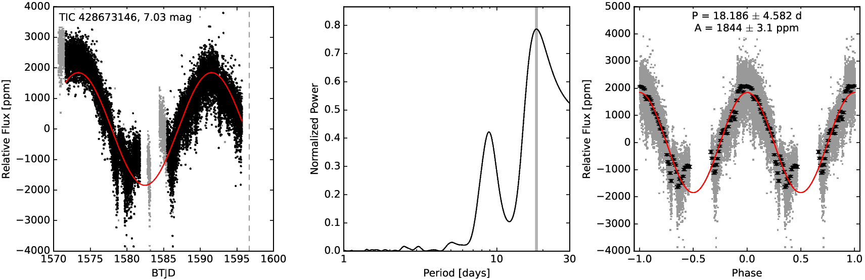
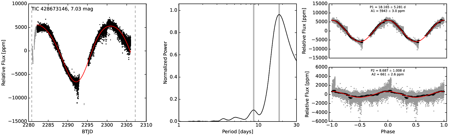
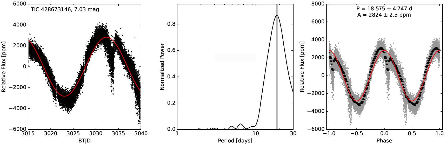
Figure 1: TESS 2-minute cadence photometry (left column), Lomb-Scargle periodogram (center column), and light curve phase-folded on the measured stellar rotation period (right column) for sectors 10 (top row), 36 (center row), and 63 (bottom row). The gray points in the left column panels show data points that were removed based on poor quality flags or 5$\sigma$ outliers. The red curve represents the sinusoidal function that best-fits the light curve and represents the measured stellar rotation period. The black points in the right column represent the binned photometry.

As mentioned in Section 2.2, we used a Lomb-Scargle periodogram to examine stellar variability that may be associated with the rotation period of the star from each individual sector of TESS photometry. Shown in Figure 1 are the photometry, periodogram analysis, and folded lightcurves for TESS sectors 10 (top row), 36 (middle row), and 63 (bottom row). These analyses reveal a consistent periodic variability signature of $18.3\pm 4.9$ days for the three sectors, despite the observations each being separated by $\sim$1 year. The second period identified in sector 36 is approximately half of the primary variability period, and thus is likely an alias. If the 18.3 day signal is indeed the signature of the stellar rotation period, then it is quite different from that derived spectroscopically by Ségransan et al. (2011) and Suárez Mascareño et al. (2015). A possible cause of this discrepancy in rotation period measurements is differential rotation, similar to that observed for the known exoplanet host HD 219134 (Johnson et al., 2016). Furthermore, there is growing evidence that spectroscopic and photometric rotation period measurements do not always agree, possibly the result of activity differences in the chromosphere and photosphere (Lafarga et al., 2021; Schöfer et al., 2022; Isaacson et al., 2024). However, there are several other pieces of information to note here. First, the $R_{\star}$ and $v\sin i$ values shown in Table 1 result in a calculated rotation period of $\sim$17 days, which is more consistent with the rotation period derived from TESS photometry than those previously determined spectroscopically. Ségransan et al. (2011) measured a $v\sin i=1.61$ km/s; slower than the 2.32 km/s value shown in Table 1, and enough to account for their larger rotation period of $\sim$30 days. Second, the TESS photometry is substantially separated in time from the HARPS RV data, such that the star may be located at a significantly different place within its magnetic activity cycle, as has been photometrically observed for numerous other stars (Henry et al., 2000; Dragomir et al., 2012). Third, it is worth acknowledging that aliases of the true rotation period can be difficult to disentangle, depending on the sampling rate of the observations, and so some of the reported rotation periods may be examples of such aliases.

3.2 Non-Transiting Planets

3.2.1 Radial Velocity Solutions

We utilized both HARPS and HIRES data in our RV analysis. In our modeling process, we divided the HIRES dataset into two separate datasets (HIRES1 and HIRES2) due to a major upgrade carried out on HIRES in August 2004 (Butler et al., 2017) that could introduce a velocity offset between the two datasets. We first used an iterative planet search tool, RVSearch, to look for potential planetary signals within the combined data. We refer readers to Rosenthal et al. (2021) for details regarding the working process of RVSearch. We set the algorithm to search within a period space between 2 days and five times the combined observing baseline of HARPS and HIRES, which is around 48,000 days. The search process includes instrument offsets as well as linear and quadratic trends, and we only considered periodogram signals that have a false alarm probability (FAP) less than 0.1%, as described by Howard & Fulton (2016) and Fulton et al. (2018). RVSearch returned two significant signals from the search: one belonging to the known b planet at $\sim$58 days with an FAP that is consistent with zero, and the other yielding a new period signature of $\sim$14 days with an FAP of $3.29\times 10^{-7}$. It is worth noting that the 14 day signal is primarily detectable within the HARPS data, which is unsurprising given the high cadence nature of the HARPS observations as well as their slightly higher RV precision compared to the HIRES data.

The RVSearch results were then used as input for the RV modeling toolkit RadVel (Fulton et al., 2018) to sample posteriors of Keplerian orbital parameters of the returned signals, as well as to estimate the associated uncertainties via a Markov Chain Monte Carlo (MCMC) analysis. All parameters, including instrument offset and trends, were allowed to vary as free parameters. Chain convergences were evaluated under four criteria: Gelman-Rubin statistic ($<0.01$), minimum autocorrelation time factor ($>40$), maximum relative change in autocorrelation time ($<0.03$), and minimum independent draws ($>1000$). The MCMC chain rapidly converged, and we present the full results of our two planet model in Table 2. The planetary masses and semi-major axes were derived using the stellar mass shown in Table 1. The model includes both a linear and a quadratic trend, with significances of 3$\sigma$ and 2$\sigma$, respectively. The RV data are shown in Figure 2, where the blue lines indicate the best fit to the data. The top panels show the full observational baseline and the residuals from the fit to the data. The bottom panels show the individual fits to the two planetary signatures detected in the RV data: the known 55.8 day period planet (planet b), and the newly detected 13.9 day period planet (planet c).

Table 2: Radial velocity derived planetary parameters.

Parameter	Credible Interval	Maximum Likelihood	Units
Orbital Parameters
$P_{b}$	$55.851\pm 0.017$	$55.851$	days
$T\rm{conj}_{b}$	$2454167.3^{+0.94}_{-0.87}$	$2454167.0$	BJD
$T\rm{peri}_{b}$	$2454159.5^{+3.5}_{-3.4}$	$2454159.7$	BJD
$e_{b}$	$0.123^{+0.048}_{-0.051}$	$0.136$
$\omega_{b}$	$0.5^{+0.4}_{-0.41}$	$0.5$	radians
$K_{b}$	$12.0\pm 0.57$	$11.98$	m s-1
$P_{c}$	$13.8992^{+0.0047}_{-0.0037}$	$13.8985$	days
$T\rm{conj}_{c}$	$2455192.9^{+0.59}_{-0.56}$	$2455192.64$	BJD
$T\rm{peri}_{c}$	$2455191.6^{+1.2}_{-1.1}$	$2455191.6$	BJD
$e_{c}$	$0.29^{+0.12}_{-0.13}$	$0.32$
$\omega_{c}$	$0.64^{+0.57}_{-0.56}$	$0.66$	radians
$K_{c}$	$4.25^{+0.62}_{-0.63}$	$4.49$	m s-1
Other Parameters
$\gamma_{\rm HIRES2}$	$-1.81^{+0.72}_{-0.74}$	$-1.59$	m s$-1$
$\gamma_{\rm HIRES1}$	$0.0^{+2.6}_{-2.8}$	$0.4$	m s$-1$
$\gamma_{\rm HARPS}$	$1.02^{+0.84}_{-0.82}$	$1.14$	m s$-1$
$\dot{\gamma}$	$0.0013^{+0.00042}_{-0.00043}$	$0.00142$	m s-1 d-1
$\ddot{\gamma}$	$2.7e-07\pm 1.3e-07$	$2.7e-07$	m s-1 d-2
$\sigma_{\rm HIRES2}$	$4.34^{+0.6}_{-0.52}$	$3.85$	$\rm m\ s^{-1}$
$\sigma_{\rm HIRES1}$	$8.2^{+1.1}_{-1.2}$	$8.1$	$\rm m\ s^{-1}$
$\sigma_{\rm HARPS}$	$4.05^{+0.37}_{-0.33}$	$3.83$	$\rm m\ s^{-1}$
Derived Posteriors
$M_{b}\sin i$	$62.1^{+3.3}_{-3.2}$	$61.5$	M⊕
$a_{b}$	$0.2674^{+0.0032}_{-0.0033}$	$0.2671$	AU
$M_{c}\sin i$	$13.2\pm 1.9$	$13.2$	M⊕
$a_{c}$	$0.1058\pm 0.0013$	$0.1057$	AU

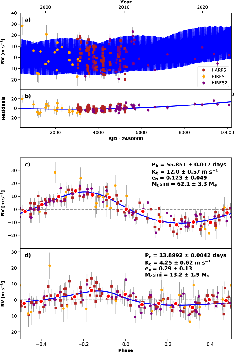
Figure 2: RV data for HD 104067, including those acquired from HARPS and HIRES on either side of the 2004 HIRES upgrade (HIRES1 and HIRES2), where the blue lines indicate the best fit to the data. The top panels show the full observational baseline and fit to the residuals. The bottom panels show the data fits for the individual planets, b and c.

3.2.2 Planet Search Completeness

We carried out an injection and recovery test on the combined HARPS and HIRES RV data to examine the sensitivity of RV data to potential additional companions in the system. In total, 3000 synthetic planets were injected into the data, with orbital eccentricities drawn from a beta distribution using parameters from Kipping (2013), and orbital periods and minimum masses drawn from log-uniform distributions. We then used the results from the injection and recovery test to compute a search completeness contour, shown in Figure 3 as a function of mass ($M_{p}\sin i$) and semi-major axis ($a$). The two recovered signals described in Section 3.2.1 are marked as solid black dots with the $\sim$14-day signal lying on the 50% completeness curve, indicated by the black line. The individual blue and red dots indicate whether the recovery was successful at each injected location. The results suggest that additional giant planets more massive than the already discovered planet b are clearly recoverable if present in the inner part of the system, but were not detected within our data, suggesting that such an additional planetary presence is extremely unlikely within 1–2 AU of the host star. However, our data do not rule out their presence beyond 10 AU, which corresponds roughly to the observing baseline of the combined RV dataset. On the other hand, smaller planets less massive than 10 Earth masses lie below the 50% completeness curve for the majority of the parameter space, hinting the possibility that small planets may yet be present within the system. These small planets sit below the sensitivity of our RV data and their discoveries require further observations and/or more precise measurements. Overall, our injection-recovery analysis is able to exclude Saturn-mass and Jupiter-mass planets out to 3 AU and 8 AU, respectively. It is worth noting that the completeness analysis described here refers to $M_{p}\sin i$, and so depends on the inclination of the synthetic planetary orbits relative to the plane of the sky.

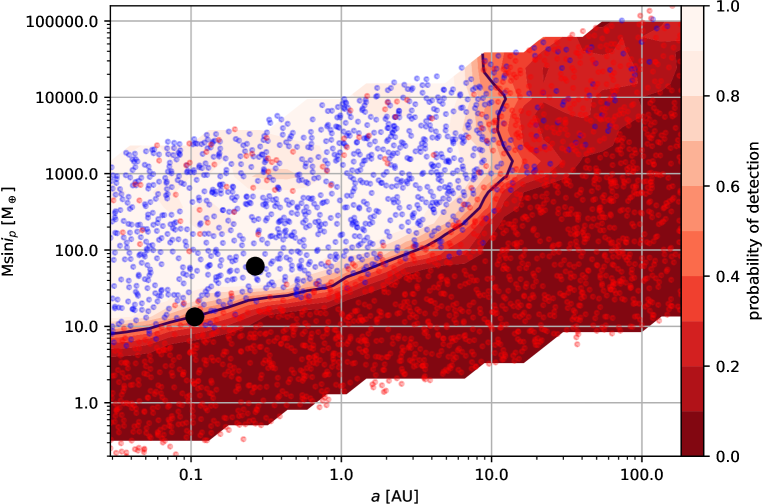
Figure 3: Results of the injection-recovery test to determine the sensitivity of the RV data to planetary signatures as a function of planetary mass ($M_{p}\sin i$) and semi-major axis ($a$). The blue dots represent injected planetary signatures that were successfully recovered and the red dots represent those planets that were not recovered. The color scale shown on the right vertical axis corresponds to the probability contours of detecting a planet of a given mass and semi-major axis. The two detected planets are shown as large black dots.

3.2.3 Stellar Activity

Periodic stellar activity cycles, such as rotation, long term magnetic cycles, and their aliases, can mimic RV signatures similar to those induced by exoplanets and therefore sometimes could be mistakenly identified as exoplanet candidates (Desort et al., 2007; Robertson et al., 2014; Kane et al., 2016). As a crucial step in all exoplanet discovery and follow-up work, it is essential to check whether activity could be the primary source contributing to the periodicities identified in the RV time series. Here, we make use of all available stellar activity indicators for both HARPS and HIRES to check if any of the activity periods coincide with our identified RV signals in Section 3.2.1. For HARPS, we used all available activity indicators provided within the HARPS RV database (Trifonov et al., 2020), namely the H$\alpha$ index, chromatic index, differential line width, Na I D index, Na II D index, cross correlation function (CCF) bisector inverse slope span, CCF full width at half maximum, and CCF contrast. In addition, we include Ca II H & K measurements from the second version of the HARPS RV database (Perdelwitz et al., 2023). For HIRES, the Ca II H & K time series serve as the only activity indicator. All activity time series were passed through a Generalized Lomb-Scargle periodogram (Zechmeister & Kürster, 2009) to check for periodic signals within the observing baseline. No peak in the activity periodograms were found to be located on or near the periodicities of the two recovered RV signals described in Section 3.2.1. These results suggest that the planetary nature of the newly recovered $\sim$14-day signal is likely genuine.

3.3 An Inner Transiting Planet Candidate

As described in Section 2.2, the TESS photometry consists of three sectors: 10, 36, and 63. For the analysis of the transit signal, designated as TOI-6713.01, we used the LightKurve package (Lightkurve Collaboration et al., 2018) to download the relevant sectors of the PDC and SAP time series measurements from MAST. We prepared the data by first using a Savitzky–Golay filter (Savitzky & Golay, 1964) to temporarily flatten the light curve after masking out the transits (with one transit duration on either side). An outlier mask was created by performing 5 iterations of 3$\sigma$ clipping on the flattened light curve. We then also removed segments of the light curve that were heavily affected by momentum dumps. This, in addition to the outlier mask, removed $\sim$8% of the light curve data.

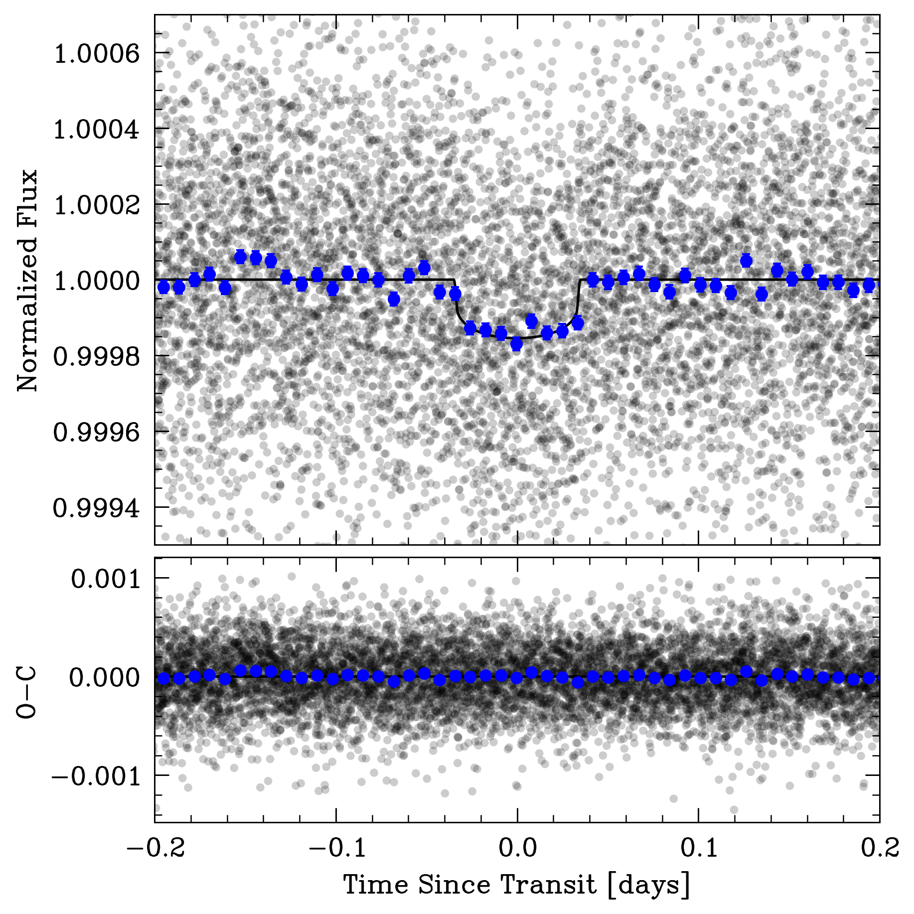
Figure 4: Folded TESS light curve, where gray points are the raw data and blue represent the binned data. The median transit model is plotted as the black line. Residuals (data minus model) are shown in the lower panel.

Table 3: TOI-6713.01 TESS Transit Parameters

Parameter [units]	Credible Interval	Source
Transit Parameters
$P$ [days]	$2.1538197\pm 0.0000041$	This work, fit
$T\rm{conj}$ [BJD${}_{\text{TDB}}-2457000.0$]	$1571.52211\pm 0.00081$	This work, fit
$R_{p}/R_{\star}$ [–]	$0.0152\pm 0.0014$	This work, fit
$T_{14}$ [hours]	$1.667\pm 0.065$	This work, fit
$b$ [–]	$0.52\pm 0.29$	This work, fit
$e$ [–]	$\equiv 0$	This work
$\omega$ [–]	$\equiv 0$	This work
$R_{p}$ [$R_{\oplus}$]	$1.30\pm 0.12$	This work, derived
$a/R_{\star}$ [–]	$8.42\pm 0.15$	This work, derived
$a$ [AU]	$0.03054\pm 0.00037$	This work, derived
$i$ [deg]	$86.5\pm 2.0$	This work, derived
Gaussian Process Parameters
$\ln{(Q)}$ [–]	$-6.59\pm 0.53$	This work, fit
$\ln{(dQ)}$ [–]	$-1.43\pm 0.75$	This work, fit
$P_{\text{rot}}$ [days]	$8.9\pm 2.6$	This work, fit
$\ln{(\sigma)}$ [–]	$-8.30\pm 0.12$	This work, fit
$f$ [–]	$0.093\pm 0.025$	This work, fit

We fit the prepared light curve using the exoplanet package (Foreman-Mackey et al., 2021), which uses a Hamiltonian Monte Carlo (HMC) routine to explore posterior probability distributions. To model the transit, we assumed a circular orbit with orbital period ($P$), time of inferior conjunction ($T_{\mathrm{conj}}$), scaled planet radius ($R_{p}/R_{\star}$), impact parameter ($b$), transit duration ($T_{14}$), and mean flux offset ($\mu$) as free parameters. Quadratic limb darkening coefficients were held constant at $u_{0}=0.45$ and $u_{1}=0.18$ (Claret, 2017). Gaussian priors were set on $P$ and $T_{\mathrm{conj}}$ based on values reported by the Exoplanet Follow-up Observing Program (ExoFOP).

The stellar variability was modeled using the RotationTerm kernel included in celerite2 (Foreman-Mackey et al., 2017), which is a mixture of two simple harmonic oscillators. For the secondary oscillation quality factor ($Q$), the difference in quality factors between the primary and secondary modes ($dQ$), fractional amplitude of secondary mode relative to primary mode ($f$), and the standard deviation of the GP ($\sigma$), we sampled the logarithmic value of the parameter. A Gaussian prior was placed on the rotation period ($P_{\text{rot}}$) informed by the stellar activity analysis in Section 3.1. However we note the 18 day signal was not well-preserved in the PDC lightcurve.

We used the values obtained from minimizing a negative log-likelihood function as initial positions for two parallel chains and ran the HMC for 2000 tuning steps and 4000 sampling steps per chain. In Table 3 we provide the median values with their 1$\sigma$ uncertainties for each fitted and derived parameter. The model fit to binned TESS data is shown in Figure 4. The transit depth is 231 ppm and the out-of-transit PDCSAP photometry has a standard deviation of $\sim$300 ppm. As there are $\sim$1300 measurements acquired during transit, the transit signal-to-noise for this detection is $S/N\sim 27$, according to the methodology described by Pont et al. (2006). Note that we examined both the PDC and SAP photometry from the individual TESS sectors and found that the transit signal was present in all cases, although the signal becomes less significant in the SAP data. More follow-up observations are needed to validate and confirm the planetary nature of the photometric signal.

4 Orbital Dynamics

Here we present results of a dynamical analysis of the system, including tidal impacts for the inner transiting planet candidate.

4.1 Long-Term Stability

Given the eccentric orbits of the RV-detected giant planets, and the prospect of a further inner terrestrial planet (see Section 3), the architecture of the system presents an interesting opportunity to explore planetary dynamical interactions within a relatively compact system. The dynamical simulations conducted for this work make use of the Mercury Integrator Package (Chambers, 1999), using similar methodology to that conducted by Kane (2019); Kane et al. (2021a). We also adopt the hybrid symplectic/Bulirsch-Stoer integrator with a Jacobi coordinate system, which generally provides more accurate results for multi-planet systems (Wisdom & Holman, 1991; Wisdom, 2006). We used a time step of 0.05 days (1.2 hours) to ensure adequate sampling of the inner planetary orbit and ran the simulation for a $10^{7}$ years. Although neither of the two RV planets are known to transit, we assumed that the system is roughly coplanar. Adopting the parameters for the inner planet described in Section 3.3, we assumed a circular orbit for that planet. Given the estimated radius for the inner planet of $1.30\pm 0.12$ $R_{\oplus}$, we adopted a planetary mass of 2 $M_{\oplus}$, based on predictions from exoplanet mass-radius relationships (Weiss & Marcy, 2014; Chen & Kipping, 2017).

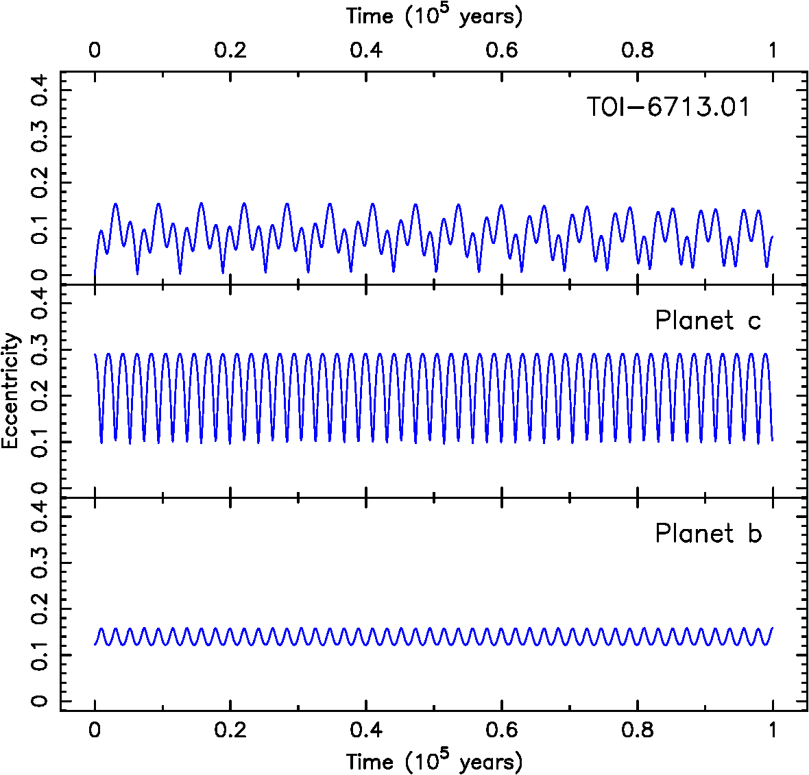
Figure 5: Eccentricity evolution for the three planet model of the HD 104067 system, including the transiting planet candidate, TOI-6713.01 (top panel), the newly detected planet c (middle panel), and the previously known planet b (bottom panel). Data are shown for the first $10^{5}$ years of the full $10^{7}$ year integration.

Our simulations found that the system is able to retain long-term stability for the full $10^{7}$ year integration. The results of our simulations are represented in Figure 5, showing the eccentricity evolution of the transiting planet candidate, TOI-6713.01 (top panel), the newly detected planet c (middle panel), and the previously known planet b (bottom panel). In order for the structure of the eccentricity evolution to be easily visible, we have restricted the data shown in the plot to the first $10^{5}$ years of the full $10^{7}$ year simulation. Note also that we use identical eccentricity scales for each panel to emphasize the relative amplitudes of the eccentricity variations. Figure 5 shows that the two giant planets experience a regular exchange of angular momentum that results in eccentricity ranges of 0.12–0.16 and 0.10–0.29 for planets b and c, respectively. The eccentricity range for TOI-6713.01 is 0.00–0.16, with a clear beating pattern, indicating that the presence of the inner planet causes a slight difference in frequency between the angular moment exchange between planets b and c. Since TOI-6713.01 lies so close to the host star, even a relatively small eccentricity excitation may have significant consequences for tidal forces experienced by the planet.

4.2 Tidal Effects

Based on the eccentricity evolution resulting from the dynamical simulations from Section 4.1, we calculated the tidal heating of the inner planet candidate and the consequences for the planetary surface temperature. The power contributed to a rigid body via tidal heating is given by

$$P_{\mathrm{tides}}=\dot{E}=-\mathrm{Im}(k_{2})\frac{21}{2}\frac{G^{3/2}M_{\star}^{5/2}R_{p}^{5}e^{2}}{a^{15/2}}$$ (1)

where $G$ is the gravitational constant, $M_{\star}$ is the mass of the host star, $R_{p}$ is the radius of the planet, $e$ is the orbital eccentricity, and $k_{2}$ is the second-order Love number (Squyres et al., 1983; Meyer & Wisdom, 2007). For our calculations, we adopt a Love number of $k_{2}=0.35$, based on the terrestrial bodies (Zhang, 1992). Equation 1 clearly demonstrates the extreme sensitivity of tidal heating and power output to the semi-major axis of the body, since it scales with $a^{-15/2}$. For example, the tidal heating of Io results in a total tidal dissipation of $10^{14}$ W (Bierson & Steinbrügge, 2021).

The proximity of TOI-6713.01 to the host star will also result in significant incident flux of stellar radiation that contributes to the overall energy budget of the planet. The power absorbed by the planet due to the star is given by

$$P_{\mathrm{star}}=\frac{L_{\star}}{4\pi a^{2}}(1-A)\pi R_{p}^{2}$$ (2)

where $L_{\star}$ is the stellar luminosity and $A$ is the Bond albedo of the planet. In order to set an upper limit on the stellar contribution to the planetary heating, we adopt a Bond albedo of $A=0.0$. For epochs of the simulated dynamical evolution where the planet has a non-zero eccentricity, we consider only the average flux received and so evaluate Equation 2 at the semi-major axis.

To calculate the total power emitted by the planet, we consider the planet using a blackbody approximation such that the power radiated by the planet may be expressed as

$$P_{\mathrm{rad}}=4\pi R_{p}^{2}\epsilon\sigma T_{p}^{4}$$ (3)

where $\epsilon$ is the emissivity of the planet, $\sigma$ is the Stefan–Boltzmann constant, and $T_{p}$ is the blackbody equilibrium temperature of the planet. We assume an emissivity of $\epsilon=1.0$ which treats the planet as a perfect emitter. As a blackbody, the power radiated equates to the total power absorbed ($P_{\mathrm{star}}+P_{\mathrm{tides}}$). The equilibrium temperature of the planet is therefore provided by

$$T_{p}=\left(\frac{P_{\mathrm{star}}+P_{\mathrm{tides}}}{4\pi R_{p}^{2}\epsilon\sigma}\right)^{\frac{1}{4}}$$ (4)

where the power calculations of Equation 1 and Equation 2 have been incorporated.

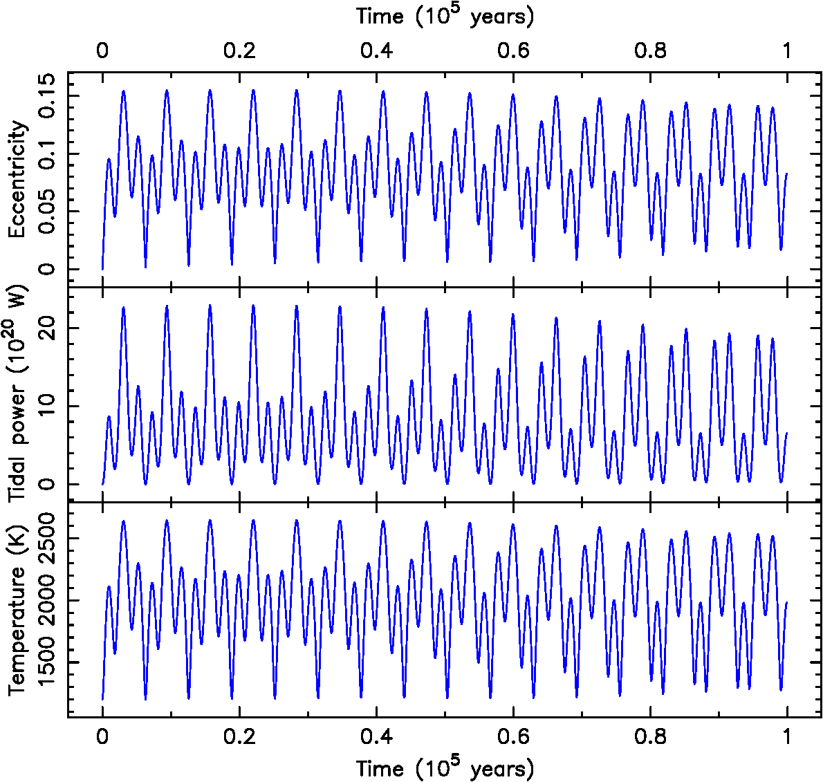
Figure 6: The eccentricity (top panel), tidal power (middle panel), and equilbrium temperature (bottom panel) evolution of the transiting planet candidate, TOI-6713.01. As for Figure 5, these results are shown for the first $10^{5}$ years of the dynamical simulation.

Figure 6 shows the results of our tidal effects calculations for TOI-6713.01 for the first $10^{5}$ years of the eccentricity evolution (see Section 4.1). The top panel shows an expanded view of the eccentricity evolution of the planet candidate. The middle panel shows the tidal energy dissipation rate (power) emitted by the planet (Equation 1). The bottom panel shows the equilibrium temperature of the planet, combining the effects of tidal energy and incident stellar flux (Equation 4). Clearly, the proximity of the planet to the host star results in a highly sensitive response of the planet’s tidal energy to the eccentricity variations. The mean tidal power produced by the planet is $8.3\times 10^{20}$ W, or almost 7 orders of magnitude larger than Io. Amazingly, using the above mentioned assumptions regarding Love number, Bond albedo, and emissivity, these calculations lead to a very high equilibrium temperature for the planet, where the temperature varies in the range 1202–2646 K. For an emissivity of $\epsilon=0.5$, the equilibrium temperature raises even higher, reaching peak values of 3130 K. In either scenario, the peak value of the temperature evolution is well above that needed for the surface to be in an entirely molten state (Boukaré et al., 2022).

5 Discussion

Like many systems that are subjected to detailed follow-up observations, the HD 104067 system has revealed itself to be increasingly complex. The additional RV-detected planet (planet c) provides a potential source for the eccentricity of the previously known giant planet. The potential for the existence of an inner terrestrial planet creates a fascinating architecture that is almost optimal for maximizing the tidal power emission of the planet. However, TOI-6713.01 has yet to be confirmed. Though the transiting planet candidate was detected in a known exoplanet system and the period of the transits is significantly different from the estimates of intrinsic stellar variability, there remains the possibility that the transit signal is caused by a false-alarm scenario. The relatively large pixel sizes of TESS can result in substantial blending from background stars, creating diluted signals via blended eclipsing binary stars that can mimic transit signatures (Brown, 2003; Pont et al., 2006; Bryson et al., 2013; Fressin et al., 2013) or effect the derived planetary radius (Ciardi et al., 2015). A typical pathway to remedy the risk of false-alarm signals is RV follow-up that is able to successfully extract a planetary mass (Chontos et al., 2022), and/or the use of validation steps that search for blend contamination (Giacalone et al., 2021), including high resolution imaging that may detect nearby stellar companions within the photometric aperture (Howell et al., 2011; Matson et al., 2019; Schlieder et al., 2021). Although substantial efforts toward the imaging of bright exoplanet host stars has been carried out (Kane et al., 2014, 2015; Wittrock et al., 2016, 2017), much of such efforts have been directed toward hosts of transiting planets for validation purposes (Law et al., 2014; Howell et al., 2021). Furthermore, assuming a planet mass of 2 $M_{\oplus}$, TOI-6713.01 would have an expected RV amplitude of $\sim$1 m/s, comparable to the RV precision of both HARPS and HIRES (see Section 2.1) and significantly below the completeness contour shown in Figure 3. The RV completeness results also rule out minimum masses for the transiting planet candidate greater than $\sim$10 $M_{\oplus}$, excluding scenarios such as a grazing stellar companion. Given the brightness of the host star and the history of previous observations, it is unlikely that stellar blends are the cause of the transit signature detected by TESS. However, further observations are recommended to validate the planetary nature of the transit signal.

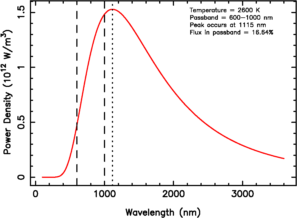
Figure 7: The predicted blackbody flux of TOI-6713.01, assuming a calculated temperature of $\sim$2600 K. The passband boundaries of TESS are indicated by the vertical dashed lines. Of the integrated flux, 16.64% falls within the TESS passband.

If the transiting planet candidate can be validated, then it may present an interesting target to determine upper limits on the effects of tidal heating, described in Section 4.2. An important factor in ascertaining the viability of such follow-up observations is the calculation of predicted flux emission in the context of expected observational bandpasses. For example, shown in Figure 7 is the predicted blackbody spectrum (red line), assuming the peak equilibrium temperature of 2600 K, as estimated in Section 4.2. The vertical lines indicate the passband boundaries of the TESS instrumentation (600nm–1000nm). Of the integrated flux from the thermal emission, $\sim$16.64% of the total flux falls within the passband of the TESS observations. In terms of wavelength-dependent flux ratios with the host star, the expected flux ratios are 83, 92, and 107 ppm at 3.6, 4.5, and 8.0 microns, respectively. The cause of the relatively small amplitude of these signatures, despite the high equilibrium temperature, is dominated by the relatively small size of the planet. Note that, as described in Section 4.2, the amplitude of these signatures will vary with time, and often be significantly lower than these peak values. Moreover, the amplitude of these signatures are below the measured transit depth (see Section 3.3) and so will be challenging to detect within TESS photometry.

6 Conclusions

The incredible diversity of observed planetary architectures have also led to a plethora of dynamical scenarios that deviate substantially from those observed in the solar system. The opportunities to perform detailed follow-up studies are often best afforded by systems for which RV exoplanet detections have been made, since these preferentially have bright host stars compared with those systems detected through the transit method. Thus, when transits are detected in known RV systems, there are often interesting opportunities to characterize planetary orbits and atmospheres where there has already been a long history of observations. The HD 104067 system is proving to be such a case. Our detection of a further giant planet in an eccentric orbit reveals a compact architecture with a complex dynamical environment. The potential addition of a short period terrestrial planet results in an injection of tidal energy into the planet that has rarely been seen before, and a case study of possible magma oceans that may have a detectable signature. Our calculations for the equilibrium temperature of the inner planet candidate lie in the range 1202–-2646 K, including the effects of extreme stellar flux and cyclic tidal energy resulting from the eccentricity evolution. Though the RV and thermal signatures of the inner planet lie at the threshold of current instruments and facilities, the continual improvement of measurements for this system may enable observational tests of the calculations presented here, providing insight into the formation and evolution of compact planetary systems.

References

- Bierson & Steinbrügge (2021) Bierson, C. J., & Steinbrügge, G. 2021, \psj, 2, 89, doi: 10.3847/PSJ/abf48d
- Bonomo et al. (2023) Bonomo, A. S., Dumusque, X., Massa, A., et al. 2023, A&A, 677, A33, doi: 10.1051/0004-6361/202346211
- Borucki (2016) Borucki, W. J. 2016, Reports on Progress in Physics, 79, 036901, doi: 10.1088/0034-4885/79/3/036901
- Boukaré et al. (2022) Boukaré, C.-É., Cowan, N. B., & Badro, J. 2022, ApJ, 936, 148, doi: 10.3847/1538-4357/ac8792
- Brown (2003) Brown, T. M. 2003, ApJ, 593, L125, doi: 10.1086/378310
- Bryson et al. (2013) Bryson, S. T., Jenkins, J. M., Gilliland, R. L., et al. 2013, PASP, 125, 889, doi: 10.1086/671767
- Butler et al. (2017) Butler, R. P., Vogt, S. S., Laughlin, G., et al. 2017, AJ, 153, 208, doi: 10.3847/1538-3881/aa66ca
- Chambers (1999) Chambers, J. E. 1999, MNRAS, 304, 793, doi: 10.1046/j.1365-8711.1999.02379.x
- Chen & Kipping (2017) Chen, J., & Kipping, D. 2017, ApJ, 834, 17, doi: 10.3847/1538-4357/834/1/17
- Chontos et al. (2022) Chontos, A., Murphy, J. M. A., MacDougall, M. G., et al. 2022, AJ, 163, 297, doi: 10.3847/1538-3881/ac6266
- Ciardi et al. (2015) Ciardi, D. R., Beichman, C. A., Horch, E. P., & Howell, S. B. 2015, ApJ, 805, 16, doi: 10.1088/0004-637X/805/1/16
- Claret (2017) Claret, A. 2017, A&A, 600, A30, doi: 10.1051/0004-6361/201629705
- Desort et al. (2007) Desort, M., Lagrange, A. M., Galland, F., Udry, S., & Mayor, M. 2007, A&A, 473, 983, doi: 10.1051/0004-6361:20078144
- Dragomir et al. (2012) Dragomir, D., Kane, S. R., Henry, G. W., et al. 2012, ApJ, 754, 37, doi: 10.1088/0004-637X/754/1/37
- Dragomir et al. (2020) Dragomir, D., Harris, M., Pepper, J., et al. 2020, AJ, 159, 219, doi: 10.3847/1538-3881/ab845d
- Fischer et al. (2016) Fischer, D. A., Anglada-Escude, G., Arriagada, P., et al. 2016, PASP, 128, 066001, doi: 10.1088/1538-3873/128/964/066001
- Ford (2014) Ford, E. B. 2014, Proceedings of the National Academy of Science, 111, 12616, doi: 10.1073/pnas.1304219111
- Foreman-Mackey et al. (2017) Foreman-Mackey, D., Agol, E., Ambikasaran, S., & Angus, R. 2017, AJ, 154, 220, doi: 10.3847/1538-3881/aa9332
- Foreman-Mackey et al. (2021) Foreman-Mackey, D., Luger, R., Agol, E., et al. 2021, The Journal of Open Source Software, 6, 3285, doi: 10.21105/joss.03285
- Fressin et al. (2013) Fressin, F., Torres, G., Charbonneau, D., et al. 2013, ApJ, 766, 81, doi: 10.1088/0004-637X/766/2/81
- Fulton et al. (2018) Fulton, B. J., Petigura, E. A., Blunt, S., & Sinukoff, E. 2018, PASP, 130, 044504, doi: 10.1088/1538-3873/aaaaa8
- Fulton et al. (2021) Fulton, B. J., Rosenthal, L. J., Hirsch, L. A., et al. 2021, ApJS, 255, 14, doi: 10.3847/1538-4365/abfcc1
- Gaia Collaboration et al. (2021) Gaia Collaboration, Brown, A. G. A., Vallenari, A., et al. 2021, A&A, 649, A1, doi: 10.1051/0004-6361/202039657
- Giacalone et al. (2021) Giacalone, S., Dressing, C. D., Jensen, E. L. N., et al. 2021, AJ, 161, 24, doi: 10.3847/1538-3881/abc6af
- Guerrero et al. (2021) Guerrero, N. M., Seager, S., Huang, C. X., et al. 2021, ApJS, 254, 39, doi: 10.3847/1538-4365/abefe1
- He et al. (2019) He, M. Y., Ford, E. B., & Ragozzine, D. 2019, MNRAS, 490, 4575, doi: 10.1093/mnras/stz2869
- Henry et al. (2000) Henry, G. W., Fekel, F. C., Henry, S. M., & Hall, D. S. 2000, ApJS, 130, 201, doi: 10.1086/317346
- Horner et al. (2020) Horner, J., Kane, S. R., Marshall, J. P., et al. 2020, PASP, 132, 102001, doi: 10.1088/1538-3873/ab8eb9
- Howard & Fulton (2016) Howard, A. W., & Fulton, B. J. 2016, PASP, 128, 114401, doi: 10.1088/1538-3873/128/969/114401
- Howell et al. (2011) Howell, S. B., Everett, M. E., Sherry, W., Horch, E., & Ciardi, D. R. 2011, AJ, 142, 19, doi: 10.1088/0004-6256/142/1/19
- Howell et al. (2021) Howell, S. B., Matson, R. A., Ciardi, D. R., et al. 2021, AJ, 161, 164, doi: 10.3847/1538-3881/abdec6
- Huang et al. (2018) Huang, C. X., Burt, J., Vanderburg, A., et al. 2018, ApJ, 868, L39, doi: 10.3847/2041-8213/aaef91
- Huber et al. (2017) Huber, D., Zinn, J., Bojsen-Hansen, M., et al. 2017, ApJ, 844, 102, doi: 10.3847/1538-4357/aa75ca
- Ida et al. (2013) Ida, S., Lin, D. N. C., & Nagasawa, M. 2013, ApJ, 775, 42, doi: 10.1088/0004-637X/775/1/42
- Isaacson et al. (2024) Isaacson, H., Kane, S. R., Carter, B., et al. 2024, ApJ, 961, 85, doi: 10.3847/1538-4357/ad077b
- Jenkins et al. (2016) Jenkins, J. M., Twicken, J. D., McCauliff, S., et al. 2016, in Proc. SPIE, Vol. 9913, Software and Cyberinfrastructure for Astronomy IV, 99133E, doi: 10.1117/12.2233418
- Johnson et al. (2016) Johnson, M. C., Endl, M., Cochran, W. D., et al. 2016, ApJ, 821, 74, doi: 10.3847/0004-637X/821/2/74
- Jurić & Tremaine (2008) Jurić, M., & Tremaine, S. 2008, ApJ, 686, 603, doi: 10.1086/590047
- Kane (2019) Kane, S. R. 2019, AJ, 158, 72, doi: 10.3847/1538-3881/ab2a09
- Kane et al. (2021a) Kane, S. R., Li, Z., Wolf, E. T., Ostberg, C., & Hill, M. L. 2021a, AJ, 161, 31, doi: 10.3847/1538-3881/abcbfd
- Kane et al. (2009) Kane, S. R., Mahadevan, S., von Braun, K., Laughlin, G., & Ciardi, D. R. 2009, PASP, 121, 1386, doi: 10.1086/648564
- Kane & Raymond (2014) Kane, S. R., & Raymond, S. N. 2014, ApJ, 784, 104, doi: 10.1088/0004-637X/784/2/104
- Kane et al. (2014) Kane, S. R., Howell, S. B., Horch, E. P., et al. 2014, ApJ, 785, 93, doi: 10.1088/0004-637X/785/2/93
- Kane et al. (2015) Kane, S. R., Barclay, T., Hartmann, M., et al. 2015, ApJ, 815, 32, doi: 10.1088/0004-637X/815/1/32
- Kane et al. (2016) Kane, S. R., Thirumalachari, B., Henry, G. W., et al. 2016, ApJ, 820, L5, doi: 10.3847/2041-8205/820/1/L5
- Kane et al. (2020) Kane, S. R., Yalçınkaya, S., Osborn, H. P., et al. 2020, AJ, 160, 129, doi: 10.3847/1538-3881/aba835
- Kane et al. (2021b) Kane, S. R., Arney, G. N., Byrne, P. K., et al. 2021b, Journal of Geophysical Research (Planets), 126, e06643, doi: 10.1002/jgre.v126.2
- Kane et al. (2021c) Kane, S. R., Bean, J. L., Campante, T. L., et al. 2021c, PASP, 133, 014402, doi: 10.1088/1538-3873/abc610
- Kipping (2013) Kipping, D. M. 2013, MNRAS, 434, L51, doi: 10.1093/mnrasl/slt075
- Lafarga et al. (2021) Lafarga, M., Ribas, I., Reiners, A., et al. 2021, A&A, 652, A28, doi: 10.1051/0004-6361/202140605
- Law et al. (2014) Law, N. M., Morton, T., Baranec, C., et al. 2014, ApJ, 791, 35, doi: 10.1088/0004-637X/791/1/35
- Lightkurve Collaboration et al. (2018) Lightkurve Collaboration, Cardoso, J. V. d. M. a., Hedges, C., et al. 2018, Lightkurve: Kepler and TESS time series analysis in Python, . http://ascl.net/1812.013
- Martin & Livio (2015) Martin, R. G., & Livio, M. 2015, ApJ, 810, 105, doi: 10.1088/0004-637X/810/2/105
- Matson et al. (2019) Matson, R. A., Howell, S. B., & Ciardi, D. R. 2019, AJ, 157, 211, doi: 10.3847/1538-3881/ab1755
- Meyer & Wisdom (2007) Meyer, J., & Wisdom, J. 2007, Icarus, 188, 535, doi: 10.1016/j.icarus.2007.03.001
- Mishra et al. (2023) Mishra, L., Alibert, Y., Udry, S., & Mordasini, C. 2023, A&A, 670, A68, doi: 10.1051/0004-6361/202243751
- Pepe et al. (2000) Pepe, F., Mayor, M., Delabre, B., et al. 2000, in Society of Photo-Optical Instrumentation Engineers (SPIE) Conference Series, Vol. 4008, Proc. SPIE, ed. M. Iye & A. F. Moorwood, 582–592, doi: 10.1117/12.395516
- Pepper et al. (2020) Pepper, J., Kane, S. R., Rodriguez, J. E., et al. 2020, AJ, 159, 243, doi: 10.3847/1538-3881/ab84f2
- Perdelwitz et al. (2023) Perdelwitz, V., Trifonov, T., Teklu, J. T., Sreenivas, K. R., & Tal-Or, L. 2023, arXiv e-prints, arXiv:2311.12438, doi: 10.48550/arXiv.2311.12438
- Petigura et al. (2015) Petigura, E. A., Schlieder, J. E., Crossfield, I. J. M., et al. 2015, ApJ, 811, 102, doi: 10.1088/0004-637X/811/2/102
- Pont et al. (2006) Pont, F., Zucker, S., & Queloz, D. 2006, MNRAS, 373, 231, doi: 10.1111/j.1365-2966.2006.11012.x
- Rasio & Ford (1996) Rasio, F. A., & Ford, E. B. 1996, Science, 274, 954, doi: 10.1126/science.274.5289.954
- Raymond et al. (2020) Raymond, S. N., Izidoro, A., & Morbidelli, A. 2020, in Planetary Astrobiology, ed. V. S. Meadows, G. N. Arney, B. E. Schmidt, & D. J. Des Marais (University of Arizona Press), 287, doi: 10.2458/azu_uapress_9780816540068
- Ricker et al. (2015) Ricker, G. R., Winn, J. N., Vanderspek, R., et al. 2015, Journal of Astronomical Telescopes, Instruments, and Systems, 1, 014003, doi: 10.1117/1.JATIS.1.1.014003
- Robertson et al. (2014) Robertson, P., Mahadevan, S., Endl, M., & Roy, A. 2014, Science, 345, 440, doi: 10.1126/science.1253253
- Rosenthal et al. (2021) Rosenthal, L. J., Fulton, B. J., Hirsch, L. A., et al. 2021, ApJS, 255, 8, doi: 10.3847/1538-4365/abe23c
- Savitzky & Golay (1964) Savitzky, A., & Golay, M. J. E. 1964, Analytical Chemistry, 36, 1627, doi: 10.1021/ac60214a047
- Schlieder et al. (2021) Schlieder, J. E., Gonzales, E. J., Ciardi, D. R., et al. 2021, Frontiers in Astronomy and Space Sciences, 8, 63, doi: 10.3389/fspas.2021.628396
- Schöfer et al. (2022) Schöfer, P., Jeffers, S. V., Reiners, A., et al. 2022, A&A, 663, A68, doi: 10.1051/0004-6361/201936102
- Ségransan et al. (2011) Ségransan, D., Mayor, M., Udry, S., et al. 2011, A&A, 535, A54, doi: 10.1051/0004-6361/200913580
- Squyres et al. (1983) Squyres, S. W., Reynolds, R. T., Cassen, P. M., & Peale, S. J. 1983, Icarus, 53, 319, doi: 10.1016/0019-1035(83)90152-5
- Suárez Mascareño et al. (2015) Suárez Mascareño, A., Rebolo, R., González Hernández, J. I., & Esposito, M. 2015, MNRAS, 452, 2745, doi: 10.1093/mnras/stv1441
- Teske et al. (2020) Teske, J., Díaz, M. R., Luque, R., et al. 2020, AJ, 160, 96, doi: 10.3847/1538-3881/ab9f95
- Trifonov et al. (2020) Trifonov, T., Tal-Or, L., Zechmeister, M., et al. 2020, A&A, 636, A74, doi: 10.1051/0004-6361/201936686
- Vogt et al. (1994) Vogt, S. S., Allen, S. L., Bigelow, B. C., et al. 1994, Society of Photo-Optical Instrumentation Engineers (SPIE) Conference Series, Vol. 2198, HIRES: the high-resolution echelle spectrometer on the Keck 10-m Telescope (SPIE Press), 362, doi: 10.1117/12.176725
- Weiss & Marcy (2014) Weiss, L. M., & Marcy, G. W. 2014, ApJ, 783, L6, doi: 10.1088/2041-8205/783/1/L6
- Winn & Fabrycky (2015) Winn, J. N., & Fabrycky, D. C. 2015, ARA&A, 53, 409, doi: 10.1146/annurev-astro-082214-122246
- Wisdom (2006) Wisdom, J. 2006, AJ, 131, 2294, doi: 10.1086/500829
- Wisdom & Holman (1991) Wisdom, J., & Holman, M. 1991, AJ, 102, 1528, doi: 10.1086/115978
- Wittenmyer et al. (2020) Wittenmyer, R. A., Wang, S., Horner, J., et al. 2020, MNRAS, 492, 377, doi: 10.1093/mnras/stz3436
- Wittrock et al. (2016) Wittrock, J. M., Kane, S. R., Horch, E. P., et al. 2016, AJ, 152, 149, doi: 10.3847/0004-6256/152/5/149
- Wittrock et al. (2017) —. 2017, AJ, 154, 184, doi: 10.3847/1538-3881/aa8d69
- Zechmeister & Kürster (2009) Zechmeister, M., & Kürster, M. 2009, A&A, 496, 577, doi: 10.1051/0004-6361:200811296
- Zhang (1992) Zhang, C. Z. 1992, Earth Moon and Planets, 56, 193, doi: 10.1007/BF00116287