Missing Energy plus Jet in the SMEFT

Abstract

We study the production of dineutrinos in proton-proton collisions, with large missing transverse energy and an energetic jet as the experimental signature. Recasting a search from the ATLAS collaboration we work out constraints on semileptonic four-fermion operators, gluon and electroweak dipole operators and $Z$-penguins in the SMEFT. All but the $Z$-penguin operators experience energy-enhancement. Constraints on gluon dipole operators are the strongest, probing new physics up to 14 TeV, and improve over existing ones from collider studies. Limits on FCNC four-fermion operators are competitive with Drell-Yan production of dileptons, and improve on those for tau final states. For left-handed $|\Delta s|=|\Delta d|=1$ and right-handed $|\Delta c|=|\Delta u|=1$ transitions these are the best available limits, also considering rare kaon and charm decays. We estimate improvements for the $$3000\text{\,}\mathrm{fb}$^{-1}$ High Luminosity Large Hadron Collider.

I Introduction

The Standard Model Effective Field Theory (SMEFT) Buchmuller and Wyler (1986); Grzadkowski et al. (2010) is a framework to study new physics from beyond the electroweak scale without resorting to a model. It allows for a powerful joint interpretation of data from different experiments, sectors and energy scales in particular when combined with the weak effective theory (WET). Recent global analyses combine electroweak precision, top quark observables and Drell-Yan Drell and Yan (1970) production of charged leptons, with rare $B$-decays Aoude et al. (2020); Bruggisser et al. (2021); Greljo et al. (2023); Grunwald et al. (2023). Drell-Yan studies have received attention because of the energy enhancement of operator insertions, that amplifies their contributions kinematically and competes with the suppression of scales Farina et al. (2017). The quark flavors available from the colliding protons also make the Large Hadron Collider (LHC) a flavor factory and Drell-Yan studies a probe of flavor physics. In addition, different operators typically contribute incoherently in the high energy limit, hence large cancellations are avoided Greljo and Marzocca (2017); Fuentes-Martin et al. (2020).

In this work we extend this type of standard model (SM) tests by considering the ’Drell-Yan’ production of dineutrinos in proton-proton collisions, where the experimental signature is large missing transverse energy (MET) and an energetic jet. We consider flavorful operators of dimension six, inducing flavor-changing neutral currents (FCNCs) of quarks. Generally $\nu\bar{\nu}$ production is described by the Drell-Yan process, such as $Z$-exchange in the SM, however $q\bar{q}\rightarrow\nu\bar{\nu}$ does not generate any transverse momentum and therefore we consider an energetic jet in addition to transverse missing energy. We recast the ATLAS search Aad et al. (2021a) based on $\mathcal{L}_{int}=$139\text{\,}\mathrm{fb}$^{-1}$. Furthermore a CMS data set Tumasyan et al. (2021) based on $\mathcal{L}_{int}=$101\text{\,}\mathrm{fb}$^{-1}$ exist, which was not considered in this work. Projections are derived for the High Luminosity Large Hadron Collider (HL-LHC) Cepeda et al. (2019), assuming naive statistical scaling of the dataset with integrated luminosity of $$3000\text{\,}\mathrm{fb}$^{-1}$.

The paper is organized as follows: In Sec. II we introduce the SMEFT framework. We analyze the missing transverse energy distributions in Sec. III, where we also discuss flavor hierarchies and energy enhancement. The recast of the ATLAS analysis Aad et al. (2021a) is worked out in Sec. IV. We present the results of our analysis and compare the bounds to those from other observables in Sec. V. We summarize in Sec. VI. In App. A we briefly introduce the WET relevant for semleptonic four-fermion and dipole operators. In App. B we present a fully analytic framework and derive analytical expressions for the partonic differential cross sections contributing to $\nu\bar{\nu}$ plus a hard jet at leading order in the SM and in SMEFT.

II SMEFT framework

We present the set-up of the SMEFT analysis in Sec. II.1. and discuss semileptonic four-fermion operators (Sec. II.2), gluon dipole operators (Sec. II.3) and electroweak dipole and penguin operators (Sec. II.4) which contribute at tree-level to $pp\rightarrow\nu\bar{\nu}+X$.

II.1 Set-up

The SMEFT lagrangian is the one of the SM, $\mathcal{L}_{\text{SM}}$, plus an infinite tower of higher dimensional operators $Q_{x}^{(d)}$ of mass dimension $d$ composed out of SM fields, respecting SM gauge and Poincare invariance, that can be written as

$$\mathcal{L}_{\text{SMEFT}}\,=\,\mathcal{L}_{\text{SM}}\,+\,\sum_{d\geq 5}\,\sum_{x}\>\frac{{C_{x}^{(d)}}}{\Lambda_{NP}^{d-4}}{Q_{x}^{(d)}}\,.$$

Operators with the same dimension are distinguished by a label $x$. The $C_{x}^{(d)}$ are the corresponding Wilson coefficients and $\Lambda_{NP}$ denotes the scale of NP, which is assumed to be sufficiently separated from the electroweak scale set by the vacuum expectation value of the Higgs field, $v\simeq 246$ GeV. Operators with lower dimension are less suppressed by powers of the NP scale, and matter more for phenomenology. Since we do not consider baryon- and lepton-number violating processes, which involve odd dimension, we focus on $d=6$, and drop the superscript ’$(d)$’ from now on.

Dimension $6$ operators contributing to the process $pp\rightarrow\nu\bar{\nu}+X$ are listed in Table 1, based on the Warsaw basis Grzadkowski et al. (2010). They belong to four categories: semileptonic four-fermion operators, electroweak (EW) and gluonic dipole operators and $Z$-penguin operators, labelled by $4F,EW,G$ and $ZP$, respectively. The neutrinos are left-handed and contained in the lepton doublets, $l$. The quark doublets are denoted by $q$, and up-type (down-type) singlets by $u(d)$. The field strength tensors of the $SU(3)_{C}\times SU(2)_{L}\times U(1)_{Y}$ bosons are denoted by $G^{A}_{\mu\nu},W^{I}_{\mu\nu}$ and $B_{\mu\nu}$, where $T^{A}=\lambda^{A}/2$, $A=1,\ldots,8$ and $\tau^{I}/2$, $I=1,2,3$ are the generators of $SU(3)_{C}$ and $SU(2)_{L}$, respectively, in the fundamental representation. Here, $\lambda^{A}$ are the Gell-Mann matrices and $\tau^{I}$ the Pauli-matrices. $\varphi$ is the Higgs and $\tilde{\varphi}=i\tau^{2}\varphi$ its conjugate, $\left(\varphi^{\dagger}i\overleftrightarrow{D}_{\mu}\varphi\right)=i\varphi^{\dagger}(D_{\mu}\varphi)-i(D_{\mu}\varphi)^{\dagger}\varphi$ and $\left(\varphi^{\dagger}i\overleftrightarrow{D}_{\mu}^{I}\varphi\right)=i\varphi^{\dagger}\tau^{I}(D_{\mu}\varphi)-i(D_{\mu}\varphi)^{\dagger}\tau^{I}\varphi$ and $D_{\mu}$ is the covariant derivative. Quark (lepton) flavor indices are denoted by $i,j$ ($k,l$). Note that additional operators, which modify the $\nu\bar{\nu}Z$ vertex, are not considered in this work.

$Q^{(1)}_{lq}$	$\left(\bar{l}_{k}\gamma_{\mu}l_{l}\right)\left(\bar{q}_{i}\gamma^{\mu}q_{j}\right)$	$Q_{lu}$	$(\bar{l}_{k}\gamma_{\mu}l_{l})(\bar{u}_{i}\gamma^{\mu}u_{j})$
$Q^{(3)}_{lq}$	$\left(\bar{l}_{k}\gamma_{\mu}\tau^{I}l_{l}\right)\left(\bar{q}_{i}\gamma^{\mu}\tau^{I}q_{j}\right)$	$Q_{ld}$	$(\bar{l}_{k}\gamma_{\mu}l_{l})(\bar{d}_{i}\gamma^{\mu}d_{j})$
$Q_{uG}$	$(\bar{q}_{i}\sigma^{\mu\nu}T^{A}u_{j}\tilde{\varphi}G^{A}_{\mu\nu})$	$Q_{\varphi u}$	$\left(\varphi^{\dagger}i\stackrel{{\scriptstyle\leftrightarrow}}{{D_{\mu}}}\varphi\right)\left(\bar{u}_{i}\gamma^{\mu}u_{j}\right)$
$Q_{dG}$	$(\bar{q}_{i}\sigma^{\mu\nu}T^{A}d_{j}\varphi G^{A}_{\mu\nu})$	$Q_{\varphi d}$	$\left(\varphi^{\dagger}i\stackrel{{\scriptstyle\leftrightarrow}}{{D_{\mu}}}\varphi\right)\left(\bar{d}_{i}\gamma^{\mu}d_{j}\right)$
$Q_{uW}$	$(\bar{q}_{i}\sigma^{\mu\nu}\tau^{I}u_{j}\tilde{\varphi}W^{I}_{\mu\nu})$	$Q^{(1)}_{\varphi q}$	$\left(\varphi^{\dagger}i\stackrel{{\scriptstyle\leftrightarrow}}{{D_{\mu}}}\varphi\right)\left(\bar{q}_{i}\gamma^{\mu}q_{j}\right)$
$Q_{dW}$	$(\bar{q}_{i}\sigma^{\mu\nu}\tau^{I}d_{j}\varphi W^{I}_{\mu\nu})$	$Q^{(3)}_{\varphi q}$	$\left(\varphi^{\dagger}i\stackrel{{\scriptstyle\leftrightarrow}}{{D_{\mu}^{I}}}\varphi\right)\left(\bar{q}_{i}\tau^{I}\gamma^{\mu}q_{j}\right)$
$Q_{uB}$	$(\bar{q}_{i}\sigma^{\mu\nu}u_{j}\tilde{\varphi}B_{\mu\nu})$
$Q_{dB}$	$(\bar{q}_{i}\sigma^{\mu\nu}d_{j}\varphi B_{\mu\nu})$

Table 1: Dimension-6 SMEFT operators contributing to the process $pp\rightarrow\nu\bar{\nu}+X$, four-fermion operators (upper two rows), gluon and electroweak dipoles (bottom left), and electroweak penguins (bottom right). See text for details.

The operators in Table 1 are given in the flavor basis of the fermions. Quark mass and flavor bases are related by unitary transformations, whose net effect in the SM concerns the quark doublets and is contained in the Cabibbo-Kobayashi-Maskawa (CKM) mixing matrix $V$. The related effect from the basis change for the doublet leptons cancels in the dineutrino observables due to unitarity of the Pontecorvo-Maki-Nakagawa-Sakata (PMNS)-mixing matrix after summing over all neutrino flavors Bause et al. (2022). Since the rotation of quark singlets is unphysical in the SM, we absorb it into the WCs of $Q_{lu},Q_{ld},Q_{\varphi u},Q_{\varphi d}$ Aebischer et al. (2016). For the dipole operators into neutral currents in addition we assume when working out bounds for up-sector (down-sector) FCNCs that the quarks are in the up-mass basis (down mass basis), and corresponding bounds are understood in this basis. Operators with doublet quark currents, $Q_{lq}^{(1,3)},Q_{\varphi q}^{(1,3)}$ are more complicated, as $SU(2)_{L}$ dictates that switching on up-sector currents unavoidably imply down-sector ones, and vice versa Bißmann et al. (2021). We discuss this further in Sec. II.2 on four-fermion operators and in Sec. II.4 for the $Z$-penguins.

Generically, within $d=6$ SMEFT a cross section $\sigma$ can be parametrized as

$$\sigma=\sigma^{SM}+\sum_{x}\frac{C_{x}}{\Lambda_{NP}^{2}}\sigma^{int}_{x}+\sum_{x\geq y}\frac{C_{x}C_{y}^{*}}{\Lambda_{NP}^{4}}\sigma^{NP}_{xy},$$ (1)

where the first, second and third term corresponds to the SM contribution, a SM-NP interference term and the pure NP contribution, respectively, and the Wilson coefficients $C_{x}$ and the NP scale $\Lambda_{NP}$ have been factored out. In this work we focus on FCNC operator insertions, for which $\sigma^{int}_{xy}$ vanishes in the limit that SM-FCNCs, which are loop-, Glashow-Iliopoulos-Maiani (GIM)- and CKM-suppressed, are neglected. This also avoids contributions to (1) from FCNC $d=8$ operators at $\mathcal{O}(1/\Lambda_{NP}^{4})$ via SM-NP interference.

As just argued, we obtain limits on $d=6$ SMEFT coefficients at leading order which is $\mathcal{O}(1/\Lambda_{NP}^{4})$. This is not necessarily a too strong of a suppression to reach higher energies due to the energy enhancement of operators $\sigma^{NP}_{xy}\sim E^{2}$, where $E$ stands for a, or a set of kinematic variables such as the parton’s energy, rather than the naive scale suppression $\sigma^{NP}_{xy}\sim v^{2}$, e.g. Farina et al. (2017). Given the energy reach of the LHC together with high luminosities expected for the HL-LHC, this allows to probe NP indirectly in high $p_{T}$-tails up to the few $O(10)$-TeV region Cepeda et al. (2019). We observe and discuss energy-enhanced differential cross sections for $pp\to MET+j$ in Sec. III.2.

II.2 Semileptonic four-fermion operators

Here we consider semileptonic four-fermion operators in the SMEFT framework that contribute to $pp\rightarrow\nu\bar{\nu}+X$. The corresponding Lagrangian reads

$$\mathcal{L}^{6}_{\text{SMEFT}}\supset \quad\frac{C^{(1)}_{lq,klij}}{\Lambda_{NP}^{2}}\left(\bar{l}_{k}\gamma_{\mu}l_{l}\right)\left(\bar{q}_{i}\gamma^{\mu}q_{j}\right)+\frac{C^{(3)}_{lq,klij}}{\Lambda_{NP}^{2}}\left(\bar{l}_{k}\gamma_{\mu}\tau^{I}l_{l}\right)\left(\bar{q}_{i}\gamma^{\mu}\tau^{I}q_{j}\right)$$

$$+\frac{C_{lu,klij}}{\Lambda_{NP}^{2}}\left(\bar{l}_{k}\gamma_{\mu}l_{l}\right)\left(\bar{u}_{i}\gamma^{\mu}u_{j}\right)+\frac{C_{ld,klij}}{\Lambda_{NP}^{2}}\left(\bar{l}_{k}\gamma_{\mu}l_{l}\right)\left(\bar{d}_{i}\gamma^{\mu}d_{j}\right)\,.$$

Feynman diagrams for the processes $q_{i}g\rightarrow q_{j}\nu_{k}\bar{\nu}_{l}$ and $q_{i}\bar{q}_{j}\rightarrow g\nu_{k}\bar{\nu}_{l}$, with insertions of semileptonic four-fermion operators, are depicted in Fig. 1.

(a)

(b)

(c)

(d)

Figure 1: Parton level diagrams contributing to $pp\rightarrow\nu\bar{\nu}+X$ with insertions of semileptonic four-fermion operators. The diagrams (a) and (b) show the contributions corresponding to $q_{i}g\rightarrow q_{j}\nu_{k}\bar{\nu}_{l}$, while (c) and (d) the ones for $q_{i}\bar{q}_{j}\rightarrow g\nu_{k}\bar{\nu}_{l}$.

The partonic cross sections are proportional to the square of the effective WC

$$C^{4F}_{ij}=\sqrt{\sum_{k,l}|C^{\pm}_{klij}|^{2}+|C_{lu/d,klij}|^{2}},$$ (2)

where

$$C^{\pm}_{ijkl}=C^{(1)}_{lq,klij}\pm C^{(3)}_{lq,klij}.$$

The sum runs over all lepton flavors, and both right- and left-chiral WCs contribute equally since all masses are neglected. Note that the $\pm$ and $u/d$ depends on the quark sector. Explicity, $C^{+}_{ijkl}$ contributes to up-type quarks with dineutrinos, as well as down-type quarks with charged dileptons, whereas $C^{-}_{ijkl}$ induces the $SU(2)_{L}$-flipped transitions, that is, down-type quarks with dineutrinos, plus up-type quarks with charged dileptons. It is evident that Drell-Yan production of dineutrinos, which we are exploring in this work, should be analyzed together with charged-lepton data. We hope to come back to this in the future.

Limits on the effective WC (2) can be used to derive constraints on individual WCs with specific chirality and flavor. Within more specific models, one can also derive stronger bounds. For instance, assuming equal left- and right-chiral WCs, $C^{\pm}_{klij}=C_{lu/d,klij}$, one obtains

$$\left(C^{4F}_{ij}\right)^{2} =2\sum_{k,l}|C^{\pm}_{klij}|^{2},$$

where each individual flavor combination $ij$ of the WC is constrained stronger by a factor of $\frac{1}{\sqrt{2}}$ than in the general case (2). Another application are flavor symmetries, such as a $U(3)_{l}\times U(3)_{e}$ lepton flavor symmetry, where the WCs are lepton flavor universal as $C^{\pm}_{klij}=\delta_{kl}C^{\pm}_{ij}$ and $C_{lu/d,klij}=\delta_{kl}C_{lu/d,ij}$ and the sums over the neutrino flavors collapse to

$$\left(C^{4F}_{ij}\right)^{2} =3\left(|C^{\pm}_{ij}|^{2}+|C_{lu/dij}|^{2}\right)\,.$$

The left- and right-chiral WCs are each constrained stronger by a factor of $\frac{1}{\sqrt{3}}$ than in (2).

II.3 Gluon dipole operators

The $q\bar{q}g$ vertex gets modified by the insertion of a gluonic dipole operator. The effective Lagrangian reads

$$\mathcal{L}^{6}_{\text{SMEFT}}\supset\frac{C_{uG,ij}}{\Lambda_{NP}^{2}}\left(\bar{q}_{i}\sigma^{\mu\nu}T^{A}u_{j}\right)\tilde{\varphi}G^{A}_{\mu\nu}+\frac{C_{dG,ij}}{\Lambda_{NP}^{2}}\left(\bar{q}_{i}\sigma^{\mu\nu}T^{A}d_{j}\right)\varphi G^{A}_{\mu\nu}$$

and the diagrams with the corresponding insertions are depicted in Fig. 2.

(a)

(b)

(c)

(d)

Figure 2: Parton level diagrams contributing to $pp\rightarrow\nu\bar{\nu}+X$ with insertions of gluonic dipole operators ($Q_{uG},Q_{dG}$) at the $q\bar{q}g$-vertex. The diagrams (a) and (b) show the contributions from $q_{i}g\rightarrow q_{j}\nu_{k}\bar{\nu}_{l}$, while (c) and (d) the ones from $q_{i}\bar{q}_{j}\rightarrow g\nu_{k}\bar{\nu}_{l}$.

The chirality-flipped WC contributes to the same process, which corresponds to swapping flavor indices $i\Leftrightarrow j$. The partonic BSM cross section therefore depends on the effective WC

$$C^{G}_{ij}=\sqrt{|C_{qG,ij}|^{2}+|C_{qG,ji}|^{2}},$$ (3)

where $q=u,d$ labels the type of quark, i.e., up-or down-type, which is implicitly also given by the flavor indices, say, up for $i=u,j=c$ and down for the other FCNCs.

II.4 $Z$-vertex

Furthermore operator insertions modify the $q\bar{q}Z$ vertex and can therefore be constrained using the $pp\rightarrow\nu\bar{\nu}+X$ signature. The effective Lagrangian is given by

$$\mathcal{L}^{6}_{\text{SMEFT}} \supset\frac{C^{(1)}_{\varphi q,ij}}{\Lambda_{NP}^{2}}(\varphi^{\dagger}i\stackrel{{\scriptstyle\leftrightarrow}}{{D}}_{\mu}\varphi)(\bar{q}_{i}\gamma^{\mu}q_{j})+\frac{C^{(3)}_{\varphi q,ij}}{\Lambda_{NP}^{2}}(\varphi^{\dagger}i\stackrel{{\scriptstyle\leftrightarrow}}{{D^{I}}}_{\mu}\varphi)\left(\bar{q}_{i}\tau^{I}\gamma^{\mu}q_{j}\right)$$

$$+\frac{C_{\varphi u,ij}}{\Lambda_{NP}^{2}}(\varphi^{\dagger}i\stackrel{{\scriptstyle\leftrightarrow}}{{D}}_{\mu}\varphi)(\bar{u}_{i}\gamma^{\mu}u_{j})+\frac{C_{\varphi d,ij}}{\Lambda_{NP}^{2}}(\varphi^{\dagger}i\stackrel{{\scriptstyle\leftrightarrow}}{{D}}_{\mu}\varphi)(\bar{d}_{i}\gamma^{\mu}d_{j})$$

$$+\frac{C_{uW,ij}}{\Lambda_{NP}^{2}}(\bar{q}_{i}\sigma^{\mu\nu}\tau^{I}u_{j}\tilde{\varphi}W^{I}_{\mu\nu})+\frac{C_{dW,ij}}{\Lambda_{NP}^{2}}(\bar{q}_{i}\sigma^{\mu\nu}\tau^{I}d_{j}\varphi W^{I}_{\mu\nu})$$

$$+\frac{C_{uB,ij}}{\Lambda_{NP}^{2}}(\bar{q}_{i}\sigma^{\mu\nu}u_{j}\tilde{\varphi}B_{\mu\nu})+\frac{C_{dB,ij}}{\Lambda_{NP}^{2}}(\bar{q}_{i}\sigma^{\mu\nu}d_{j}\varphi B_{\mu\nu})\,,$$

and the corresponding diagrams with operator insertions are displayed in Fig. 3.

(a)

(b)

(c)

(d)

Figure 3: Parton level diagrams contributing to $pp\rightarrow\nu\bar{\nu}+X$ with insertions of operators at the $q\bar{q}Z$-vertex. It can be modified by penguin operators ($Q^{(1)}_{\varphi q},Q^{(3)}_{\varphi q},Q_{\varphi u},Q_{\varphi d}$) and EW dipole operators ($Q_{uW},Q_{dW},Q_{uB},Q_{dB}$). The diagrams (a) and (b) show the contributions from $q_{i}g\rightarrow q_{j}\nu_{k}\bar{\nu}_{l}$, while (c) and (d) the ones from $q_{i}\bar{q}_{j}\rightarrow g\nu_{k}\bar{\nu}_{l}$.

The operators belong to two categories: The penguin operators ($Q^{(1)}_{\varphi q},Q^{(3)}_{\varphi q},Q_{\varphi u},Q_{\varphi u}$) with vector currents and the EW dipole operators ($Q_{uB},Q_{dB},Q_{uW},Q_{dW}$) with tensorial structure.

For the EW dipole operators the effective WC is given by

$${C^{EW}_{ij}}=\sqrt{|\cos\theta_{W}C_{qW,ij}-\sin\theta_{W}C_{qB,ij}|^{2}+|\cos\theta_{W}C_{qW,ji}-\sin\theta_{W}C_{qB,ji}|^{2}},$$ (4)

where $q=u,d$ labels the type of quarks, and $\theta_{W}$ is the weak mixing angle. As already argued in Sec. II.3 for the gluon dipole operators also for the electroweak dipoles the chirality flipped WC also contributes and is included in (4).

For the penguin operators the situation is more involved due to the $SU(2)$-link of the doublet quark currents, which mixes up- and down-sector quarks. Denoting here quark fields in components $q=(u_{L},d_{L})$ in the mass basis by a prime, $u_{L}=V_{u}u_{L}^{\prime}$, $d_{L}=V_{d}d_{L}^{\prime}$, with unitary matrices $V_{u,d}$, the CKM-matrix is given as $V=V_{u}^{\dagger}V_{d}$, and

$$\begin{aligned} C_{\varphi q,ij}^{(1)}Q_{\varphi q,ij}^{(1)}&=C_{\varphi q,ij}^{(1)}\left(\varphi^{\dagger}i\overleftrightarrow{D}_{\mu}\varphi\right)\left(\bar{u}_{L}^{i}\gamma^{\mu}u_{L}^{j}+\bar{d}_{L}^{i}\gamma^{\mu}d_{L}^{j}\right)\\ &=C_{\varphi q,ij}^{(1)}\left(\varphi^{\dagger}i\overleftrightarrow{D}_{\mu}\varphi\right)\left(\left(V^{\dagger}_{u}\right)_{ki}\bar{u}_{L}^{\prime k}\gamma^{\mu}\left(V^{\vphantom{\dagger}}_{u}\right)_{jl}u_{L}^{\prime l}+\left(V^{\dagger}_{d}\right)_{mi}\bar{d}_{L}^{\prime m}\gamma^{\mu}\left(V^{\vphantom{\dagger}}_{d}\right)_{jn}d_{L}^{\prime n}\right)\\ &=C_{\varphi q,ij}^{(1)}\left(V^{\dagger}_{u}\right)_{ki}\left(V^{\vphantom{\dagger}}_{u}\right)_{jl}\left(\varphi^{\dagger}i\overleftrightarrow{D}_{\mu}\varphi\right)\left(\bar{u}_{L}^{\prime k}\gamma^{\mu}u_{L}^{\prime l}+V^{\dagger}_{mk}V^{\vphantom{\dagger}}_{ln}\bar{d}_{L}^{\prime m}\gamma^{\mu}d_{L}^{\prime n}\right)\,,\end{aligned}$$ (5)

with similar expression for $Q_{\varphi q,ij}^{(3)}$ with opposite relative sign between the currents. Here, we collect all CKM-factors in front of the down-type currents, suitable for the up-mass basis, in which we spell out limits on up-type FCNCs. We can do the analogous thing in the down-mass basis, to work out limits on down-type FCNCs. From (5) follows that switching on a $|\Delta c|=|\Delta u|=1$ FCNC contribution ($k=1,l=2$) leads simultaneously to down-type operators, schematically,

$$\bar{u}_{L}^{\prime}\gamma_{\mu}c_{L}^{\prime},\quad\bar{d}_{L}^{\prime}\gamma_{\mu}s_{L}^{\prime},\quad O(\lambda)-\mbox{terms}\,,$$ (6)

in addition to terms of higher order in the Wolfenstein parameter $\lambda\simeq 0.2$, which reflects the hierarchies in the CKM matrix. For FCNCs with beauty-quarks, operators with tops are present,

$$\bar{s}_{L}^{\prime}\gamma_{\mu}b_{L}^{\prime},\quad\bar{c}_{L}^{\prime}\gamma_{\mu}t_{L}^{\prime},\quad O(\lambda^{2})-\mbox{terms},$$ (7)

$$\quad\bar{d}_{L}^{\prime}\gamma_{\mu}b_{L}^{\prime},\quad\bar{u}_{L}^{\prime}\gamma_{\mu}t_{L}^{\prime},\quad O(\lambda^{3})-\mbox{terms}\,.$$ (8)

However, since tops do not contribute to Drell-Yan production, one can provide bounds on single flavor combinations.

Taking this into account allows to constrain, with flavors made explicit,

$$C^{ZP}_{uc} =\sqrt{|C^{(-)}_{\varphi q,uc}|^{2}+|C_{\varphi u,uc}|^{2}+r_{ds}|C^{(+)}_{\varphi q,ds}|^{2}},$$ (9)

$$C^{ZP}_{ds} =\sqrt{|C^{(+)}_{\varphi q,ds}|^{2}+|C_{\varphi d,ds}|^{2}+r_{uc}|C^{(-)}_{\varphi q,uc}|^{2}},$$

where $r_{ds}$ ($r_{uc}$) is the relative weight after PLF-folding to the cross section from the induced $ds$ ($uc$) operator. Note, $r_{ds}<r_{uc}=1/r_{ds}$, and both are not far from one due to the proximity of the PLFs. (For the recast parameters, cf Sec. IV, one obtains the net values $r_{ds}\simeq 0.69$ and $r_{uc}\simeq 1.45$, but note that the coefficients depend on the kinematics and bins). Note also that we neglected in (6) the diagonal contributions from quarks of the first two generations because on the level of cross section their impact is suppressed by $\lambda^{2}$, while none of them is enhanced at that level compared to the FCNC ones (see Fig. 4). For $i=d,s$ and $j=b$ the coefficient

$$C^{ZP}_{ij}=\sqrt{|C^{(\mp)}_{\varphi q,ij}|^{2}+|C_{\varphi u/d,ij}|^{2}},$$ (10)

is sufficient. Here and in (9)

$$C^{(\mp)}_{\varphi q,ij}=C^{(1)}_{\varphi q,ij}\mp C^{(3)}_{\varphi q,ij}\,,$$ (11)

where the ’$-$’ and $u$ is for up-type quarks and the ’$+$’ and $d$ for down-type quarks .

III Missing Energy Observables at the LHC

We discuss the missing transverse energy distribution ($E_{T}^{miss}$) in association with an energetic jet in the process $pp\rightarrow X+\text{invisible}$, where $X$ denotes hadronic final states, that result from the jet after showering and hadronization. The missing transverse momentum vector is defined as

$$\mathbb{p}_{T}^{miss}=-\sum_{i}\mathbb{p}_{T}^{i},\quad\quad E_{T}^{miss}=|\mathbb{p}_{T}^{miss}|\,,$$ (12)

where the sum includes the transverse momentum vectors of all visible final particles, and the scalar quantity $E_{T}^{miss}$ is defined as the magnitude of $\mathbb{p}_{T}^{miss}$. The jet corresponds here to the leading jet with large modulus of transverse momentum, $P_{T}\gtrsim$150\text{\,}\mathrm{GeV}$$. The leading jet is usually accompanied by several subleading jets ($P_{T}\gtrsim$30\text{\,}\mathrm{GeV}$$), all of which contribute to Eq. (12).

We work out the parton luminosities for quark-antiquark and quark-gluon fusion in Sec. III.1 and discuss the energy enhancement of the SMEFT operator contributions to the missing energy spectra in Sec. III.2. Details on the analytical calculation are given in App. B. The recast of the ATLAS search Aad et al. (2021a) is given in Sec. IV.

III.1 Proton structure and missing energy spectrum

Generally $\nu\bar{\nu}$ production is described by the Drell-Yan process Drell and Yan (1970), however the process $q\bar{q}\rightarrow\nu\bar{\nu}$ does not generate any $P_{T}$ and therefore the leading order (LO) contributions involve an additional energetic quark or gluon. Explicitly these are given by $q\bar{q}\rightarrow\nu\bar{\nu}g$, $qg\rightarrow\nu\bar{\nu}q$ and $\bar{q}g\rightarrow\nu\bar{\nu}\bar{q}$, where the former two are related by crossing symmetry and the latter two are related through charge conjugation. Note that the flavor of final state neutrinos are incoherently summed over, since the experimental analysis is blind to neutrino flavors. The hadronic cross section can be written as

$$\frac{\mathrm{d}\sigma}{\mathrm{d}E_{T}^{miss}}=\sum_{i,j}\int\frac{\mathrm{d}\tau}{\tau}\left\{\frac{\mathrm{d}\hat{\sigma}_{q_{i}\bar{q}_{j}}(\tau s,E_{T}^{miss})}{\mathrm{d}E_{T}^{miss}}\mathcal{L}_{ij}(\tau)+\frac{\mathrm{d}\hat{\sigma}_{q_{i}g}(\tau s,E_{T}^{miss})}{\mathrm{d}E_{T}^{miss}}\mathcal{L}_{ig}(\tau)\right\},$$ (13)

where $\tau=\frac{\hat{s}}{s}$ is the ratio of partonic and hadronic center-of-mass energy-squared, the sum runs over flavors $u,c,d,s,b$ and at this order of perturbation theory holds $E_{T}^{miss}=P_{T}$, where $P_{T}$ is the transverse momentum of the final state particle $X$. Hard cross sections $\mathrm{d}\hat{\sigma}_{q_{i}\bar{q}_{j}}$ and $\mathrm{d}\hat{\sigma}_{q_{i}g}$ for the processes $q_{i}\bar{q}_{j}\rightarrow\nu\bar{\nu}g$ and $q_{i}g\rightarrow\nu\bar{\nu}q_{j}$ can be calculated in perturbation theory. Note that the process $\bar{q}g\rightarrow\nu\bar{\nu}\bar{q}$ is included through the summation over all partons and the $\mathcal{L}_{ij}$ functions. The proton structure in Eq. (13) is captured through the parton luminosity functions (PLFs), which are defined as

$$\mathcal{L}_{ij}(\tau)=\tau\int_{\tau}^{1}\frac{\mathrm{d}x}{x}\left[f_{i}(x,\mu_{F})f_{\bar{j}}(\tau/x,\mu_{F})+f_{j}(x,\mu_{F})f_{\bar{i}}(\tau/x,\mu_{F})\right],$$ (14)

where $i,j=u,d,s,c,b,g$ with $\bar{g}=g$ and $f_{i}(x,\mu_{F})$ denote the PDFs with the factorization scale $\mu_{F}$. The PLFs essentially capture the rate of initiation of processes between two partons and are displayed in Fig. 4.

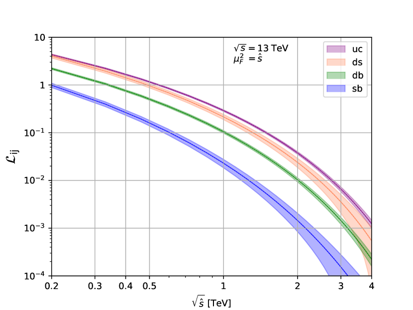
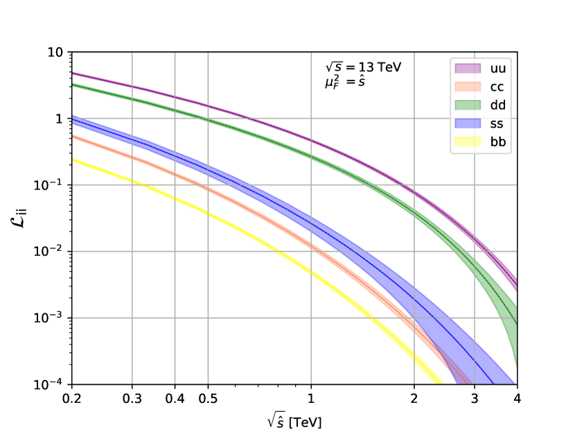
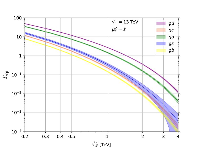
Figure 4: The parton luminosity functions (14) for different combinations of partons. The upper left panel corresponds the flavor off-diagonal quark combinations and the upper right figure to flavor diagonal quark combinations. The lower plot shows the combinations of quarks and gluons. We use the PDFset PDF4LHC15_nlo_mc Butterworth et al. (2016); Harland-Lang et al. (2015); Ball et al. (2015); Dulat et al. (2016) with the factorization scale $\mu_{F}=\sqrt{\hat{s}}$. Solid lines correspond to the central values and the envelope shows the $1\sigma$-ranges for the PDF uncertainties.

Note that the definition of the PLFs (14) differs from the one in Ref. Angelescu et al. (2020), since we group together $q\bar{q}^{\prime}$ and $q^{\prime}\bar{q}$, since this definition is manifestly symmetric under $i\Leftrightarrow j$ and we extend the definition to include gluons. On the other hand for diagonal quark combinations equation (14) is identical with the one in Ref. Angelescu et al. (2020) and, moreover, only slight differences for off-diagonal couplings are visible. Furthermore the total cross section is identical, regardless of the definition, since the sum over all possible inital partons has to be considered.

The partonic cross sections are worked out analytically, to understand the shape and relative size of the NP contributions, as well as to validate the simulation based on tools decribed in Sec. IV. This framework generalizes the parametrization used in Lam and Tung (1978) and can be extended to other processes, such as $e^{+}e^{-}\rightarrow\text{Hadrons},e^{+}p\rightarrow X,pp\rightarrow\ell^{-}\ell^{+}+X$. Details are provided in App. B.

III.2 Shapes of SMEFT-distributions

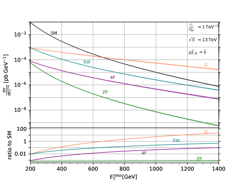
Figure 5: $E_{T}^{miss}$ distributions at LO for $pp\rightarrow\nu\bar{\nu}+X$ in the SM (black) and insertions of FCNC gluon dipole ($G$, orange), electroweak dipole ($EW$, petrol), four-fermion ($4F$, pink) and $Z$-penguin ($ZP$, green) operators inducing $uc$-transitions. NP effects are for $\Lambda_{NP}=$1\text{\,}\mathrm{TeV}$$ and effective WCs fixed to $C^{i}_{uc}=1$ and all others to zero, to illustrate the relative shapes and reach of the NP contributions, see text. We use the PDFset PDF4LHC15_nlo_mc Butterworth et al. (2016); Harland-Lang et al. (2015); Ball et al. (2015); Dulat et al. (2016) and $\mu_{F},\mu_{R}=\sqrt{\hat{s}}$. PDF uncertainties are included, yet very small.

We show in Fig. 5 the LO $E_{T}^{miss}$ differential cross sections after PLF-folding for the SM and exemplarily for operator insertions with $uc$ FCNCs, see also footnote 2. Fig. 5 illustrates the shapes and hierarchies between different operator insertions. The effect from flavor can be inferred from the hierarchies of the PLFs, shown in Fig. 4. The lower part of Fig. 5 gives the ratio of NP spectra to the SM one, displaying the relative energy growth of the different operators. Since $\Lambda_{NP}/\sqrt{C_{uc}^{i}}=$1\text{\,}\mathrm{TeV}$$ is a rather low value, this should be considered as an illustration rather than the typical NP benchmark.

Since the $Z$-penguins ($ZP$, green) have the same Dirac-structure as the SM (black), the shapes of their $P_{T}$-distributions are identical. The other contributions experience further energy-enhancements. Recall that both quark-antiquark annihilation as well as quark-gluon fusion diagrams contribute, which are folded with different PLFs. At parton level, quark-antiquark fusion has always the larger contributions except for the gluon dipoles, for which they are of similar size. On the other hand, the $qg$-PLFs are about one order of magnitude larger. After folding, the largest impact has the gluon dipole ($G$, orange), followed by the EW dipole ($EW$, petrol) and four-fermion operators ($4F$, pink).

The shapes and hierarchies in Fig. 5 can be understood from the differential partonic cross sections, here for $q_{i}g\rightarrow\nu\bar{\nu}q_{j}$. In the high energy limit, $M_{Z},v\ll P_{T}\sim\sqrt{\hat{s}}/2$, they can be written as

$$\frac{\mathrm{d}\hat{\sigma}_{SM}(q_{i}g\rightarrow\nu\bar{\nu}q_{j})}{\mathrm{d}P_{T}} \approx\frac{\alpha_{s}\text{Br}(Z\rightarrow\nu\bar{\nu})\left({\epsilon_{L}^{i,j}}^{2}+{\epsilon_{R}^{i,j}}^{2}\right)}{12\sqrt{2}}\frac{1}{\hat{s}^{3/2}}\frac{x^{2}+4}{x\sqrt{1-x^{2}}}\,,$$ (15)

$$\frac{\mathrm{d}\hat{\sigma}_{ZP}(q_{i}g\rightarrow\nu\bar{\nu}q_{j})}{\mathrm{d}P_{T}} \approx\frac{\alpha_{s}{C^{ZP}_{ij}}^{2}\text{Br}\left(Z\rightarrow\nu\bar{\nu}\right)}{24}\frac{M_{Z}^{2}v^{2}}{\Lambda_{NP}^{4}}\frac{1}{\hat{s}^{3/2}}\frac{x^{2}+4}{x\sqrt{1-x^{2}}}\,,$$ (16)

$$\frac{\mathrm{d}\hat{\sigma}_{4F}(q_{i}g\rightarrow\nu\bar{\nu}q_{j})}{\mathrm{d}P_{T}} \approx\frac{5\alpha_{s}{C^{4F}_{ij}}^{2}}{432\sqrt{2}\pi^{2}}\frac{1}{\Lambda_{NP}^{4}}\sqrt{\hat{s}}(1-x)^{3/2}\,,$$ (17)

$$\frac{\mathrm{d}\hat{\sigma}_{EW}(q_{i}g\rightarrow\nu\bar{\nu}q_{j})}{\mathrm{d}P_{T}} \approx\frac{\alpha_{s}(C^{EW}_{ij})^{2}\text{Br}\left(Z\rightarrow\nu\bar{\nu}\right)}{6\sqrt{2}}\frac{v^{2}}{\Lambda_{NP}^{4}}\frac{1}{\sqrt{\hat{s}}}\frac{x}{\sqrt{1-x^{2}}}\,,$$ (18)

$$\frac{\mathrm{d}\hat{\sigma}_{G}(q_{i}g\rightarrow\nu\bar{\nu}q_{j})}{\mathrm{d}P_{T}} \approx\frac{{C^{G}_{ij}}^{2}\text{Br}\left(Z\rightarrow\nu\bar{\nu}\right)\left(\epsilon_{L}^{i,j}-{\epsilon_{R}^{i,j}}\right)^{2}v^{2}}{96\pi M_{Z}^{2}}\frac{1}{\Lambda_{NP}^{4}}\sqrt{\hat{s}}\frac{x}{\sqrt{1-x^{2}}}\,,$$

$$=\frac{{C^{G}_{ij}}^{2}\text{Br}\left(Z\rightarrow\nu\bar{\nu}\right)}{96\pi}\frac{1}{\Lambda_{NP}^{4}}\sqrt{\hat{s}}\frac{x}{\sqrt{1-x^{2}}}\,,$$ (19)

where $x=2P_{T}\,/\sqrt{\hat{s}}$, $\text{Br}(Z\rightarrow\nu\bar{\nu})\simeq 20\%$ Schael et al. (2006) is the SM branching ratio of the $Z$-boson to neutrinos, and $\epsilon_{L(R)}^{i,j}$ are the SM $Z$-couplings to left-(right-) handed quarks (83). Here, we employed the narrow-width approximation, but used the full expressions in the numerical analysis. The energy-dependence of the quark-antiquark fusion processes is similar, and given in App. B. Due to the larger PLFs the hadronic $P_{T}$-spectra are dominated by quark-gluon fusion.

Comparing the differential cross section of the $Z$-penguins (16) with the SM one, (15), which drops as $1/\hat{s}^{3/2}$, one observes that the former is suppressed by $\sim v^{4}/\Lambda_{NP}^{4}$. On the other hand, the EW-dipoles (18) are lesser suppressed by the NP scale, and receive partial energy enhancement relative to the SM as $\sim v^{2}\hat{s}/\Lambda_{NP}^{4}$. Both four-fermion (17) and gluon dipole operators (19) are fully energy-enhanced relative to the SM, $\sim\hat{s}^{2}/\Lambda_{NP}^{4}$. All but the four-fermion insertion involve the $Z$-resonance to produce dineutrinos, therefore only the 4F-process is a genuine $(2\rightarrow 3)$-process, and has stronger phase space suppression than the others including the SM.

IV Recast of the experimental analysis

In this section the simulation chain used for the recast of the experimental analysis Aad et al. (2021a) is described. First the feynman rules for the process are exported as an UFO model, which is then read in by MadGraph5_aMC@NLO Frederix et al. (2018). For the SM calculations the "sm" UFO file is used, while the SMEFT contributions are based on the UFO model SMEFTsim_general_MwScheme_UFO Brivio (2021). Using MadGraph5_aMC@NLO statistical significant events samples of $pp\rightarrow\nu\bar{\nu}+X$ are generated. The resulting samples are showered and hadronized using Pythia8 Bierlich et al. (2022) and finally detector effects are estimated using Delphes3 de Favereau et al. (2014). For this the ATLAS Delphes card is used and final selection criteria are applied using ROOT. Jets are clustered with the anti-$k_{T}$ algorithm with a jet radius $\Delta R=0.4$ using the program fastJet Cacciari et al. (2012). The factorization and renormalization scales are chosen as $\mu_{R}=\mu_{F}=\frac{1}{2}\sum_{i}P_{T,i}$, where the sum is over all final states.

We recast the ATLAS analysis Aad et al. (2021a), which examines events with an energetic jet and missing transverse momentum. The dataset is based on Run II data and corresponds to an integrated luminosity $\mathcal{L}_{int}=$139\text{\,}\mathrm{fb}$^{-1}$ at a center-of-mass energy $\sqrt{s}=$13\text{\,}\mathrm{TeV}$$. First SM background samples are calculated and compared to the background analysis reported in Aad et al. (2021a). The results are reproduced to an accuracy of $$10\text{\,}\mathrm{\char 37\relax}$-$20\text{\,}\mathrm{\char 37\relax}$$. Subsequently the pure BSM contribution is computed for $C_{i}=1$ and then rescaled to obtain limits.

We also work out projections for the HL-LHC ($\mathcal{L}_{int}=$3000\text{\,}\mathrm{fb}$^{-1}$), assuming that data scales with the luminosity ratio, while all uncertainties scale with the square root of the luminosity ratio. These projections can be considered as rather conservative, since the HL-LHC will increase the center-of-mass energy to $\sqrt{s}=$14\text{\,}\mathrm{TeV}$$. This could lead to additional bins for high-$P_{T}$ in the tails of the distribution, that are currently not probed, however are expected to be most sensitive.

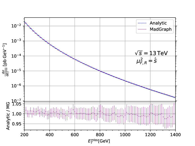
(a)

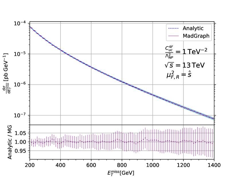
(b)

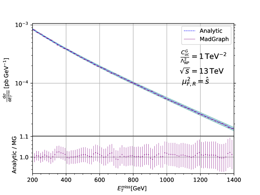
(c)

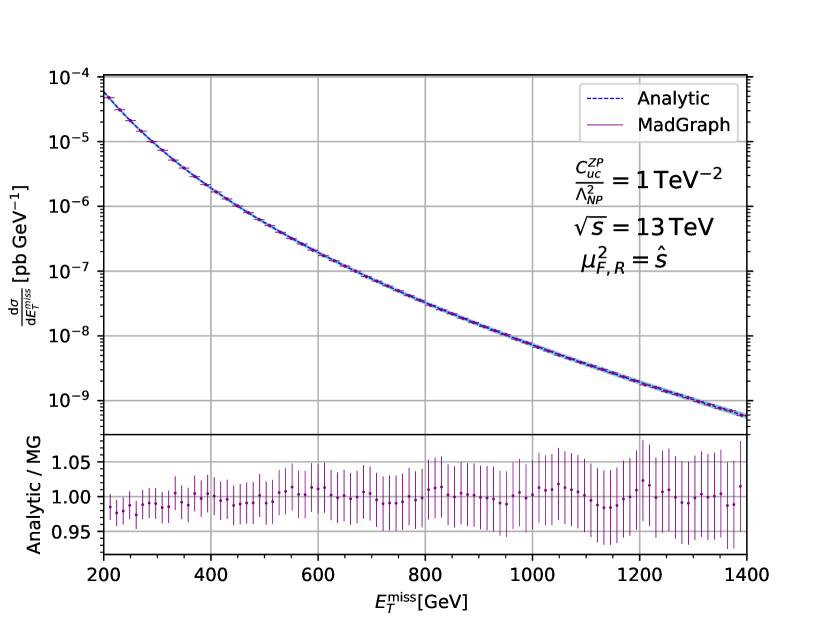
(d)

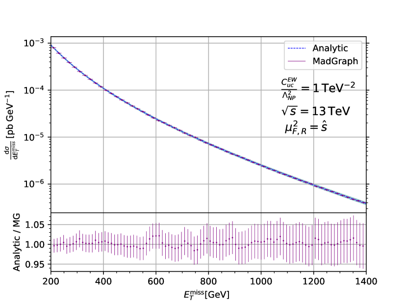
(e)

Figure 8: Analytical results from App. B, compared with the MadGraph5_aMC@NLO Frederix et al. (2018) results using the UFO model SMEFTsim_general_MwScheme_UFO Brivio (2021). Shown are the SM prediction (a), as well as predictions for $C^{4F}_{uc}$ (b), $C^{G}_{uc}$ (c), $C^{ZP}_{uc}$ (d) and $C^{EW}_{uc}$ (e), see Secs. II.2,II.3 and II.4.

The constraints on the effective WCs are extracted using the CLs method Read (2002). These are computed using the framework pyhf Heinrich et al. and all WCs with $\text{CLs}<0.05$ are excluded. Systematic errors for the signal simulations are neglected. We validate our numerical simulation with a study of analytical properties, which is detailed in App. B. Missing energy spectra based on Madgraph and our analytical computation are compared in Fig. 8, and show very good agreement with each other. The input parameters for the analytical results are based on Ref. Workman et al. (2022). The results of the recast are presented in Sec. V.

V Constraining New Physics

We give the results of the SMEFT recast of the $pp\to\text{MET}+j$ search Aad et al. (2021a). The limits, presented in Sec. V.1, are obtained by switching on a single effective NP coupling, while setting all others to zero. For operators containing left-handed up-type (down-type) quarks we present limits in the up-mass (down-mass) basis. Our analysis also allows for an application to models with light right-handed neutrinos, discussed in Sec.V.2. In Sec V.3 we compare our constraints on semileptonic four-fermion operators with those from rare decays and Drell-Yan production. We make comments on dipole coefficients and compare available constraints in Sec. V.4.

V.1 Results for SMEFT operators

${ij}$	$C^{G}_{ij}$	$C^{EW}_{ij}$	$C^{4F}_{ij}$	$C^{ZP}_{ij}$
$uc$	$0.0077$($0.0059$)	$0.036$ ($0.029$)	$0.079$($0.060$)	$0.39$ ($0.30$)
$ds$	$0.011$ ($0.009$)	$0.051$ ($0.040$)	$0.11$ ($0.09$)	$0.47$ ($0.34$)
$db$	$0.012$ ($0.010$)	$0.056$ ($0.043$)	$0.14$ ($0.10$)	$0.54$ ($0.38$)
$sb$	$0.026$ ($0.020$)	$0.12$ ($0.10$)	$0.37$ ($0.30$)	$1.07$ ($0.78$)

Table 2: The $95\%$ CL-limits on effective gluon dipole WCs (3), electroweak dipole WCs (4), four-fermion WCs (2), and $Z$-penguins (10) for off-diagonal quark flavor combinations $i\neq j$ and a NP scale $\Lambda_{NP}=$1\text{\,}\mathrm{TeV}$$ from the ATLAS search Aad et al. (2021a). Values in parentheses correspond to projections ($\mathcal{L}_{int}=$3000\text{\,}\mathrm{fb}$^{-1}$) assuming naive statistical scaling.

In Table 2 we give the bounds on the effective coefficients and projections for the high-luminosity upgrade for the FCNC semileptonic four-fermion, gluonic dipole, EW dipole operators and $Z$-penguin operators. As the parton luminosities are the largest for $uc$, followed by $ds$, $db$ and $sb$, see Fig. 4, the bounds are strongest for $uc$, followed by $ds$, $db$ and $sb$. Limits can be translated into a NP scale $\Lambda_{NP}$ that can be probed, shown in Fig. 6 with the highest reach necessarily in $uc$-transitions. Bounds on gluonic dipole operators are the strongest, $11.4\text{\,}\mathrm{TeV}$, followed by the EW dipole operators $5.6\text{\,}\mathrm{TeV}$, the four-fermion operators $3.6\text{\,}\mathrm{TeV}$, and the $Z$-penguin operators $1.6\text{\,}\mathrm{TeV}$, consistent with the shapes and enhancements discussed in Sec. III.2.

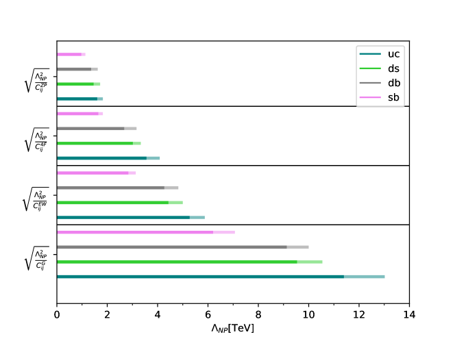
Figure 6: NP scales probed in $pp\to\text{MET}+j$ via FCNC transitions corresponding to the limits in Table 2. The vertical axis shows, from top to bottom and with increasing relative reach, the limits from $Z$-penguin, four-fermion, electroweak and gluon dipole insertions for the quark flavor changes $sb$ (pink), $db$ (brown), $ds$ (green) and $uc$ (dark green).

In Table 3 we present limits on flavor conserving dipole operators. Note, their interference with the SM is chirality suppressed, i.e., involves a fermion mass, which we safely neglect.

$ii$	$C^{G}_{ii}/\sqrt{2}$	$C^{EW}_{ii}/\sqrt{2}$
$uu$	$0.0051$($0.0039$)	$0.023$($0.018$)
$dd$	$0.0079$($0.0062$)	$0.034$($0.027$)
$ss$	$0.023$($0.018$)	$0.091$($0.075$)
$cc$	$0.028$($0.023$)	$0.11$($0.09$)
$bb$	$0.038$($0.031$)	$0.17$($0.14$)

Table 3: The $95\%$ CL-limits on effective gluon dipole WCs (3) and electroweak $Z$-dipole WCs (4) quark flavor conserving combinations, see Table 2. The factor $1/\sqrt{2}$ accounts for the fact that the Wilson coefficients for the chirality-flipped insertions coincide for diagonal flavors.

The bounds for the diagonal couplings also follow the luminosities, that is, $uu$ has the strongest bound, probing scales up to 14 TeV, followed by $dd$, $ss$, $cc$ and $bb$.

Increasing the luminosity to $$3000\text{\,}\mathrm{fb}$^{-1}$ would tighten the limits in Tables 2, 3 by $(70-80)\%$.

V.2 Limits on light right-handed neutrinos

Light right-handed neutrinos $N$, which are singlets of the SM, can be added to the dimension-six SMEFT-lagrangian as

$$\mathcal{L}^{6}_{\text{SMEFT}+N} \supset\frac{C_{Nq,klij}}{\Lambda_{NP}^{2}}\left(\bar{N}_{k}\gamma_{\mu}N_{l}\right)\left(\bar{q}_{i}\gamma^{\mu}q_{j}\right)+\frac{C_{Nu,klij}}{\Lambda_{NP}^{2}}\left(\bar{N}_{k}\gamma_{\mu}N_{l}\right)\left(\bar{u}_{i}\gamma^{\mu}u_{j}\right)$$ (20)

$$+\frac{C_{Nd,klij}}{\Lambda_{NP}^{2}}\left(\bar{N}_{k}\gamma_{\mu}N_{l}\right)\left(\bar{d}_{i}\gamma^{\mu}d_{j}\right)$$

where $k,l$ are flavor indices of the $N$’s. In principle, the numbers of flavors for the singlet neutrinos can be different from the left-handed ones. Feynman diagrams contributing to $pp\to\text{MET}+j$ are given in Fig. 1 with the $\nu$’s replaced by the $N$’s. Assuming $Z$-decays to invisibles to be SM-like, there is no contribution from the singlet neutrinos via dipole or penguins operators. Note that further (pseudo-)scalar four-fermion operators with both a left-handed and a right-handed neutrino exist but these are not considered in this work. The Wilson coefficients for the singlets $C_{Nq},C_{Nu},C_{Nd}$ can be constrained just like the ones involving left-handed neutrinos using (2) as

$$C^{4F+N}_{ij}=\sqrt{|C^{4F}_{ij}|^{2}+\sum_{k,l}|C_{Nq,klij}|^{2}+|C_{Nu/d,klij}|^{2}}\,.$$ (21)

Therefore, upper limits on $C^{4F}_{ij}$ given in Table 2 apply to $C^{4F+N}_{ij}$.

V.3 Comparison of bounds on four-fermion operators

We compare the limits on four-fermion operators $C_{ij}^{4F}$ from $pp\to\text{MET}+j$ given in Table 2 to existing ones from Drell-Yan production of charged leptons and rare decays of kaons, charm and beauty mesons. We make use of $SU(2)_{L}$-links, that enable a representation of dineutrino limits in terms of left-handed dilepton coefficients $\mathcal{K}_{L,R}^{qq^{\prime}\ell\ell^{\prime}}$, where the subscript indicates left ($L$), right $(R$)-chiral quark $|\Delta q|=|\Delta q^{\prime}|=1$ FCNCs. Limits on up-type FCNCs with dineutrinos imply limits on right-handed up-type currents and left-handed down-type currents with charged leptons, and vice versa. We follow closely Bause et al. (2022), and give details on the SMEFT-WET matching and $SU(2)_{L}$-machinery in App. A.1. Coefficients for lepton flavor violating (LFV) transitions are given as charge-summed

$$\overline{\mathcal{K}^{\ell+\ell^{\prime}-}_{L,R}}=\sqrt{|\mathcal{K}_{L,R}^{\ell+\ell^{\prime}-}|^{2}+|\mathcal{K}_{L,R}^{\ell-\ell^{\prime}+}|^{2}}\,.$$

Constraints on four-fermion operators are summarized in Tables 4, 5, 6 and 7 for $uc$, $ds$, $db$ and $sb$, respectively. Top quark couplings can as well be constrained by $SU(2)_{L}$ and $b$-physics data, resulting limits are shown in Tables 8 and 9 for $tu$ and $tc$ couplings, respectively. Note, the tables are in parts adopted from Bause et al. (2022), with updates from Grunwald et al. (2023). The novel entries obtained in this work are in the last rows, from the process $pp\to\nu\bar{\nu}+X$. We discuss the impact on the individual sectors below.

V.3.1 $cu\ell\ell^{\prime}$-transitions

The best limits on $\mathcal{K}^{cu\ell\ell^{\prime}}_{L}$ are from kaon decays, $K\to\pi\nu\bar{\nu}$, about two orders of magnitude stronger than the other $cu\ell\ell^{\prime}$-ones. The best limits on $\mathcal{K}^{cu\ell\ell^{\prime}}_{R}$ are from $pp\to\nu\bar{\nu}+X$ if taus are involved: $\ell\ell^{\prime}=\tau\tau,e\tau,\mu\tau$. For the other lepton flavors they are competitive with Drell-Yan and rare $D$-decays, where the latter dominates the $\mathcal{K}^{cu\mu\mu}_{R}$- limit.

Process	WC	$ee$	$\mu\mu$	$\tau\tau$	$e\mu$	$e\tau$	$\mu\tau$
$pp\rightarrow\ell^{+}\ell^{-}\qquad$	$\mathcal{K}^{cu\ell\ell^{\prime}}_{L,R}\qquad$	2.9	1.6	5.6	1.6	4.7	5.1
$D\rightarrow\ell^{+}\ell^{-}+\pi$	$\mathcal{K}^{cu\ell\ell^{\prime}}_{L,R}\qquad$	4.0	0.9	-	2.2	-	-
$K\rightarrow\nu\bar{\nu}\quad+\pi$	$\mathcal{K}^{cu\ell\ell^{\prime}}_{L}\cdot${10}^{2}$$	$[-1.9,0.7]$	$[-1.9,0.7]$	$[-1.9,0.7]$	$1.1$	$1.1$	$1.1$
$pp\rightarrow\nu\bar{\nu}\quad+X$	$\mathcal{K}^{cu\ell\ell^{\prime}}_{L}\qquad$	5.7 (4.6)	5.7 (4.6)	5.7 (4.6)	4.1 (3.3)	4.1 (3.3)	4.1 (3.3)
$pp\rightarrow\nu\bar{\nu}\quad+X$	$\mathcal{K}^{cu\ell\ell^{\prime}}_{R}\qquad$	4.1 (3.3)	4.1 (3.3)	4.2 (3.3)	2.9 (2.2)	2.9 (2.2)	2.9 (2.2)

Table 4: Limits on $cu\ell\ell^{\prime}$ WCs. The first three rows are taken from Bause et al. (2022), while the ones from $pp\to\nu\bar{\nu}+X$ are based on table 2, with projections for $$3000\text{\,}\mathrm{fb}$^{-1}$ in parentheses, using $SU(2)$  Bause et al. (2022). LFV-bounds are given as flavor-summed.

V.3.2 $sd\ell\ell^{\prime}$-transitions

The best limits on $\mathcal{K}^{sd\ell\ell^{\prime}}_{R}$ (from $K\to\pi\nu\bar{\nu}$) and $\mathcal{K}^{sd\ell\ell^{\prime}}_{L}$ for $\ell\ell^{\prime}=ee,\mu\mu,e\mu$, are from rare $K$-decays, about two orders of magnitude stronger than all others. The best limits on $\mathcal{K}^{sd\ell\ell^{\prime}}_{L}$ with taus, $\ell\ell^{\prime}=\tau\tau,e\tau,\mu\tau$ are from $pp\to\nu\bar{\nu}+X$. Dilepton Drell-Yan (first row) and $\text{MET}+j$ imits (last two rows) are of similar size.

Process	WC	$ee$	$\mu\mu$	$\tau\tau$	$e\mu$	$e\tau$	$\mu\tau$
$pp\rightarrow\ell^{+}\ell^{-}\qquad$	$\mathcal{K}^{sd\ell\ell^{\prime}}_{L,R}\qquad$	3.8	2.3	5.37	2.0	6.1	6.6
$K\rightarrow\ell^{+}\ell^{-}+\pi$	$\mathcal{K}^{sd\ell\ell^{\prime}}_{L,R}\cdot${10}^{2}$$	$5$	$1.6$	-	$6.6\text{\times}{10}^{-2}$	-	-
$K\rightarrow\nu\bar{\nu}\quad+\pi$	$\mathcal{K}^{sd\ell\ell^{\prime}}_{R}\cdot${10}^{2}$$	[-1.9,0.7]	[-1.9,0.7]	[-1.9,0.7]	$1.1$	$1.1$	$1.1$
$pp\rightarrow\nu\bar{\nu}\quad+X$	$\mathcal{K}^{sd\ell\ell^{\prime}}_{L}\qquad$	4.1 (3.3)	4.1 (3.3)	4.1 (3.3)	2.9 (2.2)	2.9 (2.2)	2.9 (2.2)
$pp\rightarrow\nu\bar{\nu}\quad+X$	$\mathcal{K}^{sd\ell\ell^{\prime}}_{R}\qquad$	5.7 (4.6)	5.7 (4.6)	5.7 (4.6)	4.1 (3.3)	4.1 (3.3)	4.1 (3.3)

Table 5: Limits on $sd\ell\ell^{\prime}$ WCs. The first row is based on Grunwald et al. (2023), while the second and third row are taken from Bause et al. (2022). See table 4.

V.3.3 $bq\ell\ell^{\prime}$-transitions

For WCs involving $b$-quarks, the $pp\rightarrow\nu\bar{\nu}+X$ analysis (last row of tables 6 and 7) can only provide constraints on right-chiral WCs $\mathcal{K}^{bq\ell\ell^{\prime}}_{R}$. For both $q=d,s$ FCNCs the corresponding limits from rare $B$-meson decays into invisibles (second to last rows) are stronger, and more so for $b\to s$, because the PLF is smaller and, on the other hand, the $b\to s\nu\bar{\nu}$ branching ratios are larger than the ones for $b\to d$. When taus are not involved, precision studies of semileptonic rare $B$-decays give more than an order of magnitude better bounds than from high $p_{T}$-studies.

Process	WC	$ee$	$\mu\mu$	$\tau\tau$	$e\mu$	$e\tau$	$\mu\tau$
$pp\rightarrow\ell^{+}\ell^{-}\qquad$	$\mathcal{K}^{bd\ell\ell^{\prime}}_{L,R}$	5.4	3.2	6.5	3.1	9.6	11
$B\rightarrow\ell^{+}\ell^{-}+X$	$\mathcal{K}^{bd\ell\ell^{\prime}}_{R}$	0.09	[-0.03, 0.03]	21	$0.2$	3.4	2.4
$B\rightarrow\ell^{+}\ell^{-}+X$	$\mathcal{K}^{bd\ell\ell^{\prime}}_{L}$	0.09	[-0.07,-0.02]	21	$0.2$	3.4	2.4
$B\rightarrow\nu\bar{\nu}+(\pi,\rho)$	$\mathcal{K}^{bd\ell\ell^{\prime}}_{R}$	1.8	1.8	1.8	2.5	2.5	2.5
$pp\rightarrow\nu\bar{\nu}\quad+X$	$\mathcal{K}^{bd\ell\ell^{\prime}}_{R}$	7.3(5.2)	7.3(5.2)	7.3(5.2)	5.2(3.7)	5.2(3.7)	5.2(3.7)

Table 6: Constraints on $bd\ell\ell^{\prime}$ WCs. The first row is based on Grunwald et al. (2023), while the second, third and fourth row are taken from Bause et al. (2022). See table 4.

Process	WC	$ee$	$\mu\mu$	$\tau\tau$	$e\mu$	$e\tau$	$\mu\tau$
$pp\rightarrow\ell^{+}\ell^{-}\qquad$	$\mathcal{K}^{bs\ell\ell^{\prime}}_{L,R}$	15	8.9	17	8.0	27	30
$B\rightarrow\ell^{+}\ell^{-}+X$	$\mathcal{K}^{bs\ell\ell^{\prime}}_{R}$	0.04	[-0.03,-0.01]	32	$0.1$	2.8	3.4
$B\rightarrow\ell^{+}\ell^{-}+X$	$\mathcal{K}^{bs\ell\ell^{\prime}}_{L}$	0.04	[-0.07,-0.04]	32	$0.1$	2.8	3.4
$B\rightarrow\nu\bar{\nu}\quad+K^{(*)}$	$\mathcal{K}^{bs\ell\ell^{\prime}}_{R}$	1.4	1.4	1.4	1.8	1.8	1.8
$pp\rightarrow\nu\bar{\nu}\quad+X$	$\mathcal{K}^{bs\ell\ell^{\prime}}_{R}$	19.3(15.3)	19.3(15.3)	19.3(15.3)	13.6(11.1)	13.6(11.1)	13.6(11.1)

Table 7: Limits on $bs\ell\ell^{\prime}$ WCs. The first row is based on Grunwald et al. (2023), while the second, third and fourth row are taken from Bause et al. (2022). See table 4.

V.3.4 $tq\ell\ell^{\prime}$-transitions

For FCNCs involving $t$-quarks, the $pp\rightarrow\nu\bar{\nu}+X$ analysis (last row) can only constrain left-chiral WCs $\mathcal{K}^{tq\ell\ell^{\prime}}_{L}$ (last rows tables 8 and 9). For both $ut$ and $ct$ FCNCs the corresponding $SU(2)$-limits from rare $B$-meson decays into invisibles (second rows) are stronger, and more so for $t\to c$ than for $t\to u$ due to effects already discussed for $bq\ell\ell^{\prime}$-transitions. To derive limits on $\mathcal{K}^{tq\ell\ell^{\prime}}_{R}$ one would need top-physics data, which would also constrain left-chiral $b$-quark couplings.

Process	WC	$ee$	$\mu\mu$	$\tau\tau$	$e\mu$	$e\tau$	$\mu\tau$
$t\>\>\rightarrow\ell^{+}\ell^{-}u$	$\mathcal{K}^{tu\ell\ell^{\prime}}_{L,R}$	$\sim 200$	$\sim 200$	n.a.	12	136	136
$B\>\rightarrow\nu\bar{\nu}+(\pi,\rho)$	$\mathcal{K}^{tu\ell\ell^{\prime}}_{L}$	[-1.6,1.8]	[-1.6,1.8]	[-1.6,1.8]	2.4	2.4	2.4
$pp\rightarrow\nu\bar{\nu}+X$	$\mathcal{K}^{tu\ell\ell^{\prime}}_{L}$	7.3(5.2)	7.3(5.2)	7.3(5.2)	5.2(3.7)	5.2(3.7)	5.2(3.7)

Table 8: Limits on $tu\ell\ell^{\prime}$ WCs. The first two rows are taken from Bause et al. (2022). See table 4.

Process	WC	ee	$\mu\mu$	$\tau\tau$	$e\mu$	$e\tau$	$\mu\tau$
$t\rightarrow\ell^{+}\ell^{-}c$	$\mathcal{K}^{tc\ell\ell^{\prime}}_{L,R}$	$\sim 200$	$\sim 200$	n.a.	36	136	136
$B\rightarrow\nu\bar{\nu}+K^{(*)}$	$\mathcal{K}^{tc\ell\ell^{\prime}}_{L}$	[-1.9,0.9]	[-1.9,0.9]	[-1.9,0.9]	1.8	1.8	1.8
$pp\rightarrow\nu\bar{\nu}\>\>\>+X$	$\mathcal{K}^{tc\ell\ell^{\prime}}_{L}$	19.3(15.3)	19.3(15.3)	19.3(15.3)	13.6(11.1)	13.6(11.1)	13.6(11.1)

Table 9: Limits on $tc\ell\ell^{\prime}$ WCs. The first two rows are taken from Bause et al. (2022). See table 4.

V.3.5 Synopsis four-fermion bounds

The constraints derived in this work from $pp\rightarrow\nu\bar{\nu}+X$ give the presently strongest limits on left-handed $|\Delta s|=|\Delta d|=1$ FCNCs and right-handed $|\Delta c|=|\Delta u|=1$ FCNCs in couplings with taus involved, that is, for $\ell\ell^{\prime}=\tau\tau,e\tau,\mu\tau$ operators. All other cases in the first two generations of quarks are dominated by bounds from rare kaon decays, see Tables 4, 5. For other couplings, $pp\rightarrow\nu\bar{\nu}+X$ limits are comparable to those from Drell-Yan or rare charm decays. Dineutrino rare $B$-decays, however, provide stronger constraints. The novel limits are however also interesting as they are complementary and probe various theoretical and experimental systematics. We look forward to improved analyses of MET plus jet.

V.4 Comparison of bounds on dipole operators

The limits on the gluon dipole coefficients given in Table 3 improve on previous collider studies, here given for $\Lambda_{NP}=$1\text{\,}\mathrm{TeV}$$ Haisch and Koole (2021)

$$C_{uG,cc},C_{dG,bb}\lesssim 7~{}~{}(\text{dijet angular distribution}),\quad C_{dG,bb}\lesssim 0.40~{}~{}(\text{$b$-jets})$$ (22)

by two orders of magnitude for $cc$ and one for $bb$. For completeness, a fit to top-observables obtains constraints on the dipole couplings (for $\Lambda_{NP}=$1\text{\,}\mathrm{TeV}$$) as Grunwald et al. (2023)

$$C_{uG,tt}\lesssim 0.028,\quad C_{uB,tt}\lesssim 0.38,\quad C_{uW,tt}\lesssim 0.053\,.$$ (23)

For the discussion of constraints from low energy let us make some general remarks relevant for dipole operators. Firstly, severe constraints exist from CP-violating observables, notably electric dipole moments, but also CP-asymmetries, e.g. Haisch and Koole (2021); Fajfer et al. (2023) on the imaginary parts of the dipole coefficients. The $pp\to\nu\bar{\nu}X$ study, on the other hand, probes their modulus, hence is complementary. Secondly, our analysis probes the $Z$-direction of the electroweak coefficients $C_{u/dB}$ and $C_{u/dW}$ (4), while in low energy observables the photon-one is constrained. It is therefore useful to study in the future also $pp\to\nu\bar{\nu}+\gamma$, to access the photon-coupling directly, and to disentangle the hypercharge and $SU(2)_{L}$ contributions. In the following, we perform the comparison of constraints with only the gluon dipole operator $O_{u/dG}$ present at the high scale.

The dipole coefficients $C_{u/dX}$ ($X=G,W,B$) are subject to sizable effects from renormalization group running and mixing within SMEFT Alonso et al. (2014), and once matched onto the low energy theory, continue to do so. The main contributors in the low energy effective theory are the electromagnetic $C_{7}^{(\prime)}$ and gluonic $C_{8}^{(\prime)}$ dipole coefficients, see App A.2. As argued, from $pp\to\nu\bar{\nu}+X$ we do not probe the photon coupling and hence neglect contributions from the electroweak dipole operators at the high scale. On the other hand, $C_{7}^{(\prime)}$ is induced by running and mixing with the gluon dipole operator.

For the numerical evaluation of matching and running we employ the package wilson Aebischer et al. (2018). The input is provided by the SMEFT WCs Table 2 at $\Lambda_{NP}=$1\text{\,}\mathrm{TeV}$$. These bounds are evolved to the electroweak scale and matched onto the WET. The limits are further evolved within WET, down to the $b$-mass scale $\approx m_{b}$, where the results for $bs$ and $bd$ transitions are extracted. For charm-transitions, the $b$-quark is integrated out and the running is performed until the charm scale $\approx m_{c}$, where the bounds for $uc$-transitions are extracted. Quark masses are MS-bar masses at the corresponding mass scale. For $ds$-transitions, the charm-quark is integrated out and the running is performed until $\sim$1\text{\,}\mathrm{GeV}$$. The constraints on $C_{7},C^{\prime}_{7},C_{8},C^{\prime}_{8}$ are presented in Table 10.

$qq^{\prime}$	$\mu$	$|C_{7}|$	$|C_{7}^{\prime}|$	$|C_{8}|$	$|C_{8}^{\prime}|$
$uc$	$m_{c}$	$2.8$	$2.8$	$4.4$	$4.4$
$ds$	1 GeV	$7.1\text{\times}{10}^{4}$	$7.1\text{\times}{10}^{4}$	$2.2\text{\times}{10}^{5}$	$2.2\text{\times}{10}^{5}$
$db$	$m_{b}$	$240$	$240$	$48$	$49$
$sb$	$m_{b}$	$110$	$120$	$23$	$23$

Table 10: The $95\%$ CL upper limits on the WET coefficients at the scale $\mu$ from running and matching the gluonic dipole limits in SMEFT Table 2, see text. The photon dipole coefficients $C_{7}^{(\prime)}$ are induced by mixing with the gluon dipole operators.

Since the leading effect is QCD-running and QCD respects parity, the left-handed and right-handed sectors evolve independent from each other, and a splitting between $C_{7,8}$ and the chirality-flipped ones $C_{7,8}^{\prime}$ are only induced from SM-contributions and subdominant.

Due to the strong GIM-suppression the situation in charm is simpler than in the down-sector and the approximate formula is useful de Boer and Hiller (2017); Adolph et al. (2021)

$$C_{7}^{(\prime)}(m_{c})\simeq 0.4\big{(}C_{7}^{(\prime)}(\Lambda_{NP})-C_{8}^{(\prime)}(\Lambda_{NP})\big{)}\,,\qquad C_{8}^{(\prime)}(m_{c})\simeq 0.4C_{8}^{(\prime)}(\Lambda_{NP})\,.$$ (24)

It is valid to roughly 20% for $\Lambda_{NP}$ within 1-10 TeV, and for $C_{7}^{(\prime)}(\Lambda_{NP})=0$ consistent with Table 10 which is based on wilson. The branching ratios of $D^{0}\to\rho^{0}\gamma$ and $D\to\pi\mu^{+}\mu^{-}$ constrain $|C_{7}^{(\prime)}(m_{c})|\lesssim 0.3$ de Boer and Hiller (2017); Golz et al. (2021). Confronting this to the upper limit in Table 10 which stems from the gluon dipole constraint, we learn from Eq. (24) that there has to be a cancellation tuned to one order of magntitude between the photonic and gluonic contributions at high energies or the limits from $pp\to\nu\bar{\nu}+X$ on the gluon dipole operators are about one order of magnitude weaker than the ones from rare charm decays. This highlights the importance of collider studies including photons such as $pp\rightarrow\gamma+\nu\bar{\nu}$, which directly contributes to $C_{7}^{(\prime)}$. Constraints on the imaginary parts from low energy data are even stronger, $|\text{Im}(C_{8}^{(\prime)}(m_{c}))|\lesssim{\mathcal{O}}(0.1)$ from the CP-asymmetry $A_{CP}(D^{0}\rightarrow\rho^{0}\gamma)$ de Boer and Hiller (2017); Lyon and Zwicky (2022), and $|\text{Im}(C_{8}^{(\prime)}(m_{c}))|\lesssim${10}^{-3}$$ from CP-violation in hadronic 2-body $D^{0}$-decays, $\Delta A_{CP}$ de Boer and Hiller (2017); Giudice et al. (2012).

The limits from global fits of $B$-decay data on the gluon dipole coefficients are more than one order of magnitude stronger than the ones from $pp\rightarrow\nu\bar{\nu}+X$, $|C_{8}^{(\prime)}(m_{b})|\lesssim 1.6$ for $b\rightarrow s$ and $|C_{8}(m_{b})|\lesssim 3$ for $b\rightarrow d$ transitions. The corresponding constraints on the photon dipole are even stronger for $b\rightarrow s$ modes $|C_{7}^{(\prime)}(m_{b})|\lesssim 0.1$ and for $b\rightarrow d$-transitions $|C_{7}(m_{b})|\lesssim 2$ Bause et al. (2023); Mahmoudi et al. (2023). Again the bounds from Table 10 are several orders of magnitude weaker and are therefore not competitive.

For $s\rightarrow d$-transitions no comparable bounds on the modulus of the dipole couplings are found in the literature, but they are the least stringent ones in Table 10 and therefore are also not expected to be competitive.

VI Summary

We work out constraints on new physics in the SMEFT by recasting an ATLAS search Aad et al. (2021a) for large missing transverse energy and an energetic jet at the LHC. The limits are presented in Tables 2, 3, and given in terms of effective WCs of semileptonic four-fermion operators, gluon and electroweak dipole operators and $Z$-penguins. Performing an explicit analytical computation of partonic cross sections we show that all operators except the $Z$-penguins are energy-enhanced, see Sec. III.2. The gluon dipole operators have the highest sensitivity to NP and probe energy scales up to $14$ TeV (the $uu$-coupling). We also obtain significantly improved limits on $C_{uG,cc}$ and $C_{dG,bb}$ over previous collider ones. To disentangle the hypercharge from the $SU(2)_{L}$ contributions to the $Z$-dipole coefficients (4) study of $pp\rightarrow\nu\bar{\nu}+\gamma$ Aad et al. (2021b) is encouraged, which directly probes the orthogonal, radiative dipole operator. This would also benefit synergies between high-$P_{T}$ and low energy observables, as there is large mixing among all dipole operators.

The constraints on four-fermion operators from $pp\to\text{MET}+j$ are presently the strongest for left-handed $|\Delta s|=|\Delta d|=1$ FCNCs and right-handed $|\Delta c|=|\Delta u|=1$ FCNCs if taus are involved, that is, for $\ell\ell^{\prime}=\tau\tau,e\tau,\mu\tau$ operators. All other cases in the first-second generation of quarks are dominated by bounds from rare kaon decays, see Tables 4, 5. The bounds from $pp\rightarrow\nu\bar{\nu}+X$ are comparable to those from conventional Drell-Yan production, except for tau flavors for which the MET-ones are better. This can be understood by noting that in $pp\rightarrow\ell^{+}\ell^{\prime-}$ analyses the $\tau$-tagging is typically inferior to $e$- or $\mu$-tagging.

We also consider light right-handed neutrinos as contributors to missing energy, see Sec. V.2. Further invisible light states can be probed in $pp\to\text{MET}+jet$ which could complement more model-specific searches for dark sectors. Present limits from low energy precision studies in $K\to\pi\nu\bar{\nu}$ and $B\to K^{(*)}\nu\bar{\nu}$ and $B\to(\pi,\rho)\nu\bar{\nu}$ are superior to the current $\text{MET}+jet$ sensitivity. Limits on rare charm decays to invisibles are presently not competitive with other constraints Bause et al. (2021a), and would require an order of magnitude improvement of the limit on the $D\to\pi\nu\bar{\nu}$ branching ratio Ablikim et al. (2022).

In conclusion, the interpretation of $pp\to\text{MET}+jet$ provides new constraints, which are complementary to other searches from high and low energies, and allow for a wider range of new physics explorations. We look forward to further studies with invisibles.

Appendix A Weak Effective Theory

Below the electroweak scale the $W$-boson and all particles heavier can be integrated out to obtain an EFT for low energy processes. This allows the interpretation of the high $P_{T}$-constraints, with others coming from low energy observables, such as decays. The connection between SMEFT and WET is given by the matching at the EW scale $\mu_{EW}=$160\text{\,}\mathrm{GeV}$$. This matching procedure and the running between the different scales will be discussed in the following sections. At first, the subsectionA.1 focusses on semileptonic four-fermion operator, while the second subsection A.2 focusses on the matching as well as running of the dipole operators.

A.1 Semileptonic four-fermion operators

The effective Hamiltonians for four-fermion operators with two quarks ($i,j$) and two leptons ($k,l$) is given by

$$\mathcal{H}^{\nu\bar{\nu}}_{eff}=\frac{-4G_{F}}{\sqrt{2}}\frac{\alpha_{e}}{4\pi}\sum_{k}\mathcal{C}_{k}^{P_{ijkl}}Q_{n}^{ijkl}+\text{h.c.},$$ (25)

for two dineutrinos and

$$\mathcal{H}^{\ell^{-}\ell^{+}}_{eff}=\frac{-4G_{F}}{\sqrt{2}}\frac{\alpha_{e}}{4\pi}\sum_{k}\mathcal{K}_{k}^{P_{ijkl}}O_{k}^{ijkl}+\text{h.c.},$$ (26)

for charged leptons, see Bause et al. (2021b, 2022) to which we refer for details. The superscript $P=D,U$ refers to the down or up sector, $\alpha_{e}$ denotes the fine structure constant and $G_{F}$ fermi’s constant. The calligraphic WCs are given in the mass basis and can each be written as the sum

$$\mathcal{K}_{k}^{P_{ijkl}}=\mathcal{K}_{k,SM}^{P_{ijkl}}+\mathcal{K}_{k,NP}^{P_{ijkl}}\,,$$ (27)

$$\mathcal{C}_{k}^{P_{ijkl}}=\mathcal{C}_{k,SM}^{P_{ijkl}}+\mathcal{C}_{k,NP}^{P_{ijkl}}\,,$$ (28)

where the SM contributions can be found in Bause et al. (2021b). The derived bound in the SMEFT is matched onto the WET and contribute only to the NP part of equation (27). Explicitly,

$$C^{U_{ijkl}}_{L} =K^{D_{ijkl}}_{L}=\frac{2\pi v^{2}}{\alpha_{e}\Lambda_{NP}^{2}}\left(C^{(1)}_{lq_{klij}}+C^{(3)}_{lq_{klij}}\right)\,,$$ (29)

$$C^{D_{ijkl}}_{L} =K^{U_{ijkl}}_{L}=\frac{2\pi v^{2}}{\alpha_{e}\Lambda_{NP}^{2}}\left(C^{(1)}_{lq_{klpr}}-C^{(3)}_{lq_{ijpr}}\right)\,,$$

$$C^{U_{ijkl}}_{R} =K^{U_{ijkl}}_{R}=\frac{2\pi v^{2}}{\alpha_{e}\Lambda_{NP}^{2}}C_{lu_{klij}}\,,$$

$$C^{D_{ijkl}}_{R} =K^{D_{ijkl}}_{R}=\frac{2\pi v^{2}}{\alpha_{e}\Lambda_{NP}^{2}}C_{ld_{klij}}\,,$$

where the upright coefficients denote the WET WCs in the gauge basis, which are related by a rotation to the calligraphic WCs in equation (26) and (25). Note that the first equal sign connects charged dileptons couplings with the dineutrino couplings. These relations follow from the SU(2) structure of the SMEFT. For the right-chiral singlets, the relations are straightforward. The left-chiral doublets get a sign change between $C^{(1)}_{lq}$ and $C^{(3)}_{lq}$, which connects the different quark sectors, i.e. $D\Leftrightarrow U$ as seen in the first two lines of (29).
The rotation to the mass basis can be done using $4$ rotation matrices. In the quark sector there are two left-handed rotation matrices $V_{u,d}$ and two right-handed ones $U_{u,d}$, whereas there are only two rotation matrices for the lepton sector, which are given by $V_{l}$ and $V_{\nu}$. The rotations are then given by Bause et al. (2021b)

$$\mathcal{C}^{D}_{L} =V^{\dagger}_{\nu}V_{d}^{\dagger}C^{D}_{L}V_{d}V_{\nu}\,, \mathcal{C}_{R}^{D} =V_{\nu}^{\dagger}U_{d}^{\dagger}C_{R}^{D}U_{d}V_{\nu}\,,$$ (30)

$$\mathcal{K}^{D}_{L} =V_{l}^{\dagger}V_{d}^{\dagger}K_{L}^{D}V_{d}V_{l}\,, \mathcal{K}_{R}^{D} =V^{\dagger}_{l}U^{\dagger}_{d}K_{R}^{D}U_{d}V_{l}.$$ (31)

By summing over lepton flavors, expanding $V_{CKM}=V_{u}^{\dagger}V_{d}$ in $\lambda\sim 0.2$ and using the unitarity of the PMNS matrix $W=V^{\dagger}_{l}V_{\nu}$ leads to Bause et al. (2022)

$$\sum_{k,l=\nu_{e},\nu_{\mu},\nu_{\tau}}\left(|\mathcal{C}^{U_{ijkl}}_{L}|^{2}+|\mathcal{C}^{U_{ijkl}}_{R}|^{2}\right) =\sum_{l,k=e,\mu,\tau}\left(|\mathcal{K}^{D_{ijkl}}_{L}|^{2}+|\mathcal{K}^{U_{ijkl}}_{R}|^{2}\right)+\mathcal{O}(\lambda)$$ (32)

$$\sum_{k,l=\nu_{e},\nu_{\mu},\nu_{\tau}}\left(|\mathcal{C}^{D_{ijkl}}_{L}|^{2}+|\mathcal{C}^{D_{ijkl}}_{R}|^{2}\right) =\sum_{l,k=e,\mu,\tau}\left(|\mathcal{K}^{U_{ijkl}}_{L}|^{2}+|\mathcal{K}^{D_{ijkl}}_{R}|^{2}\right)+\mathcal{O}(\lambda)\,.$$ (33)

Using equations (29) and (32) and an explicit form for the effective WCs (2) can be found. For up-type quarks this reads

$${C^{4F}_{ij}}^{2}= \left(\frac{\alpha_{e}\Lambda_{NP}^{2}}{2\pi v^{2}}\right)^{2}\sum_{k,l=\nu_{e},\nu_{\mu},\nu_{\tau}}|\mathcal{C}^{U_{ijkl}}_{L}|^{2}+|\mathcal{C}^{U_{ijkl}}_{R}|^{2}$$ (34)

$$= \left(\frac{\alpha_{e}\Lambda_{NP}^{2}}{2\pi v^{2}}\right)^{2}\sum_{k,l=e,\mu,\tau}|\mathcal{K}^{D_{ijkl}}_{L}|^{2}+|\mathcal{K}^{U_{ijkl}}_{R}|^{2}+\mathcal{O}(\lambda),$$

whereas for down-type quarks

$${C^{4F}_{ij}}^{2}= \left(\frac{\alpha_{e}\Lambda_{NP}^{2}}{2\pi v^{2}}\right)^{2}\sum_{k,l=\nu_{e},\nu_{\mu},\nu_{\tau}}|\mathcal{C}^{D_{ijkl}}_{L}|^{2}+|\mathcal{C}^{D_{ijkl}}_{R}|^{2}$$ (35)

$$= \left(\frac{\alpha_{e}\Lambda_{NP}^{2}}{2\pi v^{2}}\right)^{2}\sum_{k,l=e,\mu,\tau}|\mathcal{K}^{U_{ijkl}}_{L}|^{2}+|\mathcal{K}^{D_{ijkl}}_{R}|^{2}+\mathcal{O}(\lambda).$$

A.2 Dipole operators

The effective Hamiltonian for dipole operator is given by

$$\mathcal{H}^{\text{Dip}}_{\text{eff}} =-\frac{4\,G_{F}}{\sqrt{2}}\left(C_{7}^{(\prime)}\mathcal{O}_{7}^{(\prime)}+C_{8}^{(\prime)}\mathcal{O}_{8}^{(\prime)}\right)\,,$$ (36)

where the electromagnetic and chromomagnetic operators for $q\to q^{\prime}$ transitions are given as

$$\mathcal{O}_{7}^{(\prime)} =\frac{e}{16\pi^{2}}m_{q}\lambda_{CKM}\left(\bar{q}^{\prime}_{L(R)}\sigma^{\mu\nu}F_{\mu\nu}q_{R(L)}\right)~{},$$ (37)

$$\mathcal{O}_{8}^{(\prime)} =\frac{g_{s}}{16\pi^{2}}m_{q}\lambda_{CKM}\left(\bar{q}^{\prime}_{L(R)}\sigma^{\mu\nu}T^{A}G^{A}_{\mu\nu}q_{R(L)}\right)~{},$$ (38)

where $m_{q}$ denotes the mass of the parent quark, $\sigma^{\mu\nu}=\frac{i}{2}[\gamma^{\mu},\gamma^{\nu}]$ and $e,g_{s}$ the electric and QCD coupling constants, respectively. The tree level matching is given by

$$C_{8}^{(\prime)} =\frac{8\pi^{2}v^{2}}{\Lambda^{2}y_{q}g_{s}\lambda_{CKM}}C_{uG\,,ij(ji)}\,,$$ (39)

$$C_{7}^{(\prime)} =\frac{8\pi^{2}v^{2}}{\Lambda^{2}y_{q}g_{s}\lambda_{CKM}}\left(\cos\theta_{W}C_{uB\,,ij(ji)}+\sin\theta_{W}C_{uW\,,ij(ji)}\right)\,,$$ (40)

where $y_{q}=m_{q}\sqrt{2}/v$, $\theta_{W}$ is the weak mixing angle and $\lambda_{CKM}=V_{tq^{\prime}}^{*}V_{q}$ is a CKM factor, that reads $\lambda_{CKM}=V_{tq^{\prime}}^{*}V_{tq}$ for down sector FCNCs $q\to q^{\prime}$, and $\lambda_{CKM}=1$ for $c\to u$ for easier comparison with the literature. Matching the chirality-flipped WC $C_{8}^{\prime}$ corresponds to flipping the quark flavor indices $i,j$ in the SMEFT WC.

Appendix B Perturbative calculation

The perturbative calculation is done for the LO contribution to the $P_{T}$-spectrum, which includes the processes $q_{i}(p_{1})\bar{q}_{j}(p_{2})\rightarrow\nu_{k}(k_{1})\bar{\nu}(k_{2})g(k_{3})$, $q_{i}(p_{1})g(p_{2})\rightarrow\nu_{k}(k_{1})\bar{\nu}_{l}(k_{2})q_{j}(k_{3})$ and $\bar{q}_{i}(p_{1})g(p_{2})\rightarrow\nu_{k}(k_{1})\bar{\nu}_{l}(k_{2})\bar{q}_{j}(k_{3})$. The last two processes are related through charge conjugation and the former two through crossing. The partonic mandelstam variables are defined as

$$\hat{s} =(p_{1}+p_{2})^{2}$$ (41)

$$\hat{t} =(p_{1}-k_{3})^{2}$$

$$\hat{u} =(p_{2}-k_{3})^{2}.$$

The collider variables are defined by

$$P_{T}^{2}=\frac{\hat{t}\hat{u}}{\hat{s}}$$ (42)

$$\cosh\eta=-\left(\frac{\hat{t}+\hat{u}}{2\sqrt{\hat{t}\hat{u}}}\right)$$

and $q^{2}$ is the invariant mass of the $\nu\bar{\nu}$-system $q^{\mu}=k_{1}^{\mu}+k_{2}^{\mu}$. We introduce a parametrization based on Ref. Lam and Tung (1978) and generalize it to include SMEFT effects, which manifestly separates the partonic kinematics, internal propagators and lepton kinematics. The partonic cross section can be written as

$$\mathrm{d}\hat{\sigma}=\frac{\mathcal{A}_{C}C_{F}C_{A}}{8(2\pi)^{5}}\frac{q^{2}}{\hat{s}}\sum_{\mathcal{I}_{1}\mathcal{I}_{2}}\hat{H}_{\mu\nu}^{\mathcal{I}_{1}\mathcal{I}_{2}}D^{\mathcal{I}_{1}\mathcal{I}_{2}}I^{\mu\nu}\mathrm{d}^{4}q$$ (43)

where $C_{F}=4/3,C_{A}=3$ and $\mathcal{A}_{C}$ is a color averaging factor, which reads $1/9$ for $q\bar{q}$ inital states and $1/24$ for $qg,\bar{q}g$ initial states. Furthermore, we define the multi index $\mathcal{I}=\{I,J,Y,Z\}$, which matches operator $\mathcal{I}\in\{\text{SM},\text{4F},\text{ZP},\text{EW},\text{G}\}$ with explicit vertices $I\in\{V,D\}$, for vector or dipole copulings, with chirality $Y\pm 1$ for the four-fermion or $q\bar{q}Z$-vertex and vertex $J\in\{V,D\}$ with chirality $Z=\pm 1$ for the $q\bar{q}g$-vertex. Formula (43) can be used to explicitly calculate all three partonic processes, however the focus is on the process $q_{i}(p_{1})\bar{q}_{j}(p_{2})\rightarrow\nu_{k}(k_{1})\bar{\nu}_{l}(k_{2})g(k_{3})$ in the following, to derive equation (43). The matrix element for the diagram can be written as

$$\mathcal{M}_{\mathcal{I}}=T^{A}J^{\mu}_{\mathcal{I}}C_{\mathcal{I}}J_{\mu}^{\text{lept}},$$ (44)

where the partonic current is defined as

$$J^{\mu}_{\mathcal{I}}=i\bar{v}(p_{2})\left(\Gamma^{\mu}_{IY}(q)\left(\frac{\not{p_{1}}-\not{k_{3}}}{\hat{t}}\right)\Gamma^{\nu}_{JZ}(k_{3})-\Gamma^{\nu}_{JZ}(k_{3})\left(\frac{\not{p_{2}}-\not{k_{3}}}{\hat{u}}\right)\Gamma^{\mu}_{IZ}(q)\right)u(p_{1})\epsilon^{*}_{\nu}(k_{3})$$ (45)

with vertices

$$\Gamma^{\mu}_{IY}(p)=\begin{cases}i\gamma^{\mu}\left(\frac{1+Y\gamma^{5}}{2}\right)&I=\text{V}\\ \sigma^{\mu\alpha}p_{\alpha}\left(\frac{1+Y\gamma^{5}}{2}\right)&I=\text{D}\end{cases}$$ (46)

The leptonic current is defined as

$$J_{\mu}^{\text{lept}}=i\bar{u}(k_{1})\gamma^{\mu}\frac{1-\gamma^{5}}{2}v(k_{2}),$$ (47)

which is left chiral, since only left handed neutrinos are considered in the final state. The coefficient function $\mathcal{C}_{\mathcal{I}}$ includes SM couplings, propagators and WCs, depending on the type of operator insertion $\mathcal{I}$. They are given in Sec.  B.2. The squared Matrix element (summed over all operators, final states and averaged over initial states) reads

$$|\overline{\mathcal{M}}|^{2} =\frac{\mathcal{A}_{C}}{4}\sum_{\mathcal{I}_{1}\mathcal{I}_{2},\text{spins}}\mathcal{M}_{\mathcal{I}_{1}}\mathcal{M}_{\mathcal{I}_{2}}^{*}$$ (48)

$$=\frac{\mathcal{A}_{C}}{4}\text{Tr}\{T^{A}T^{A}\}\sum_{\mathcal{I}_{1}\mathcal{I}_{2},\text{spins}}D^{\mathcal{I}_{1}\mathcal{I}_{2}}J^{\mu}_{\mathcal{I}_{1}}(J^{\nu}_{\mathcal{I}_{2}})^{\dagger}J_{\mu}^{\text{lept}}(J_{\nu}^{\text{lept}})^{\dagger}$$

where $\text{Tr}\{T^{A}T^{A}\}=C_{F}C_{A}$ and

$$D^{\mathcal{I}_{1}\mathcal{I}_{2}}=\mathcal{C}_{\mathcal{I}_{1}}\mathcal{C}_{\mathcal{I}_{2}}^{*},$$ (49)

where $\mathcal{C}_{\mathcal{I}_{1}}$ can be read of the feynman rules for the SMEFT Dedes et al. (2017) and are given in App.  B.2. The three-body phase space can be separated into

$$\mathrm{d}\Phi_{3}=\frac{1}{(2\pi)^{9}}\left(\delta^{4}\left(q-k_{2}-k_{3}\right)\frac{\mathrm{d}^{3}k_{1}}{2E_{1}}\frac{\mathrm{d}^{3}k_{2}}{2E_{2}}\right)\left(\delta^{4}\left(p_{1}+p_{2}-q-k_{3}\right)\frac{\mathrm{d}^{3}k_{3}}{2E_{3}}\right)\mathrm{d}^{4}q$$ (50)

which leads to the total partonic cross section

$$\mathrm{d}\hat{\sigma}=\frac{\mathcal{A}_{C}C_{F}C_{A}}{8(2\pi)^{5}}\frac{q^{2}}{\hat{s}}\sum_{\mathcal{I}_{1}\mathcal{I}_{2}}\hat{H}_{\mu\nu}^{\mathcal{I}_{1}\mathcal{I}_{2}}D^{\mathcal{I}_{1}\mathcal{I}_{2}}I^{\mu\nu}\mathrm{d}^{4}q.$$ (51)

The parton tensor is defined as

$$\hat{H}^{\mathcal{I}_{1}\mathcal{I}_{2}}_{\mu\nu}=\sum_{\text{spins}}\int\frac{\mathrm{d}^{3}k_{3}}{2E_{3}}\delta^{4}\left(p_{1}+p_{2}-q-k_{3}\right)J^{\mu}_{\mathcal{I}_{1}}\left(J^{\nu}_{\mathcal{I}_{2}}\right)^{\dagger}$$ (52)

while the lepton tensor can be calculated

$$I_{\mu\nu}= \int\frac{\mathrm{d}^{3}k_{1}}{2E_{1}}\frac{\mathrm{d}^{3}k_{2}}{2E_{2}}\frac{1}{q^{2}}\sum_{\text{spins}}J_{\mu}^{\text{lept}}(J_{\nu}^{\text{lept}})^{\dagger}$$ (53)

$$= \frac{\pi}{3}\left(-\eta^{\mu\nu}+\frac{q^{\mu}q^{\nu}}{q^{2}}\right).$$

The introduced separation in equation 43 is useful, since all relevant insertion of SMEFT operators are included fully in the partonic part $\hat{H}^{\mathcal{I}_{1}\mathcal{I}_{2}}_{\mu\nu}$, which in the end has to be contracted with the lepton tensor to produce the final cross section. Therefore, it is useful to further analyse the properties, which have been worked out in reference Lam and Tung (1978) for the hadronic counter part. This leads to the parametrization

$$\hat{H}^{\mathcal{I}_{1}\mathcal{I}_{2}}_{\mu\nu}= \delta(\hat{s}+\hat{t}+\hat{u}-q^{2})\frac{E_{q}}{E_{3}}\bigg{\{}\eta^{\perp}_{\mu\nu}\hat{F}^{\mathcal{I}_{1}\mathcal{I}_{2}}_{1}(\hat{s},\hat{t},\hat{u})+\left(p^{\perp}_{1}+p^{\perp}_{2}\right)_{\mu}\left(p^{\perp}_{1}+p^{\perp}_{2}\right)_{\nu}\hat{F}^{\mathcal{I}_{1}\mathcal{I}_{2}}_{2}(\hat{s},\hat{t},\hat{u})$$ (54)

$$+p^{\perp}_{1\mu}p^{\perp}_{1\nu}\hat{F}^{\mathcal{I}_{1}\mathcal{I}_{2}}_{3}(\hat{s},\hat{t},\hat{u})+p^{\perp}_{2\mu}p^{\perp}_{2\nu}\hat{F}^{\mathcal{I}_{1}\mathcal{I}_{2}}_{4}(\hat{s},\hat{t},\hat{u})$$

$$+\left(\eta_{\mu\nu}-\frac{2}{\hat{s}}\left(p_{1\mu}p_{2\nu}+p_{1\nu}p_{2\mu}\right)\right)\hat{F}^{\mathcal{I}_{1}\mathcal{I}_{2}}_{5}(\hat{s},\hat{t},\hat{u})+q_{\mu}\text{ -terms}\bigg{\}},$$

where the energy momentum conserving $\delta$-function and a phase space factor have been factored. The lorentz structures are given by

$$\eta^{\perp}_{\mu\nu}=\eta_{\mu\nu}-\frac{q_{\mu}q_{\nu}}{q^{2}}$$

$$p^{\perp}_{i,\mu}=\eta_{\mu\nu}\frac{p^{\nu}_{i}}{\sqrt{\hat{s}}},$$

following Ref. Lam and Tung (1978). We assume $\hat{H}^{\mathcal{I}_{1}\mathcal{I}_{2}}_{\mu\nu}$ to be symmetric and ignore terms proportional to $q^{\mu}$, since $I^{\mu\nu}$ is manifestly symmetric, as well as $I^{\mu\nu}q_{\mu}=0$. The structure functions $F^{\mathcal{I}_{i}\mathcal{I}_{2}}_{1}(\hat{s},\hat{t},\hat{u})$ capture all relevant contributions as in reference Lam and Tung (1978). However, we need to include one additional piece, since the general current $J^{\mu}_{\mathcal{I}}$ is not conserved and therefore $\hat{H}^{\mathcal{I}_{1}\mathcal{I}_{2}}_{\mu\nu}q^{\mu}\neq 0$, which leads to the inclusion of $F^{\mathcal{I}_{1}\mathcal{I}_{2}}_{5}(\hat{s},\hat{t},\hat{u})$. The end result, which directly contributes to the total cross section is given by the contraction

$$\hat{H}^{\mathcal{I}_{1}\mathcal{I}_{2}}_{\mu\nu}I^{\mu\nu} =\delta(q^{2}-\hat{s}-\hat{t}-\hat{u})\frac{E_{q}}{E_{3}}\mathcal{F}^{\mathcal{I}_{1}\mathcal{I}_{2}}(\hat{s},\hat{t},\hat{u}),$$ (55)

where

$$\mathcal{F}^{\mathcal{I}_{1}\mathcal{I}_{2}}(\hat{s},\hat{t},\hat{u}) =\frac{\pi}{3}\bigg{(}-3F_{1}^{\mathcal{I}_{1}\mathcal{I}_{2}}(\hat{s},\hat{t},\hat{u})+\frac{1}{4\hat{s}(\hat{s}+\hat{t}+\hat{u})}\big{\{}(\hat{t}+\hat{u})^{2}F_{2}^{\mathcal{I}_{1}\mathcal{I}_{2}}(\hat{s},\hat{t},\hat{u})$$ (56)

$$+(\hat{t}+\hat{s})^{2}F_{3}^{\mathcal{I}_{1}\mathcal{I}_{2}}(\hat{s},\hat{t},\hat{u})$$

$$+(\hat{s}+\hat{u})^{2}F_{4}^{\mathcal{I}_{1}\mathcal{I}_{2}}(\hat{s},\hat{t},\hat{u})+(2\hat{s}(\hat{s}+\hat{t}+\hat{u})-\hat{u}\hat{t})F_{5}^{\mathcal{I}_{1}\mathcal{I}_{2}}(\hat{s},\hat{t},\hat{u})\big{\}}\bigg{)}.$$

The factor

$$\frac{E_{q}}{E_{3}}=\frac{\sqrt{q^{2}+P_{T}^{2}\cosh^{2}\eta}}{P_{T}\cosh\eta}$$ (57)

is a flux factor from the $d^{3}k_{3}$ integration, which will cancel in the end. Switching to collider variables ($\mathrm{d}^{4}q\rightarrow\pi\frac{E_{3}}{E_{q}}P_{T}\mathrm{d}P_{T}\mathrm{d}q^{2}\mathrm{d}\eta$), summing over neutrino flavors, integrating over $\eta$ with the $\delta$-function, the hard cross sections reads

$$\frac{\mathrm{d}\hat{\sigma}(q_{i}\bar{q}_{j}\rightarrow\nu\bar{\nu}g)}{\mathrm{d}P_{T}\mathrm{d}q^{2}} =\frac{\mathcal{A}_{C}C_{F}C_{A}}{16(2\pi)^{4}}\frac{P_{T}q^{2}}{\hat{s}}\sum_{k,l}\sum_{\mathcal{I}_{1}\mathcal{I}_{2}}\int\mathrm{d}\eta\delta\left(q^{2}-\hat{s}+2P_{T}\sqrt{\hat{s}}\cosh\eta\right)D^{\mathcal{I}_{1}\mathcal{I}_{2}}(q^{2})\mathcal{F}^{\mathcal{I}_{1}\mathcal{I}_{2}}(\hat{s},\hat{t},\hat{u})$$ (58)

$$=\frac{\mathcal{A}_{C}C_{F}C_{A}}{16(2\pi)^{4}}\frac{P_{T}q^{2}}{\hat{s}}\sum_{k,l}\sum_{\mathcal{I}_{1}\mathcal{I}_{2}}\frac{\Theta\left(\hat{s}-q^{2}+2P_{T}\sqrt{\hat{s}}\right)}{\sqrt{(\hat{s}-q^{2})^{2}-4P_{T}^{2}\hat{s}}}D^{\mathcal{I}_{1}\mathcal{I}_{2}}(q^{2})\tilde{\mathcal{F}}^{\mathcal{I}_{1}\mathcal{I}_{2}}(\hat{s},\hat{t},\hat{u}),$$

where

$$\tilde{\mathcal{F}}^{\mathcal{I}_{1}\mathcal{I}_{2}}(\hat{s},\hat{t},\hat{u})=\left(\mathcal{F}^{\mathcal{I}_{1}\mathcal{I}_{2}}(\hat{s},\hat{t},\hat{u})+\mathcal{F}^{\mathcal{I}_{1}\mathcal{I}_{2}}(\hat{s},\hat{u},\hat{t})\right)$$ (59)

is the symmetrized over $\hat{t},\hat{u}$, since the antisymmetric part vanishes upon performing the $\eta$-integration. The mandelstam variables now are given as a function of $P_{T},q^{2},\hat{s}$ and read

$$\hat{t} =\frac{1}{2}\left(\sqrt{(q^{2}-\hat{s})^{2}-4P_{T}^{2}\hat{s}}+q^{2}-\hat{s}\right)$$ (60)

$$\hat{u} =\frac{1}{2}\left(-\sqrt{(q^{2}-\hat{s})^{2}-4P_{T}^{2}\hat{s}}+q^{2}-\hat{s}\right).$$ (61)

The $P_{T}$ spectrum can then be obtained by performing the $q^{2}$ integration. The $qg$ cross sections can be calculated by crossing $\hat{s}\Leftrightarrow\hat{t}$ and an overall minus sign in the function $\mathcal{F}^{\mathcal{I}_{1}\mathcal{I}_{2}}$.

B.1 Structure functions

In the following section all structure functions as defined in equation (54) are displayed. These are sorted into four categories: The purely vector couplings ($I_{1}=I_{2}=J_{1}=J_{2}=V$), the gluon dipole couplings ($I_{1}=I_{2}=\text{V},J_{1}=J_{2}=\text{D}$), the EW dipole corrections ($I_{1}=I_{2}=\text{D},J_{1}=J_{2}=\text{V})$. Note that there are also additional combinations, which capture the interference between gluon and EW dipole corrections, which are not listed, since there are not relevant for this work.

B.1.1 Vector

The structure functions read:

$$F_{1}^{\text{V}\text{V}Y_{1}Z_{1}\text{V}\text{V}Y_{2}Z_{2}} =\frac{-2\left((\hat{s}+\hat{t})^{2}+(\hat{s}+\hat{u})^{2}\right)}{\hat{t}\hat{u}}\delta_{Y_{1},Y_{2}}\delta_{Y_{1},Z_{1}}\delta_{Y_{2},Z_{2}}$$ (62)

$$F_{2}^{\text{V}\text{V}Y_{1}Z_{1}\text{V}\text{V}Y_{2}Z_{2}} =F_{5}^{\text{V}\text{V}Y_{1}Z_{1}\text{V}\text{V}Y_{2}Z_{2}}=0$$ (63)

$$F_{3}^{\text{V}\text{V}Y_{1}Z_{1}\text{V}\text{V}Y_{2}Z_{2}} =F_{4}^{\text{V}\text{V}Y_{1}Z_{1}\text{V}\text{V}Y_{2}Z_{2}}=\frac{-8\hat{s}\left(\hat{s}+\hat{t}+\hat{u}\right)}{\hat{t}\hat{u}}\delta_{Y_{1},Y_{2}}\delta_{Y_{1},Z_{1}}\delta_{Y_{2},Z_{2}}$$ (64)

B.1.2 Gluon Dipole

The structure functions read:

$$F_{1}^{\text{V}\text{D}Y_{1}Z_{1}\text{V}\text{D}Y_{2}Z_{2}} =-4\hat{s}\delta_{Y_{1},-Y_{2}}\delta_{Z_{1},Z_{2}}$$ (65)

$$F_{2}^{\text{V}\text{D}Y_{1}Z_{1}\text{V}\text{D}Y_{2}Z_{2}} =-4\frac{\hat{s}}{\hat{t}\hat{u}}\left(\hat{s}^{2}+\hat{s}(\hat{t}+\hat{u})-\hat{t}\hat{u}\right)\delta_{Y_{1},-Y_{2}}\delta_{Z_{1},Z_{2}}$$ (66)

$$F_{3}^{\text{V}\text{D}Y_{1}Z_{1}\text{V}\text{D}Y_{2}Z_{2}} =-4\frac{\hat{s}}{\hat{t}\hat{u}}\left(\hat{u}^{2}+\hat{u}(\hat{t}+\hat{s})-\hat{s}\hat{t}\right)\delta_{Y_{1},-Y_{2}}\delta_{Z_{1},Z_{2}}$$ (67)

$$F_{4}^{\text{V}\text{D}Y_{1}Z_{1}\text{V}\text{D}Y_{2}Z_{2}} =-4\frac{\hat{s}}{\hat{t}\hat{u}}\left(\hat{t}^{2}+\hat{t}(\hat{u}+\hat{s})-\hat{s}\hat{u}\right)\delta_{Y_{1},-Y_{2}}\delta_{Z_{1},Z_{2}}$$ (68)

$$F_{5}^{\text{V}\text{D}Y_{1}Z_{1}\text{V}\text{D}Y_{2}Z_{2}} =-2\hat{s}\delta_{Z_{1},Z_{2}}Y_{1}Y_{2}Z_{1}Z_{2}$$ (69)

B.1.3 EW Dipole

The structure functions read:

$$F_{1}^{\text{D}\text{V}Y_{1}Z_{1}\text{D}\text{V}Y_{2}Z_{2}} =-2\hat{s}\delta_{Y_{1},Y_{2}}\delta_{Z_{1},Z_{2}}$$ (70)

$$F_{2}^{\text{D}\text{V}Y_{1}Z_{1}\text{D}\text{V}Y_{2}Z_{2}} =4\hat{s}\frac{\left(\hat{s}+\hat{t}+\hat{u}\right)}{\hat{t}\hat{u}}\delta_{Y_{1},Y_{2}}\left(\hat{u}\delta_{Z_{1},Z_{2}}\delta_{Y_{1},Z_{1}}+\hat{t}\delta_{Z_{1},Z_{2}}\delta_{Y_{1},-Z_{1}}-\left(\hat{s}+\hat{t}+\hat{u}\right)\delta_{Z_{1},-Z_{2}}\right)$$ (71)

$$F_{3}^{\text{D}\text{V}Y_{1}Z_{1}\text{D}\text{V}Y_{2}Z_{2}} =4\hat{s}\frac{\left(\hat{s}+\hat{t}+\hat{u}\right)}{\hat{t}\hat{u}}\delta_{Y_{1},Y_{2}}\left(-\hat{u}\delta_{Z_{1},Z_{2}}\delta_{Y_{1},Z_{1}}+\hat{t}\delta_{Z_{1},Z_{2}}\delta_{Y_{1},-Z_{1}}+\left(\hat{s}+\hat{t}+\hat{u}\right)\delta_{Z_{1},-Z_{2}}\right)$$ (72)

$$F_{4}^{\text{D}\text{V}Y_{1}Z_{1}\text{D}\text{V}Y_{2}Z_{2}} =4\hat{s}\frac{\left(\hat{s}+\hat{t}+\hat{u}\right)}{\hat{t}\hat{u}}\delta_{Y_{1},Y_{2}}\left(\hat{u}\delta_{Z_{1},Z_{2}}\delta_{Y_{1},Z_{1}}-\hat{t}\delta_{Z_{1},Z_{2}}\delta_{Y_{1},-Z_{1}}+\left(\hat{s}+\hat{t}+\hat{u}\right)\delta_{Z_{1},-Z_{2}}\right)$$ (73)

$$F_{5}^{\text{D}\text{V}Y_{1}Z_{1}\text{D}\text{V}Y_{2}Z_{2}} =0$$ (74)

B.2 Coefficient functions

The $D^{\mathcal{I}_{1}\mathcal{I}_{2}}(q^{2})$ function can be constructed from the feynman rules in reference Dedes et al. (2017). They factorizes into two parts as can be seen in equation (49) and depends on $C_{\mathcal{I}}$, which are listed in the following. The results are given in terms of the $SU(2)_{L}$, $U(1)_{Y}$ couplings $g_{1}$, $g_{2}$, respectively, as well as the $SU(3)_{c}$ coupling $g_{s}$, the $Z$ mass $M_{Z}$ and its width $\Gamma$. Note that all expressions are given in the flavor basis. The SM $Zq\bar{q}$ couplings read

$$\epsilon_{L}^{i,j} =\begin{cases}\frac{g_{2}^{2}-3g_{1}^{2}}{6\sqrt{g_{1}^{2}+g_{2}^{2}}}&i,j\text{ Up-sector}\\ \frac{g_{2}^{2}+3g_{1}^{2}}{6\sqrt{g_{1}^{2}+g_{2}^{2}}}&i,j\text{ Down-sector}\end{cases}$$ (75)

$$\epsilon_{R}^{i,j} =\begin{cases}\frac{4g_{2}^{2}}{6\sqrt{g_{1}^{2}+g_{2}^{2}}}&i,j\text{ Up-sector}\\ \frac{-2g_{2}^{2}}{6\sqrt{g_{1}^{2}+g_{2}^{2}}}&i,j\text{ Down-sector}.\end{cases}$$ (76)

The couplings $\mathcal{C}^{\mathcal{I}}$ implicitly depend on the flavors $i,j,k,l$ and on the chiralities $Y,Z$ of the $Zq\bar{q}$ ($q\bar{q}\nu\bar{\nu}$ for 4F)-vertex or $gq\bar{q}$-vertex, respectively. Furthermore, difference appear through the different sectors, i.e. up- or down-sector. This lead to some signs, where the upper(lower) one corresponds to the up(down)-sector.

$$\mathcal{C}^{SM} =g_{s}\delta_{i,j}\delta_{k,l}\frac{\sqrt{g_{1}^{2}+g_{2}^{2}}}{2}\frac{1}{q^{2}-M_{Z}^{2}+i\Gamma M_{Z}}\times\begin{cases}\epsilon_{L}^{i,j}&Y=+1,Z=\pm 1\\ \epsilon_{R}^{i,j}&Y=-1,Z=\pm 1\end{cases}$$ (77)

$$\mathcal{C}^{4F} =g_{s}\times\begin{cases}C^{lu(d)}_{klij}&Y=+1,Z=\pm 1\\ \left(C_{lq,klij}^{1}\pm C_{lq,klij}^{3}\right)&Y=-1,Z=\pm 1\\ \end{cases}$$ (78)

$$\mathcal{C}^{ZP} =\frac{ig_{s}v^{2}\sqrt{g_{1}^{2}+g_{2}^{2}}}{2}\frac{\delta_{k,l}}{q^{2}-M_{Z}^{2}+i\Gamma M_{Z}}\times\begin{cases}C_{\phi u(d)}&Y=+1,Z=\pm 1\\ \left(C_{\phi q,mn}^{1}\mp C_{\phi q,mn}^{3}\right)&Y=-1,Z=\pm 1\end{cases}$$ (79)

$$\mathcal{C}^{EW} =-\frac{\sqrt{2}v}{\sqrt{g_{1}^{2}+g_{2}^{2}}}\frac{1}{q^{2}-M_{Z}^{2}+i\Gamma M_{Z}}\times\begin{cases}g_{1}C^{u(d)W}_{i,j}-g_{2}C^{u(d)B}_{i,j}&Y=+1,Z=\pm 1\\ g_{1}C^{u(d)W}_{j,i}-g_{2}C^{u(d)B}_{j,i}&Y=-1,Z=\pm 1\end{cases}$$ (80)

$$\mathcal{C}^{G} =-\sqrt{2}v\frac{\sqrt{g_{1}^{2}+g_{2}^{2}}}{2}\delta_{k,l}\frac{1}{q^{2}-M_{Z}^{2}+i\Gamma M_{Z}}\times\begin{cases}C^{u(d)G}_{j,i}\epsilon_{R}^{i,j}&Y=+1,Z=+1\\ C^{u(d)G}_{j,i}\epsilon_{L}^{i,j}&Y=-1,Z=+1\\ {C^{u(d)G}_{i,j}}^{*}\epsilon_{R}^{i,j}&Y=+1,Z=-1\\ {C^{u(d)G}_{i,j}}^{*}\epsilon_{L}^{i,j}&Y=-1,Z=-1\\ \end{cases}$$ (81)

B.3 Cross sections

In the following subsection, the differential cross sections for the SM and all operator insertions are given. These are based on formula (58) and are integrated over $q^{2}$. The $P_{T}$-spectra for all operators including a $Z$-boson propagator, are given in the Narrow width approximation (NWA). Explicitly this reads

$$\frac{1}{(q^{2}-M_{Z}^{2})^{2}+\Gamma^{2}M_{Z}^{2}}\rightarrow\delta\left(q^{2}-M_{Z}^{2}\right)\frac{\pi}{\Gamma M_{Z}},$$ (82)

which trivializes the $q^{2}$ integration in equation (58) and therefore allows the consideration of explicit analytical results. The couplings in the previous section are translated into the input parameters $v,M_{Z},\alpha_{s},M_{W}$. High energy results are obtained by the expansion $M_{Z}\sim M_{W}\ll P_{T}\leq\sqrt{\hat{s}}/2$, which can then be written in terms of the scaling variable $x=2P_{T}/\sqrt{\hat{s}}\leq 1$. The SM $Zq\bar{q}$ couplings now read

$$\epsilon_{L}^{i,j} =\begin{cases}\frac{\left(M_{Z}^{2}-4M_{W}^{2}\right)}{3M_{Z}v}\qquad\text{for}\;i,j\text{ Up-sector}\\ \frac{\left(M_{Z}^{2}+2M_{W}^{2}\right)}{3M_{Z}v}\qquad\text{for}\;i,j\text{ Down-sector}\end{cases}$$ (83)

$$\epsilon_{R}^{i,j} =\begin{cases}\frac{4\left(M_{Z}^{2}-M_{W}^{2}\right)}{3M_{Z}v}\qquad\text{for}\;i,j\text{ Up-sector}\\ \frac{2\left(-M_{Z}^{2}+M_{W}^{2}\right)}{3M_{Z}v}\qquad\text{for}\;i,j\text{ Down-sector}\end{cases}$$ (84)

All NWA results are given in terms of

$$\text{Br}(Z\rightarrow\nu\bar{\nu})=\frac{G_{F}M_{Z}^{3}}{3\sqrt{2}\pi\Gamma},$$ (85)

where $\text{Br}(Z\rightarrow\nu\bar{\nu})\simeq 20\%$ Schael et al. (2006). In Fig. 7 all partonic cross sections are shown to allow for a comparison of $qg$ and $\bar{q}q$ contributions at parton level.

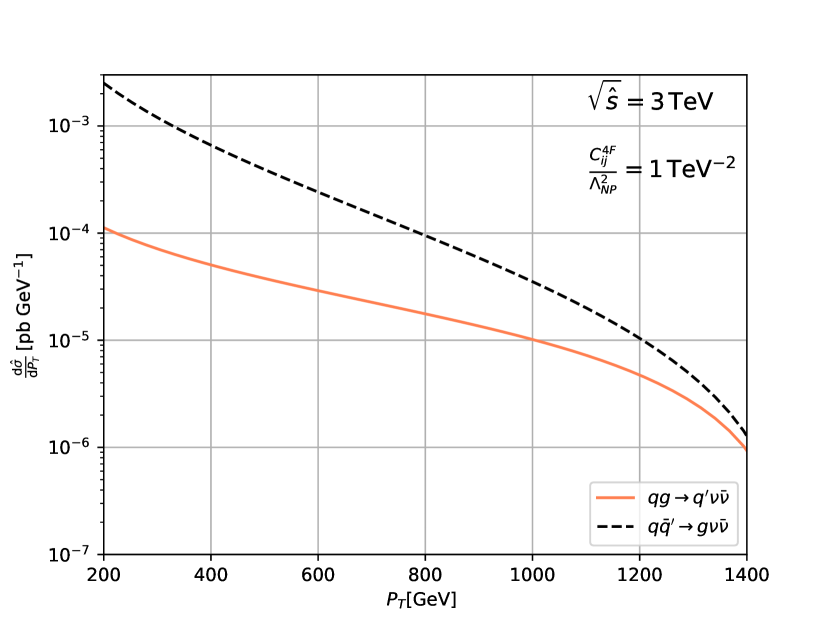
(a)

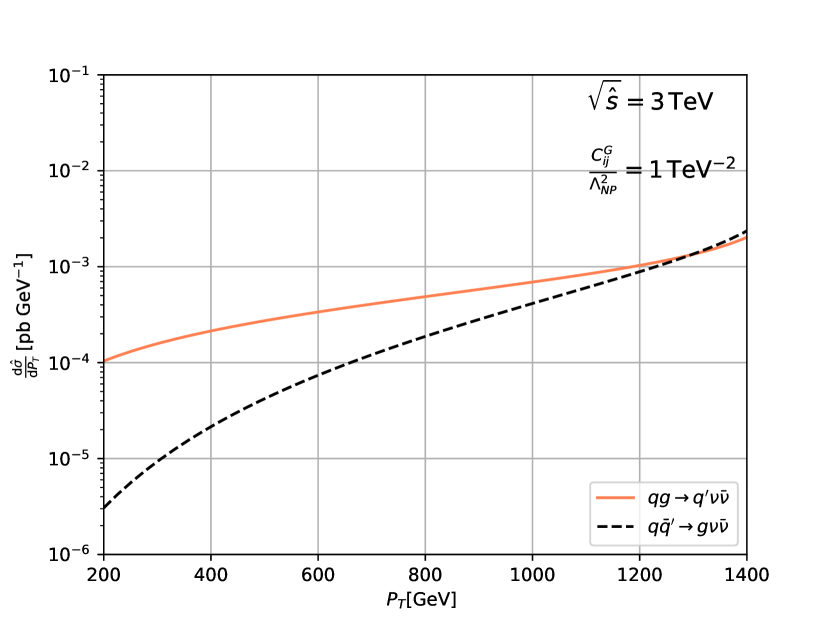
(b)

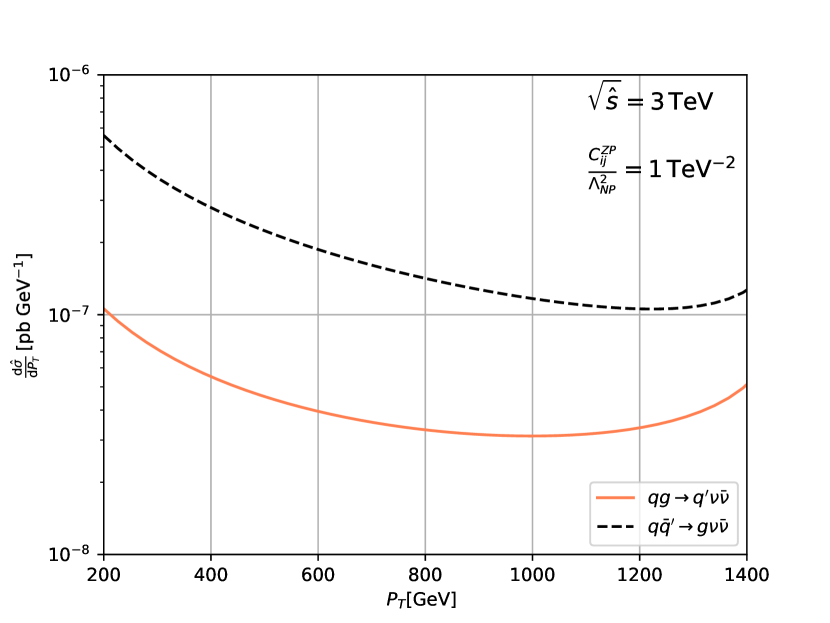
(c)

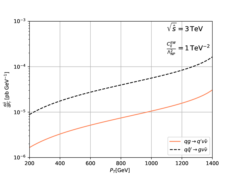
(d)

Figure 7: Comparison of partonic cross sections of $qg$ (orange, solid) and $q\bar{q}$ (black, dashed) contributions for the effective WCs $C^{4F}_{ij}$ (a), $C^{G}_{ij}$ (b), $C^{ZP}_{ij}$ (c) and $C^{EW}_{ij}$ (d) as defined in Secs. II.2,II.3 and II.4. Note that in (b) the difference between up- and down-sector is not shown, since the difference is below $1\%$.

B.3.1 SM prediction

The $P_{T}$-spectra are then given in the NWA

$$\frac{\mathrm{d}\hat{\sigma}(q_{i}\bar{q}_{j}\rightarrow\nu\bar{\nu}g)}{\mathrm{d}P_{T}} =\frac{4\alpha_{s}\left({\epsilon_{L}^{i,j}}^{2}+{\epsilon_{R}^{i,j}}^{2}\right)\text{Br}\left(Z\rightarrow\nu\bar{\nu}\right)}{9}\frac{M_{Z}^{4}+\hat{s}(\hat{s}-2P_{T}^{2})}{P_{T}\hat{s}^{2}\sqrt{(\hat{s}-M_{Z}^{2})^{2}-4P_{T}^{2}\hat{s}}}$$ (86)

$$\frac{\mathrm{d}\hat{\sigma}(q_{i}g\rightarrow\nu\bar{\nu}q_{j})}{\mathrm{d}P_{T}} =-\frac{\alpha_{s}\left({\epsilon_{L}^{i,j}}^{2}+{\epsilon_{R}^{i,j}}^{2}\right)\text{Br}\left(Z\rightarrow\nu\bar{\nu}\right)}{12}$$ (87)

$$\times\frac{2M_{Z}^{6}-4M_{Z}^{2}\hat{s}+3M_{Z}^{2}\hat{s}(\hat{s}-P_{T}^{2})-\hat{s}^{2}(P_{T}^{2}+\hat{s})}{P_{T}\hat{s}^{3}\sqrt{(\hat{s}-M_{Z}^{2})^{2}-4P_{T}^{2}\hat{s}}}$$

In the high energy limit these approach

$$\frac{\mathrm{d}\hat{\sigma}(q_{i}\bar{q}_{j}\rightarrow\nu\bar{\nu}g)}{\mathrm{d}P_{T}} \approx\frac{4\sqrt{2}\alpha_{s}\text{Br}(Z\rightarrow\nu\bar{\nu})\left({\epsilon_{L}^{i,j}}^{2}+{\epsilon_{R}^{i,j}}^{2}\right)}{9}\frac{1}{\hat{s}^{3/2}}\frac{2-x^{2}}{x\sqrt{1-x^{2}}}$$ (89)

$$\frac{\mathrm{d}\hat{\sigma}(q_{i}g\rightarrow\nu\bar{\nu}q_{j})}{\mathrm{d}P_{T}} \approx\frac{\alpha_{s}\text{Br}(Z\rightarrow\nu\bar{\nu})\left({\epsilon_{L}^{i,j}}^{2}+{\epsilon_{R}^{i,j}}^{2}\right)}{12\sqrt{2}}\frac{1}{\hat{s}^{3/2}}\frac{x^{2}+4}{x\sqrt{1-x^{2}}}$$ (90)

B.3.2 Four-fermion operators

The results for 4F operators can be integrated analytically and the $P_{T}$-spectrum can be given in terms of the scaling variable $x=2P_{T}/\sqrt{\hat{s}}$:

$$\frac{\mathrm{d}\hat{\sigma}(q_{i}\bar{q}_{j}\rightarrow\nu\bar{\nu}g)}{\mathrm{d}P_{T}} =\frac{\alpha_{s}{C^{4F}_{ij}}^{2}}{162\pi^{2}\Lambda^{4}}\sqrt{\hat{s}}\;\frac{6(x^{2}+2)\cosh^{-1}\left(x^{-1}\right)-(x^{2}+17)\sqrt{1-x^{2}}}{x}$$ (91)

$$\frac{\mathrm{d}\hat{\sigma}(q_{i}g\rightarrow\nu\bar{\nu}q_{j})}{\mathrm{d}P_{T}} =\frac{\alpha_{s}{C^{4F}_{ij}}^{2}}{3456\pi^{2}\Lambda^{4}}\sqrt{\hat{s}}\;\frac{3x^{2}(3x^{2}+4)\cosh^{-1}\left(x^{-1}\right)-(13x^{2}+8)\sqrt{1-x^{2}}}{x}$$ (92)

For $P_{T}\sim\sqrt{\hat{s}}/2$ ($x\rightarrow 1$) these read

$$\frac{\mathrm{d}\hat{\sigma}(q_{i}\bar{q}_{j}\rightarrow\nu\bar{\nu}g)}{\mathrm{d}P_{T}} \approx\frac{\sqrt{2}\alpha_{s}{C^{4F}_{ij}}^{2}}{81\pi^{2}}\frac{1}{\Lambda^{4}}\sqrt{\hat{s}}(1-x)^{3/2}$$ (93)

$$\frac{\mathrm{d}\hat{\sigma}(q_{i}g\rightarrow\nu\bar{\nu}q_{j})}{\mathrm{d}P_{T}} \approx\frac{5\alpha_{s}{C^{4F}_{ij}}^{2}}{432\sqrt{2}\pi^{2}}\frac{1}{\Lambda^{4}}\sqrt{\hat{s}}(1-x)^{3/2}\;$$ (94)

B.3.3 Z-penguin operators

The $P_{T}$-spectra are then given in the NWA

$$\frac{\mathrm{d}\hat{\sigma}(q_{i}\bar{q}_{j}\rightarrow\nu\bar{\nu}g)}{\mathrm{d}P_{T}} =\frac{4\alpha_{s}M_{Z}^{2}v^{2}{C^{ZP}_{i,j}}^{2}\text{Br}\left(Z\rightarrow\nu\bar{\nu}\right)}{9\Lambda^{4}}\frac{M_{Z}^{4}+\hat{s}(\hat{s}-2P_{T}^{2})}{P_{T}\hat{s}^{2}\sqrt{(\hat{s}-M_{Z}^{2})^{2}-4P_{T}^{2}\hat{s}}}$$ (95)

$$\frac{\mathrm{d}\hat{\sigma}(q_{i}g\rightarrow\nu\bar{\nu}q_{j})}{\mathrm{d}P_{T}} =-\frac{\alpha_{s}M_{Z}^{2}{C^{ZP}_{i,j}}^{2}\text{Br}\left(Z\rightarrow\nu\bar{\nu}\right)}{12\sqrt{2}G_{F}\Lambda^{4}}$$ (96)

$$\times\frac{2M_{Z}^{6}-4M_{Z}^{2}\hat{s}+3M_{Z}^{2}\hat{s}(\hat{s}-P_{T}^{2})-\hat{s}^{2}(P_{T}^{2}+\hat{s})}{P_{T}\hat{s}^{3}\sqrt{(\hat{s}-M_{Z}^{2})^{2}-4P_{T}^{2}\hat{s}}}$$

In the high energy limit these approach

$$\frac{\mathrm{d}\hat{\sigma}(q_{i}\bar{q}_{j}\rightarrow\nu\bar{\nu}g)}{\mathrm{d}P_{T}} \approx\frac{4\alpha_{s}{C^{ZP}_{i,j}}^{2}\text{Br}\left(Z\rightarrow\nu\bar{\nu}\right)}{9}\frac{M_{Z}^{2}v^{2}}{\Lambda^{4}}\frac{1}{\hat{s}^{3/2}}\frac{2-x^{2}}{x\sqrt{1-x^{2}}}$$ (97)

$$\frac{\mathrm{d}\hat{\sigma}(q_{i}g\rightarrow\nu\bar{\nu}q_{j})}{\mathrm{d}P_{T}} \approx\frac{\alpha_{s}{C^{ZP}_{i,j}}^{2}\text{Br}\left(Z\rightarrow\nu\bar{\nu}\right)}{24}\frac{M_{Z}^{2}v^{2}}{\Lambda^{4}}\frac{1}{\hat{s}^{3/2}}\frac{4+x^{2}}{x\sqrt{1-x^{2}}}$$ (98)

Note that $C^{ZP}_{i,j}$ here is the definition from equation (10), since at parton level the flavors do not mix and therefore the definition holds for all $i,j$.

B.3.4 EW dipole operators

The $P_{T}$-spectra are then given in the NWA

$$\frac{\mathrm{d}\hat{\sigma}(q_{i}\bar{q}_{j}\rightarrow\nu\bar{\nu}g)}{\mathrm{d}P_{T}} =\frac{4v^{2}\alpha_{s}{C^{EW}_{i,j}}^{2}\text{Br}\left(Z\rightarrow\nu\bar{\nu}\right)}{9\Lambda^{4}}\frac{M_{Z}^{2}\hat{s}(\hat{s}-4P_{T}^{2})+4P_{T}^{2}\hat{s}^{2}+M_{Z}^{6}}{P_{T}\hat{s}^{2}\sqrt{(\hat{s}-M_{Z}^{2})^{2}-4P_{T}^{2}\hat{s}}}$$ (99)

$$\frac{\mathrm{d}\hat{\sigma}(q_{i}g\rightarrow\nu\bar{\nu}q_{j})}{\mathrm{d}P_{T}} =\frac{-v^{2}\alpha_{s}{C^{EW}_{i,j}}^{2}\text{Br}\left(Z\rightarrow\nu\bar{\nu}\right)}{12\Lambda^{4}}$$ (100)

$$\times\frac{\left(3M_{Z}^{4}\hat{s}(P_{T}^{2}-\hat{s})+M_{Z}^{2}\hat{s}^{2}(P_{T}^{2}+\hat{s})+4P_{T}^{2}\hat{s}^{3}-2M_{Z}^{8}+4M_{Z}^{6}\hat{s}\right)}{P_{T}\hat{s}^{3}\sqrt{(\hat{s}-M_{Z}^{2})^{2}-4P_{T}^{2}\hat{s}}}$$

In the high energy limit these approach

$$\frac{\mathrm{d}\hat{\sigma}(q_{i}\bar{q}_{j}\rightarrow\nu\bar{\nu}g)}{\mathrm{d}P_{T}} \approx\frac{4\alpha_{s}{C^{EW}_{i,j}}^{2}\text{Br}\left(Z\rightarrow\nu\bar{\nu}\right)}{9}\frac{v^{2}}{\Lambda^{4}}\frac{1}{\sqrt{\hat{s}}}\frac{x}{\sqrt{1-x^{2}}}$$ (101)

$$\frac{\mathrm{d}\hat{\sigma}(q_{i}g\rightarrow\nu\bar{\nu}q_{j})}{\mathrm{d}P_{T}} \approx\frac{\alpha_{s}{C^{EW}_{i,j}}^{2}\text{Br}\left(Z\rightarrow\nu\bar{\nu}\right)}{6}\frac{v^{2}}{\Lambda^{4}}\frac{1}{\sqrt{\hat{s}}}\frac{x}{\sqrt{1-x^{2}}}$$ (102)

B.3.5 G dipole operators

The $P_{T}$-spectra are then given in the NWA, for the up- and down-sector,

$$\frac{\mathrm{d}\hat{\sigma}(q_{i}\bar{q}_{j}\rightarrow\nu\bar{\nu}g)}{\mathrm{d}P_{T}} =\frac{{C^{G}_{i,j}}^{2}\text{Br}\left(Z\rightarrow\nu\bar{\nu}\right)v^{2}}{9\pi M_{Z}^{2}\Lambda^{4}}\frac{P_{T}\left(2M_{Z}^{2}\left({\epsilon_{L}^{i,j}}^{2}+{\epsilon_{R}^{i,j}}^{2}\right)+\left(\epsilon_{L}^{i,j}-{\epsilon_{R}^{i,j}}\right)^{2}P_{T}^{2}\right)}{\sqrt{(M_{Z}^{2}-\hat{s})^{2}-4P_{T}^{2}\hat{s}}}$$ (103)

$$\frac{\mathrm{d}\hat{\sigma}(q_{i}g\rightarrow\nu\bar{\nu}q_{j})}{\mathrm{d}P_{T}} =\frac{{C^{G}_{i,j}}^{2}\text{Br}\left(Z\rightarrow\nu\bar{\nu}\right)v^{2}}{48\pi M_{Z}^{2}\Lambda^{4}}$$ (104)

$$\times\left(\hat{s}-M_{Z}^{2}\right)\frac{P_{T}\left(2M_{Z}^{2}\left({\epsilon_{L}^{i,j}}^{2}+{\epsilon_{R}^{i,j}}^{2}\right)+\left(\epsilon_{L}^{i,j}-{\epsilon_{R}^{i,j}}\right)^{2}\hat{s}^{2}\right)}{\hat{s}\sqrt{(M_{Z}^{2}-\hat{s})^{2}-4P_{T}^{2}\hat{s}}}$$

In the high energy limit the different sectors converge to the same result

$$\frac{\mathrm{d}\hat{\sigma}(q_{i}\bar{q}_{j}\rightarrow\nu\bar{\nu}g)}{\mathrm{d}P_{T}} \approx\frac{{C^{G}_{i,j}}^{2}\text{Br}\left(Z\rightarrow\nu\bar{\nu}\right)\left(\epsilon_{L}^{i,j}-{\epsilon_{R}^{i,j}}\right)^{2}v^{2}}{72\pi M_{Z}^{2}}\frac{1}{\Lambda^{4}}\sqrt{\hat{s}}\frac{x^{3}}{\sqrt{1-x^{2}}}$$ (105)

$$\frac{\mathrm{d}\hat{\sigma}(q_{i}g\rightarrow\nu\bar{\nu}q_{j})}{\mathrm{d}P_{T}} \approx\frac{{C^{G}_{i,j}}^{2}\text{Br}\left(Z\rightarrow\nu\bar{\nu}\right)\left(\epsilon_{L}^{i,j}-{\epsilon_{R}^{i,j}}\right)^{2}v^{2}}{96\pi M_{Z}^{2}}\frac{1}{\Lambda^{4}}\sqrt{\hat{s}}\frac{x}{\sqrt{1-x^{2}}}$$ (106)

References

- Buchmuller and Wyler (1986) W. Buchmuller and D. Wyler, Nucl. Phys. B 268, 621 (1986).
- Grzadkowski et al. (2010) B. Grzadkowski, M. Iskrzynski, M. Misiak, and J. Rosiek, JHEP 10, 085 (2010), eprint 1008.4884.
- Drell and Yan (1970) S. D. Drell and T.-M. Yan, Phys. Rev. Lett. 25, 316 (1970), [Erratum: Phys.Rev.Lett. 25, 902 (1970)].
- Aoude et al. (2020) R. Aoude, T. Hurth, S. Renner, and W. Shepherd, JHEP 12, 113 (2020), eprint 2003.05432.
- Bruggisser et al. (2021) S. Bruggisser, R. Schäfer, D. van Dyk, and S. Westhoff, JHEP 05, 257 (2021), eprint 2101.07273.
- Greljo et al. (2023) A. Greljo, J. Salko, A. Smolkovič, and P. Stangl, JHEP 05, 087 (2023), eprint 2212.10497.
- Grunwald et al. (2023) C. Grunwald, G. Hiller, K. Kröninger, and L. Nollen, JHEP 11, 110 (2023), eprint 2304.12837.
- Farina et al. (2017) M. Farina, G. Panico, D. Pappadopulo, J. T. Ruderman, R. Torre, and A. Wulzer, Phys. Lett. B 772, 210 (2017), eprint 1609.08157.
- Greljo and Marzocca (2017) A. Greljo and D. Marzocca, Eur. Phys. J. C 77, 548 (2017), eprint 1704.09015.
- Fuentes-Martin et al. (2020) J. Fuentes-Martin, A. Greljo, J. Martin Camalich, and J. D. Ruiz-Alvarez, JHEP 11, 080 (2020), eprint 2003.12421.
- Aad et al. (2021a) G. Aad et al. (ATLAS), Phys. Rev. D 103, 112006 (2021a), eprint 2102.10874.
- Tumasyan et al. (2021) A. Tumasyan et al. (CMS), JHEP 11, 153 (2021), eprint 2107.13021.
- Cepeda et al. (2019) M. Cepeda et al., CERN Yellow Rep. Monogr. 7, 221 (2019), eprint 1902.00134.
- Bause et al. (2022) R. Bause, H. Gisbert, M. Golz, and G. Hiller, Eur. Phys. J. C 82, 164 (2022), eprint 2007.05001.
- Aebischer et al. (2016) J. Aebischer, A. Crivellin, M. Fael, and C. Greub, JHEP 05, 037 (2016), eprint 1512.02830.
- Bißmann et al. (2021) S. Bißmann, C. Grunwald, G. Hiller, and K. Kröninger, JHEP 06, 010 (2021), eprint 2012.10456.
- Butterworth et al. (2016) J. Butterworth et al., J. Phys. G 43, 023001 (2016), eprint 1510.03865.
- Harland-Lang et al. (2015) L. A. Harland-Lang, A. D. Martin, P. Motylinski, and R. S. Thorne, Eur. Phys. J. C 75, 204 (2015), eprint 1412.3989.
- Ball et al. (2015) R. D. Ball et al., JHEP 04, 040 (2015), eprint 1410.8849.
- Dulat et al. (2016) S. Dulat, T.-J. Hou, J. Gao, M. Guzzi, J. Huston, P. Nadolsky, J. Pumplin, C. Schmidt, D. Stump, and C. P. Yuan, Phys. Rev. D 93, 033006 (2016), eprint 1506.07443.
- Angelescu et al. (2020) A. Angelescu, D. A. Faroughy, and O. Sumensari, Eur. Phys. J. C 80, 641 (2020), eprint 2002.05684.
- Lam and Tung (1978) C. S. Lam and W.-K. Tung, Phys. Rev. D 18, 2447 (1978).
- Schael et al. (2006) S. Schael et al. (ALEPH, DELPHI, L3, OPAL, SLD, LEP Electroweak Working Group, SLD Electroweak Group, SLD Heavy Flavour Group), Phys. Rept. 427, 257 (2006), eprint hep-ex/0509008.
- Frederix et al. (2018) R. Frederix, S. Frixione, V. Hirschi, D. Pagani, H. S. Shao, and M. Zaro, JHEP 07, 185 (2018), [Erratum: JHEP 11, 085 (2021)], eprint 1804.10017.
- Brivio (2021) I. Brivio, JHEP 04, 073 (2021), eprint 2012.11343.
- Bierlich et al. (2022) C. Bierlich et al. (2022), eprint 2203.11601.
- de Favereau et al. (2014) J. de Favereau, C. Delaere, P. Demin, A. Giammanco, V. Lemaître, A. Mertens, and M. Selvaggi (DELPHES 3), JHEP 02, 057 (2014), eprint 1307.6346.
- Cacciari et al. (2012) M. Cacciari, G. P. Salam, and G. Soyez, Eur. Phys. J. C 72, 1896 (2012), eprint 1111.6097.
- Read (2002) A. L. Read, J. Phys. G 28, 2693 (2002).
- (30) L. Heinrich, M. Feickert, and G. Stark, pyhf: v0.7.0rc1, https://github.com/scikit-hep/pyhf/releases/tag/v0.7.0rc1, URL https://doi.org/10.5281/zenodo.1169739.
- Workman et al. (2022) R. L. Workman et al. (Particle Data Group), PTEP 2022, 083C01 (2022).
- Haisch and Koole (2021) U. Haisch and G. Koole, JHEP 09, 133 (2021), eprint 2106.01289.
- Fajfer et al. (2023) S. Fajfer, J. F. Kamenik, N. Košnik, A. Smolkovič, and M. Tammaro (2023), eprint 2306.16471.
- Alonso et al. (2014) R. Alonso, E. E. Jenkins, A. V. Manohar, and M. Trott, JHEP 04, 159 (2014), eprint 1312.2014.
- Aebischer et al. (2018) J. Aebischer, J. Kumar, and D. M. Straub, Eur. Phys. J. C 78, 1026 (2018), eprint 1804.05033.
- de Boer and Hiller (2017) S. de Boer and G. Hiller, JHEP 08, 091 (2017), eprint 1701.06392.
- Adolph et al. (2021) N. Adolph, J. Brod, and G. Hiller, Eur. Phys. J. C 81, 45 (2021), eprint 2009.14212.
- Golz et al. (2021) M. Golz, G. Hiller, and T. Magorsch, JHEP 09, 208 (2021), eprint 2107.13010.
- Lyon and Zwicky (2022) J. Lyon and R. Zwicky, Phys. Rev. D 106, 053001 (2022), eprint 1210.6546.
- Giudice et al. (2012) G. F. Giudice, G. Isidori, and P. Paradisi, JHEP 04, 060 (2012), eprint 1201.6204.
- Bause et al. (2023) R. Bause, H. Gisbert, M. Golz, and G. Hiller, Eur. Phys. J. C 83, 419 (2023), eprint 2209.04457.
- Mahmoudi et al. (2023) F. Mahmoudi, T. Hurth, D. Martínez Santos, and S. Neshatpour, EPJ Web Conf. 289, 01002 (2023).
- Aad et al. (2021b) G. Aad et al. (ATLAS), JHEP 02, 226 (2021b), eprint 2011.05259.
- Bause et al. (2021a) R. Bause, H. Gisbert, M. Golz, and G. Hiller, Phys. Rev. D 103, 015033 (2021a), eprint 2010.02225.
- Ablikim et al. (2022) M. Ablikim et al. (BESIII), Phys. Rev. D 105, L071102 (2022), eprint 2112.14236.
- Bause et al. (2021b) R. Bause, H. Gisbert, M. Golz, and G. Hiller, JHEP 12, 061 (2021b), eprint 2109.01675.
- Dedes et al. (2017) A. Dedes, W. Materkowska, M. Paraskevas, J. Rosiek, and K. Suxho, JHEP 06, 143 (2017), eprint 1704.03888.