AXES-2MRS: A new all-sky catalogue of extended X-ray galaxy groups

Abstract

Context. Understanding the baryonic physics on the galaxy group level is a prerequisite for cosmological studies of large-scale structure. One poorly understood aspect of galaxy groups is related to the properties of their hot intragroup medium. The well-studied X-ray groups have strong cool cores by which they were selected, so expanding the selection of groups is currently an important venue.

Aims. We present a new all-sky catalogue of X-ray detected groups (AXES-2MRS), based on the identification of large X-ray sources found in the ROSAT All-Sky Survey (RASS) with the Two Micron Redshift Survey (2MRS) Bayesian Group Catalogue. We study the basic properties of these galaxy groups to gain insights into the effect of different group selections on the properties.

Methods. In addition to X-ray luminosity coming from shallow survey data of RASS, we have obtained detailed X-ray properties of the groups by matching the AXES-2MRS catalogue to archival X-ray observations by XMM-Newton and complemented this by adding the published XMM-Newton results on galaxy clusters in our catalogue. We analyse temperature and density to the lowest overdensity accessible by the data, obtaining hydrostatic mass estimates and comparing them to the velocity dispersions of the groups. We explore the relationship between X-ray and optical properties of AXES-2MRS groups through the $\sigma_{\mathrm{v}}-L_{\mathrm{X}}$, $\sigma_{\mathrm{v}}-kT$, $kT-L_{\mathrm{X}}$, $\sigma_{\mathrm{v}}-M$, and $c_{200}-L_{\rm X}$ scaling relations.

Results. We find a large spread in the central mass to virial mass ratios for galaxy groups in the XMM-Newton subsample. This can either indicate large non-thermal pressure of galaxy groups affecting our X-ray mass measurements, or the effect of a diversity of halo concentrations on X-ray properties of galaxy groups. Previous catalogues, based on detecting the peak of the X-ray emission preferentially sample the high-concentration groups, while our new catalogue includes many low-concentration groups.

1 Introduction

The hot intergalactic medium of galaxy groups plays an important role in galaxy evolution and reflects the energetics of galactic outflows and metal production. Several studies have suggested a direct link between the baryonic content of galaxy groups and the shape of matter power spectrum on spatial scales below 10 Mpc (Debackere et al., 2020). Deep X-ray surveys enabled significant advances in understanding galaxy groups, which discovered a large population of X-ray emitting groups down to the mass below $10^{13}M_{\odot}$ and reaching redshifts above 2 on high-mass groups (Gozaliasl et al., 2019). However, the low-redshift ($z<0.1$) population of galaxy groups still lacks a full understanding. In contrast, this population is a main source of our knowledge on the detailed properties of galaxy groups. Previous catalogues of X-ray-selected local groups and clusters of galaxies were primarily based on identifying sources encompassing the emitting zone of $2^{\prime}$. This has been shown to account for only a fraction of galaxy groups consisting of relaxed groups with luminous central objects (Mulchaey, 2000). A large population of sources is omitted from these catalogues (Xu et al., 2018), which is confirmed by the dedicated consideration of galaxy group emission by Käfer et al. (2019). In this paper we will continue the investigation of such sources, considering the spatially resolved X-ray emission down to the lowest signal-to-noise ratio (SNR) of the ROSAT All-Sky Survey (RASS) and detected on virial spatial scales.

This paper is organized as follows: in Section 2, we present the construction and basic properties of the new X-ray source catalogue, describe the 2MRS optical group catalogue used for the identification, and introduce a representative subsample observed by XMM-Newton. The analysis of X-ray and optical properties of X-ray detected groups in our catalogue is provided in Section 3. In Section 4, we present the scaling relations including a comparison with the literature. We summarize our results in Section 5. In this study, we adopt a flat $\Lambda$CDM cosmology with parameters $H_{0}$ = 70 km s^-1 Mpc^-1, $\Omega_{\rm m}$ = 0.3, and $\Omega_{\Lambda}=1-\Omega_{\rm m}$. Unless otherwise stated, errors represent standard $1\sigma$ uncertainties (drawn at the 68$\%$ confidence level). For radii, masses, and concentrations, the suffixes 200, 500, and 10000 correspond to the mean densities relative to the critical density of the Universe at the redshift of the group.

2 Data

Figure 1: Cumulative distribution for the X-ray flux in the 0.5–2.0 keV band per sky area ($\log N-\log S$) for AXES X-ray sources (black), and AXES-2MRS groups (blue). AXES X-ray sources in the extragalactic region (nH $<5\times 10^{20}$ cm^-2) are shown in purple, while extragalactic AXES-2MRS groups are shown in red. The flux of the AXES-2MRS sources has been extrapolated to $R_{500}$, while for AXES we show the measured flux.

2.1 AXES: a new catalogue of X-ray sources from ROSAT All Sky Survey

The ROSAT all-sky survey (RASS) has been an enormous legacy for X-ray astronomy (see Truemper, 1993, for a review). Of particular importance are the all-sky catalogues of sources (Voges et al., 1999), which formed the base of X-ray studies in the last three decades. Exploration of the RASS data down to its faint limits has recently become an active field (e.g., Finoguenov et al., 2020). In the present paper, we report a new study of RASS data. We have produced a new catalogue of RASS sources, All-sky X-ray Extended Sources (AXES), found using 0.5–2.0 keV band images. For the source detection and determination of the flux extraction regions, we employ the wavelet scales of 12 or 24 arcmin after removing the emission detected on scales of 6 arcmin and below. This is a multiscale detection, unaffected by the emission on scales smaller than the scale of interest. We construct the experiment to scale with the baryonic content of galaxy groups near $R_{500}$, which is different from the point of finding spatially resolved X-ray sources on scales of the point spread function, which forms a base of the Xu et al. (2018) catalogue. By reducing the dependence of the detection on the shape of X-ray emission in the centre, the modelling of the source detection becomes feasible through the use of currently available hydrodynamical simulations, which reproduce group outskirts, but not the group cores. In Fig. 1, we show the normalized cumulative number count of AXES sources and AXES-2MRS groups (see Section 2.2) as a function of the flux in the 0.5–2.0 keV band ($\log N-\log S$). We do not attempt to restore the original $\log N-\log S$, but rather to look for indications of the catalogue completeness. On the adopted spatial scales the detection is background limited and completeness as a function of flux indicates a completeness limit of $2\times 10^{-12}$ ergs s^-1 cm^-2 (see Fig. 1), which is characteristic of the extragalactic areas. The 2MRS survey (see Section 2.2) stops where X-ray sensitivity drops by a factor of two due to foreground absorption. When comparing the $\log N-\log S$ distribution inside and outside the zone of avoidance, we see an excess of the bright sources in the zone of avoidance, which we attribute to additional sources coming from the galactic plane. We also note that at fluxes fainter than $10^{-11}$ erg s^-1 cm² the two curves converge, which indicates a predominance of extragalactic sources at those fluxes even in the galactic plane. AXES contains over six thousand unique X-ray sources, with a large concentration of sources towards the galactic centre, with many of them identified with supernova remnants. Therefore, to report on a new galaxy group, external identification of sources is required.

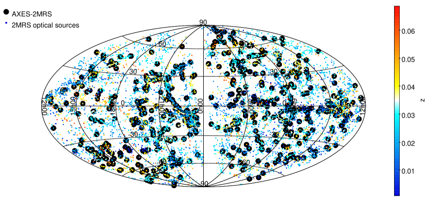
Figure 2: Distribution of AXES-2MRS X-ray sources and full 2MRS optical sources represented with supergalactic coordinates on the sky. The small points are 2MRS optical groups bar coloured according to their (CMB rest frame corrected) redshift, while larger black circles denote the full AXES-2MRS X-ray catalogue of 558 groups.

2.2 Optical Group Catalogue

The choice of the angular scales for our X-ray detection is designed to cover the virial radius of groups at $z<0.1$. To identify the sources we find with AXES in this work, we consider a group catalogue from the 2MASS spectroscopic survey (Tempel et al., 2018, 2MRS), selecting the groups that contain at least three spectroscopic members. The advantage of this catalogue is that it is all-sky and extends into the galactic disk, allowing us to improve on the studies of the local dynamics. In assigning the X-ray sources to the optical group, we compute the radius of 200 kpc using the redshift of the group and use it to find an X-ray counterpart within this radius. Using the redshift of the group and the H i absorption-corrected flux of the X-ray source, we then compute the source rest-frame X-ray luminosity in the 0.1–2.4 keV band, with K-corrections obtained iteratively using the $L-T$ relation. Our choice of using 2MRS groups down to 3 spectroscopic members is an attempt to improve the completeness of the 2MRS towards $10^{13}M_{\odot}$ groups expected to emit X-rays while avoiding the inclusion of a large population of low-mass groups (with masses extending down to $10^{12}M_{\odot}$), present in the two-member catalogue (for a discussion of tracing group mass with a few members see e.g. Knobel et al., 2009). Our choice of a minimum of 3 members compares well with the results of REFLEX spectroscopic identification (Böhringer et al., 2004), which made the largest contribution to the exhaustive X-ray cluster catalogue MCXC (Piffaretti et al., 2011). Given the small number of sources and the high fraction of matches, AXES-2MRS has a high level of purity of 97%. Given the importance of the low-z systems to the studies of the local dynamics, we do not cut the catalogue to the extragalactic areas, which is uniquely possible given our choice of source identification using the 2MRS catalogue. In Fig.2 we show the sky distribution of the groups in AXES-2MRS using a supergalactic coordinate system. We use the symbol’s colour to illustrate the group’s redshift. X-ray sources identified with the groups are marked with large black-filled circles. Most groups in the 2MRS catalogue have no mass estimates, given they have just a few members. Our catalogue improves this situation by providing an X-ray luminosity estimate, which is a mass proxy, and marks the massive parts of the local cosmic web. In the application of X-ray studies to the Galactic areas, it is important to acknowledge technological differences in X-ray detectors. ROSAT PSPC detector, used in RASS, is based on the photon interaction with gas, which is not sensitive to stellar light, and is a serious problem for X-ray CCDs. On XMM-Newton, this problem is addressed by selecting an appropriate filter for the observation. However, this is not done for eROSITA, resulting in an additional source of contamination, absent in RASS. Thus, the AXES catalogue provides a reliable list of sources, against which to compare CCD detections on comparable spatial and flux scales.

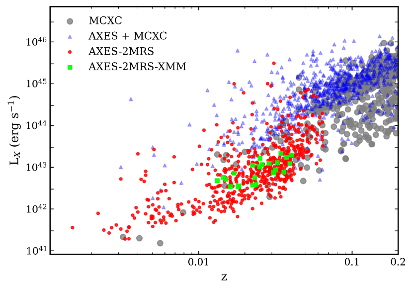
Figure 3: Full AXES-2MRS catalogue (558 groups, red circles) compared to overlapping systems between MCXC and AXES-2MRS (blue triangles), and unique MCXC systems (grey circles) in the $L_{\rm X}-z$ plane. The XMM-Newton-observed subset with at least eight members selected from AXES-2MRS is shown with neon green squares.

To demonstrate the state of our new catalogue relative to the literature, we compare it with the MCXC in the $L_{\rm X}-z$ plane in Fig. 3. The MCXC consists of 1743 unique cluster detections representing a compilation of different catalogues based on RASS data, and ROSAT pointed data. Using MCXC mass estimates we find 905 AXES sources to be located inside $R_{200}$ of 838 unique clusters. In Fig.3 we plot the full MCXC catalogue, zooming on the low-redshift ($z<0.2$) subspace, its overlap with AXES sources, and present the AXES-2MRS catalogue. MCXC, being a literature compilation catalogue, reveals clear signatures of different completeness below and above $10^{44}$ ergs s^-1. Nevertheless, for our purpose of illustrating the limitations imposed by using 2MRS as follow-up data, it is sufficient. The AXES-2MRS sources are limited to $z<0.08$ with incompleteness signatures appearing at $z>0.04$, which match the expectations on the completeness of the 2MRS catalogue. At $z>0.1$, the extent of X-ray emission reaches AXES detection scales only for the most massive clusters, so the selection effects become noticeable close to a redshift of 0.2. At $z<0.04$ AXES-2MRS luminosities are located well on the extrapolation of the MCXC trends towards lower redshift, while MCXC itself does not have many systems in the same redshift range. We also cross-matched AXES-2MRS with the newly released X-ray-selected extended galaxy cluster catalogue (RXGCC, Xu et al. 2022), which is based on RASS and contains 944 systems. Within a 5^′ radius (positional uncertainty of large X-ray sources at lowest detection significance), we identified 162 overlapping systems, out of a total number of 558 AXES-2MRS groups. To further illustrate the role of AXES-2MRS in enhancing the completeness of X-ray group catalogues, we compared our catalogue to the extensive eROSITA-based catalogue of galaxy clusters and groups (Bulbul et al., 2024, eRASS1). With over 12,200 systems, eRASS1 covers a total of 13,116 deg² in the western Galactic hemisphere of the sky and has a redshift range of $0.003<z<1.32$. Despite the majority (68$\%$) of eRASS1 systems being new identifications with no counterparts in the literature, we could match only 73 overlapping groups with AXES-2MRS within a 5^′ radius and a redshift tolerance of 0.01. The published eRASS1 catalogues reach much fainter fluxes, but the source detection is limited to $3^{\prime}$, which is not optimal for low-redshift groups (Käfer et al., 2019). In addition, the red sequence identification, employed in the identification of eRASS1 sources, is incomplete for groups (Rykoff et al., 2014).

The all-sky distribution of the identified AXES-2MRS X-ray groups overlaid with the galaxy compilation used to create the 2MRS optical catalogue is shown in Fig. 5. The figure is split about the equator into two declination regions: the top panel shows the northern [$0^{\circ}<\text{Dec}\leq 90^{\circ}$] range with 316 AXES-2MRS groups and 21484 galaxies. While the bottom panel shows the southern [$-90^{\circ}\leq\text{Dec}\leq 0^{\circ}$] range with 242 AXES-2MRS groups and 20727 galaxies. The maps show the location of the largest local structures in the Universe, on which 2MRS-AXES sources mark the most massive virialized systems. In addition, we mark the locations of the local underdensity regions (voids) taken from Plionis & Basilakos (2002); Tully et al. (2019). The former work detected voids in the PCSz redshift survey (Saunders et al., 2000), while the latter modelled the morphology of the local voids using peculiar velocities.

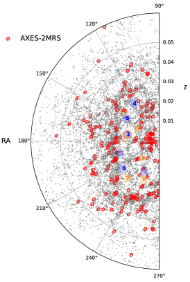
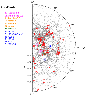
(a) $0^{\circ}<\text{Dec}\leq 90^{\circ}$

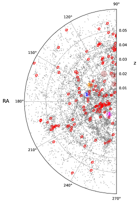
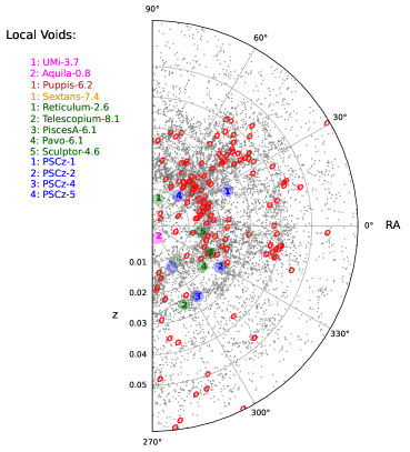
(b) $-90^{\circ}\leq\text{Dec}\leq 0^{\circ}$

Figure 5: Projection of the 3-dimensional distribution of local cosmic structure onto the RA-redshift plane, illustrating the correspondence of the AXES-2MRS groups (red ellipses) to large-scale structure traced by the 2MRS galaxies (grey dots), with the location of the largest local voids marked. The coloured regions denote void centres, but their sizes do not reflect void dimensions. Pink regions/labels are density minima in the Local Void, orange is the Hercules Void, while green and brown represent the Sculptor and Eridanus Voids, respectively. Blue colour denotes the PSCz-IRAS survey data (Plionis & Basilakos, 2002), while the other voids are based on Tully et al. (2019). (a) Northern hemisphere (positive Dec values). (b) Southern hemisphere (negative Dec values).

2.3 XMM-Newton Data

For a subset of AXES-2MRS groups, we obtained a much more detailed picture of the group emission using XMM-Newton observations. We have searched the archival XMM-Newton data on the sample, limiting the study to the groups having at least 8 spectroscopic members, retained after cleaning the membership using Clean (Mamon et al., 2013). Our XMM-Newton data reduction pipeline is described in Finoguenov et al. (2007). We have used the XMMSAS version 21.0.0. In the imaging analysis, we used the 0.5–2 keV band, removing instrument lines, as described in Finoguenov et al. (2007). Point source detection and removal have been performed following Finoguenov et al. (2010). We perform the wavelet decomposition (Vikhlinin et al., 1998, ) of the extended emission on scales from half an arcminute to 4 arcmin. These scales provide insight into the central part of the object. Larger scales are analyzed using a symmetrical beta model. In cases where several optical groups are present, the availability of XMM-Newton data helps to select the correct counterpart of the emission and often finds more than one extended X-ray source. Spectroscopic group membership for galaxies is also complicated in those cases, and the catalogues list the probability of being a member of several adjacent groups. In these cases, we considered all the galaxies associated with the main optical counterpart with a probability above 10%. Looking at the target selection in the archival data, we see that some studies are follow-ups of radio sources, and some are follow-ups of X-ray sources. The optically-driven survey with X-ray follow-up, CLOGS (O’Sullivan et al., 2017), which is analogous to our approach here, occupies a smaller redshift range compared to our data.

After screening the data to eliminate failed observations and removing repeated fields of view (FOVs) using exposure maps, we retained 25 distinct and usable XMM observations, detailed in Table 4 and Table 5. The uniquely identified X-ray groups are shown in Fig. 19, where we compare the wavelet-filtered X-ray images cleaned from background and point sources with the location of group galaxies. The spatial scales shown in Fig.19 range from 0.5 to 8 arcmin. In most cases, X-ray emission can be unambiguously identified with a single galaxy group.

We detect a merging behaviour in three systems (Group IDs: 361, 5089, 6407, superscripted ”M” in Table 5), where the X-ray emission could be linked to more than one galaxy group (see Fig. 19), while positional and velocity difference between the optical groups is small. We established a correspondence of X-ray emission to optical groups in these merging systems based on the dominant representation of optical sources near the centre of the X-ray emission regions. Nonetheless, in one case (Group ID: 5089), an extreme merging behaviour (with Group ID: 5084) was observed in which galaxies from the two optical sources were tightly packed in the centre. We selected the optical system 5089 because it had the closest galaxy member to the core of X-ray emission. This system was omitted from the scaling relations analysis due to its notably non-relaxed behaviour, significantly surpassing the other systems in the XMM subsample in terms of dynamical complexity. Furthermore, four systems were identified as over-split (superscripted ”OS” in Table 5), having double X-ray emission components. These double X-ray component groups were examined separately, and a single component was selected as a representative for each system determined by the X-ray peak best associated with the optical group. The coordinates of those X-ray peaks are listed in Table 4.

3 Results

3.1 X-ray Temperatures

For the spectral extraction, we applied the evselect task in XMMSAS to filter out bright pixels and hot columns (FLAG == 0). We selected only single and double patterns (PATTERN $<=$ 4) for the EPIC pn camera. Source and background spectra were created from the same FOV using the same criteria. Redistribution matrix files (rmfs) and ancillary files (arfs) were generated using XMMSAS’s rmfgen and arfgen tasks, respectively. Point sources identified in detector images were visually checked and excluded from the event files. To ensure Gaussian statistics in both background and source spectra for the $\chi^{2}$ minimization used in temperature modelling, a channel binning scheme was applied using the grppha task from HEASARC’s FTOOLS package. Background spectra were re-binned to achieve at least 30, 60, or 200 counts per bin, depending on the source brightness and the observation’s SNR.

Intragroup medium (IGrM) X-ray temperatures were estimated based on fitting the spectra with an absorbed APEC thermal plasma model using the redshift of each group (z_med in Table 5), and allowing the normalization and metal abundances to vary. The Galactic absorption component was fixed using the emission centres coordinates and the online HEASARC’s web tool nH which is based on the HI4PI Survey (HI4PI Collaboration et al., 2016). To ensure consistent temperature measurements, we used a fixed spectral fitting range of [0.4-3.0] keV. The lower limit is set to avoid energies with a high background-to-signal ratio. The [1.45-1.6] keV range was excluded due to the strong instrumental Al line, which dominates the background and its exclusion improves the SNR of the data. We checked that the number of spectral bins left after channel trimming was larger than the degrees of freedom of the model. In one case (Group ID: 5089), an inspection of the background spectrum showed strong peaks in the soft band ($>0.6$ keV) indicating the presence of an extra background component due to soft protons (Kuntz & Snowden, 2000). In that case, we increased the lower fitting limit to 0.6 keV.

To better constrain our analysis, the temperature modelling was repeated using a wider energy range of [0.4-7.0] keV. The systematic error, defined as the difference in $kT$ between the two energy ranges, was always checked and found to be less than 10$\%$. In all of the observations analyzed, the reduced $\chi^{2}$ values were in the range of [0.7-1.8]. The obtained temperature estimates for the XMM-Newton subsample are summarised in Table 5.

3.2 Surface Brightness Profiles

The Chandra Interactive Analysis of Observations (CIAO) v4.15.1 was used in the surface brightness profile extraction and fitting. Assuming circular symmetry, a set of concentric circular annuli centred on the temperature extraction region was used for each observation. Depending on the location of each centre of extended emission on the detector, the outer radius of the annuli R_kT was set to fully encompass the outskirts of the galaxy groups and reach the background level. In the four over-split systems, the same component used for temperature estimation was also used in the surface brightness profile extraction, and the other component was manually masked. In one case (Group ID: 6116), the centre of the source was on the edge of the detector, and since we have no data available on scales outside XMM-Newton’s FOV, no usable radial profile fit could be obtained. Thus, it is excluded from the surface brightness and mass analyses, however, we kept it in the $\sigma_{\rm v}-kT$ study as its temperature and velocity dispersion are well-constrained. Point sources were given special attention due to the faint nature of the extended X-ray emission from our group sample. Therefore, any left-over emission from interlopers, failure to detect faint-emission interlopers, or both, was found to affect the radial profile fit to a large extent. Accordingly, point source regions were re-examined by eye and often modified manually to fully cover their emission area. CIAO’s dmcopy and dmextract tasks were used in the point source subtraction and radial profile extraction, respectively. A variance map ($\sigma^{2}$) was produced, by squaring the error on counts and fed to dmextract along with the background subtracted and point source corrected image. Surface brightness profiles were then calculated by dividing the number of counts in each concentric ring by its area, and errors were estimated by dividing the variance of each ring by its area.

A one-dimensional beta model was fitted to the radial profiles of each galaxy group using the beta1d model of the Sherpa package. The beta1d model has the form:

$$\Sigma(r)=\Sigma_{0}\left[1+\left(\frac{r}{r_{c}}\right)^{2}\right]^{-3\beta+0.5}$$ (1)

where $\Sigma(r)$ is the surface brightness at radius $r$, r_c is the core radius, and $\beta$ is the slope parameter of the profile.

We are only interested in the slope of the profiles at large radii, hence, a simple power-law relation with one slope parameter $\beta$ fitting the outskirts of the groups was our goal. Good fits, with reduced $\chi^{2}$ in the range $0.8<\chi^{2}<2$, were obtained in which the core radius parameter was fixed at artificially small values. The extreme merger case (Group ID: 5089) was the only system that did not have robust statistical results ($\chi^{2}>2$). The parameters used in the radial profile extraction and fitting are listed in Table 6.

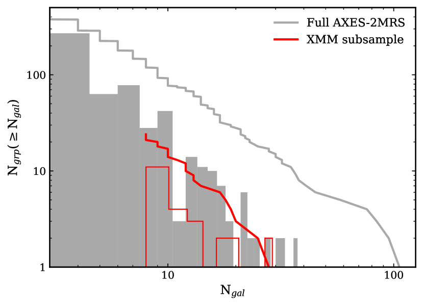
Figure 6: Cumulative distributions (thick histograms) and frequency distributions (shaded and thin histograms of the number of member galaxies (which also traces the group richnesses) for the full AXES-2MRS groups (grey), and the XMM subsample (red).

3.3 Hydrostatic Mass Estimates

The total X-ray-deduced mass inside a radius $r$ assuming hydrostatic equilibrium, a $\beta$-model shape of the gas density, and a polytropic temperature profile ($T(r)\propto N_{\rm gas}^{\gamma-1}$) is (Finoguenov et al., 2001):

$$M(r)=3.7\times 10^{13}\ T(r)\ r\ \frac{3\ \beta\ \gamma\ x^{2}}{1+x^{2}}\,M_{\odot}\ ,$$ (2)

where $x=r/r_{c}$ is the ratio between the radius $r$ and the core radius of the $\beta$-model $r_{c}$ and $\gamma=1.1$. X-ray masses were calculated inside the temperature extraction radius R_kT, and thus $T(r)$ is just the spectroscopic temperature. Elliptical regions were used in the temperature extraction, while we assume a circular symmetry in the mass analysis. We employ the ellipsoidal quadratic mean radius to associate a radius with the temperature extraction region:

$$R_{kT}=\sqrt{\frac{a_{\rm spec}^{2}+b_{\rm spec}^{2}}{2}},$$ (3)

The overdensity of the measurement was estimated as:

$$\Delta=\frac{M(r)}{4\pi/3\,r^{3}\rho_{c}(z)},$$ (4)

where $\rho_{c}(z)$ = $1.37\times 10^{11}E^{2}(z)M_{\odot}/(\rm Mpc)^{3}$ is the critical density of the universe at redshift $z$. Table 6 includes the calculated X-ray masses and their overdensities as well as the rescaled masses at $\Delta$ = 500 and 10000. In rescaling the masses, we used the mean expected concentration following the prescription of Hu & Kravtsov (2014). In addition, we explore our constraints on the concentration of individual halos coming from comparing direct mass estimates at two different overdensities.

3.4 Velocity Dispersion

We choose the gapper velocity dispersion estimator (Beers et al., 1990) as it is preferred in case of a low number of member galaxies. In particular, Beers et al. (1990) favours this method for clusters with less than 15 members. Fig. 6 shows the cumulative distribution of the number of groups ($N_{\rm grp}$) in the full AXES-2MRS, and the XMM subsample, as a function of the number of member galaxies $N_{\rm gal}$, as well as the corresponding frequency distribution.

The velocity dispersion for the groups is calculated as:

$$\sigma_{\rm gap}=\frac{c}{{1+\langle z\rangle}}\,\left(\frac{\sqrt{\pi}}{N(N-1)}\sum_{i=1}^{N-1}w_{i}g_{i}\right),$$ (5)

where $c$ is the speed of light, $N$ is the number of members, $w_{i}$ = $i(N-i)$, $g_{i}$ = $z_{i+1}-z_{i}$ is the pairwise difference between member redshifts, and $\langle z\rangle$ is the mean redshift. The uncertainty on $\sigma_{\rm gap}$ is calculated as:

$$\Delta\sigma_{gap}=\frac{C\sigma_{gap}}{\sqrt{N-1}},$$ (6)

where C=0.91, based on the modelling of Ruel et al. (2014). We adopted the use of the gapper velocity dispersion within the Clean, which removes interlopers and we only use the galaxies inside the $R_{200}$ in the calculation. We report our velocity dispersion measurements of the XMM-Newton subsample in Table 4, and for the full AXES-2MRS catalogue in Table 7.

3.5 Halo Concentration

Our X-ray mass measurements and velocity dispersions constrain the masses of the groups at very different overdensities: the X-ray measurements cover the central part of the group, while spectroscopic members used for the velocity dispersion estimates extend to the virial radius. We take the optical mass measurement from the calibrations of Munari et al. (2013), which linked the $M_{200}$ to the measured $\sigma_{v}$. We seek a value of concentration that describes both X-ray and optical mass measurements. The largest contribution to the error is the statistical error on the velocity dispersion, which is of the order 30% for many groups. This is much larger than any bias associated with the assumption of the hydrostatic equilibrium (HSE, Fabricant & Gorenstein, 1983;Fabricant et al., 1980; Fabricant et al., 1984), especially taking into account the previously found good performance of the HSE technique at the overdensities we use for X-ray mass measurements. The resulting constraints on the concentration are rather uncertain with no group clearly showing deviations from the expected concentration (see Section 4.7 and Table 6).

3.6 Velocity Substructure

We used the Anderson-Darling (AD) normality test (Anderson & Darling, 1954) to split the AXES-2MRS catalogue and the XMM subsample into Gaussian (G) and non-Gaussian (NG) groups and study the effect of velocity substructure on the scaling relations. We followed the procedure outlined in Hou et al. (2009) for applying the AD test. In particular, we calculated the test statistic $A^{2}$ and its (sample size) weighted modification $A^{2*}$, from the ordered velocities of the galaxy group members $x_{i}$, as:

$$A^{2}=-N-\frac{1}{N}\sum_{i=1}^{N}(2i-1)\,\left\{\ln\Phi(x_{i})+\ln\left[1-\Phi\left(x_{N+1-i}\right)\right]\right\}$$ (7)

$$A^{2*}=A^{2}\left(1+\frac{0.75}{N}+\frac{2.25}{N^{2}}\right)\ ,$$ (8)

where $x_{i}\leq x<x_{i+1}$, and $\Phi(x_{i})$ is the cumulative distribution function of the hypothetical underlying Gaussian distribution given as:

$$\Phi(x_{i})=\frac{1}{2}\left[1+\text{erf}\left(\frac{x_{i}-\mu}{\sqrt{2}\sigma_{\rm v}}\right)\right]\ ,$$ (9)

where $\mu$ is the mean velocity of the group, and $\sigma_{\rm v}$ is the velocity dispersion. $A^{2*}$ is then used to compute the significance level $\alpha_{AD}$, used to asses the Gaussianity assumption, as:

$$\alpha_{AD}=a\exp{\left(-\frac{A^{2*}}{b}\right)},$$ (10)

where $a=3.6789468$ and $b=0.1749916$ are numerical fitting parameters taken from Nelson (1998). The percentage of the G groups in AXES-2MRS with at least 8 spectroscopic members is $\sim{77\%}$, consistent with Damsted et al. (2023), who studied dynamics of CODEX clusters, which overlap in X-ray luminosity, but are located at higher redshift.

4 Scaling Relations

4.1 Statistical methods

Primarily, the Python package linmix (Kelly, 2007) was used in the scaling relations of interest in this paper. It was shown by Kelly (2007) that it performs better than other regression estimators (e.g., OLS, BCES(Y—X), and FITEXY) when the measurement errors are large and the sample size is low. Optical $\sigma_{\rm v}$ values naturally exhibit a relatively large uncertainty ($\sim$20-30$\%$), and we perform the scaling relations on a limited-size group sample. The linmix package is based on a hierarchical Bayesian model that approximates a distribution function of the input data points using a mixture of several Gaussian components ($K$). Except for $c_{200}-L_{\rm X}$ relation which has $K=4$ (see Section 4.7), all the scaling relations presented in this section use $K=3$. To better illustrate linmix’s structure, we take the $\sigma_{\rm v}-kT$ relation as an example (see Section 4.4 and figures therein). Essentially, $kT$ and $\sigma_{\rm v}$ are supposed to follow a bivariate log-normal distribution $\mathcal{N}_{2}(\mu,\Sigma)$ with the mean $\mu=(\xi,\eta)$. These values $(\xi,\eta)$ represent the true, yet unobservable means of $\ln{kT}$ and $\ln{\sigma_{\rm v}}$, and the covariance matrix $\Sigma$ contains the errors observed in the logarithmic values of kT and $\sigma_{\rm v}$. The connection between $\xi$ and $\eta$ is established through the conditional probability distribution $P(\eta\,|\,\xi)$ = $\mathcal{N}(A+B\,\xi,S^{2})$. Here, $A$ is the intercept, $B$ is the slope, and $S$ is the Gaussian intrinsic scatter of $\eta$ around the regression line. The exact equation used in the fitting is:

$$\eta=A+B\,x_{i}+S,$$ (11)

where $x=x_{i}+x_{\rm err}$ is the predictor vector of the data points + errors, and $y_{i}=\eta+y_{\rm err}$ is the target vector. The exact fitting formulas used in the scaling relations are listed in Table 2. We use 100 000 Markov chain Monte Carlo (MCMC) iterations within linmix and report the mean of the posterior distribution of the best-fit parameters in Table 3.

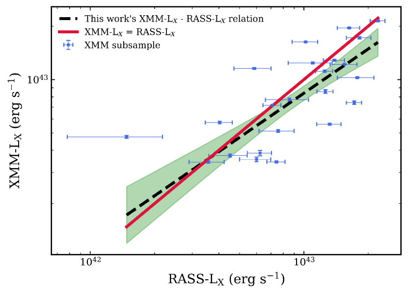
Figure 7: Comparison of AXES-2MRS X-ray luminosity measurements between XMM-Newton and RASS. The dashed line is the best fit. The one-to-one relation between XMM-Newton and RASS is given by the solid line. The shaded region is the 1$\sigma$ uncertainty of the slope and intercept.

Figure 8: MCMC fitting results with one and two-dimensional projections of the posteriors of the XMM-$L_{\rm X}$–RASS $L_{\rm X}$ scaling relation. The vertical line represents the one-to-one relation and corresponds to the red line in Fig. 7. Dark and light contours represent 68$\%$ and 95$\%$ confidence levels, respectively.

Given that we introduce a new sample of galaxy groups and we use Bayesian methods for the analysis of the scaling relations, it is important to separate the contribution of the sample from the difference in the analysis. So, we also apply the orthogonal distance regression (Boggs et al., 1989, ODR). The ODR method fits the data points by minimizing their squared orthogonal distances to the best-fit line. The ODR accounts for measurement errors in the two variables, however, it does not estimate the intrinsic scatter of the relation. For that reason, and the fact that Bayesian methods typically produce wider confidence intervals than frequentist ones, uncertainties of the linmix parameters are somewhat larger. In the following, we present the scaling relation between the XMM-Newton and ROSAT X-ray luminosities ($L_{\rm XMM}-L_{\rm RASS}$). We also present the relation between optical velocity dispersion and each of the X-ray luminosity ($\sigma_{\rm v}-L_{\rm X}$), the X-ray gas temperature ($\sigma_{\rm v}-kT$), and the mass ($\sigma_{\rm v}-M_{10000}$). As well as between the X-ray temperature and luminosity ($kT-L_{\rm X}$) and between the dark matter-halo concentration and luminosity ($c_{200}-L_{\rm X}$).

4.2 Characterisation of AXES X-ray Luminosities

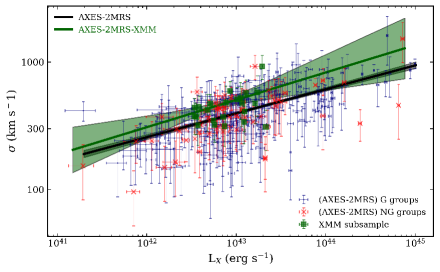
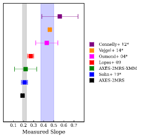
Figure 9: Left panel: Velocity dispersion vs. X-ray luminosity for the full AXES-2MRS systems with at least 5 members and our XMM-Newton subsample. Gaussian and non-Gaussian groups are marked with blue circles and red crosses, respectively. The XMM subsample is marked with filled green squares. Shaded regions are 1$\sigma$ uncertainties. Right panel: Slope comparison for the $\sigma_{\rm v}-L_{\rm X}$ relation with the literature. The grey-shaded region is the self-similar expectation calibrated according to the X-ray emissivity in the band-limited ($0.1-2.4$ keV) low-temperature ($0.7-3.0$ keV) range. While the blue-shaded region is for the bolometric luminosity. (* refers to relations originally expressed as $L_{\rm X}-\sigma_{\rm v}$ and was inverted for comparability).

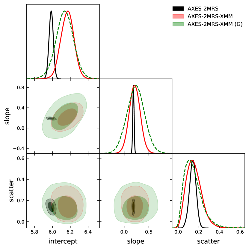
Figure 10: MCMC fitting results with one and two-dimensional projections of the posteriors of the $\sigma_{\rm v}-L_{\rm X}$ scaling relation. Other details are the same as Fig. 8.

Since AXES presents new estimates of X-ray luminosities, measured using large sky areas, it is important to assess the quality of these estimates, using better X-ray observations available with XMM-Newton. In the computation of X-ray luminosities, we select the band to report the luminosity to be consistent with other studies, 0.1–2.4 keV. The flux measurement is performed using the 0.5–2.0 keV band for both ROSAT and XMM-Newton data. In the calculation of the luminosity, a K-correction using the redshift of the source, temperature estimate using the same $L-T$ relation, and a band difference between observed 0.5–2 keV (used for the flux measurements) and the rest-frame 0.1-2.4 keV (used for $L_{\rm X}$) is made. There are some subtle differences, as in RASS data we use the full flux, and in XMM-Newton, we remove the contribution of point sources. Also, with XMM-Newton data, the flux apertures capture more precisely the contribution of the group, thus avoiding an extra source of scatter due to confusion. Thus, even with a smaller sample size, XMM-Newton data on luminosities deliver improvements on the association of X-ray emission with the galaxy group. Both RASS and XMM-Newton fluxes are extrapolated to the estimated $R_{500}$ radius following the procedure described in Finoguenov et al. (2007). RASS data requires no extrapolation, while these aperture corrections to XMM-Newton fluxes are within 20%. However, a difference in the spatial coverage of the source introduces an additional source of scatter. The correspondence between the X-ray luminosity measurements between XMM-Newton and RASS is illustrated in Fig. 7, Fig. 8, and detailed in Table 3. The relation is close to the one-to-one relation, and the main effect we see is a 40% scatter in the luminosity estimates, which we attribute to be a characteristic of the quality of survey-type measurement of RASS.

4.3 Velocity Dispersion – X-ray Luminosity Relation

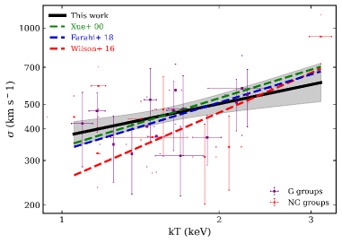
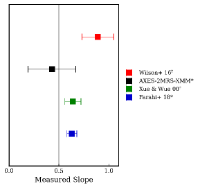
Figure 11: Left panel: Velocity dispersion vs. temperature for the XMM-Newton subsample used in this work in comparison with the literature. Gaussian and non-Gaussian groups in our sample are represented by purple squares and red crosses, respectively. The grey transparent band is 1$\sigma$ confidence interval for the slope and intercept. Right panel: Comparison of the slope of the $\sigma_{\rm v}-kT$ relation with the literature. The grey solid line is the theoretical self-similar expectation.* refers to works using Bayesian linear regression while $\dagger$ refers to works using ODR. The slope of Wilson et al. (2016) is subject to a potential bias discussed in Farahi et al. (2018).

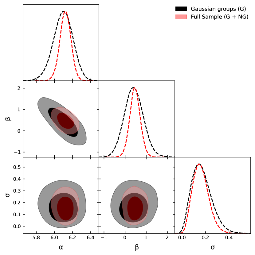
Figure 12: MCMC fitting results with one and two-dimensional projections of the posteriors of the $\sigma_{\rm v}-kT$ scaling relation. Other details are the same as Fig. 8.

Since no selection criteria were applied on $\sigma_{\rm v}$ in our XMM-Newton subsample, we examine the $\sigma_{\rm v}-L_{\rm X}$ relation, instead of $L_{\rm X}-\sigma_{\rm v}$, and compare it to the relation of the full AXES-2MRS catalogue (for a detailed discussion on the choice, see Kelly, 2007). We are particularly interested in comparing the constrained intrinsic scatters to assess the effect of sources of contamination (point sources, nearby groups, etc.) on the $\sigma_{\rm v}-L_{\rm X}$ relation, due to XMM-Newton’s higher sensitivity to those compared to ROSAT. We present our scaling relation work and compare it to the literature results on the group scale in Fig. 9, with the one and two-dimensional projections of the posteriors of the parameters shown in Fig. 10. Our result for the full XMM-sample ($\sigma_{\rm v}\propto$ $L_{\rm X}^{0.22\pm 0.11}$) is in agreement with the calibration of the self-similar expectation based on the X-ray emissivity behaviour in the 0.1-2.4 keV energy band and 0.7-3.0 keV temperature range (see the right panel in Fig. 9 for our result in comparison with the literature). Lovisari et al. (2021) presents an argument about the truly expected slope of this relation based on the behaviour of the X-ray emissivity in the low-temperature regime. They claim that instead of $L_{\rm X}\propto\sigma_{\rm v}^{4}$, the scaling should follow $L_{\rm X}\propto\sigma_{\rm v}^{3+2\gamma}$, where $\gamma$ is a constant determined based on the temperature range, energy band, and metallicity (see Table 1 in Lovisari et al., 2021). Indeed, the most deviating results are obtained for galaxy groups at lower X-ray luminosities, compared to our sample. We detail the parameters of the $\sigma_{\rm v}-L_{\rm X}$ relation in Table 3. We notice almost no change in the scatter of both XMM and ROSAT relations, which we attribute to the level of intrinsic scatter being much larger than the scatter between XMM-Newton and RASS luminosities. Although there is a noticeable difference in the normalization of the scaling relation between RASS and XMM samples, once we retain only the high-quality measurements of velocity dispersion by limiting the sample to that of at least 8 spectroscopic members, the difference disappears. This means that our XMM-Newton subsample is representative of the 8 or more member AXES groups, while the full catalogue is somewhat different. Moreover, we investigate the effect of the number of spectroscopic members on the relation, and we find that adding poor galaxy groups (${N_{\rm gal}}<8$) does not affect the quality of the fit in terms of the statistical errors and the intrinsic scatter (on the 1-$\sigma$ level). Up to our level of precision, there is no clear evidence of substructure (NG) deviations in the $\sigma_{\rm v}-L_{\rm X}$ relation as shown in Table 3. Additionally, we matched the AXES-2MRS sample and the XMM-Newton subsample with The Third Cambridge Catalog (3C) and its revised version (3CR) within 5 arcmin to test whether including galaxy groups with an active radio AGN changes the scaling relations. We removed a total of 6 systems from the full AXES-2MRS sample and 1 system from the XMM subsample, and we did not find any noticeable change in the scaling relations, concluding that ongoing AGN activity is not immediately seen in the group properties. In the subsequent analysis, we no longer split the sample based on the radio properties.

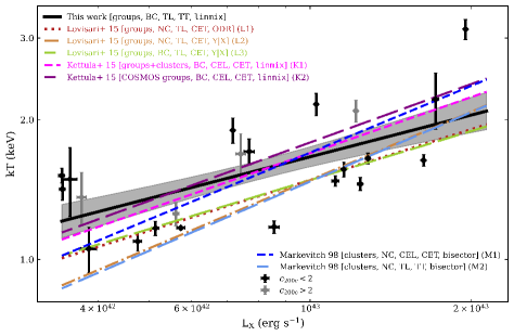
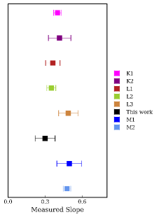
Figure 13: Left panel: Temperature vs. X-ray luminosity for the XMM-Newton subsample used in this work (black solid line) in comparison with the literature. BC and NC indicate bias-corrected and non-corrected relations, respectively. TL and CEL are total and core-excised $L_{\rm X}$, respectively. TT and CET are total and core-excised $kT$, respectively. The type of the sample used and the regression method are also indicated (see section 4.5 for more details). Grey and black points are high and low concentration groups, respectively, defined at $c_{200}=2$. Shaded region is the 1-$\sigma$ uncertainty. Right panel: Comparison of the slope of the $kT-L_{\rm X}$ relation with the literature. Slope labels are the same as relation labels from the left panel. Only band-limited $L_{0.1-2.4}$ relations are considered.

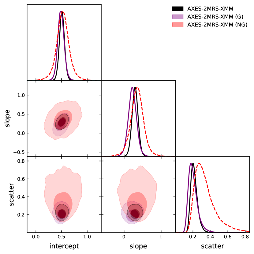
Figure 14: MCMC fitting results with one and two-dimensional projections of the posteriors of the $kT-L_{\rm X}$ scaling relation. Other details are the same as Fig. 8.

Tracking the efforts done studying the $\sigma_{\rm v}-L_{\rm X}$ relation, we find that Sohn et al. (2019) used a sample of 74 groups from the COSMOS survey (Finoguenov et al., 2007; Gozaliasl et al., 2019) and reported a scaling of the form $\sigma_{\rm v}\propto L_{\rm X}^{0.21\pm 0.03}$. Their sample suffered from anomalously low velocity dispersion values so they reduced their sample to 7 velocity dispersion bins and fitted them to get the above result. Notably, they state that the intrinsic scatter of their relation came high, however, they do not report a specific value. Lopes et al. (2009b) used a (group + cluster) sample of 97 systems from the NoSOCS-SDSS survey (Lopes et al., 2009a) and reported a result of the form $\sigma_{\rm v}\propto L_{\rm X}^{0.27\pm 0.03}$ with an intrinsic scatter ($S_{\mathrm{ln}Y|X}$) of $0.29\pm 0.03$. Osmond & Ponman (2004) was one of the earliest efforts in constraining this relation on the group scale. They used ROSAT data for a group sample of 60 systems and reported a result of the form $\sigma_{\rm v}\propto L_{\rm X}^{0.43\pm 0.11}$. Next, Vajgel et al. (2014) used a small sample of 14 groups from the X-Boötes survey (Murray et al., 2005) and reported a relation of the form $\sigma_{\rm v}\propto L_{\rm X}^{0.46\pm 0.01}$ and intrinsic log-normal scatter of 0.3. Lastly, Connelly et al. (2012), using a sample of 38 high redshift X-ray groups with luminosities around $10^{42}$ ergs s^-1 measured using deep XMM-Newton observations, derived a scaling of the form $\sigma_{\rm v}\propto L_{\rm X}^{0.56\pm 0.18}$, with $L_{\rm X}$ estimates similar to those obtained in the COSMOS field, so the difference is mainly in the covered luminosity range. We report the least intrinsic scatter in the $\sigma_{\rm v}-L_{\rm X}$ relation in the literature so far with a value of $0.15\pm 0.07$. We note that the original relations reported in Sohn et al. (2019); Osmond & Ponman (2004); Vajgel et al. (2014); Connelly et al. (2012) were in the form $L_{\rm X}-\sigma_{\rm v}$, while we inverted them for the slope comparison.

4.4 Velocity Dispersion – X-ray Temperature Relation

We study the $\sigma_{\rm v}-kT$ for the full XMM sample of 24 groups we have (the effect of adding the dynamically complex 2MRS ID: 5089 system is explored later in this section). The importance of these two observables arises as they are independent baryonic tracers for the depth of the group potential. In the absence of non-gravitational heating, one expects the scaling to go as $\sigma_{\rm v}\propto T^{0.5}$. We report a consistent relation of the form $\sigma_{v}\propto T^{0.42\pm 0.24}$. Detailed parameter estimations for the $\sigma_{\rm v}-kT$ relation are summarised in Table 3. The role of the velocity substructure in enhancing the scatter is marginally supported by the data with the Gaussian (G) groups and the full sample having 40% lower intrinsic scatter than the non-Gaussian (NG) groups. Fig.12 shows the one and two-dimensional projections of the posteriors of the relation.

We consider both group and group + cluster samples when comparing our fit to the literature, with the results on the slope summarised in Fig. 11. Xue & Wu (2000) studied a low-redshift sample of 274 groups and clusters with $kT<$ 10.1 keV, and found a relation of the form $\sigma_{\rm v}\propto T^{0.64\pm 0.08}$ using the ODR method with no characterization of intrinsic scatter. Our data is more uniform because all the X-ray observations used were obtained from the same instrument, and we have more control over the velocity dispersion values as they were all computed using the same (gapper) estimator. In contrast, they assembled their X-ray and spectroscopic samples from 20 different sources. Using a total of 19 groups + clusters with $kT<$ 5.5 keV taken from the XMM Cluster Survey (Mehrtens et al., 2012), Wilson et al. (2016) reported a steep relation of the form $\sigma_{\rm v}\propto T^{0.86\pm 0.16}$. Lastly, Farahi et al. (2018) used a 138 group + cluster sample selected from the XXL survey. X-ray temperatures ($kT<$ 6.5 keV) were taken from the XXL analysis of Adami et al. (2018), and spectroscopic data for galaxies were obtained from 7 different literature sources. They report a relation in the form $\sigma_{\rm v}\propto T^{0.63\pm 0.05}$. Despite the formal difference in the slope values, as illustrated in Fig.11, all the fits are broadly consistent with our data points. Therefore, obtaining a different slope of the scaling relation might be a result of a different sampling of the data. Exploring larger datasets and understanding the covariance of the scatter with the group properties affecting the selection is needed to establish a full picture.

4.5 X-ray Temperature – Luminosity Relation

The soft-band X-ray luminosity and temperature are two X-ray observables obtained with minimal covariance. In our analysis, X-ray temperatures were obtained from spectral modelling of the X-ray observations. In contrast, X-ray luminosities were derived from the flux measurements in the 0.5–2 keV energy band, which, at the redshifts of this study, are primarily sensitive to gas density and metallicity. Accordingly, the $kT-L_{\rm X}$ relation is one of the most studied relations in the literature. The gravitational self-similar expectation is $L_{\rm bol}\propto T^{2}$, where $L_{\rm bol}$ is the bolometric luminosity (e.g., Böhringer et al. (2012), and references therein). However, the expected behaviour of the band-limited [0.1-2.4 keV] relation is $L_{0.1-2.4}\propto T^{1.5+\gamma}$ with $\gamma=-0.04$ for a typical metal abundance of $Z=0.3\,Z_{\odot}$ and a temperature range of 0.4–3.0 keV(Lovisari et al., 2021). Thus, the slope of the $kT-L_{\rm X}$ relation is expected to be $\sim$ 0.67. We report a relation of the form $kT\propto L_{\rm X}^{0.3{\pm}0.08}$ for the XMM-Newton subsample representing AXES-2MRS. We show our relation, together with that of Kettula et al. (2015); Lovisari et al. (2015); Markevitch (1998) in Fig. 13. To ensure an in-depth comparison, we list several properties of the literature relations in the left panel of the figure. In particular, we specify whether the relation is based on a group, cluster, or group + cluster sample. We also indicate whether it employs a selection bias correction (BC) or not (NC), and specify whether the central regions were excluded in estimating $L_{\rm X}$ (core excised, CEL) or the total $L_{\rm X}$ was used (TL). Furthermore, total (TT) vs. core-excised (CET) temperature is clarified together with the regression method. These acronyms are summarised in Table. 1. To correct for the sampling bias of our XMM-Newton subsample, we provide a detection vector to linmix to take into account the distribution of source over the luminosity, where we set temperatures for the systems without XMM-Newton temperature measurements to its upper limit of 20 keV. We do not find differences in the results obtained without a detection vector, which illustrates that the sampling bias is negligible.

Table 1: Acronyms used in the $kT-L_{\rm{X}}$ relation

Acronym	Definition
BC	Selection-bias corrected
NC	Selection-bias non-corrected
CEL	Core-excised X-ray luminosity
TL	Total X-ray luminosity
CET	Core-excised X-ray temperature
TT	Total X-ray temperature

The literature scaling relations shown in Fig. 13 are detailed as follows: firstly, Lovisari et al. (2015) compiled a group sample by applying a flux limit of $F_{0.1-2.4}=5\times 10^{-12}$ erg s^-1cm^-2 and two redshift cuts ($0.01<z<0.035$) to the northern ROSAT all-sky galaxy cluster survey (Böhringer et al., 2000, NORAS) and the ROSAT-ESO flux-limited X-ray galaxy cluster survey (Böhringer et al., 2004, REFLEX) catalogues. The resulting 23-group sample span a similar temperature ($0.85<kT<2.8$ keV) and band-limited luminosity range ($0.4<L_{\rm X}<5.3\times 10^{43}$ erg s^-1) as our XMM-subsample, and uses total luminosities and core-excised temperatures. Moreover, multiple regression methods were used, and in Fig. 13 we show the relation using two of them (ODR and BCES Y—X) as well as the BC and NC relations. On the other hand, Kettula et al. (2015) produced the $L_{\rm X}-kT$ relation based on a compiled sample of 12 low-mass clusters from the XMM-CFHTLS survey (Mirkazemi et al., 2015), 10 low-mass systems from the COSMOS field (Kettula et al., 2013), and 48 high-mass clusters from the Canadian Cluster Comparison Project (Hoekstra et al., 2015; Mahdavi et al., 2013, CCCP). The combined sample has a temperature and luminosity range of $1-12$ keV, and $10^{43}-10^{45}$ erg s^-1, respectively. In Fig. 13, we show their relation with the combined group + cluster sample and that with only the low-mass COSMOS systems since the latter shows greater similarity in the parameter ranges with our study. Nevertheless, we note that they exclusively used CEL and CET. As a high-mass reference, Markevitch (1998) used a low-redshift ($0.04<z<0.09$) 35-cluster sample selected from RASS that excludes systems with $kT\leq 3.5$ keV and has a mean TL of $\sim 3.86\times 10^{44}$ erg s^-1. We show their relation using CEL and CET as well as that using TL and TT. In the right panel of Fig. 13, we separately compare the slope of the relation with the mentioned works.

Fig. 13 indicates that all the previous studies of the $T-L_{\rm X}$ relation in groups are consistent with our data and differences in the slope can be attributed to the selection effects or the fitting method used. All these slopes are shallower than the cluster slope of Markevitch (1998), indicating that the groups are hotter than expected from the extrapolation of the cluster relation, which can be attributed to the effect of feedback, to higher concentration, or an earlier formation epoch. The effect of feedback on the scaling relations is largely removed when using total mass measurements, instead of temperature, while the effect of the difference in the concentration would remain in those studies. This motivates us to consider the scaling relations using the total mass and to measure the concentration for our sample.

Table 2: Fitting formulas of the scaling relations.

Relation	Fitting formula
$L_{\rm XMM}-L_{\rm RASS}$	$\ln(L_{\rm XMM}/10^{43}$ erg s${}^{-1})=A+B\ln(L_{\rm RASS}/10^{43}$ erg s${}^{-1})+S_{\mathrm{ln}Y|X}$
$\sigma_{\rm v}-L_{\rm X}$	$\ln(\sigma_{\rm v}$ km s${}^{-1})=A+B\ln(L_{\rm X}/10^{43}$ erg s${}^{-1})+S_{\mathrm{ln}Y|X}$
$\sigma_{\rm v}-kT$	$\ln(\sigma_{\rm v}$ km s${}^{-1})=A+B\ln(kT/1.5$ keV) + $S_{\mathrm{ln}Y|X}$
$kT-L_{\rm X}$	$\ln(kT$ keV${}^{-1})=A+B\ln(L_{\rm X}/10^{43}$ erg s${}^{-1})+S_{\mathrm{ln}Y|X}$
$\sigma_{\rm v}-M_{10000}$	$\ln(\sigma_{\rm v}$ km s${}^{-1})=A+B\ln(M_{10000}/10^{13}M_{\odot})+S_{\mathrm{ln}Y|X}$
$c_{200}-L_{\rm X}$	$\ln(c_{200})$ = $A$ + $B$ $\ln(L_{\rm X}/8\times 10^{42}$ erg s-1) + $S_{\mathrm{ln}Y|X}$

Table 3: Scaling relations.

Relation	Sample	linmix			ODR
		intercept	slope	scatter	intercept	slope
		$A$	$B$	$S_{\mathrm{ln}Y|X}$	$A$	$B$
$L_{\rm XMM}-L_{\rm RASS}$	Full XMM (23)	-0.18 $\pm$ 0.1	0.83 $\pm$ 0.19	0.43 $\pm$ 0.08	-0.31 $\pm$ 0.12	1.56 $\pm$ 0.31
$\sigma_{\rm v}-L_{\rm X}$	AXES-2MRS ($N_{\rm gal}>4$) (252)	5.99 $\pm$ 0.02	0.19 $\pm$ 0.01	0.14 $\pm$ 0.03	6.01 $\pm$ 0.02	0.19 $\pm$ 0.01
	AXES-2MRS ($N_{\rm gal}>7$) (134)	6.03 $\pm$ 0.03	0.17 $\pm$ 0.02	0.17 $\pm$ 0.04	6.1 $\pm$ 0.03	0.17 $\pm$ 0.01
	AXES-2MRS ($N_{\rm gal}>$ 7, G) (102)	6.07 $\pm$ 0.03	0.17 $\pm$ 0.02	0.16 $\pm$ 0.04	6.1 $\pm$ 0.03	0.17 $\pm$ 0.01
	AXES-2MRS ($N_{\rm gal}>$ 7, NG) (32)	6.06 $\pm$ 0.06	0.17 $\pm$ 0.05	0.23 $\pm$ 0.08	6.09 $\pm$ 0.05	0.16 $\pm$ 0.04
	Full XMM (23)	6.17 $\pm$ 0.07	0.21 $\pm$ 0.11	0.15 $\pm$ 0.07	6.19 $\pm$ 0.06	0.22 $\pm$ 0.09
	XMM (G) (14)	6.14 $\pm$ 0.1	0.23 $\pm$ 0.18	0.14 $\pm$ 0.09	6.14 $\pm$ 0.05	0.23 $\pm$ 0.09
	XMM (NG)	6.17 $\pm$ 0.2	0.17 $\pm$ 0.27	0.41 $\pm$ 0.24	6.25 $\pm$ 0.12	0.23 $\pm$ 0.16
$\sigma_{\rm v}-kT$	Full XMM (24)	6.11 $\pm$ 0.07	0.43 $\pm$ 0.24	0.15 $\pm$ 0.07	6.12 $\pm$ 0.05	0.44 $\pm$ 0.18
	XMM (G) (15)	6.09 $\pm$ 0.08	0.29 $\pm$ 0.41	0.16 $\pm$ 0.09	6.1 $\pm$ 0.05	0.28 $\pm$ 0.2
	XMM (NG) (9)	6.1 $\pm$ 0.18	0.48 $\pm$ 0.54	0.39 $\pm$ 0.23	6.16 $\pm$ 0.11	0.52 $\pm$ 0.31
$kT-L_{\rm X}$	Full XMM (23)	0.51 $\pm$ 0.05	0.3 $\pm$ 0.08	0.21 $\pm$ 0.04	0.4 $\pm$ 0.04	0.36 $\pm$ 0.07
	XMM (G) (14)	0.49 $\pm$ 0.07	0.22 $\pm$ 0.12	0.2 $\pm$ 0.06	0.42 $\pm$ 0.04	0.16 $\pm$ 0.08
	XMM (NG) (9)	0.53 $\pm$ 0.14	0.35 $\pm$ 0.19	0.35 $\pm$ 0.15	0.43 $\pm$ 0.07	0.47 $\pm$ 0.12
$\sigma_{\rm v}-M_{10000}$	Full mass sample (30)	6.1 $\pm$ 0.06	0.13 $\pm$ 0.05	0.12 $\pm$ 0.06	6.15 $\pm$ 0.04	0.12 $\pm$ 0.04
	XMM (G) (15)	6.13 $\pm$ 0.09	0.22 $\pm$ 0.18	0.14 $\pm$ 0.08	6.13 $\pm$ 0.05	0.13 $\pm$ 0.06
	XMM (NG) (9)	6.23 $\pm$ 0.18	0.31 $\pm$ 0.26	0.34 $\pm$ 0.22	6.31 $\pm$ 0.11	0.34 $\pm$ 0.13
$c_{200}-L_{\rm X}$	Full $c_{200}$ sample (24)	–0.12 $\pm$ 0.96	0.15 $\pm$ 5.37	0.76 $\pm$ 0.31	9.51 $\pm$ 17.75	–1.51 $\pm$ 3.55

4.6 Velocity Dispersion – Mass Relation

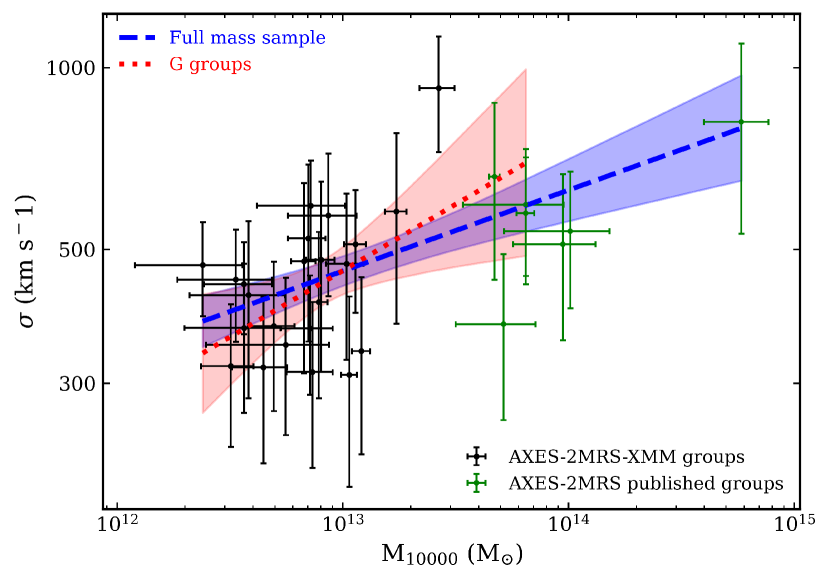
Figure 15: Velocity dispersion vs. mass within a sphere of overdensity $10^{4}$ relative to the critical density of the Universe. Blue dashed and red dotted lines represent the scaling relation of our full mass sample (see Section 4.6 and the Gaussian subsample, respectively. Black and green points are our XMM-Newton subsample and AXES-2MRS published groups, respectively.

Figure 16: MCMC fitting results with one and two-dimensional projections of the posteriors of the $\sigma_{\rm v}-M_{10000}$ scaling relation. Other details are the same as Fig. 8.

As most of our mass measurements correspond to a high overdensity, finding a correspondence to our measurement of velocity dispersion, which traces virial mass, is sensitive to halo concentration. In this section, we consider the scatter in the estimate of the central mass this effect introduces and include an effect of complexity in the velocity dispersion profile into consideration. The obtained relation for our mass sample is shown in Fig.15 while the details of the fitting parameters and the one and two-dimensional posteriors are presented in Table 3 and Fig. 16, respectively. While we have concentrated on the XMM-Newton analysis on galaxy group scales, an analysis of AXES-2MRS clusters can be readily found in the literature (e.g. Schellenberger & Reiprich, 2017). To improve on the mass coverage, we included previously published results from the HIFLUGCS cluster sample (Schellenberger & Reiprich, 2017), in overlap with our velocity dispersion measurements. We report a nearly flat relation for the full mass sample of $\sigma_{\rm v}\propto M_{10000}^{0.13\pm 0.05}$. The deviations of the slope from the $M^{1/3}$ expectation can be explained either if the contribution of the non-thermal pressure to the mass estimate at the overdensities of 10000 is high in galaxy groups, or if our sample is dominated by the low concentration systems, which we explore below. Splitting the systems, based on the Gaussianity of velocity dispersion, does not lead to any detectable changes in the parameters of this scaling relation.

4.7 Concentration – X-ray Luminosity Relation

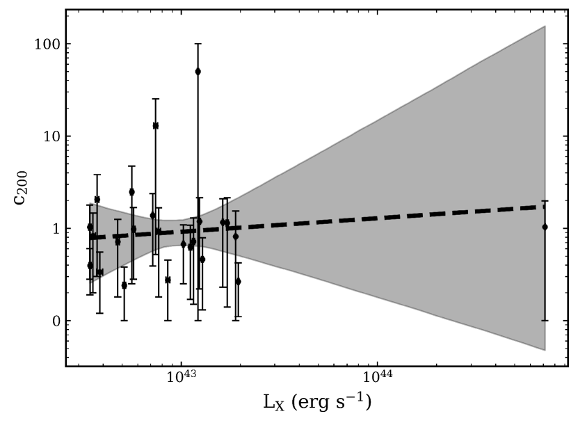
Figure 17: Halo concentration vs. X-ray luminosity for the $c_{200}$ sample used in this work.

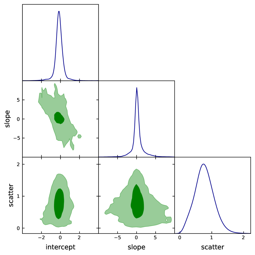
Figure 18: MCMC fitting results with one and two-dimensional projections of the posteriors of the $c_{200}-L_{\rm X}$ scaling relation. Other details are the same as Fig. 8.

Owing to the hypersensitivity of the concentration calculation to variations in the velocity dispersion, coupled with the presence of relatively large errors in our velocity dispersion measurements, approximately on the order of 20-30%, the determination of the concentration parameter poses a significant challenge. As a result, we were only able to confidently constrain the concentration of 22 systems within our XMM-Newton subsample (see Table 6). Additionally, due to the intricate nature of this analysis, we could extend our concentration determinations to only two systems from previously published datasets (Group IDs: 6041 and 6093). The result of the $c_{200}-L_{\rm X}$ scaling relation is shown in Figs. 17 and 18 and the details of the parameters are shown in Table 3. We used $K=4$ Gaussian components in fitting this relation with linmix instead of 3 (see Section 4) as it was found to increase the significance level of the parameters by a factor of 2. Remarkably, we measured a low halo concentration across the majority of systems within our XMM subsample, with values below 1. In performing the linear regression analysis, as an input on concentration we have described the probability distribution of concentrations in the expected range between 1 and 10 using a log-normal distribution, as most points have asymmetric profiles of the probability distribution function, and of relevance is the correct estimate of this probability in the range of expected solution. Our result on the slope of the scaling of $-0.12\pm 0.96$ broadly agrees with the expectations based on the numerical modelling of the $c_{\rm 200}-M$ relation on the scales of groups and clusters of galaxies.

We report a logarithmic intrinsic scatter on the concentration of $S(\ln c_{200})=0.76\pm 0.31$. Within errors, our mean value is slightly higher than the results on the $c_{\rm 200}-M$ relation from cosmological simulations of $S(\ln c_{200})\approx 0.33$ (Wechsler et al., 2002; Neto et al., 2007; Macciò et al., 2007, 2008; Bhattacharya et al., 2013; Child et al., 2018). Observational efforts on the $S(\ln c_{200})$ parameter, despite being limited and mostly inferred from the $c_{\rm 200}-M$ relation, show a fair agreement with the simulations (e.g., Wojtak & Łokas, 2010; Amodeo et al., 2016; Umetsu et al., 2020). In particular, Wojtak & Łokas (2010) assembled a low-redshift ($z<0.1$) sample of 41 relaxed and rich ($N_{\rm gal}\geq 70$) clusters from the NASA/IPAC Extragalactic Database (NED) and The WIde field Nearby Galaxy cluster Survey (Cava et al., 2009, WINGS). The median mass of the sample is $5\times 10^{14}M_{\odot}$ and the median concentration is 7. They report an intrinsic scatter of $S(\ln c_{200})=0.35$. On the other hand, Amodeo et al. (2016) used a high-redshift ($z\geq 0.4$) sample of 47 clusters collected from the Chandra public archive and represents the high-mass end of the cluster population with a median mass of $1.3\times 10^{15}M_{\odot}$. They report a mean log-normal scatter of $S(\ln c_{200})=0.32$. Finally, Umetsu et al. (2020) reported a low upper limit on $S(\ln c_{200})$ of 0.24 using the X-ray selected XXL cluster sample (Adami et al., 2018). They claim that this low scatter can be attributed to a selection bias related to the dynamical state of the clusters or a result of overestimation of the $c_{200}$ measurement errors.

It is important to note that Amodeo et al. (2016) has shown that the intrinsic scatter decreases with increasing mass. In fact, the weak but systematic anti-correlation of mass and intrinsic scatter is also supported by the simulation work of Neto et al. (2007). Given the low masses of our XMM-Newton subsample, this effect could potentially explain the relatively high mean value of the scatter. Additionally, a larger sample with higher luminosity and concentration ranges can improve the significance of the scatter measurement.

5 Conclusions and Summary

In this work, we presented a new catalogue of AXES-2MRS galaxy groups, which has a selection based on the baryonic content at $M_{500}$ and we examined its properties. We have significantly enhanced the representation of the under-explored low-redshift low-luminosity galaxy groups. In addition, our sample is prevalent in low-mass systems ($<$ 10${}^{14}M_{\odot}$, see Table 6), which enhances the completeness of the galaxy group catalogues, potentially addressing the longstanding problem of missing faint low-mass systems.

The main parameter in common between various subsamples studied here is velocity dispersion. We find the main sample to exhibit a comparable scaling relation between the X-ray luminosity and the velocity dispersion, and in particular, to exhibit a similar scatter. The value of the scatter is high, which is in agreement with the conclusion of Damsted et al. (2023) that the scatter at $z<0.15$ is very large. We can see that using our measurements of intra-group medium temperatures does not resolve this problem, and the scatter is still large. Our use of masses, as opposed to temperature, reduces the scatter, which indicates that feedback effects contribute significantly to the scatter. Our reported $\sigma_{\rm v}-kT$ relation is also marginally flatter than the self-similar expectation, which also points to either the importance of non-gravitational heating or the effect of halo concentration. Our analysis of the $c_{200}-L_{\rm X}$ relation reveals a large intrinsic scatter that we deem representative of galaxy groups. Thus, we conclude that both feedback and halo concentration are at the root of the large scatter of properties of X-ray groups. We believe that a combination of large scatter and group selection can explain differences in the mean scaling relations for galaxy groups, as all published relations pass through some of the points presented in this study. The main question that remains open is what is the right balance of groups to be included in the samples of X-ray properties.

We note a similarity in the slope and normalization of the scaling relation between the velocity dispersion and X-ray luminosity between AXES-2MRS galaxy group sample and the distant COSMOS sample, which is obtained using a similar X-ray detection technique. Besides, the XMM-Newton-observed subsample is comparable to the full AXES-2MRS catalogue in this relation and can be safely held as representative of the full AXES-2MRS sample.

Using linmix with intrinsic scatter, the fitting parameters come out consistent with our results using orthogonal distance regression. The reported uncertainties of linmix are however larger by a factor of 1.5-2. This might help resolve previously found tensions in the fit parameters obtained without the intrinsic scatter. As we have demonstrated the scatter of the scaling relations is a meaningful parameter that allows one to access the physics of galaxy groups.

As discussed in the paper, the differences in the literature results on the scaling relations might be associated with the selection of the sample. Our study has employed the largest angular scales ever considered in X-ray source identification. Our results on the scaling relations are within the difference between the literature results, which limits the scope of contribution from the ”known unknowns”. The number of AXES sources combined with the spatial scales employed in searching for the X-ray emission approaches the source confusion limit. While further detailed studies of AXES sources will be beneficial, deeper surveys will have to use smaller spatial scales in searching for X-ray emission, leading to different selection effects. With the advances in hydrodynamical simulations, modelling of the X-ray emission from the outskirts of groups and clusters of galaxies becomes reliable, which makes AXES the most suitable sample for comparison to simulations.

Appendix A Details of the XMM-Newton Observations

Table 4 lists the optical parameters of our XMM-Newton subsample. The positions (RA and Dec) correspond to the X-ray peak emission centres taken as a centroid of a wavelet reconstruction of the 0.5–2 keV image on scales 0.5-4 arcmin. Also shown are the median group redshifts, the optical line-of-sight velocity dispersions determined using the gapper method, and the number of member galaxies.

Table 4: XMM-Newton subsample of AXES-2MRS groups.

Group ID​​​​	RA	Dec	$z_{\rm{med}}$	$\sigma$v	$N_{\rm{gal}}$
2MRS	(J2000)	(J2000)		(km s-1)
361	16.853	32.399	0.016	370 $\pm$ 83	18
505	21.445	–1.395	0.0171	438 $\pm$ 76	29
827	35.780	42.986	0.0197	510 $\pm$ 117	17
859	36.401	36.961	0.0353	480 $\pm$ 167	8
1571	61.642	30.379	0.0179	370 $\pm$ 103	12
1830	74.732	–0.484	0.0144	320 $\pm$ 85	13
2009	86.370	–25.936	0.0388	925 $\pm$ 201	19
2161	96.162	–37.337	0.0329	569 $\pm$ 151	13
2533	315.436	–13.311	0.0278	409 $\pm$ 125	10
2541	117.844	50.202	0.0229	521 $\pm$ 170	9
2657	125.154	21.072	0.017	373 $\pm$ 104	12
3551	164.543	1.612	0.0405	339 $\pm$ 110	9
3718	170.612	24.296	0.027	478 $\pm$ 166	8
4050	182.018	25.239	0.023	319 $\pm$ 98	10
4808	202.351	11.765	0.0239	347 $\pm$ 101	11
5089	210.908	–33.983	0.0139	238 $\pm$ 66	12
5841	244.338	34.903	0.0303	313 $\pm$ 96	10
5914	247.417	40.826	0.0318	591 $\pm$ 111	25
6015	254.498	27.858	0.0345	309 $\pm$ 108	8
6116	260.202	–1.039	0.0286	538 $\pm$ 137	14
6407	281.827	–63.332	0.015	471 $\pm$ 83	28
6666	304.458	–70.819	0.0131	420 $\pm$ 137	9
6916	316.840	–25.459	0.0359	577 $\pm$ 201	8
7427	348.942	–2.389	0.0234	473 $\pm$ 145	19
7727	181.04	20.293	0.0248	445 $\pm$ 94	20

In Table 5, we provide a detailed summary of the observations for our XMM subsample. The table includes Group ID (XMM-Newton group identifier), OBS-ID (XMM-Newton observation identifier), DATE-OBS (date of the observation), Clean-EXP (clean exposure time), kT (X-ray gas temperature), and $L_{\rm X}$ (0.1-2.4 keV X-ray luminosity). It also includes a_spec, b_spec, and $\theta$ which are the semi-major axis, semi-minor axis, and position angle of the elliptical extraction regions used in the spectral analysis, respectively (see the green regions in Fig. 19).

Table 6 complements Table 5 with more X-ray properties obtained from the XMM-Newton observations. In particular, it contains the details of the surface brightness profile fitting using a single $\beta$-model and mass estimates. The columns are $\beta$ (slope of the surface brightness profile), R_kT (the outer radius of the initial mass estimate), $\Delta_{kT}$ (the overdensity of the measurement at R_kT), M${}_{\Delta_{R_{kT}}}$ (the mass estimate at the initial overdensity $\Delta_{kT}$), R_C (the core radius of the $\beta$ model), DS (the distance scale), M₁₀₀₀₀ (mass estimate at the overdensity covered by the data), and c₂₀₀ (halo concentration).

Table 5: XMM observations and basic properties of AXES-2MRS.

Group ID	OBS-ID	DATE-OBS	Clean-EXP	$k\,T$	$L_{\rm X}$	$a_{\rm spec}$	$b_{\rm spec}$	$\theta$
2MRS	XMM-Newton	(UTC)	(ks)	(keV)	(1043 erg s-1)	(arcmin)	(arcmin)	​​​(deg)
361	0551720101	2008-07-01	24.1	1.898 $\pm$ 0.119	0.716 $\pm$ 0.004	4.5	3.5	82.9
505	0743700201	2015-01-09	69.4	1.417 $\pm$ 0.077	0.344 $\pm$ 0.004	2.7	1.4	33.9
827	0002970201	2002-02-05	13.5	2.159 $\pm$ 0.121	1.027 $\pm$ 0.009	4.7	3.9	277.7
859	0863880401	2020-07-21	15.1	1.708 $\pm$ 0.110	0.769 $\pm$ 0.02	2.8	2.2	278.4
1571	0883620101	2021-09-13	7.2	1.490 $\pm$ 0.251	0.355 $\pm$ 0.011	2.9	1.9	7.9
1830	0673180301	2012-02-24	3.1	1.170 $\pm$ 0.005	0.573 $\pm$ 0.01	3.2	2.6	309.7
2009	0302030101	2006-02-17	27.2	3.132 $\pm$ 0.156	1.956 $\pm$ 0.014	4.8	3.6	341.7
2161	0800761301	2017-10-11	14.1	1.651 $\pm$ 0.045	1.284 $\pm$ 0.013	3.0	2.5	344.4
2533	0864052501	2021-04-23	7.2	1.455 $\pm$ 0.046	1.241 $\pm$ 0.016	4.9	3.6	272.4
2541	0800761001	2018-04-19	8.4	1.477 $\pm$ 0.039	1.115 $\pm$ 0.018	2.9	2.1	29.5
2657	0108860501	2001-10-15	15.8	1.516 $\pm$ 0.054	0.343 $\pm$ 0.005	3.3	3.0	4.3
3551	0601930101	2009-05-26	18.1	2.090 $\pm$ 0.115	1.218 $\pm$ 0.01	4.6	3.1	334.2
3718	0112270301	2001-12-02	6.5	1.563 $\pm$ 0.057	1.156 $\pm$ 0.013	3.7	3.1	57.1
4050	0151400201	2003-05-26	8.2	1.361 $\pm$ 0.179	0.373 $\pm$ 0.008	3.3	2.1	291.6
4808	0041180801	2001-12-30	13.7	1.255 $\pm$ 0.073	0.56 $\pm$ 0.008	3.5	1.6	283.7
5089	0741930101	2014-07-25	90.5	2.271 $\pm$ 0.060	0.86 $\pm$ 0.004	4.8	3.4	313.0
5841	0800761701	2018-01-16	7.1	1.687 $\pm$ 0.179	0.742 $\pm$ 0.016	2.7	1.8	282.0
5914	0203710201	2004-09-07	3.5	1.175 $\pm$ 0.037	0.856 $\pm$ 0.02	3.0	2.9	0.0
6015	0654800201	2010-08-26	38.4	1.877 $\pm$ 0.097	2.14 $\pm$ 0.014	4.7	3.8	291.7
6116	0400930101	2006-08-25	23.1	2.265 $\pm$ 0.210	–	6.8	5.2	321.3
6407	0405550401	2006-09-07	17.1	1.168 $\pm$ 0.041	0.513 $\pm$ 0.008	2.8	1.9	23.9
6666	0022340101	2002-03-31	8.8	1.094 $\pm$ 0.051	0.475 $\pm$ 0.009	2.8	1.7	40.4
6916	0741581601	2014-10-22	5.1	2.213 $\pm$ 0.308	1.719 $\pm$ 0.025	4.7	5.2	77.0
7427	0501110101	2007-11-22	24.5	1.635 $\pm$ 0.047	1.631 $\pm$ 0.009	4.6	3.7	41.0
7727	0112270601	2003-01-02	2.43	1.055 $\pm$ 0.119	0.385 $\pm$ 0.013	2.6	2.3	275.9

Table 6: Surface brightness profiles, mass estimates, and halo concentrations of our XMM subsample.

Group ID	$\beta$	$R_{kT}$	$R_{C}$	DS	$M_{\Delta_{R_{kT}}}$	$\Delta_{R_{kT}}$	$M_{10000}$	$c_{200}$
2MRS		(kpc)	(′′)	(kpc/′′)	(1013 M⊙)		(1013 M⊙)
361	0.337 $\pm$ 0.042	83.7	0.001	0.346	0.65 $\pm$ 0.12	19161	0.72 $\pm$ 0.19	1.38 $\pm$ 0.99
505	0.363 $\pm$ 0.01	47.2	0.0391	0.366	0.3 $\pm$ 0.07	48373	0.37 $\pm$ 0.12	0.395 $\pm$ 0.205
827	0.337 $\pm$ 0.008	130.1	0.001	0.502	1.16 $\pm$ 0.09	8988	1.14 $\pm$ 0.13	0.67 $\pm$ 0.42
859	0.354 $\pm$ 0.008	107.9	0.001	0.714	0.8 $\pm$ 0.08	10710	0.8 $\pm$ 0.12	0.925 $\pm$ 0.745
1571	0.313 $\pm$ 0.017	54.7	0.00002	0.372	0.31 $\pm$ 0.1	32663	0.37 $\pm$ 0.17	0.83 $\pm$ 0.63
1830	0.363 $\pm$ 0.001	51.8	0.039	0.296	0.27 $\pm$ 0.05	33594	0.32 $\pm$ 0.08	0.98 $\pm$ 0.7
2009	0.374 $\pm$ 0.099	202.4	0.003	0.795	2.89 $\pm$ 0.37	5866	2.66 $\pm$ 0.47	0.265 $\pm$ 0.165
2161	0.390 $\pm$ 0.102	107.5	0.003	0.649	0.85 $\pm$ 0.2	11512	0.86 $\pm$ 0.29	0.46 $\pm$ 0.33
2533	0.334 $\pm$ 0.019	149.1	0.001	0.578	0.89 $\pm$ 0.06	4537	0.78 $\pm$ 0.08	1.185 $\pm$ 0.965
2541	0.484 $\pm$ 0.009	69.1	0.019	0.455	0.6 $\pm$ 0.08	31206	0.71 $\pm$ 0.13	0.625 $\pm$ 0.455
2657	0.371 $\pm$ 0.006	62.1	0.003	0.328	0.43 $\pm$ 0.07	30624	0.5 $\pm$ 0.12	1.03 $\pm$ 0.75
3551	0.301 $\pm$ 0.014	183.1	0.0002	0.778	1.41 $\pm$ 0.09	3867	1.21 $\pm$ 0.11	50.05 $\pm$ 49.95
3718	0.334 $\pm$ 0.01	106.7	0.016	0.521	0.68 $\pm$ 0.06	9538	0.68 $\pm$ 0.08	0.72 $\pm$ 0.57
4050	0.331 $\pm$ 0.011	75.5	0.001	0.455	0.42 $\pm$ 0.08	16473	0.45 $\pm$ 0.12	2.055 $\pm$ 1.755
4808	0.435 $\pm$ 0.137	76.4	0.01	0.468	0.51 $\pm$ 0.2	19484	0.56 $\pm$ 0.31	2.475 $\pm$ 2.225
5089*	0.268 $\pm$ 0.004	68.4	0.001	0.274	0.51 $\pm$ 0.07	27368	0.58 $\pm$ 0.14	–
5841	0.386 $\pm$ 0.01	84.5	0.001	0.614	0.67 $\pm$ 0.11	18874	0.74 $\pm$ 0.17	12.91 $\pm$ 12.39
5914	0.457 $\pm$ 0.169	112.2	0.264	0.634	0.74 $\pm$ 0.22	8824	0.72 $\pm$ 0.31	0.275 $\pm$ 0.175
6015	0.307 $\pm$ 0.001	175.7	0.006	0.685	1.24 $\pm$ 0.07	3872	1.07 $\pm$ 0.08	–
6116†	–	–	–	–	–	–	–	–
6407	0.319 $\pm$ 0.044	43.9	0.0004	0.306	0.2 $\pm$ 0.07	40579	0.24 $\pm$ 0.12	0.24 $\pm$ 0.14
6666	0.527 $\pm$ 0.006	42.7	0.02	0.307	0.3 $\pm$ 0.07	66548	0.38 $\pm$ 0.17	0.715 $\pm$ 0.535
6916	0.346 $\pm$ 0.031	222.4	0.001	0.748	2.08 $\pm$ 0.16	3187	1.73 $\pm$ 0.19	0.67 $\pm$ 1.0
7427	0.418 $\pm$ 0.066	127.2	0.007	0.508	1.06 $\pm$ 0.14	8774	1.04 $\pm$ 0.2	1.16 $\pm$ 0.93
7727	0.349 $\pm$ 0.072	70.4	0.022	0.478	0.32 $\pm$ 0.1	15462	0.34 $\pm$ 0.15	0.335 $\pm$ 0.215

Appendix B XMM-Newton images of AXES-2MRS groups

The X-ray images for the XMM-subsample used in this work are shown in Fig. 19. The size of the spectral extraction regions (green dashed ellipses) are listed in Table 5.

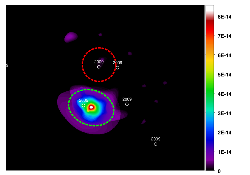
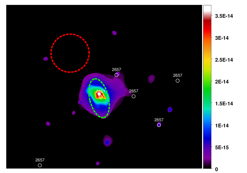
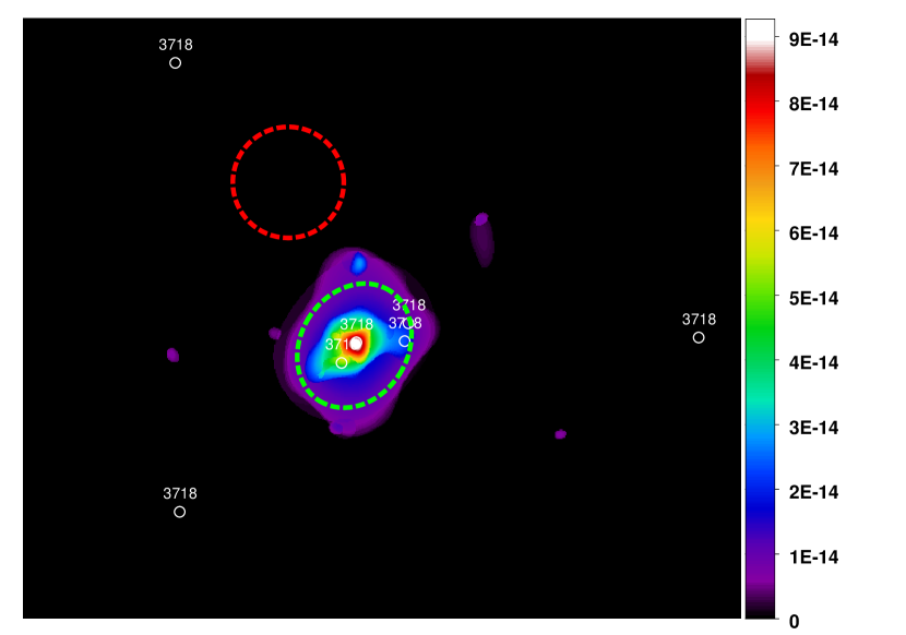
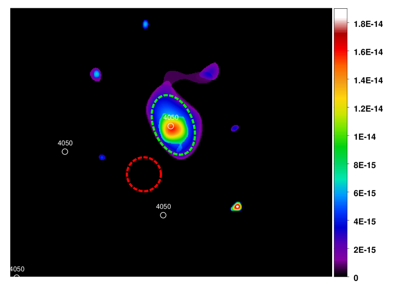
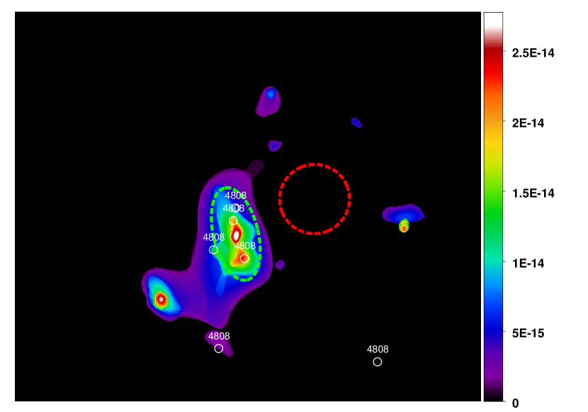
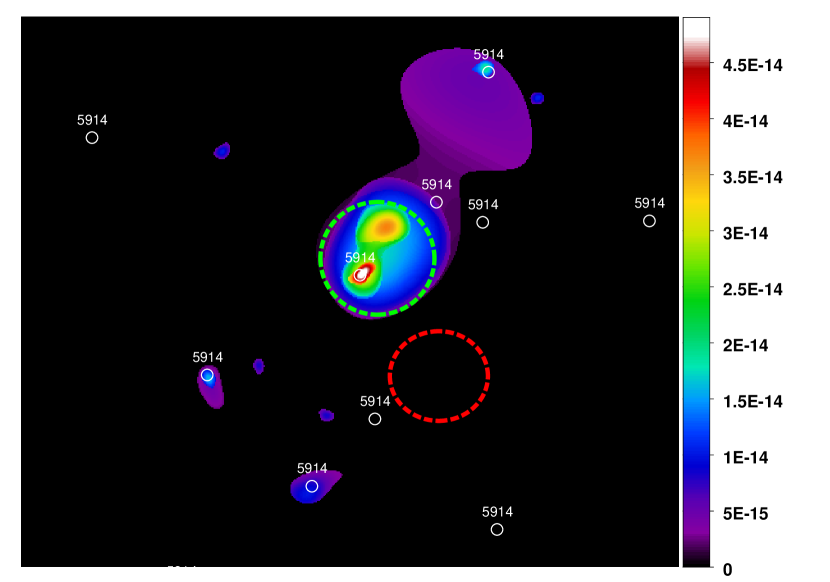
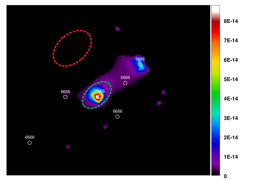
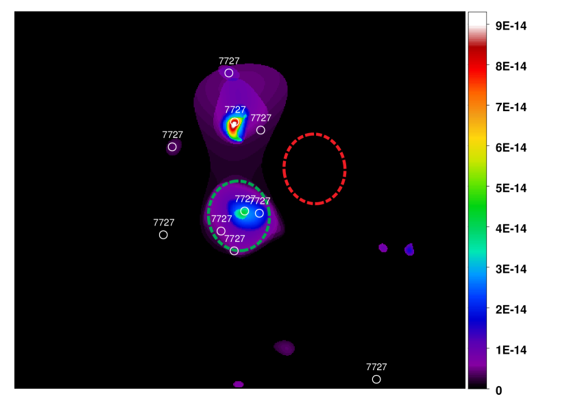
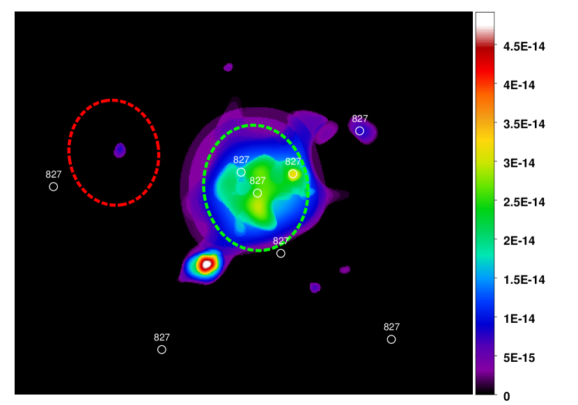
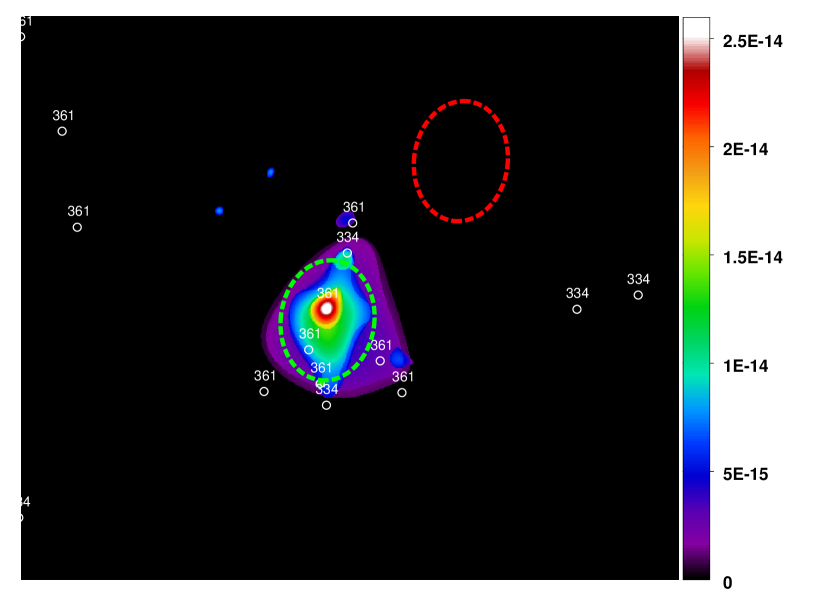
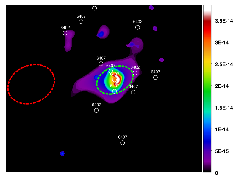
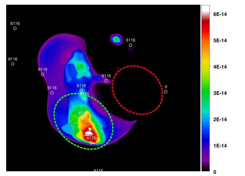
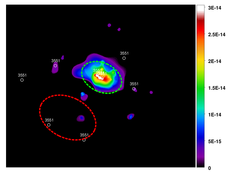
Figure 19: 25 XMM-Newton X-ray pointings for the full sample used in this work. Green dashed ellipses are spectral extraction regions. Red dashed ellipses are background extraction regions. Small white circles represent member galaxies in each group, each denoted with the respective group ID. The color bar scale is counts/s/cm²/arcmin². The original colour bar values were re-scaled in SAOImage DS9 from counts/s/pixel for the XMM-Newton.

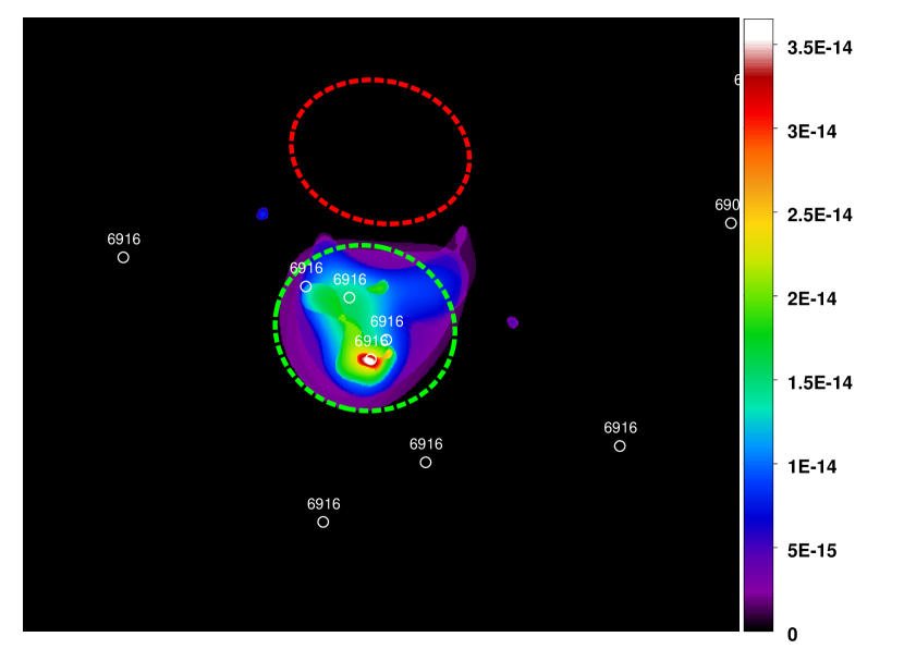
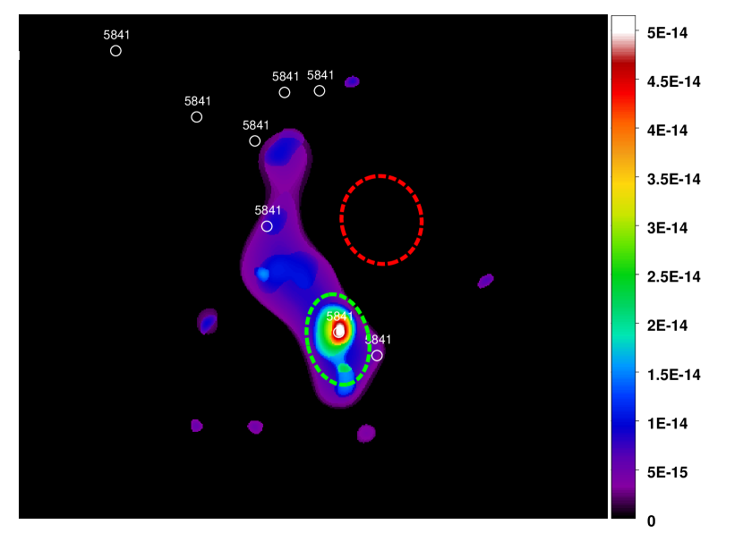
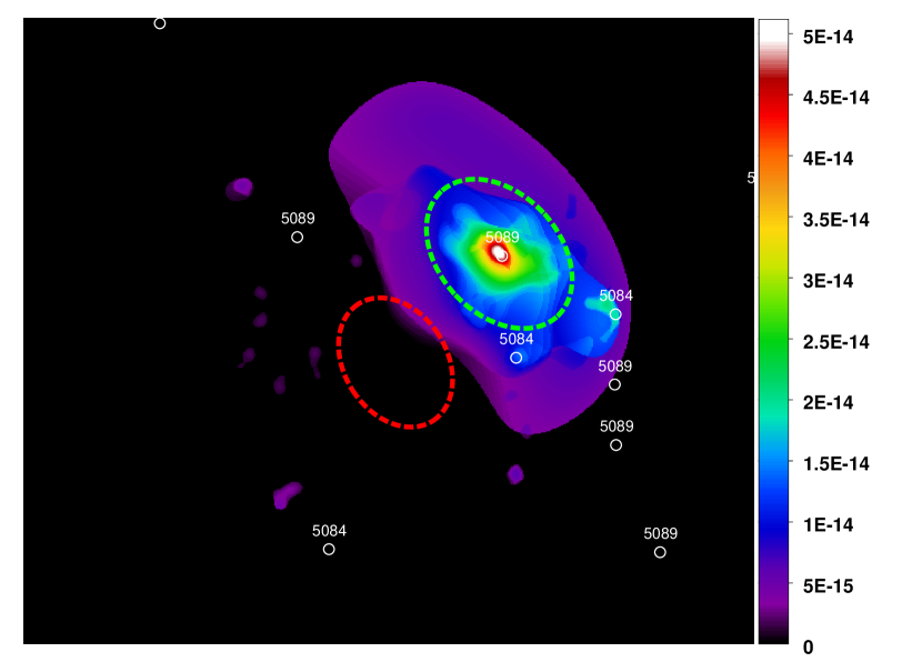
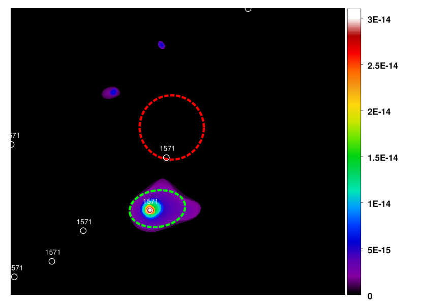
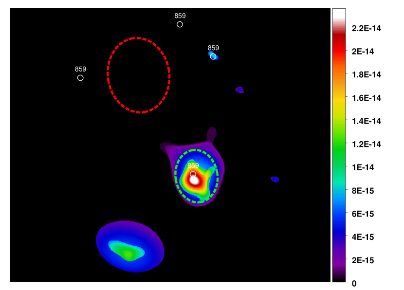
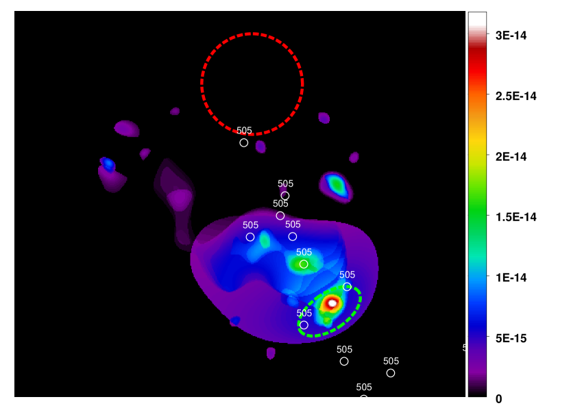
Figure 20: Continued.

Appendix C AXES-2MRS Group Catalogue

In Table7 we describe the X-ray properties of the Full AXES-2MRS Group catalogue. Source flux and luminosities are based on RASS data. The optical properties of the groups are calculated only for groups with at least 5 clean members. The redshifts are reported in the CMB frame, using the catalogues of Tempel et al. (2018). The catalogue is released on CDS.

Table 7: Descriptions of the columns of the AXE-2MRS catalogue. The full VAC is available online at CDS.

Column	Unit	Description	Example
GROUP_ID (1)		2MRS group identification number from Tempel et al. (2018)	2150
AXES_ID (2)		Extended X-ray source ID in the AXES catalog	93280903
RA (3)	deg	X-ray detection right ascension (J2000)	95.56809
DEC (4)	deg	X-ray detection declination (J2000)	–64.67731
NMEM (5)		Number of spectroscopic members in 2MRS group catalogue	23
NMEM_CLEAN (6)		Number of spectroscopic members after the cleaning	23
ZSPEC (7)		2MRS group redshift	0.0281
ZSPEC_CLEAN (8)		Group redshift, assigned using median value of clean members	0.0281
CLUVDISP_GAP (9)	km s-1	Gapper estimate of the cluster velocity dispersion	582.223
GAUSSIANITY (10)		Gaussianity, based on the substructure analysis	G
LX0124 (11)	ergs s-1	Luminosity in the (0.1-2.4) keV band of the cluster, aperture $R_{\text{500c}}$	$2.3\times 10^{43}$
ELX (12)	ergs s-1	Uncertainty on LX0124	$7.59\times 10^{41}$
FLUX052 (13)	ergs s-1 cm-2	Galaxy cluster X-ray flux in the 0.5-2.0 keV band	$7.25\times 10^{-12}$
EFLUX052 (14)	ergs s-1 cm-2	Uncertainty on FLUX052	$2.39\times 10^{-13}$
R_E (15)	arcmin	Apparent radial extent of X-ray emission	16.8