Fast likelihood-free inference in the LSS Stage IV era

Abstract

Forthcoming large-scale structure (LSS) Stage IV surveys will provide us with unprecedented data to probe the nature of dark matter and dark energy. However, analysing these data with conventional Markov Chain Monte Carlo (MCMC) methods will be challenging, due to the increase in the number of nuisance parameters and the presence of intractable likelihoods. In light of this, we present the first application of Marginal Neural Ratio Estimation (MNRE) (a recent approach in simulation-based inference) to LSS photometric probes: weak lensing, galaxy clustering and the cross-correlation power spectra. In order to analyse the hundreds of spectra simultaneously, we find that a pre-compression of data using principal component analysis, as well as parameter-specific data summaries lead to highly accurate results. Using expected Stage IV experimental noise, we are able to recover the posterior distribution for the cosmological parameters with a speedup factor of $\sim 40-60$ compared to classical MCMC methods. To illustrate that the performance of MNRE is not impeded when posteriors are highly non-Gaussian, we test a scenario of two-body decaying dark matter, finding that Stage IV surveys can improve current bounds on the model by up to one order of magnitude. This result supports that MNRE is a powerful framework to constrain the standard cosmological model and its extensions with next-generation LSS surveys.

1 Introduction

Over the last decades cosmology has transitioned to a precision science: a concordance cosmological model has been established, and its parameters have been measured with exquisite precision [1]. This standard cosmological model - also known as $\Lambda$CDM - assumes that the universe is composed of around 5% ordinary matter, 25% cold dark matter (CDM) and 70% dark energy in the form of a cosmological constant $\Lambda$. However, the true nature of its main constituents, dark matter and dark energy, still remains elusive. In addition, several observational discrepancies or unresolved questions are starting to accumulate, like the Hubble tension, $S_{8}$ tension, small-scale CDM crisis, etc (see e.g. [2] for a recent review). For these reasons, in recent years there has been a growing interest in exploring different extensions of the $\Lambda$CDM model, which could shed some light on the mysterious dark components, and possibly offer an explanation for the aforementioned discrepancies.

Forthcoming LSS Stage IV surveys such as ESA’s Euclid satellite mission [3, 4] and the Vera C. Rubin Observatory’s Legacy Survey of Space and Time (VRO/LSST) [5, 6], are aiming to probe the nature of dark matter and dark energy with unprecedented precision. Nevertheless, the vast data volumes to be delivered by these surveys, as well as the ever-expanding space of theories, motivate a re-thinking of the statistical tools used for parameter inference. Part of the difficulty stems from the fact that classical Bayesian inference methods, such as Markov chain Monte Carlo (MCMC), rely on evaluating the likelihood of the data given the model parameters. Often the likelihood function is only tractable at the level of low-order summary statistics, such as the angular power spectra of weak lensing (WL) and galaxy clustering (GC). Even at the power spectra level, theoretical predictions typically require the output of a Boltzmann solver (like CLASS [7, 8] or CAMB [9, 10]) together with some recipe to model non-linear scales, which is computationally expensive. Another problem of likelihood-based methods is that they require sampling the full joint posterior, which means that the time needed to converge increases dramatically with the dimensionality of the parameter space. This is specially troublesome for extended cosmological models, or in situations where the number of nuisance parameters is very large. For instance, for current galaxy surveys such as the Dark Energy Survey (DES) [11], the number of free parameters in a typical analysis is of order $\sim 30$ [12], and this is expected to increase for upcoming surveys such as Euclid and VRO/LSST reaching $\sim 50-100$, which means that a typical MCMC can take up to several weeks.

A first attempt to overcome these obstacles is to use trained emulators, which allow for ultra-fast likelihood evaluations by efficiently interpolating between a small number of simulated cosmological observables [13, 14, 15, 16, 17, 18]. However, these emulators are usually validated on low-order summary statistics (containing only a fraction of the data’s information content), and need to be re-trained every time a new cosmological model is explored. Furthermore, most investigations relying on emulators directly target the observables, quantities that are also dependent on survey specifications, thus making the emulators survey dependent.

Alternatively, novel approaches in simulation-based inference (SBI) allow to perform fast parameter inference without explicitly calculating the likelihood function (see [19] for a recent review). Instead of a likelihood, the key input in SBI is a stochastic simulator that maps from model parameters to realizations of the data; this can be seen as sampling an (implicit) likelihood. The field of SBI has recently seen an impressive rate of progress thanks to deep learning methods, and has found application in different astrophysical contexts [20, 21, 22, 23, 24]. There are multiple methods for SBI, such as Approximate Bayesian Computation (ABC) [25, 26], Neural Likelihood Estimation (NLE) [27], Neural Posterior Estimation (NPE) [28, 29] and Neural Ratio Estimation (NRE) [30, 31]. While both NPE and NLE require an estimation of the normalized probability density [32, 33], NRE turns inference into a simple binary classification task, thus allowing much more flexibility in its network architecture.

In this work, we consider a variant of NRE called Marginal Neural Ratio Estimation (MNRE), implemented via the open-source code Swyft [34]. MNRE uses the output of a simulator to train neural networks that directly learn marginal posterior-to-prior ratios. Since MNRE directly achieves 1- and 2-dimensional marginal posteriors, without needing to sample the full joint posterior, it can be significantly more efficient than traditional likelihood-based methods (as well as other SBI techniques) [35]. Additionally, MNRE offers the flexibility to ignore large numbers of nuisance parameters, targeting only the parameters of interest. MNRE has already been applied to a large variety of problems in astrophysics and cosmology, like analyses of the CMB [35] and 21-cm signal [36], type Ia supernovae [37, 38], strong lensing images [39, 40], point source searches [41], stellar streams [42] or gravitational waves [43, 44, 45].

We show the application of MNRE to accelerate parameter inference from upcoming Stage IV photometric galaxy surveys, such as Euclid or LSST. While other works have applied different SBI methods to optimize the inference from weak lensing probes [46, 47, 48, 49, 50] as well as galaxy clustering probes [51, 52, 53, 54, 55, 56], our work is the first to use SBI to jointly analyze the hundreds of cosmic shear and galaxy clustering spectra that will be measured by Stage IV surveys. Furthermore, we show that MNRE enables a significant reduction in computational time by doing a explicit comparison with MCMC, and derive novel forecast on a non-standard scenario of two-body decaying dark matter.

The paper is structured as follows. In Sec. 2 we discuss the different inference approaches we use in this work, and provide a brief summary of the implementation of MNRE using Swyft. In Sec. 3 we describe the LSS observables that can be constructed from photometric surveys, namely weak lensing and photometric galaxy clustering, detailing our calculation of their angular power spectra in Sec. 3.1 and our approach to obtain synthetic data in Sec. 3.2. Our results are presented in Sec. 4. We first describe our inference setup for Swyft and MCMC in Sec. 4.1, and present the forecast posteriors for the $\Lambda$CDM model in Sec. 4.2 and for the decaying dark matter scenario in Sec. 4.3. We conclude in Sec. 5.

2 Inference methodology

The main goal of most cosmological analyses is to obtain constraints on the parameters of the model under investigation, through a comparison of the theoretical predictions for some observable, given by the model, with observational data. To achieve this, a common approach is to reconstruct the full probability distribution of the parameters ${\bm{\theta}}$ of a chosen cosmological model $\mathcal{M}$ given the observed data ${\bm{x}}$, which we denote as $p({\bm{\theta}}|{\bm{x}})$. Using the Bayes’ theorem, this probability can be expressed as

$$p({\bm{\theta}}|{\bm{x}})=\frac{p({\bm{x}}|{\bm{\theta}})p({\bm{\theta}})}{p({\bm{x}})}.$$ (2.1)

where $p({\bm{x}}|{\bm{\theta}})$ is called likelihood, $p({\bm{\theta}})$ is the prior, $p({\bm{x}})$ is the evidence, and $p({\bm{\theta}}|{\bm{x}})$ is known as posterior. The main goal of such an approach is therefore to sample the posterior distribution $p({\bm{\theta}}|{\bm{x}})$, as having this probability allows to find the best estimates for the parameters, their marginalised confidence levels and the degeneracies between them. However, there is not a unique approach to sample the posterior probability distribution; one could exploit methods known as Monte-Carlo Markov Chain (MCMC), where the parameter space is explored randomly (Monte-Carlo) with each step being dependent only on the previous state (Markov process). This approach can be implemented through different algorithms, such as Metropolis-Hastings [57], Nested Sampling [58], ensemble sampling [59], etc. Notice that while the MCMC approach is commonly associated only with the Metropolis-Hastings algorithm, all traditional likelihood-based methods follow the same principles making them part of the MCMC class.

Nevertheless, we must stress that obtaining the full posterior distribution $p({\bm{\theta}}|{\bm{x}})$ is not the real goal of most cosmological analysis. If we are interested in a subset of parameters ${\bm{\vartheta}}\subset{\bm{\theta}}$, what we actually need are the marginalised distribution for each parameter $p(\vartheta_{i}|{\bm{x}})$ in order to obtain confidence level interval on each $\vartheta_{i}$ separately, or, at most, the marginalised distribution for two parameters $\vartheta_{i}$ and $\vartheta_{j}$ in order to visualise their correlations. For such a reason it beneficial to consider methods returning directly the marginal posteriors.

In this work we will follow this latter approach, focusing on a recent algorithm in SBI called Marginal Neural Ratio Estimation (MNRE), and we will compare its performance with that of MCMC. In the rest of this section, we provide more details on the Metropolis-Hastings and MNRE algorithms. We also give a brief summary of the Fisher matrix formalism, since we use this to define our prior boundaries in Sec. 4.1.

2.1 Fisher matrix

In order to explore the posterior distribution, most sampling method require at least an approximate knowledge of the possible values the parameters can take, as well as an initial estimate of the correlation between them. This information can in principle be provided by the results of previous experiments. Here, however, we decide to obtain such information independently, by exploiting the Fisher matrix approach [60, 61]. This approach provides a reconstruction of the posterior distribution which relies on assuming that this is Gaussian. The Fisher matrix is defined as the Hessian of the likelihood function and, within the assumption of a Gaussian posterior, coincides with the inverse of the parameters covariance matrix. For two generic parameters $\theta_{\alpha}$ and $\theta_{\beta}$, the element of the Fisher matrix $F_{\alpha\beta}$ is defined as

$$F_{\alpha\beta}=-\left.\frac{\partial^{2}\mathrm{ln}\mathcal{L}}{\partial\theta_{\alpha}\partial\theta_{\beta}}\right\rvert_{{\bm{\theta}}^{0}}\,,$$ (2.2)

where ${\bm{\theta}}^{0}$ is the peak of the likelihood distribution $\mathcal{L}=p({\bm{x}}|{\bm{\theta}})$, which in the case of forecasts coincides with the assumed fiducial cosmology. In the following, we will focus on the LSS observables that can be obtatined by photometric surveys, namely weak lensing and galaxy clustering, that we will express in terms of the angular power spectra $C_{ij}^{AB}(\ell)$, where $A$ and $B$ run over the galaxy and lensing fields, while $i$ and $j$ run over the possible combination of the tomographic redshift bins of the survey. It can be shown that, for such observables, the Fisher matrix can be expressed as [4]

$$F_{\alpha\beta}=\sum_{\ell=2}^{\ell_{\mathrm{max}}}\sum_{AB,A^{\prime}B^{\prime}}\sum_{ijmn}\frac{\partial C^{AB}_{ij}(\ell)}{\partial\theta_{\alpha}}\mathbf{C}^{-1}\left[C_{ij}^{AB}(\ell),C_{mn}^{A^{\prime}B^{\prime}}(\ell)\right]\frac{\partial C^{A^{\prime}B^{\prime}}_{mn}(\ell)}{\partial\theta_{\beta}}\,$$ (2.3)

where $\mathbf{C}$ is the data covariance matrix. We give more details on how we model this quantity and the observable power spectra in Sec. 3.

2.2 Likelihood-based inference with Metropolis-Hastings

The general principle of traditional likelihood-based methods is to generate samples of the full joint posterior distribution $p({\bm{\theta}}|{\bm{x}})$, and then marginalize to get the 1- and 2-dimensional posteriors of interest. With MCMC, this is achieved by starting from a certain point in parameter space ${\bm{\theta}}^{t}$ and selecting the next one ${\bm{\theta}}^{(t+1)}$ according to a given proposal distribution $g({\bm{\theta}}^{(t+1)},{\bm{\theta}}^{t})$. In the Metropolis-Hastings (MH) algorithm, this new sample is “accepted” with probability

$$p=\mathrm{min}\left\{1,\frac{p({\bm{\theta}}^{(t+1)}|{\bm{x}})}{p({\bm{\theta}}^{t}|{\bm{x}})}\right\}.$$ (2.4)

We then repeat the cycle, drawing a new proposal based on the last element in the chain. Therefore, the MH algorithm does not only accept new points with higher likelihood, but also points with smaller likelihood at a smaller rate, so that it can explore the parameter space and trace the underlying posterior distribution. In this way, we end generating the weights of each point in parameter space, i.e. the number of times we waited and did not move. If the number of steps in the chain is big enough, then these weights are proportional to the posterior $p({\bm{\theta}}|{\bm{x}})$. Notice that to exploit the MH algorithm we also need to tune several parameters, such as the starting point of the chains, the prior range for the parameters and the starting proposal, with the choice for these settings significantly affecting the performances of the method [62].

In Sec. 4 and Appendix C, we will present cosmological results obtained through the Metropolis-Hastings algorithm as it is implemented in the publicly available Bayesian analysis software for cosmology, MontePython [63] and Cobaya [64].

2.3 Simulation-based inference with MNRE

In simulation-based inference (SBI), the information about the likelihood $p({\bm{x}}|{\bm{\theta}})$ is implicitly accessed via a stochastic simulator, mapping from model parameters ${\bm{\theta}}$ to data realizations ${\bm{x}}$. By drawing parameters from the prior $p({\bm{\theta}})$ and calling the simulator, we can generate $N$ data-parameter pairs $\{({\bm{x}}^{1},{\bm{\theta}}^{1}),...,({\bm{x}}^{N},{\bm{\theta}}^{N})\}$ drawn from the joint distribution $p({\bm{x}},{\bm{\theta}})=p({\bm{x}}|{\bm{\theta}})p({\bm{\theta}})$. Then we can also construct samples from the product of marginal probabilities $p({\bm{x}})p({\bm{\theta}})$ by randomly shuffling the pair components. The strategy of Neural Ratio Estimation (NRE) is to use these two different sets of data-parameter pairs to train a neural network to approximate the following ratio:

$$r({\bm{x}};{\bm{\theta}})\equiv\frac{p({\bm{x}},{\bm{\theta}})}{p({\bm{x}})p({\bm{\theta}})}=\frac{p({\bm{x}}|{\bm{\theta}})}{p({\bm{x}})}=\frac{p({\bm{\theta}}|{\bm{x}})}{p({\bm{\theta}})},$$ (2.5)

where the second and third equality follow trivially from Bayes’ theorem in Eq. 2.1. In other words, determining $r({\bm{x}};{\bm{\theta}})$ is equivalent to determining the likelihood-to-evidence ratio or the posterior-to-prior ratio. This will ultimately allow us to obtain posterior samples by drawing samples from the prior $p({\bm{\theta}})$ and weighting them by $r({\bm{x}};{\bm{\theta}})$. To compute $r({\bm{x}};{\bm{\theta}})$, we optimise a binary classifier $d_{\phi}({\bm{x}},{\bm{\theta}})$ (with $\phi$ denoting the set of learnable parameters) to distinguish between jointly drawn and marginally drawn pairs, i.e. it should be trained such that

$$d_{\phi}({\bm{x}},{\bm{\theta}})\simeq\begin{cases}1\ \ \mathrm{if}\ \ ({\bm{x}},{\bm{\theta}})\sim p({\bm{x}},{\bm{\theta}}),\\ 0\ \ \mathrm{if}\ \ ({\bm{x}},{\bm{\theta}})\sim p({\bm{x}})p({\bm{\theta}}).\end{cases}$$ (2.6)

This learning problem is associated to the minimization of the following loss function

$$\ell[d_{\phi}({\bm{x}},{\bm{\theta}})]=-\int d{\bm{x}}d{\bm{\theta}}\left[p({\bm{x}},{\bm{\theta}})\ln d_{\phi}({\bm{x}},{\bm{\theta}})+p({\bm{x}})p({\bm{\theta}})\ln(1-d_{\phi}({\bm{x}},{\bm{\theta}}))\right],$$ (2.7)

also known as binary cross-entropy. Indeed, by analytically minimizing the above functional $\ell[d_{\phi}({\bm{x}},\theta)]$ one can show that this yields $d^{\star}_{\phi}({\bm{x}},{\bm{\theta}})=\sigma(\ln r({\bm{x}},{\bm{\theta}}))$, where $\sigma(x)=[1+\mathrm{exp}(-x)]^{-1}$ denotes the sigmoid function. In practice, to find the optimal parameters $\phi$ of the network we minimize a sample-based approximation of the loss function in Eq. 2.7 using stochastic gradient descent.

This method allows to directly estimate marginal posteriors by omitting parameters from network’s input, a variant called Marginal Neural Ratio Estimation (MNRE) . More precisely, if ${\bm{\vartheta}}$ denote the parameters of interest, which are usually a low-dimensional subset of the full parameter set ${\bm{\vartheta}}\subset{\bm{\theta}}=({\bm{\vartheta}},{\bm{\eta}})$, we can directly estimate $r({\bm{x}};{\bm{\vartheta}})=p({\bm{\vartheta}}|{\bm{x}})/p({\bm{\vartheta}})$. In practice, we will only be interested in obtaining 1- and 2-dimensional marginal posteriors, i.e. ${\bm{\vartheta}}=\theta_{k}$ for some $k$ or ${\bm{\vartheta}}=(\theta_{i},\theta_{j})$ for some $(i,j)$. For more details about the algorithm, we refer the reader to [35] and [34].

3 Large-Scale Structure observables and synthetic data

The main purpose of this work is to compare the performances of different analysis pipelines in inferring constraints on cosmological parameters from upcoming LSS observations. One of the fundamental ingredients to achieve this goal is the possibility to simulate the observational data we expect to obtain from such surveys. In this section, we provide details on our modelling of a particular set of LSS observables, the assumptions we do to obtain theoretical predictions, and the calculation of the observational noise that we use to obtain synthetic data for LSS surveys.

3.1 Theoretical Predictions

For this work, we focus on the main observables that can be obtained from a photometric galaxy survey, namely weak lensing (WL), i.e. the correlation between shear in the galaxy shapes, and galaxy clustering (GCph), i.e. the correlation between galaxy positions. Together with these, we also consider the cross-correlation of the two observables (XC), and we will refer to the full combination as the 3x2pt statistics.

We choose to obtain theoretical predictions on these correlations by modelling their angular power spectra in multipole space, and dividing our observations in redshift bins in order to exploit the tomographic information. These angular power spectra can be obtained, applying the Limber approximation [65], as

$$C^{AB}_{ij}(\ell)=\int{\frac{{\rm d}z}{H(z)r^{2}(z)}W_{i}^{A}(z)W_{j}^{B}(z)P_{AB}(k_{\ell}(z),z)}\,$$ (3.1)

where the indices $A,B$ run over the two observables (GCph and WL) that we denote respectively with ${\rm g}$ and $\epsilon$, the indices $i,j=1,...,N_{\mathrm{bin},z}$ run over redshift bins, $H(z)$ is the Hubble parameter, $r(z)$ the comoving distance, $W_{i}^{A}(z)$ is the kernel function of the considered observable, $P_{AB}(k,z)$ is the power spectrum corresponding to the considered observable combination and $k_{\ell}(z)=(\ell+1/2)/r(z)$.

The GC term is modelled through the kernel $W_{i}^{\rm g}(z)$ and the power spectrum $P_{\rm gg}$

$$W_{i}^{\rm g}(z) =n_{i}^{\rm g}(z)H(z)\,,$$ (3.2)

$$P_{\rm gg}(k,z) =b_{\rm g}^{2}(z)P_{\delta\delta}(k,z)\,,$$ (3.3)

where $n_{i}^{\rm g}(z)$ is the normalized distribution in redshift of the observed galaxies in the $i$-th redshift bin, $P_{\delta\delta}(k,z)$ is the matter power spectrum and $b_{\rm g}(z)$ is the galaxy bias, which accounts for the fact that we are observing galaxies, i.e. a biased tracer of the total matter distribution. In order to account for uncertainties in galaxy formation and its relation to the underlying distribution of matter, we do not attempt to model the galaxy bias, but rather treat it as a free nuisance parameter $b_{i}$ assumed to be constant in each redshift bin.

The WL term is instead able to trace directly the total matter distribution, as the observable is the shear of galaxy shapes due to the lensing effect caused by the matter distribution between the observer and the galaxies. However, this observable is also affected by astrophysical systematics. As the shear is obtained by observing galaxy ellipticities, we need to account for effects that can introduce correlations that are not of cosmological origin. Such an effect is usually referred to as Intrinsic Alignment (IA) [66, 67, 68]. We include this effect by defining the WL angular power spectra as [4]

$$C_{ij}^{\epsilon\epsilon}(\ell)=C_{ij}^{\gamma\gamma}(\ell)+C_{ij}^{{\rm I}\gamma}(\ell)+C_{ij}^{\rm II}(\ell),$$ (3.4)

where $\gamma$ refers to the cosmological shear field and $I$ are the contributions due to IA. The terms entering Eq. 3.4 can be obtained through Eq. 3.1, modelling the shear and IA kernels as [4]

$$W_{i}^{\gamma}(z) =\frac{3}{2}H^{2}_{0}\Omega_{{\rm m}}(1+z)r(z)\int_{z}^{z_{\rm max}}{{\rm d}z^{\prime}n_{i}^{\gamma}(z^{\prime})\left[\frac{r(z^{\prime})-r(z)}{r(z^{\prime})}\right]}\,,$$ (3.5)

$$W_{i}^{\rm I}(z) =n_{i}^{\gamma}(z)H(z)\,,$$ (3.6)

where $H_{0}$ is the Hubble constant, $\Omega_{\rm m}$ the present day matter abundance of the Universe, and $n_{i}^{\gamma}(z)$ is the normalized distribution in the $i$-th redshift bin for the galaxies used to measure the shear effect. The power spectra entering these terms can be modelled as

$$P_{\gamma\gamma}(k,z) =P_{\delta\delta}(k,z)\,,$$ (3.7)

$$P_{\rm II}(k,z) =f_{\rm IA}^{2}(z)P_{\delta\delta}(k,z)\,,$$ (3.8)

where the first equation shows that shear is an unbiased tracer of the total matter distribution, and the second equation includes the $f_{\rm IA}(z)$ term modelling IA contribution. For this term, we exploit the redshift-dependent non-linear alignment (zNLA) model [66, 67, 68], which allows to define [4]

$$f_{\rm IA}(z)=-{A}_{\rm IA}\mathcal{C}_{\rm IA}\frac{\Omega_{\rm m}}{D(z)}(1+z)^{\eta^{\rm IA}}\,,$$ (3.9)

where $A_{\rm IA}$ and $\eta_{\rm IA}$ are the free parameters of the IA model, $\mathcal{C}_{\rm IA}=0.0134$ and $D(z)$ is the growth factor of matter perturbations. With these equations in hand, we are now able to obtain theoretical predictions for our observables as

$$C_{ij}^{\epsilon\epsilon}(\ell)= \int{\frac{{\rm d}z}{H(z)r^{2}(z)}\left[W_{i}^{\gamma}(z)W_{j}^{\gamma}(z)P_{\gamma\gamma}(k_{\ell}(z),z)+W_{i}^{\rm I}(z)W_{j}^{\gamma}(z)P_{\rm I\gamma}(k_{\ell}(z),z)\right.}$$

$$+\left.W_{i}^{\rm I}(z)W_{j}^{\rm I}(z)P_{\rm II}(k_{\ell}(z),z)\right]\,,$$ (3.10)

$$C_{ij}^{\rm gg}(\ell)= \int{\frac{{\rm d}z}{H(z)r^{2}(z)}W_{i}^{\rm g}(z)W_{j}^{\rm g}(z)P_{\rm gg}(k_{\ell}(z),z)}\,,$$ (3.11)

$$C_{ij}^{\rm g\epsilon}(\ell)= \int\frac{{\rm d}z}{H(z)r^{2}(z)}\left[W_{i}^{\rm g}(z)W_{j}^{\gamma}(z)P_{\rm g\gamma}(k_{\ell}(z),z)+W_{i}^{\rm g}(z)W_{j}^{\rm I}(z)P_{\rm gI}(k_{\ell}(z),z)\right],$$ (3.12)

with the mixed power spectra being

$$P_{\rm g\gamma}(k,z) =b_{\rm g}(z)P_{\delta\delta}(k,z)\,,$$ (3.13)

$$P_{\rm gI}(k,z) =b_{\rm g}(z)f_{\rm IA}(z)P_{\delta\delta}(k,z)\,,$$ (3.14)

$$P_{\rm I\gamma}(k,z) =f_{\rm IA}(z)P_{\delta\delta}(k,z)\,.$$ (3.15)

The only ingredients left to be able to compute the $C_{ij}^{AB}(\ell)$ are the cosmological functions entering the expressions, i.e. the Hubble parameter $H(z)$, the comoving distance $r(z)$ and the matter power spectrum $P_{\delta\delta}(k,z)$. Given a set of cosmological parameters, we obtain these from the public Boltzmann solvers CLASS [7, 8] and CAMB [9, 10].

3.2 Synthetic data and fiducial model

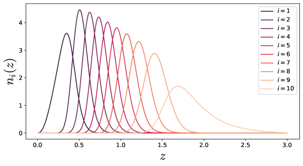
Figure 1: Galaxy redshift distribution $n(z)$ obtained by convolving with the photometric redshift uncertainties using Eq. 3.17. The figure shows $N_{\mathrm{bin},z}=10$ different tomographic redshift bins delimited by redshift values specified in Eq. 3.19.

Once we obtain the theoretical predictions for the observable power spectra, we can use these to simulate synthetic datasets as they would be obtained from an upcoming LSS survey. In order to do so, we can compute predictions for a given fiducial cosmological model that we assume to be the one describing the Universe. The spectra obtained in this way will play the role of observed data, on top of which we can add an observational noise that accounts for the design and specifications of the survey we want to consider.

In this work, we take the flat $\Lambda$CDM model as our fiducial scenario. With this assumption, the parameters we need to choose to obtain the cosmological quantities from the Boltzmann solvers are the baryon and cold dark matter abundances ($\omega_{i}=\Omega_{i}h^{2}$ for $i=\mathrm{b},\mathrm{cdm}$), the Hubble constant ($H_{0}$) and the amplitude and tilt of the primordial power spectrum of density fluctuations ($A_{\rm s}$ and $n_{\rm s}$) . We report our choice for the fiducial values for these parameters in Tab. 1.

Parameter	Fiducial
$H_{0}$ [km s-1 Mpc-1]	67.0
$100~{}\omega_{\rm b}$	2.2445
$\omega_{\rm cdm}$	0.1206
$n_{\rm s}$	0.96
$\ln{(10^{10}A_{\rm s})}$	3.0569
$A_{\rm IA}$	1.72
$\eta_{\rm IA}$	-0.41
$b_{i}$	$\sqrt{1+\bar{z}_{i}}$

Table 1: Fiducial cosmological and nuisance parameter values used to generate the synthetic dataset.

Furthermore, one key ingredient needed to obtain the $C^{AB}_{ij}(\ell)$ are the binned galaxy distributions $n_{i}^{\rm g}(z)$ and $n_{i}^{\gamma}(z)$. For the sake of simplicity, we assume here that the two distributions coincide and we model the unbinned distribution as

$$n(z)\propto\left(\frac{z}{z_{0}}\right)^{2}\exp{\left[-\left(\frac{z}{z_{0}}\right)^{\frac{3}{2}}\right]}\,,$$ (3.16)

with $z_{0}=z_{m}/\sqrt{2}$, where $z_{m}$, the median redshift of the survey, is reported in Tab. 2. From this, we can obtain the binned distribution, by convolving $n(z)$ with the photometric redshift distribution $p_{\rm ph}(z_{p}|z)$, i.e. the probability of measuring a redshift $z_{p}$ given a true redshift $z$

$$n_{i}(z)=\frac{\int_{z_{\rm min}}^{z_{\rm max}}{{\rm d}z_{p}n(z)p_{\rm ph}(z_{p}|z)}}{\int_{z_{\rm min}}^{z_{\rm max}}{{\rm d}z\int_{z_{-}}^{z_{+}}{{\rm d}z_{p}n(z)p_{\rm ph}(z_{p}|z)}}}\,,$$ (3.17)

where $z_{\rm min}$ and $z_{\rm max}$ are the limiting redshift of the survey. $z_{-}$ and $z_{+}$ are the limiting redshift of the $i$-th bin, and we model $p_{\rm ph}(z_{p}|z)$ as [4]

$$p_{\rm ph}(z_{p}|z)= \frac{1-f_{\rm out}}{\sqrt{2\pi}\sigma_{b}(1+z)}\exp{\left\{-\frac{1}{2}\left[\frac{z-c_{b}z_{p}-z_{b}}{\sigma_{b}(1+z)}\right]^{2}\right\}}$$

$$+\frac{f_{\rm out}}{\sqrt{2\pi}\sigma_{o}(1+z)}\exp{\left\{-\frac{1}{2}\left[\frac{z-c_{o}z_{p}-z_{o}}{\sigma_{o}(1+z)}\right]^{2}\right\}}\,,$$ (3.18)

where the set of parameters describing the uncertainties in redshift are shown in Tab. 2. We divide the redshift range of the survey in $N_{\mathrm{bin},z}=10$ equi-populated bins, i.e. bins in redshift containing the same number of galaxies, obtained by computing the integral in Eq. 3.17. The set of redshifts delimiting the 10 bins is

$$\vec{z}_{\rm lim}=\{0.001,0.417,0.5593,0.677,0.787,0.899,1.017,1.153,1.322,1.573,3.\}\,$$ (3.19)

and we show the resulting galaxy redshift distribution $n_{i}$ in Fig. 1. In addition to the cosmological parameters, we also need to set the fiducial values of the parameters describing the modelling of systematic effects. As indicated in Tab. 1, for the 10 galaxy bias $b_{i}$ we take $\sqrt{1+\bar{z}_{i}}$, where $\bar{z}_{i}$ are the mean redshifts of each bin, while for the IA parameters we choose values compatible with the literature [4]. All these ingredients allow to compute the fiducial angular spectra for the 3x2pt combination of observables, shown in Fig. 2.

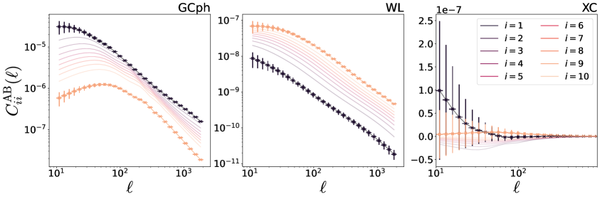
Figure 2: Angular power spectrum $C^{\rm AB}_{ii}(\ell)$ for the photometric LSS probes (3x2pt). From left to right: photometric galaxy clustering (GCph), weak lensing (WL) and the cross-correlation (XC). For simplicity, we only show the auto-correlation for the 10 tomographic redshift bins corresponding to Fig. 1. For the redshift bins $n_{1}$ and $n_{10}$, we also show the observational errors computed following the discussion in Sec. 3.2.1.

3.2.1 Noise and covariance calculation

As we are creating synthetic data that will mimic what we can obtain from observations, a key ingredient to be modelled is the observational uncertainty affecting the measurements, and how this propagates to the angular spectra that we compare with theoretical predictions. For simplicity, we assume that our final measured spectra $C_{ij}^{AB}(\ell)$ are distributed following a multivariate Gaussian distribution, with a covariance matrix $\mathbf{C}\left[C_{ij}^{AB}(\ell),C_{mn}^{A^{\prime}B^{\prime}}(\ell^{\prime})\right]$ that we model as [4, 69]

$$\mathbf{C}\left[C_{ij}^{AB}(\ell),C_{mn}^{A^{\prime}B^{\prime}}(\ell^{\prime})\right]= \frac{\delta^{\rm K}_{\ell\ell^{\prime}}}{(2\ell+1)f_{\rm sky}\Delta\ell}\left\{\left[C_{im}^{AA^{\prime}}(\ell)+N_{im}^{AA^{\prime}}(\ell)\right]\left[C_{jn}^{BB^{\prime}}(\ell^{\prime})+N_{jn}^{BB^{\prime}}(\ell^{\prime})\right]+\right.$$

$$\left.\left[C_{in}^{AB^{\prime}}(\ell)+N_{in}^{AB^{\prime}}(\ell)\right]\left[C_{jm}^{BA^{\prime}}(\ell^{\prime})+N_{jm}^{BA^{\prime}}(\ell^{\prime})\right]\right\}\,,$$ (3.20)

where $\delta^{\rm K}_{\ell\ell^{\prime}}$ is the Kronecker delta function, $f_{\rm sky}$ is the fraction of sky observed by our simulated survey, $\Delta\ell$ the width of the bin in $\ell$ we divide our observations into, and the $A,B$ indexes run over the observables (${\rm g}$, $\epsilon$), while the $(i,j,m,n)$ run over the redshift bins. The information on the observational uncertainties is encoded in the noise terms $N_{ij}^{AB}(\ell)$; we assume this noise to be uncorrelated between different redshift bins and observables and therefore model it as

$$N_{ij}^{AB}(\ell)=\quad\begin{cases}\delta^{\rm K}_{ij}/\bar{n}_{\rm g}^{i}\ \ \ &A=B={\rm g}\,,\\ \delta^{\rm K}_{ij}\sigma_{\epsilon}^{2}/\bar{n}_{\rm g}^{i}\ \ &A=B=\epsilon\,,\\ 0\ \ \ &A\neq B\,,\end{cases}\quad$$ (3.21)

where $\bar{n}_{\rm g}^{i}$ is the number of observed galaxies over the survey area in the $i$-th redshift bin and $\sigma_{\epsilon}$ is the intrinsic ellipticity error, i.e. the uncertainty due to the intrinsic shape of the observed galaxies, which is unknown due to our surveys only observing galaxies that have been lensed by the LSS. We show the value used in our synthetic data in Tab. 2. Notice that in the rest of the paper, we will keep the covariance matrix fixed to the value obtained in the fiducial cosmology.

$z_{m}$	$\bar{n}_{\rm g}$ [arcmin-2]	$f_{\rm sky}$	$\Delta\log_{10}\ell$	$\sigma_{\epsilon}$	$f_{\rm out}$	$c_{b}$	$z_{b}$	$\sigma_{b}$	$c_{o}$	$z_{o}$	$\sigma_{o}$
0.9	30	0.35	0.08	0.3	0.1	1.0	0	0.05	1.0	0.1	0.05

Table 2: Parameters describing the survey specifications. All the quantities are defined within Sec. 3.2. Notice that in this table we report the value of $\Delta\log_{10}\ell$ rather than $\Delta\ell$, as we choose to perform our analysis using $N_{\mathrm{bin},\ell}=29$ multipole bins, whose limits are logarithmically spaced between $\ell_{\rm min}=10$ and $\ell_{\rm max}=2000$.

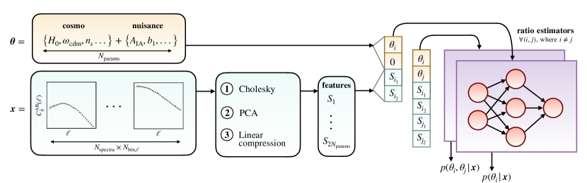
Figure 3: Illustration of the network architecture, mapping from input parameters ${\bm{\theta}}$ and data ${\bm{x}}$ to the 1- and 2-dimensional marginal posteriors of interest. First, the different angular spectra are compressed into features following three steps: i) Cholesky decomposition; ii) Principal Component Analysis; iii) linear compression network. Then, each parameter $\theta_{i}$ is linked with 2 features $(S_{i_{1}},S_{i_{2}})$ and fed as input to the ratio estimators $r({\bm{x}};\theta_{i})$ and $r({\bm{x}};\theta_{i},\theta_{j})$, which are trained with MLPs.

4 Results

4.1 Inference setup

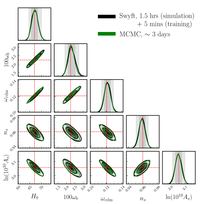
Figure 4: Forecast constraints on the $\Lambda$CDM cosmological parameters from 3x2pt Stage IV photometric probes, using both Swyft (black contours) and MCMC (green contours). The red dashed lines indicate the injected values. Swyft shows an excellent agreement with MCMC at significantly reduced computational cost.

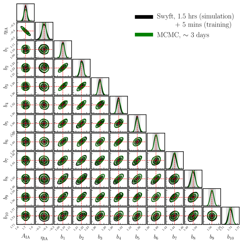
Figure 5: Forecast constraints on the nuisance parameters from 3x2pt Stage IV photometric probes, using both Swyft (black contours) and MCMC (green contours). The red dashed lines indicate the injected values.

To perform the Swyft analysis we need essentially two ingredients: a forward simulator and a neural network design. A simulator with the same statistical content as the multivariate Gaussian likelihood described in Sec. 3.2.1 is defined by the next steps:

1. Given the cosmological and nuisance parameters, compute each angular spectra $C^{AB}_{ij}$ according to Eq. 3.10-Eq. 3.12, with the help of a Boltzmann solver. For the analyses shown in this section, we use the public code CLASS [7, 8] with the halofit prescription [72] for the non-linear corrections to the matter power spectrum.

2. Add a noise realization to each angular spectrum, $\hat{C}^{AB}_{ij}=C^{AB}_{ij}+n^{AB}_{ij}$, where $n^{AB}_{ij}$ is drawn from the multivariate normal distribution $\mathcal{N}(0,\mathbf{C})$, with covariance matrix $\mathbf{C}$ given by Sec. 3.2.1.

We generate $5\times 10^{4}$ simulations by varying all cosmological and nuisance parameters,

$$\left\{H_{0},100\omega_{b},\omega_{\rm cdm},n_{s},\mathrm{ln}(10^{10}A_{s})\right\}+\left\{A_{\rm IA},\eta_{\rm IA},b_{1},...,b_{10}\right\}.$$ (4.1)

Each parameter $\theta_{i}$ is drawn from an uniform prior

$$\theta_{i}\sim\mathcal{U}([\theta^{0}_{i}-5\sigma_{i}^{F},\theta^{0}_{i}+5\sigma_{i}^{F}]),$$ (4.2)

where $\theta^{0}_{i}$ denotes the fiducial value in Tab. 1 and the error $\sigma_{i}^{F}$ is estimated from the Fisher matrix in Eq. 2.3 as $\sigma_{i}^{F}=\sqrt{(F^{-1})_{ii}}$. We have chosen these reasonably narrow priors just for simplicity. However, we remark that wide priors can easily be accommodated in Swyft by using an extension of the algorithm called Truncated Marginal Neural Ratio Estimation (TMNRE) [35], which applies a truncation scheme to quickly zoom into the relevant region of the parameter space. For example, this could be helpful to study prior volume effects arising in LSS analyses [73, 74]. We leave this study to future work.

Regarding the design for the network, we split it into a first part performing data compression, and a second part performing the actual inference (see Fig. 3 for a schematic diagram). More specifically, we found that a pre-compression of data using principal component analysis (PCA), as well as parameter-specific data summaries lead to results with high accuracy and precision. We give more details about the network architecture in Appendix A. We use $80\%$ of the simulations as the training dataset, and the remaining $20\%$ as the validation dataset . We use the Adam optimizer with an initial learning rate of $10^{-3}$ and a batch size of $256$. The learning rate is reduced by a factor of $0.1$ whenever the validation loss plateaus for $3$ epochs, and the training is run for no longer than $40$ epochs. The output of the trained network is the different estimated ratios for the parameters of interest.

On the other hand, we perform the MCMC analysis with the Metropolis-Hastings algorithm by implementing the aforementioned multivariate Gaussian likelihood in the public code MontePython [63]. To allow for a fair comparison, we use the same parameters and priors as for the Swyft analysis (see Eq. 4.2). We launch 18 chains, which we assume to be converged using the Gelman-Rubin criterion $R-1<0.01$ [75]. The chains are post-processed with getdist [76]. In order to accelerate convergence, for the initial proposal distribution we use the parameter covariance matrix estimated from the inverse of the Fisher matrix, $(F^{-1})_{ij}$. Finally, let us remark that for both Swyft and MCMC analyses we consider a noiseless observation, i.e. $\hat{C}^{AB}_{ij}({\bm{\theta}}^{0})=C^{AB}_{ij}({\bm{\theta}}^{0})$ . In Appendix C we compare our MCMC results with those obtained using a different Boltzmann solver (CAMB [9, 10]) and a different MCMC sampler (Cobaya [64]), finding good agreement between the different software tools.

4.2 Forecast posteriors for $\Lambda$CDM

In Fig. 4 we show the marginalized 1- and 2-dimensional posteriors of the cosmological parameters from the mock data analysis of 3x2pt Stage IV photometric probes. These have been obtained using MNRE with the Swyft code (black contours) and MCMC with the Metropolis-Hastings algorithm (green contours). The red dashed lines indicate the true values of the parameters.

We find that the Swyft and MCMC posterior distributions are in excellent agreement, and both yield a correct reconstruction of the fiducial cosmology. Additionally, using 72 CPU cores, the Swyft posteriors were obtained in less than $2$ hours, compared to the $\sim 3$ days required when using MCMC. This corresponds to a speedup factor of $\sim 40$, even after fine-tuning the proposal distribution for the MCMC. The substantial reduction in computing time is explained by two factors. First, MNRE directly estimates the marginal posteriors $p(\theta_{i}|{\bm{x}})$ and $p(\theta_{i},\theta_{j}|{\bm{x}})$, so it requires far fewer simulation runs than first sampling the full (17-dimensional) joint distribution $p({\bm{\theta}}|{\bm{x}})$ and then marginalising. In particular, to achieve converged MCMC posteriors, we needed $\sim 4\times 10^{5}$ likelihood evaluations, compared to $5\times 10^{4}$ simulations used for Swyft. Secondly, the generation of simulations for MNRE can be fully parallelised (and indeed is in our pipeline), whilst evaluations in MCMC are mostly performed sequentially. We have further checked the statistical consistency of the trained network by evaluating the expected coverage probabilities in Appendix B.

Even if the MNRE algorithm gives us the flexibility to ignore large numbers of nuisance parameters, we always have the possibility to quickly estimate their marginal posteriors. With the same simulations that we used to produce Fig. 4, we train every 1- and 2-dimensional marginal posterior of the nuisance parameters used in our analysis. The results are shown in Fig. 5. We see that in this case the Swyft and MCMC posteriors are in very good agreement, which demonstrates that MNRE can also be used to evaluate consistency and get information about e.g. systematics and astrophysics.

4.3 Forecast posteriors for decaying dark matter

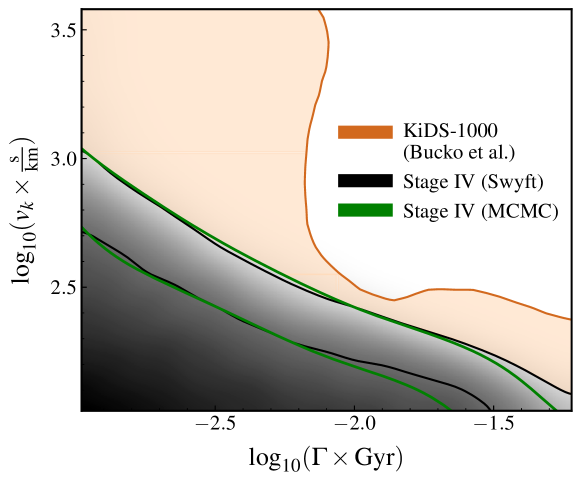
Figure 6: 95 $\%$ C.L. bounds on the $\Lambda$DDM parameters $\Gamma$ (decay rate) and $v_{k}$ (WDM velocity kick). The orange contour denotes the current strongest constraints from KiDS-1000 WL data [77], while the gray contour indicates our projected constraints from 3x2pt Stage IV photometric probes (obtained with Swyft). For comparison we also show the results obtained with MCMC (green contour). Stage IV surveys can improve the bounds on the $\Lambda$DDM model by up to one order of magnitude.

MNRE can likewise be applied to accelerate the inference of $\Lambda$CDM extensions having significantly non-Gaussian posteriors. To highlight this aspect, we analyze a model (dubbed $\Lambda$DDM) where dark matter is allowed to decay into a massless and a massive particle; the latter of these then behaves in a manner akin to warm dark matter (WDM). The phenomenology of this scenario was reviewed in detail in [78, 79], where it was shown to provide a simple way to ease the $S_{8}$ tension thanks to the time- and scale-dependent power suppression induced by the warm species. Thereafter, the $\Lambda$DDM model was tested using different LSS observables, such as the galaxy power spectrum [80], the Milky Way satellite counts [81], the Lyman-$\alpha$ forest [82] and the Sunyaev-Zel’dovich galaxy clusters [83]. Recently, the strongest bounds on this model were derived using the WL power spectra from KiDS-1000 [77].

This $\Lambda$DDM model is characterized by two extra parameters, the dark matter decay rate ($\Gamma$), and the velocity kick ($v_{k}$) received by the warm decay product, which for small velocities can be written as

$$\frac{v_{k}}{c}\simeq\frac{1}{2}\left(1-\frac{m^{2}_{\mathrm{wdm}}}{m^{2}_{\mathrm{dcdm}}}\right),$$ (4.3)

where $m_{\mathrm{dcdm}}$ and $m_{\mathrm{wdm}}$ refer to the mass of the dark matter and warm decay product, respectively. Given that $\Lambda$DDM models with large decay rates and large velocity kicks are already ruled out by observations, we focus on late-time decays ($\Gamma/H_{0}\lesssim 1$) and non-relativistic velocity kicks ($v_{k}/c\ll 1$). In this regime, the expansion history is essentially unaffected, and the main effect is a suppression in the matter power spectrum, whose cut-off scale and amplitude are controlled by $v_{k}$ and $\Gamma$, respectively [79]. In order to model the response of dark matter decays on the non-linear power spectrum, i.e. $\mathcal{S}(k,z)\equiv P^{\mathrm{nonlin}}_{\Lambda\mathrm{DDM}}(k,z)/P^{\mathrm{nonlin}}_{\Lambda\mathrm{CDM}}(k,z)$, we use the publicly available emulator DMemu that was developed in [77]. To perform the Swyft and MCMC analyses, we use almost the same setup as that described in Sec. 4.1. This time, we vary not only the $\Lambda$CDM and nuisance parameters, but also the decaying dark matter parameters, using the following priors:

$$\mathrm{log}_{10}(\Gamma\times\mathrm{Gyr}) \sim\mathcal{U}([-3.0,-1.2]),$$ (4.4)

$$\mathrm{log}_{10}(v_{k}\times\mathrm{s}/\mathrm{km}) \sim\mathcal{U}([2.0,3.6]).$$ (4.5)

The rest of parameters are varied with somewhat wider priors than in Eq. 4.2, namely $\theta_{i}\sim\mathcal{U}([\theta^{0}_{i}-6\sigma_{i}^{F},\theta^{0}_{i}+6\sigma_{i}^{F}])$, to better capture any potential new degeneracies. The mock observation is generated with the same fiducial cosmology as before, i.e. assuming no dark matter decay ($\Gamma,v_{k}\rightarrow 0$). Using the aforementioned computational resources, we generated $3\times 10^{4}$ simulations for Swyft and trained the marginal posteriors in less than $3$ hours, while the MCMC analysis took $\sim 8$ days to fully converge. The marginalized 2-dimensional posterior for $\Gamma$ and $v_{k}$ is shown in Fig. 6. We can extract two important messages. First, the Swyft and MCMC results are again in very good agreement, reinforcing the idea that Swyft can easily be applied to test alternative models exhibiting significantly non-gaussian posteriors. Secondly, the comparison with current limits shows that future Stage IV experiments can improve the bounds on the $\Lambda$DDM model by up to 1 order of magnitude. This highlights the great constraining power of surveys like Euclid on $\Lambda$CDM extensions predicting a late-time growth suppression, since these surveys will provide very precise tomographic information on the matter power spectrum.

5 Conclusions and outlook

In this work, we have shown how Marginal Neural Ratio Estimation (MNRE, as implemented in the public code Swyft) can be used to optimize cosmological parameter inference from upcoming Stage IV photometric galaxy surveys, such as Euclid or LSST. This technique offers a number of benefits compared to traditional likelihood-based methods:

1. MNRE enters in the framework of simulation-based inference (SBI) (also known as likelihood-free inference), meaning that it does not need to assume a possibly incorrect functional form for the likelihood, only to generate samples from it.

2. MNRE directly estimates the marginal posteriors of interest, so it can be much more efficient and flexible than conventional MCMC methods (as well as other SBI approaches). This is particularly advantageous when the number of nuisance parameters is very large. Moreover, the generation of simulations can be fully parallelised, and hence made extremely fast given appropriate computational resources.

3. MNRE allows to perform statistical consistency checks which are usually unfeasible for MCMC, such as coverage tests.

In order to illustrate these aspects, we have focused on the photometric 3x2pt statistics measured at 10 tomographic bins, that we have modelled with a 17-dimensional cosmological+nuisance parameter space. Our findings can be summarized as follows:

• With the training data composed of $5\times 10^{4}$ angular power spectra and the expected Stage IV experimental noise, we were able to accurately reconstruct the posterior distribution of all $\Lambda$CDM and nuisance parameters with $1-2$ orders of magnitude less computational time than MCMC. We also performed coverage tests to validate the behaviour of our estimated posteriors. Our inference pipeline is expected to yield even larger speedup factors for more refined LSS likelihoods/simulators, since an arbitrarily large number of nuisance parameters can be included without increasing the number of required simulations [35].

• In order to show that MNRE performs equally well when posteriors are highly non-Gaussian, we have investigated a non-standard model of two-body decaying dark matter that was recently proposed as a solution to the $S_{8}$ tension [78]. Using $3\times 10^{4}$ simulated power spectra as training data, we again find posteriors that are in excellent agreement with MCMC at significantly reduced computational cost. In addition, we showed that Stage IV surveys will allow to improve current limits on the two free parameters of the model by up to one order of magnitude. This illustrates that MNRE provides a powerful tool to test extended cosmologies, which is often computationally prohibitive with classical methods.

It will be interesting to extend our pipeline to include other LSS observables, such as spectroscopic galaxy clustering, and explore how constraints evolve with different combinations of probes. In fact, MNRE gives the opportunity to quickly perform massive global scans, since for a given theoretical model one can re-use simulations to perform inference for many different experimental configurations, while for MCMC one is forced to start new chains every time different observations are considered [35]. Finally, let us note that, while in this work we have focused on two-point statistics, these capture only a fraction of relevant cosmological information. In recent years, there has been a growing interest in performing inference directly with field-level LSS data, in order to extract all the information available in higher order statistics and better constrain the cosmological parameters [84, 50, 51, 56]. In future work, we plan to use MNRE to perform field-level inference of Stage IV galaxy surveys.

Appendix A Network architecture

As discussed in Sec. 4.1, we have split the network architecture for the ratio estimation into two separate components: i) a data compression network ${\bm{S}}=C_{\phi}({\bm{x}})$, which learns to compress the potentially high-dimensional data ${\bm{x}}$ into low-dimensional features ${\bm{S}}$; ii) a network to perform the actual ratio estimation, by learning to discriminate between marginally and jointly drawn model parameters ${\bm{\theta}}$ and feature vectors ${\bm{S}}$. The details of the compression network are dictated by the specific properties of the data. We recall that in our case the data can be written as a vector ${\bm{x}}=\bf{s}({\bm{\theta}})+\bf{n}$, where $\bf{s}({\bm{\theta}})$ is the concatenation of all angular spectra computed according to Eq. 3.10-Eq. 3.12, and $\bf{n}$ is a noise vector drawn from the multivariate normal distribution $\mathcal{N}(0,\mathbf{C})$, with covariance matrix $\mathbf{C}$ given by Sec. 3.2.1. We have a total of $N_{\mathrm{spectra}}=N_{\mathrm{bin},z}(2N_{\mathrm{bin},z}+1)=210$ distinct power spectra, each binned in $N_{\mathrm{bin},\ell}=29$ multipoles, so the size of the data vector ${\bm{x}}$ is $6090$. Since this vector contains a large number of correlated noisy spectra, we found beneficial to do the data compression by taking the following steps:

1. In order to decouple the different spectra, we start by performing a Cholesky decomposition of the covariance matrix, $\mathbf{C}=\mathbf{L}\mathbf{L}^{T}$ (where $\mathbf{L}$ is a lower triangular matrix), and change to the basis $\tilde{{\bm{x}}}=\mathbf{L}^{-1}{\bm{x}}$.

2. Secondly, we do a Principal Component Analysis (PCA) in order to rotate to a smaller basis capturing the largest data variations. More precisely, we construct a matrix $\mathbf{A}$ by stacking $10^{4}$ samples of the vector $\tilde{\bf{s}}=\mathbf{L}^{-1}\bf{s}$, and subsequently perform a singular value decomposition $\mathbf{A}=\mathbf{U}\mathbf{D}\mathbf{V}$, where $\mathbf{U}$ and $\mathbf{V}$ are unitary matrices and $\mathbf{D}$ is a rectangular diagonal matrix. We then project the data to the new basis $\tilde{{\bm{x}}}^{\prime}=\mathbf{V}\tilde{{\bm{x}}}$, but retaining only the first $N_{\rm PCA}$ components for which the eigenvalues contribute to more than $0.1\%$ of the total (typically $N_{\rm PCA}\sim 30-40$).

3. Thirdly, we use a linear compression network that maps the rotated data vector $\tilde{{\bm{x}}}^{\prime}$ into a feature vector ${\bm{S}}$.

Notice that the first two steps are performed only once at the beginning, while for the third step we optimize the parameters of the linear compression network during training. We assume that each parameter can be well described by 2 features, so the feature vector ${\bm{S}}$ has a size $2N_{\rm params}$, where $N_{\rm params}$ is the number of parameters of interest. We concatenate each of these parameters with the corresponding features, and fed this as input to the ratio estimators, in charge of estimating every 1- and 2-dimensional marginal posterior (see Fig. 3). Each ratio estimator is described by a multi-layer perceptron (MLP) with four layers, each containing 64 neurons.

Appendix B Coverage of the network

One of the key motivations for using MNRE is to apply it to problems in cosmology where the inference with traditional methods is extremely time-consuming, or even impossible. Hence, it is important to have additional consistency checks that do not require having a ground-truth against which to compare the results (such as the converged MCMC that we showed in Sec. 4).

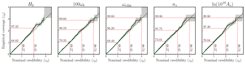
Figure 7: Coverage test for the cosmological parameters from the $\Lambda$CDM analysis of 3x2pt Stage IV photometric probes. The black solid line indicates the average coverage, while the gray contour indicates the $68\%$ uncertainty on the coverage. We see that the empirical coverage and confidence level generally match to excellent precision.

In the context of SBI, the most well established techniques are known as coverage tests. This sort of methods exploits the fact that, once the inference networks are trained, they can effortlessly generate the posteriors for any mock observation simulated from the prior (as opposed to MCMC, where one gets the posterior for a single observation). Hence, the idea is to perform inference on many different mock data simulations to get the empirical coverage, which gives the proportion of time that a certain interval contains the true parameter value. For a well-calibrated posterior, the $p\%$ credible interval should contain the simulation-truth value $p\%$ of the time, so one should get a totally diagonal line when plotting the empirical coverage against the expected credible intervals. These tests are generally unfeasible for sequential sampling methods such as MCMC, where one needs to rely on convergence criteria like the Gelman-Rubin statistic [75]. However, it should be noted that coverage tests provide a necessary but not sufficient condition for the calibration of the posteriors. Developing new tests in order to trust results from SBI is an active area of ongoing research [91, 92].

Using a batch of 500 simulations, we perform the coverage test for the marginal posteriors of the five $\Lambda$CDM parameters trained in Sec. 4.2. Instead of showing the highest posterior density region $p$, we choose to work with a new variable $z_{p}$ defined by $p/100=\frac{1}{\sqrt{2\pi}}\int_{-z_{p}}^{z_{p}}dz\exp{(-z^{2}/2)}$, to place more emphasis in the tail of the posteriors. This means that the $(1,2,3)\sigma$ regions correspond to $z_{p}=(1,2,3)$ with $p=(68.27,95.45,99.97)$. We also compute the uncertainty on the empirical coverage arising from the finite sample size, using the Jeffreys interval (see [35] for details). The results of the test are shown in Fig. 7. We find that for every parameter, we achieve excellent posterior coverage, which adds additional validation to our agreement with MCMC.

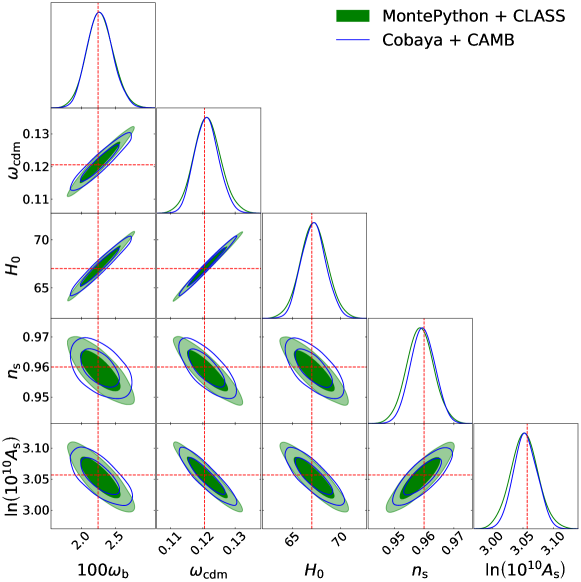
Figure 8: Constraints on the cosmological parameters from 3x2pt Stage IV photometric probes. We show the difference between two codes using a similar implementation of the Metropolis-Hastings algorithm: Cobaya (blue, with CAMB as the Boltzmann solver) and MontePython (green, with CLASS as the Boltzmann solver). The red dashed lines indicate the injected values.

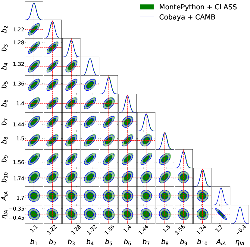
Figure 9: Constraints on the nuisance parameters from 3x2pt Stage IV photometric probes. We show the difference between two codes using a similar implementation of the Metropolis-Hastings algorithm: Cobaya (blue, with CAMB as the Boltzmann solver) and MontePython (green, with CLASS as the Boltzmann solver). The red dashed lines indicate the injected values.

Appendix C Comparison between MontePython+CLASS and Cobaya+CAMB

In order to double-check our methodology, we have conducted the MCMC analyses using two distinct combinations of software tools: MontePython with CLASS and Cobaya with CAMB. As shown in Fig. 8 and 9, we find excellent agreement between these different codes. This underscores the reliability and robustness of both MCMC pipelines, and reinforces the idea that the main advantages found with Swyft still hold regardless of which MCMC pipeline is used. It also suggests that either combination can be safely utilized for further comparisons with Swyft (i.e. Swyft can be trained using simulations from CLASS or CAMB).

References

- [1] Planck collaboration, Planck 2018 results. VI. Cosmological parameters, Astron. Astrophys. 641 (2020) A6 [1807.06209].
- [2] E. Abdalla et al., Cosmology intertwined: A review of the particle physics, astrophysics, and cosmology associated with the cosmological tensions and anomalies, JHEAp 34 (2022) 49 [2203.06142].
- [3] R. Laureijs, J. Amiaux, S. Arduini, J.L. Auguères, J. Brinchmann, R. Cole et al., Euclid Definition Study Report, arXiv e-prints (2011) arXiv:1110.3193 [1110.3193].
- [4] Euclid collaboration, Euclid preparation: VII. Forecast validation for Euclid cosmological probes, Astron. Astrophys. 642 (2020) A191 [1910.09273].
- [5] LSST Science Collaboration, P.A. Abell, J. Allison, S.F. Anderson, J.R. Andrew, J.R.P. Angel et al., LSST Science Book, Version 2.0, arXiv e-prints (2009) arXiv:0912.0201 [0912.0201].
- [6] LSST Dark Energy Science collaboration, The LSST Dark Energy Science Collaboration (DESC) Science Requirements Document, 1809.01669.
- [7] J. Lesgourgues, The Cosmic Linear Anisotropy Solving System (CLASS) I: Overview, 1104.2932.
- [8] D. Blas, J. Lesgourgues and T. Tram, The Cosmic Linear Anisotropy Solving System (CLASS) II: Approximation schemes, JCAP 07 (2011) 034 [1104.2933].
- [9] A. Lewis, A. Challinor and A. Lasenby, Efficient computation of CMB anisotropies in closed FRW models, Astrophys. J. 538 (2000) 473 [astro-ph/9911177].
- [10] C. Howlett, A. Lewis, A. Hall and A. Challinor, CMB power spectrum parameter degeneracies in the era of precision cosmology, JCAP 04 (2012) 027 [1201.3654].
- [11] DES collaboration, Dark Energy Survey Year 3 Results: Photometric Data Set for Cosmology, Astrophys. J. Suppl. 254 (2021) 24 [2011.03407].
- [12] DES collaboration, Dark Energy Survey Year 3 results: Cosmological constraints from galaxy clustering and weak lensing, Phys. Rev. D 105 (2022) 023520 [2105.13549].
- [13] K.K. Rogers, H.V. Peiris, A. Pontzen, S. Bird, L. Verde and A. Font-Ribera, Bayesian emulator optimisation for cosmology: application to the Lyman-alpha forest, JCAP 02 (2019) 031 [1812.04631].
- [14] Euclid collaboration, Euclid preparation: IX. EuclidEmulator2 – power spectrum emulation with massive neutrinos and self-consistent dark energy perturbations, Mon. Not. Roy. Astron. Soc. 505 (2021) 2840 [2010.11288].
- [15] A. Spurio Mancini, D. Piras, J. Alsing, B. Joachimi and M.P. Hobson, CosmoPower: emulating cosmological power spectra for accelerated Bayesian inference from next-generation surveys, Mon. Not. Roy. Astron. Soc. 511 (2022) 1771 [2106.03846].
- [16] S. Günther, J. Lesgourgues, G. Samaras, N. Schöneberg, F. Stadtmann, C. Fidler et al., CosmicNet II: emulating extended cosmologies with efficient and accurate neural networks, JCAP 11 (2022) 035 [2207.05707].
- [17] M. Bonici, L. Biggio, C. Carbone and L. Guzzo, Fast emulation of two-point angular statistics for photometric galaxy surveys, 2206.14208.
- [18] A. Nygaard, E.B. Holm, S. Hannestad and T. Tram, CONNECT: a neural network based framework for emulating cosmological observables and cosmological parameter inference, JCAP 05 (2023) 025 [2205.15726].
- [19] K. Cranmer, J. Brehmer and G. Louppe, The frontier of simulation-based inference, Proc. Nat. Acad. Sci. 117 (2020) 30055 [1911.01429].
- [20] F. Villaescusa-Navarro et al., Multifield Cosmology with Artificial Intelligence, 2109.09747.
- [21] F. Villaescusa-Navarro et al., Robust marginalization of baryonic effects for cosmological inference at the field level, 2109.10360.
- [22] X. Zhao, Y. Mao, C. Cheng and B.D. Wandelt, Simulation-based Inference of Reionization Parameters from 3D Tomographic 21 cm Light-cone Images, Astrophys. J. 926 (2022) 151 [2105.03344].
- [23] M. Dax, S.R. Green, J. Gair, J.H. Macke, A. Buonanno and B. Schölkopf, Real-Time Gravitational Wave Science with Neural Posterior Estimation, Phys. Rev. Lett. 127 (2021) 241103 [2106.12594].
- [24] M. Crisostomi, K. Dey, E. Barausse and R. Trotta, Neural posterior estimation with guaranteed exact coverage: The ringdown of GW150914, Phys. Rev. D 108 (2023) 044029 [2305.18528].
- [25] D.B. Rubin, Bayesianly Justifiable and Relevant Frequency Calculations for the Applied Statistician, The Annals of Statistics 12 (1984) 1151 .
- [26] T. Toni, D. Welch, N. Strelkowa, A. Ipsen and M.P.H. Stumpf, Approximate bayesian computation scheme for parameter inference and model selection in dynamical systems, Journal of The Royal Society Interface 6 (2009) 187 .
- [27] G. Papamakarios, D. Sterratt and I. Murray, Sequential neural likelihood: Fast likelihood-free inference with autoregressive flows, in Proceedings of he 22nd International Conference on Artificial Intelligence and Statistics, pp. 837–848, PMLR, Apr., 2019.
- [28] G. Papamakarios and I. Murray, Fast -free inference of simulation models with bayesian conditional density estimation, in Advances in Neural Information Processing Systems, pp. 1028–1036, Dec., 2016.
- [29] N. Jeffrey and B.D. Wandelt, Solving high-dimensional parameter inference: marginal posterior densities & Moment Networks, in 34th Conference on Neural Information Processing Systems, 11, 2020 [2011.05991].
- [30] K. Cranmer, J. Pavez and G. Louppe, Approximating Likelihood Ratios with Calibrated Discriminative Classifiers, 1506.02169.
- [31] J. Hermans, V. Begy and G. Louppe, Likelihood-free MCMC with amortized approximate ratio estimators, in Proceedings of the 37th International Conference on Machine Learning, vol. 119, pp. 4239–4248, PMLR, Jul, 2020.
- [32] J. Alsing, B. Wandelt and S. Feeney, Massive optimal data compression and density estimation for scalable, likelihood-free inference in cosmology, Mon. Not. Roy. Astron. Soc. 477 (2018) 2874 [1801.01497].
- [33] J. Alsing, T. Charnock, S. Feeney and B. Wandelt, Fast likelihood-free cosmology with neural density estimators and active learning, Mon. Not. Roy. Astron. Soc. 488 (2019) 4440 [1903.00007].
- [34] B.K. Miller, A. Cole, P. Forré, G. Louppe and C. Weniger, Truncated Marginal Neural Ratio Estimation, in 35th Conference on Neural Information Processing Systems, 7, 2021, DOI [2107.01214].
- [35] A. Cole, B.K. Miller, S.J. Witte, M.X. Cai, M.W. Grootes, F. Nattino et al., Fast and credible likelihood-free cosmology with truncated marginal neural ratio estimation, JCAP 09 (2022) 004 [2111.08030].
- [36] A. Saxena, A. Cole, S. Gazagnes, P.D. Meerburg, C. Weniger and S.J. Witte, Constraining the X-ray heating and reionization using 21-cm power spectra with Marginal Neural Ratio Estimation, Mon. Not. Roy. Astron. Soc. 525 (2023) 6097 [2303.07339].
- [37] K. Karchev, R. Trotta and C. Weniger, SICRET: Supernova Ia Cosmology with truncated marginal neural Ratio EsTimation, 2209.06733.
- [38] K. Karchev, M. Grayling, B.M. Boyd, R. Trotta, K.S. Mandel and C. Weniger, SIDE-real: Truncated marginal neural ratio estimation for Supernova Ia Dust Extinction with real data, 2403.07871.
- [39] N.A. Montel, A. Coogan, C. Correa, K. Karchev and C. Weniger, Estimating the warm dark matter mass from strong lensing images with truncated marginal neural ratio estimation, Mon. Not. Roy. Astron. Soc. 518 (2022) 2746 [2205.09126].
- [40] A. Coogan, N. Anau Montel, K. Karchev, M.W. Grootes, F. Nattino and C. Weniger, The effect of the perturber population on subhalo measurements in strong gravitational lenses, Mon. Not. Roy. Astron. Soc. 527 (2024) 66 [2209.09918].
- [41] N. Anau Montel and C. Weniger, Detection is truncation: studying source populations with truncated marginal neural ratio estimation, in 36th Conference on Neural Information Processing Systems: Workshop on Machine Learning and the Physical Sciences, 11, 2022 [2211.04291].
- [42] J. Alvey, M. Gerdes and C. Weniger, Albatross: a scalable simulation-based inference pipeline for analysing stellar streams in the Milky Way, Mon. Not. Roy. Astron. Soc. 525 (2023) 3662 [2304.02032].
- [43] U. Bhardwaj, J. Alvey, B.K. Miller, S. Nissanke and C. Weniger, Sequential simulation-based inference for gravitational wave signals, Phys. Rev. D 108 (2023) 042004 [2304.02035].
- [44] J. Alvey, U. Bhardwaj, S. Nissanke and C. Weniger, What to do when things get crowded? Scalable joint analysis of overlapping gravitational wave signals, 2308.06318.
- [45] J. Alvey, U. Bhardwaj, V. Domcke, M. Pieroni and C. Weniger, Simulation-based inference for stochastic gravitational wave background data analysis, 2309.07954.
- [46] P.L. Taylor, T.D. Kitching, J. Alsing, B.D. Wandelt, S.M. Feeney and J.D. McEwen, Cosmic Shear: Inference from Forward Models, Phys. Rev. D 100 (2019) 023519 [1904.05364].
- [47] N. Jeffrey, J. Alsing and F. Lanusse, Likelihood-free inference with neural compression of DES SV weak lensing map statistics, Mon. Not. Roy. Astron. Soc. 501 (2021) 954 [2009.08459].
- [48] J. Fluri, T. Kacprzak, A. Lucchi, A. Schneider, A. Refregier and T. Hofmann, Full wCDM analysis of KiDS-1000 weak lensing maps using deep learning, Phys. Rev. D 105 (2022) 083518 [2201.07771].
- [49] K. Lin, M. von Wietersheim-Kramsta, B. Joachimi and S. Feeney, A simulation-based inference pipeline for cosmic shear with the Kilo-Degree Survey, Mon. Not. Roy. Astron. Soc. 524 (2023) 6167 [2212.04521].
- [50] DES collaboration, Dark Energy Survey Year 3 results: likelihood-free, simulation-based CDM inference with neural compression of weak-lensing map statistics, 2403.02314.
- [51] P. Lemos et al., SimBIG: Field-level Simulation-Based Inference of Galaxy Clustering, in 40th International Conference on Machine Learning, 10, 2023 [2310.15256].
- [52] C. Hahn, M. Eickenberg, S. Ho, J. Hou, P. Lemos, E. Massara et al., : The First Cosmological Constraints from the Non-Linear Galaxy Bispectrum, 2310.15243.
- [53] J. Hou, A. Moradinezhad Dizgah, C. Hahn, M. Eickenberg, S. Ho, P. Lemos et al., : Cosmological Constraints from the Redshift-Space Galaxy Skew Spectra, 2401.15074.
- [54] C. Modi and O.H.E. Philcox, Hybrid SBI or How I Learned to Stop Worrying and Learn the Likelihood, 2309.10270.
- [55] B. Tucci and F. Schmidt, EFTofLSS meets simulation-based inference: from biased tracers, 2310.03741.
- [56] N.-M. Nguyen, F. Schmidt, B. Tucci, M. Reinecke and A. Kostić, How much information can be extracted from galaxy clustering at the field level?, 2403.03220.
- [57] N. Metropolis, A.W. Rosenbluth, M.N. Rosenbluth, A.H. Teller and E. Teller, Equation of state calculations by fast computing machines, J. Chem. Phys. 21 (1953) 1087.
- [58] J. Skilling, Nested Sampling, AIP Conf. Proc. 735 (2004) 395.
- [59] D. Foreman-Mackey, D.W. Hogg, D. Lang and J. Goodman, emcee: The MCMC Hammer, Publ. Astron. Soc. Pac. 125 (2013) 306 [1202.3665].
- [60] M.S. Vogeley and A.S. Szalay, Eigenmode analysis of galaxy redshift surveys I. theory and methods, Astrophys. J. 465 (1996) 34 [astro-ph/9601185].
- [61] D. Coe, Fisher Matrices and Confidence Ellipses: A Quick-Start Guide and Software, 0906.4123.
- [62] R. Trotta, Bayes in the sky: Bayesian inference and model selection in cosmology, Contemporary Physics 49 (2008) 71 [0803.4089].
- [63] B. Audren, J. Lesgourgues, K. Benabed and S. Prunet, Conservative Constraints on Early Cosmology: an illustration of the Monte Python cosmological parameter inference code, JCAP 1302 (2013) 001 [1210.7183].
- [64] J. Torrado and A. Lewis, Cobaya: Code for Bayesian Analysis of hierarchical physical models, JCAP 05 (2021) 057 [2005.05290].
- [65] D.N. Limber, The Analysis of Counts of the Extragalactic Nebulae in Terms of a Fluctuating Density Field. II, Astrophys. J. 119 (1954) 655.
- [66] B. Joachimi et al., Galaxy alignments: An overview, Space Sci. Rev. 193 (2015) 1 [1504.05456].
- [67] A. Kiessling et al., Galaxy Alignments: Theory, Modelling \& Simulations, Space Sci. Rev. 193 (2015) 67 [1504.05546].
- [68] D. Kirk et al., Galaxy alignments: Observations and impact on cosmology, Space Sci. Rev. 193 (2015) 139 [1504.05465].
- [69] Euclid Collaboration, D. Sciotti, S. Gouyou Beauchamps, V.F. Cardone, S. Camera, I. Tutusaus et al., Euclid preparation. TBD. Forecast impact of super-sample covariance on 3x2pt analysis with Euclid, arXiv e-prints (2023) arXiv:2310.15731 [2310.15731].
- [70] A. Mead, C. Heymans, L. Lombriser, J. Peacock, O. Steele and H. Winther, Accurate halo-model matter power spectra with dark energy, massive neutrinos and modified gravitational forces, Mon. Not. Roy. Astron. Soc. 459 (2016) 1468 [1602.02154].
- [71] A. Mead, S. Brieden, T. Tröster and C. Heymans, HMcode-2020: Improved modelling of non-linear cosmological power spectra with baryonic feedback, 2009.01858.
- [72] VIRGO Consortium collaboration, Stable clustering, the halo model and nonlinear cosmological power spectra, Mon. Not. Roy. Astron. Soc. 341 (2003) 1311 [astro-ph/0207664].
- [73] T. Simon, P. Zhang, V. Poulin and T.L. Smith, Consistency of effective field theory analyses of the BOSS power spectrum, Phys. Rev. D 107 (2023) 123530 [2208.05929].
- [74] E.B. Holm, L. Herold, T. Simon, E.G.M. Ferreira, S. Hannestad, V. Poulin et al., Bayesian and frequentist investigation of prior effects in EFT of LSS analyses of full-shape BOSS and eBOSS data, Phys. Rev. D 108 (2023) 123514 [2309.04468].
- [75] A. Gelman and D.B. Rubin, Inference from Iterative Simulation Using Multiple Sequences, Statist. Sci. 7 (1992) 457.
- [76] A. Lewis, GetDist: a Python package for analysing Monte Carlo samples, 1910.13970.
- [77] J. Bucko, S.K. Giri, F.H. Peters and A. Schneider, Probing the two-body decaying dark matter scenario with weak lensing and the cosmic microwave background, 2307.03222.
- [78] G. Franco Abellán, R. Murgia, V. Poulin and J. Lavalle, Implications of the tension for decaying dark matter with warm decay products, Phys. Rev. D 105 (2022) 063525 [2008.09615].
- [79] G. Franco Abellán, R. Murgia and V. Poulin, Linear cosmological constraints on two-body decaying dark matter scenarios and the S8 tension, Phys. Rev. D 104 (2021) 123533 [2102.12498].
- [80] T. Simon, G. Franco Abellán, P. Du, V. Poulin and Y. Tsai, Constraining decaying dark matter with BOSS data and the effective field theory of large-scale structures, Phys. Rev. D 106 (2022) 023516 [2203.07440].
- [81] DES collaboration, Milky Way Satellite Census. IV. Constraints on Decaying Dark Matter from Observations of Milky Way Satellite Galaxies, Astrophys. J. 932 (2022) 128 [2201.11740].
- [82] L. Fuß and M. Garny, Decaying Dark Matter and Lyman- forest constraints, JCAP 10 (2023) 020 [2210.06117].
- [83] H. Tanimura, M. Douspis, N. Aghanim and J. Kuruvilla, Testing decaying dark matter models as a solution to the S8 tension with the thermal Sunyaev-Zel’dovich effect, Astron. Astrophys. 674 (2023) A222 [2301.03939].
- [84] A. Andrews, J. Jasche, G. Lavaux and F. Schmidt, Bayesian field-level inference of primordial non-Gaussianity using next-generation galaxy surveys, Mon. Not. Roy. Astron. Soc. 520 (2023) 5746 [2203.08838].
- [85] C.R. Harris et al., Array programming with NumPy, Nature 585 (2020) 357 [2006.10256].
- [86] J.D. Hunter, Matplotlib: A 2D Graphics Environment, Comput. Sci. Eng. 9 (2007) 90.
- [87] A. Paszke et al., PyTorch: An Imperative Style, High-Performance Deep Learning Library, 1912.01703.
- [88] W. Falcon and T.P.L. team, Pytorch lightning, Zenodo (2024), DOI.
- [89] Joblib Development Team, Joblib: running python functions as pipeline jobs, (2020), https://joblib.readthedocs.io/.
- [90] T. Kluyver, B. Ragan-Kelley, F. Pérez, B. Granger, M. Bussonnier, J. Frederic et al., Jupyter Notebooks—a publishing format for reproducible computational workflows, in IOS Press, pp. 87–90 (2016), DOI.
- [91] J. Hermans, A. Delaunoy, F. Rozet, A. Wehenkel, V. Begy and G. Louppe, A Trust Crisis In Simulation-Based Inference? Your Posterior Approximations Can Be Unfaithful, 2110.06581.
- [92] P. Lemos, A. Coogan, Y. Hezaveh and L. Perreault-Levasseur, Sampling-based accuracy testing of posterior estimators for general inference, 40th International Conference on Machine Learning 202 (2023) 19256 [2302.03026].