Connection between galaxy morphology and dark-matter halo structure I: a running threshold for thin discs and size predictors from the dark sector

Abstract

We present a series of studies on the connection between galaxy morphology and the structure of host dark-matter (DM) haloes using cosmological simulations. In this work, we introduce a new kinematic decomposition scheme that features physical identification of morphological components, enabling robust separation of thin and thick discs; and measure a wide range of halo properties, including their locations in the cosmic web, internal structures, and assembly histories. Our analysis of the TNG50 simulation reveals that the orbital-circularity threshold for disc differentiation varies across galaxies, with systematic trends in mass and redshift, so the widely used decomposition method with constant circularity cuts is oversimplified and underestimates thin disc at JWST redshifts. The energy threshold between the stellar halo and the inner galaxy is also a function of mass and redshift, minimizing at the sub-Galactic halo mass, where the circularity threshold peaks. Revisiting the issue of galaxy size predictor, we show that disc sizes in TNG50 exhibit correlations with three structural parameters besides virial mass and redshift: 1) a positive correlation with halo spin $\lambda$ across redshifts – stronger than previously reported for zoom-in simulations but still weaker than the simple $r_{1/2}/R_{\rm vir}\propto\lambda$ scaling; 2) an anti-correlation with DM concentration $c$ that is well described by $r_{1/2}/R_{\rm vir}\propto c^{-0.7}$ even when $c$ is measured in the DM only run; 3) more actively accreting haloes having slightly larger discs, as well as more significant stellar haloes and lower thin-to-thick ratio. Disc mass fraction is higher in rounder haloes and in cosmic knots and filaments, implying that disc development needs both stable halo conditions and continuous material supply. Our methodology is public and adaptable to other simulations.

1 Introduction

In the standard paradigm of cosmic structure formation, dark-matter (DM) haloes provide the sites for galaxy formation. Galaxies show dramatic structural diversity across redshifts, and the diversity intensifies at the mass regime of bright dwarf galaxies. It is natural to speculate that the morphologies of galaxies contain information of host DM haloes, and that the structural diversity of the haloes is correlated with that of the inhabitant galaxies. The halo virial mass determine many galactic properties statistically, not only the stellar mass (e.g., Yang et al., 2003, 2008, 2012; Behroozi et al., 2013; Moster et al., 2013), but also various aspects of galaxy morphology. Notably, the size of a galaxy is approximately $\sim 2\%$ of the virial radius (e.g., Kravtsov, 2013; Somerville et al., 2018) (which is equivalent to halo mass at a given epoch); and galactic angular momentum (AM) has also been shown in cosmological hydro simulations to stabilize after the halo reaches a characteristic mass scale, above which both stellar feedback and disc instability weaken (Dekel et al., 2020a; Hopkins et al., 2023). Besides halo mass, which secondary properties of the DM halo are most relevant in regulating galactic morphology has become a pivotal question in understaning galaxy-halo connection and galaxy evolution (e.g., Hearin et al., 2013; Behroozi et al., 2019; Chen et al., 2021) that all semi-analytical and semi-empirical frameworks of galaxy evolution need to address.

For example, semi-analytical models (SAMs) assign disc sizes to star-forming galaxies according to certain dark-matter halo properties. The classical prescription based on AM conservation is that disc size relative to halo size is proportional to the spin parameter $\lambda$ of the host halo (Fall & Efstathiou, 1980; Mo et al., 1998), which, in turn, can be predicted by the tidal torque theory (White, 1984) or obtained from cosmological $N$-body simualtions. This motivates some SAMs to predict the sizes of star-forming discs as $r_{\rm 1/2}\sim\lambda R_{\rm vir}$, where $R_{\rm vir}$ is the virial size of the host halo and $\lambda$ the instantaneous halo spin (e.g., Somerville et al., 2008). Other SAMs compute disc size using the disc AM accumulated over time from that of the circum-galactic medium, which in turn depends on some time average of the halo spin (e.g., Benson, 2012). Such recipes, with the cosmological average spin of DM haloes being $\sim 0.03$, agrees with the observed proportionality between galaxy sizes and halo sizes as inferred from abundance matching (Kravtsov, 2013). Galactic bulges form as major mergers of disc galaxies occur and bulge sizes reflect energy conservation during the mergers. Thus in almost all SAMs, disc galaxies are prevalent before bulges emerge. As such, the explanation of the morphological diversity of star-forming (dwarf) galaxies with SAMs is basically that, the most compact galaxies and the most diffuse galaxies populate DM haloes of the lowest and highest spin, respectively, by construction. However, some cosmological hydro simulations reveal a largely orthogonal story compared to the standard SAM view, in the sense that, in simulations, disc morphology is rare and unstable at high redshifts when cosmic accretion is intense, and when star formation and stellar feedback is bursty. It is after the formation of a central compact stellar bulge (or other forms of compact mass distribution) that long-lived, extended discs start to develop (Dekel et al., 2020a; Hafen et al., 2022; Yu et al., 2023; Hopkins et al., 2023). Accordingly, the morphological diversity of galaxies in these simulations are not tied to the AM content of the haloes, but may be related to other structural parameters (e.g., Jiang et al., 2019).

Galactic morphological diversity is not merely in terms of disc size, but also in terms of the mass ratios and detailed properties of different morphological components, including thin disc, thick disc, bulge, and stellar halo. Investigations of galaxy morphology is hindered by the difficulty in cleanly separating different morphological components. Even with cosmological simulations, where straightforward morphological decomposition based on the kinematics of stars is feasible, it is still not clear how to define the aforementioned components using self-consistent physical criteria. For example, the most widely used kinematic decomposition method would designate the stars with an orbital circularity above a fixed arbitrary threshold value as thin-disc stars (e.g., Yu et al., 2021, 2023; Genel et al., 2015; Tacchella et al., 2019; Sotillo-Ramos et al., 2023). Similar arbitrary thresholds exist for thick discs and spheroidal components. Different studies use different threshold values, and have different rules for assigning stars to different components, hindering efficient comparisons and reproducibility. Hence, to investigate the connections between galaxy morphology and DM halo structures, and to facilitate meaningful comparisons amongst different simulations, we first need to clarify morphological definitions and minimize arbitrariness in them.

The structural parameters of DM haloes include not merely the AM structure and the density-profile shape. They at least also include the 3D triaxial shape (Jing & Suto, 2002), and broadly speaking, the mass assembly histories as well as the cosmological large-scale environments (e.g., Wang et al., 2007; Wang et al., 2011; Wang et al., 2018; Shi et al., 2015). Haloes acquire their AM from large-scale tidal torques (White, 1984), and gain broken power-law density profiles from fast accretion in the early Universe followed by slow build-up of the outskirt at later times (e.g., Zhao et al., 2003, 2009; Ludlow et al., 2013). The 3D shapes also contain information of the cosmic web at large (Forero-Romero et al., 2014; Ganeshaiah Veena et al., 2018). Hence, the instantaneous structure of a DM halo are correlated with both its assembly history and the cosmic environment. It is natural to expect that galaxy morphology also contains information of these spatial and temporal factors (see e.g., Mo et al., 2023).

In this series of studies, we work towards a comprehensive exploration of the relationship between galactic morphology and the broadly-defined DM-halo structural properties. In particular, we aim at sorting out the answers to the following questions:

• Can we simplify kinematic morphological decomposition of simulated galaxies into a robust and non-arbitrary workflow?

• Which DM-halo parameters are most tightly correlated with a chosen galaxy morphological parameter? For example, what halo properties constitute the best predictor for disc size?

• To what extent can we use DM halo properties alone to predict the morphological properties of the inhabitant galaxies? For example, from the point of view of semi-analytical or semi-empirical modeling, is it feasible at all to paint galaxies to haloes using a collection of secondary halo parameters, especially given that galaxies are shaped also by their own internal baryonic processes and that the DM may be redistributed by these processses (e.g., Blumenthal et al., 1986; Gnedin et al., 2004; Pontzen & Governato, 2013)?

This work (Paper I) addresses the first question and also touches base on the second question. In paper II, we address morphology-halo relations in more detail, with the help of machine-learning algorithms.

Paper I is organized as follows. In Section 2, we describe the morphological and structural quantities that we measure for the simulated galaxies. In Section 3, we introduce our new kinematic decomposition scheme and comment on some insights that are immediately clear with this method. We present a few correlations between galaxy morphological parameters and halo structural parameters in Section 4, with an emphasis on which halo properties affect disc size. Different decomposition methods are compared in Section 5, and we summarize this study in Section 6. Throughout this study, we focus on central galaxies unless otherwise stated, and define haloes as spherical overdensities that are 200 times the critical density of the Universe, and assume cosmological parameters adopted in the simulations analyzed.

2 Simulation Catalog and Measurements

To extract statistical galaxy-halo connections that involve detailed morphological information from cosmological hydro-simulations, we need a simulation sample with both cosmologically meaningful box size and adequate numerical resolution. In this work, we use the highest resolution run of the Illustris-TNG suite, TNG50 (Pillepich et al., 2019; Nelson et al., 2019), which has a gas particle mass of $10^{4.93}M_{\odot}$, a DM particle mass of $10^{5.65}M_{\odot}$, and a gravitational softening length for collisionless (gas) particles of 0.288 (0.074) comoving kpc. We limit our analysis to the galaxies with a half-stellar-mass radius at least two times the collisionless softening length, and those with more than 1000 stellar particles as well as 1000 DM particles within virial radius. We use the galaxies and haloes in the public catalogs, for which haloes are identified with the Friends-of-Friends (FoF, Davis et al., 1985) and SUBFIND (Springel et al., 2001) algorithms, and are linked accross snapshots with the SUBLINK merger tree algorithm (Rodriguez-Gomez et al., 2015). For certain analysis, we use DM haloes in the DM-only simulation of the same initial conditions and focus on the haloes that have a matched counterpart in the hydro-simulation according to the public Subhalo Matching To Dark catalog . To reveal potential redshift trends, we analyze the simulations at $z=0$, 1, 2, and 4. We use the halo catalogs mostly only for obtaining the global properties such as halo mass and galaxy mass. For the structural parameters, we perform measurements using the particle data and our in-house developed programs that are highly modular, so that such measurements can be easily extended to other simulations in the future for comparisons. We make our measurements as well as our particle-data reduction pipeline publicly available at https://github.com/JinningLianggithub/MorphDecom. Below, we list all the structural parameters considered in this study and describe their operational definitions, summarized in Table 1.

Halo quantities	Description	Reference
Halo concentration $c$	$c=R_{\rm vir}/r_{-2}$ based on fitting Einasto profile	Einasto (1965)
Halo spin $\lambda$	$j_{\rm vir}/(\sqrt{2}R_{\rm vir}V_{\rm vir})$	Bullock et al. (2001)
Late-time accretion parameter $\beta$	as in $M_{\rm vir}(z)\propto(1+z)^{\beta}e^{-\gamma z}$, MAH slope at late times	McBride et al. (2009)
Early-time accretion parameter $\gamma$	as in $M_{\rm vir}(z)\propto(1+z)^{\beta}e^{-\gamma z}$, MAH slope at early times	McBride et al. (2009)
Halo axis ratio $q$	ratio between intermediate axis and major axis $b/a$ calculated from eigenvalues of shape tensors	Allgood et al. (2006)
Environment	location in cosmic web as knot, filament, sheet or void, based on local eigenvalues of tidal shear tensor	Hahn et al. (2007)
Galaxy (stellar-particle) quantities	Description	Reference
Size $r_{\rm 1/2}$	3D radius within which the enclosed stellar mass is equal to half of total stellar mass within the halo	public TNG50 catalog
Normalized specific binding energy $e_{\rm b}$	Specific binding energy, $E$, scaled by the absolute value of $E$ of the most bound particle, $|E|_{\rm max}$	Doménech-Moral et al. (2012)
Circularity $\eta$	Azimuth specific AM $j_{z}$ scaled by the maximal AM with the same binding energy $j_{\rm circ}(E)$	Abadi et al. (2003)
Polarity $\epsilon$	Non-azimuth specific AM $j_{\rm p}$ scaled by the maximal AM with the same binding energy $j_{\rm circ}(E)$	Doménech-Moral et al. (2012)
Circularity threshold $\eta_{\rm cut}$	Intersection of the $\eta$ distributions of the two discy components found by the Gaussian Mixture Models algorithm – for separating thin and thick discs	This work
Energy threshold $e_{\rm cut}$	Local minimum in the $e_{\rm b}$ distribution – for separating high-energy and low-energy stellar components	Zana et al. (2022)
Mass fraction $f_{X}$	$f_{\rm X}=M_{\star,X}/M_{\star}$, where $M_{\star,X}$ is the mass of morphological component $X$

Table 1: Structural parameters of DM haloes and morphological quantities of galaxies (as well as kinematics quantities of stellar particles) used in this study.

2.1 Dark-Matter Halo Quantities

• Halo mass and virial radius $M_{\rm vir}$ is defined as the enclosed total mass within the sphere of radius $R_{\rm vir}$, the radius within which the average total density is $\Delta$ times the critical density of the Universe, with $\Delta=200$, consistent with the definition used for the SUBFIND catalog.

• The circular velocity is defined as $V_{\rm circ}=\sqrt{GM_{\rm dm}(<r)/r}$, where $M_{\rm dm}(<r)$ is the enclosed DM mass within radius $r$. The maximum circular velocity, $V_{\rm max}$, is the maximum value of the $V_{\rm circ}(r)$, and $r_{\rm max}$ is the radius at which $V_{\rm circ}(r)=V_{\rm max}$. Note that the definitions for $V_{\rm max}$ and $r_{\rm max}$ are different from those in the public SUBFIND catalog, the latter of which are based on the total mass profiles.

• Halo concentration describes the compactness of the DM halo and reflects the depth of the gravitational potential well at fixed halo mass, defined as $c=R_{\rm vir}/r_{-2}$, where $r_{-2}$ is scale radius at which the logarithmic densty slope is $-2$. To measure concentration, the most commonly used approach is to perform parametric fits to the density profile, assuming, e.g., the Navarro et al. (1997, hereafter NFW) functional form. Haloes are more accurately described by the Einasto (1965) profile,

  $$\rho_{\rm Einasto}=\rho_{-2}\exp\left\{-2n\left[\left(\frac{r}{r_{-2}}\right)^{1/n}-1\right]\right\},$$ (1)

  at the expense of just one additional parameter compared to NFW. This additional degree of freedom is important for capturing baryonic and environmental impacts on halo structure. Here, $\rho_{-2}$ is the density at $r_{-2}$, linked to the virial mass via $\rho_{-2}=M_{\rm vir}/(4\pi h^{3}n\gamma(3n,x(R_{\rm vir}))$, with $h\equiv r_{-2}/(2n)^{n}$, $\gamma(a,x)$ the non-normalized incomplete gamma function, and $x\equiv 2n(r/r_{-2})^{1/n}$. We have experimented with different measurements of halo concentration, including parametric fits of NFW and Einasto functional forms, and non-parametric proxies constructed using $V_{\rm max}$ and $r_{\rm max}$, $\tilde{V}_{\rm max}$, as proposed by Bose et al. (2019), as well as a straightforward $c=R_{\rm vir}/r_{-2}$, with the scale radius $r_{-2}$ measured from the density profile. We find that the concentration based on fitting the Einasto circular velocity profile carries the least fitting error and yields the strongest correlations with galaxy morphologies, and thus use it as the default definition for concentration. We note that the Dekel-Zhao profile (Freundlich et al., 2020) is better suited for describing halo response, and has the same degree of freedom as Einasto. However, here for concentration measurement, we stick to Einasto as it is the more common choice in this context.

• The halo spin parameter is defined as $\lambda=j_{\rm vir}/(\sqrt{2}R_{\rm vir}V_{\rm vir})$, following Bullock et al. (2001), where $j_{\rm vir}$ is the specific AM within the virial radius, and $V_{\rm vir}$ is the circular velocity at virial radius.

• The mass assembly history (MAH) of a DM halo is defined as the mass of the main branch progenitor as a function of redshift, $M_{\rm vir}(z)$. The MAHs from the simulations are arrays of length up to the total number of snapshots, and are thus not straightforward to use in the search for correlations between galaxy morphology and halo MAH. To reduce the dimension of MAHs, we fit the MAHs using the functional form introduced by McBride et al. (2009),

  $$M_{\rm vir}(z)=M_{\rm vir}(1+z)^{\beta}e^{-\gamma z},$$ (2)

  where $\beta$ and $\gamma$ are the two free parameters describing the speed of halo growth at late and early times, respectively. Here the exponential growth is an analytic prediction in the EdS regime (Dekel et al., 2013), and the later power-law redshift dependence is an empirical results based on simulations. We use $\beta-\gamma$ as a proxy for the recent accretion rate, because the accretion rate

  $$\frac{\text{d}\ln{M_{\rm vir}(z)}}{\text{d}z}=\frac{\beta}{1+z}-\gamma$$ (3)

  is approximately $\beta-\gamma$ at $z\sim 0$. At higher redshift, it can be also shown that the average accretion rate within a dynamical time is strongly correlated with $\beta-\gamma$. As already discussed in McBride et al. (2009), MAHs can be classified according to the value of $\beta-\gamma$. The more actively accreting a halo is, the more negative $\beta-\gamma$ is. For haloes that are halted in mass growth or have started losing mass, $\beta-\gamma\ga 0$. Hence, while we focus on central haloes, we regard $\beta-\gamma>0$ as an implication of backsplash or at least an indicator of environmental influence.

  

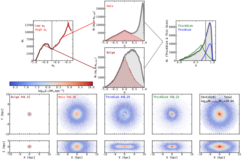
  Figure 1: Illustration of our new decomposition method, with a Milky-Way-mass galaxy at $z$=0. Upper panels: the distributions of specific binding energy $e_{\rm b}$ and circularity $\eta$. In the left panel, the thick gray curve stands for the $e_{\rm b}$ distribution of the whole galaxy, with the brighter red curve marking the high-energy component and darker red curve standing for the low-energy component, separated by the vertical gray line indicating the threshold $e_{\rm cut}$. In the upper middle column, we show the circularity distributions of the low-energy and high-energy components, respectively – the bulge and stellar halo correspond to the symmetric distributions highlighted in red, where the positive $\eta$ parts are obtained from Monte Carlo sampling. For the remaining stellar particles, as indicated by the gray shaded $\eta>0$ areas in the middle columns and combined in the right panel, they are first classified into two subgroups with the GMM algorithm, and are further split into thin and thick discs according to the threshold $\eta_{\rm cut}$. The green and blue lines are the smoothed Gaussian components provided by GMM, whose intersection is used as the threshold $\eta_{\rm cut}$. Lower panels: face-on and edge-on views of the resulting bulge, halo, thin disc, and thick disc components, coloured by surface density, with the galaxy ID and its stellar mass within 5 half-stellar-mass radius quoted.

• The 3D shape of DM haloes can be characterized by the eigen-values of the inertia tensor (Allgood et al., 2006),

  $$\mathcal{S}=\frac{1}{M}\sum_{k}m_{k}\bm{r}_{k,i}\bm{r}_{k,j},$$ (4)

  where the summation is over all the DM particles within the ellipsoid of interest, $\bm{r}_{k,i}$ is the component of the position vector of the $k$th particle along axis $i$, and $M=\Sigma_{k}m_{k}$ is the total mass within the ellipsoid. The eigenvalues of $\mathcal{S}$ are proportional to the squares of the semi-axes ($a\geq b\geq c$) of the ellipsoid that describes the spatial distribution of the particles. We measure the eigenvalues iteratively, starting from the virial sphere until convergence, following the algorithm of Tomassetti et al. (2016). The shapes are expressed in terms of the 3D axis ratios, e.g., $q=b/a$ and $p=c/b$.

  	$F_{V}$				$F_{M}$				$N_{\rm cen}$
  Redshift	Knot	Filament	Sheet	Void	Knot	Filament	Sheet	Void	Knot	Filament	Sheet	Void
  0	0.005	0.137	0.367	0.491	0.350	0.374	0.191	0.085	150	1297	3136	506
  1	0.006	0.116	0.342	0.536	0.223	0.353	0.268	0.156	160	1603	3620	596
  2	0.006	0.094	0.311	0.588	0.128	0.304	0.322	0.246	166	1646	3464	650
  4	0.004	0.056	0.237	0.703	0.041	0.180	0.332	0.447	76	758	1768	427

  Table 2: Volume fraction, mass fraction and number of TNG50 central galaxies residing in knots, filaments, sheets, and voids at different redshifts.

• The large-scale environment of a DM halo can be characterized as the position within the cosmic web. We classify cosmic web using the eigenvalues of the deformation tensor (e.g., Hahn et al., 2007; Forero-Romero et al., 2009), $T_{i,j}$. Based on the analysis of large-scale structures using the Zel’dolvich approximation, cosmic web can be classified by counting the number of eigenvalues of the deformation tensor exceeding a threshold $\lambda_{\rm th}$ (chosen to be 0.4 in this work, see below), such that 0, 1, 2, or 3 eigenvalues exceeding $\lambda_{\rm th}$ corresponds to void, sheet, filament, or knot, respectively. To determine the tidal tensor $T_{i,j}$ and the eigenvalues at each coordinate, we follow the steps laid out in Martizzi et al. (2019), adapting the public code complementary to the work of Yang et al. (2022). In particualr, first, starting from the Poisson equation:

  $$\nabla^{2}\phi(\bm{x})=4\pi G\bar{\rho}\delta(\bm{x}),$$ (5)

  where $G$ is the gravitational constant, $\bar{\rho}(z)$ is the mean matter density of the Universe, and $\delta(\bm{x})\equiv\rho(\bm{x})/\bar{\rho}-1$ is the overdesnity, we compute the overdensity field by interpolating the mass of each particle to a $512^{3}$ Cartesian grid using a cloud-in-cell method smoothed by a Gaussian filter of scale $R_{\rm G}=0.5$ckpc$h^{-1}$. Second, to facilitate the computation of the tidal tensor, we express the gravitational potential in units of $4\pi G\bar{\rho}$ such that eq. (5) becomes simply $\nabla^{2}\phi(\bm{x})=\delta(\bm{x})$. With the Fourier transform of the overdensity field, $\delta_{\bm{k}}$, we can compute the Fourier transform of the tidal tensor as

  $$\Psi_{i,j,\bm{k}}=k_{i}k_{j}\phi_{\bm{k}},\ \ i,j=1,2,3,$$ (6)

  where $k_{i}$ is wave number in Fourier space. By performing the inverse FFT of $\Psi_{i,j,\bm{k}}$ for each $(i,j)$, one can obtain the deformation tensor element $T_{i,j}(\bm{x})$ at each point in the original space. Finally, we solve

  $$\text{det}\left(\bm{T}(\bm{x})-\lambda(\bm{x})\bm{I}\right)=0$$ (7)

  for the eigenvalues $\lambda_{1}(\bm{x})>\lambda_{2}(\bm{x})>\lambda_{3}(\bm{x})$. The parameter values of $\lambda_{\rm th}=0.4$ and $R_{G}=0.5$ cMpc$h^{-1}$ are chosen based on our visual comparison of the resulting cosmic-web classification and the density map of the simulation, and are in the same ballpark as the values reported in the literature (e.g., Martizzi et al., 2019).

2.2 Galaxy Quantities

• Half-stellar-mass radius $r_{\rm 1/2}$ is the 3D radius within which the enclosed stellar mass is equal to half of total stellar mass within the halo, provided by the public TNG50 catalog.

• Stellar mass $M_{\star}$ – instead of considering all the stellar particles within the virial radius, we define stellar mass as the stellar mass within 5$r_{\rm 1/2}$. We have verified that this can exclude most of the merger relics of satellite galaxies but at the same time retaining most of the smooth stellar halo of the central galaxies. We exclude the wind particles in TNG50 from the stellar mass.

• Parameters for kinematic morphological decomposition – circularity $\eta$, polartiy $\epsilon$, and normalized binding energy $e_{\rm b}$

  We base our morphological decomposition on the energy structure and AM structure of the stellar particles within 5$r_{\rm 1/2}$. We present the workflow of our method in Section 3, but define the relevant quantities here. For each stellar particle, we consider two AM related parameters, the circularity $\eta$ and the polarity $\epsilon$, as well as one energy parameter, $e_{\rm b}$, defined as follows. Circularity is the ratio of the azimuthal AM $j_{z}$ to the maximum AM $j_{\rm circ}(E)$, where $j_{z}=\bm{j}\cdot\hat{\bm{z}}$, with $\hat{\bm{z}}$ the unit vector of the total AM of the galaxy (calculated with all the stellar particles within 5$r_{\rm 1/2}$), and $j_{\rm circ}(E)$ is the AM of a circular orbit of the same specific orbital energy $E$ as the particle of interest has. $j_{\rm circ}(E)$ is obtained by following its definition, $j_{\rm circ}(E)=r_{\rm c}(E)V_{\rm circ}(E)$, where $V_{\rm circ}(E)$ is the circular velocity at given specific orbital energy $E$, and $r_{\rm c}(E)$ is the radius of this circular orbit. The details of $j_{\rm circ}(E)$ evaluation are given in Section 3. The counterpart of circularity for the polar component of the AM, $\bm{j_{\rm p}}=\bm{j}-\bm{j_{\rm z}}$, is denoted by $\epsilon\equiv j_{\rm p}/j_{\rm circ}(E)$, which we dub the polarity parameter (e.g., Doménech-Moral et al., 2012). The normalized specific binding energy $e_{\rm b}$ measures how bound a stellar particle is, and is defined as $e_{\rm b}=E/|E|_{\rm max}$, where $|E|_{\rm max}$ is the absolute value of the specific energy of the most bound particle.

• The mass fraction of a morphological component is given by $f_{\rm X}=M_{\star,X}/M_{\star}$ where $M_{\star,X}$ is the mass of morphogical component $X$ (bulge, stellar halo, thin disc, or thick disc), the identification of which is detailed in Section 3.

3 A New Morphological Decomposition Procedure

Most previous studies on kinematic morphological decomposition adopt constant thresholds in circularity (e.g., Yu et al., 2021, 2023; Genel et al., 2015; Tacchella et al., 2019; Sotillo-Ramos et al., 2023), and many just simply assign the star particles below certain circularity to bulge, and those with $\eta\ga 0.7$ to disc, without considering the energy structure of stellar mass. Zana et al. (2022) improves this simple scheme by first considering a local minimum in the energy distribution to split star particles into a high-energy population and a dynamically colder population, which contain the stellar halo and bulge, respectively, and then uses a constant circularity threshold to further identify the discs. That is, a physically clear criterion is used in the energy space, but the circularity criteria is still arbitrarily constant. The difficulty for a self-consistent criteria in the AM space is simply that there is usually no clear local minimum in the circularity distribution. However, in the 3D parameter space spanned by $\eta$, $\epsilon$, and $e_{\rm b}$, star particles can be more clearly separated into different groups. Du et al. (2019) has demonstrated this using a unsupervised machine-learning approach: they first split stars into several groups in the 3D space, before assigning them into different morphological components according to whether the median circularities and median energies of the groups fall into the $\eta$ and $e_{\rm b}$ regimes that define the morphological components. But again, constant and arbitrary circularity thresholds (as well as energy thresholds) are used.

Incorporating the wisdom in Zana et al. (2022) and Du et al. (2019), here we introduce a new decomposition scheme, minimizing the arbitrariness in these methods. Basically, we use the Gaussian-Mixture-Models algorithm (GMM, as implemented in the Python package scikit-learn) to separate thin and thick discs, after applying a Zana et al. style energy cut and identifying the bulge and stellar halo. We enforce GMM to search for two groups in the $\eta$-$\epsilon$-$e_{\rm b}$ space after removing the random-motion supported bulge and halo, and find that GMM can robustly return us a higher-$\eta$ group, which corresponds to the thin disc, and a lower-circularity (and usually also higher-energy) subsystem, which corresponds to the thick disc. The detailed procedure is as follows.

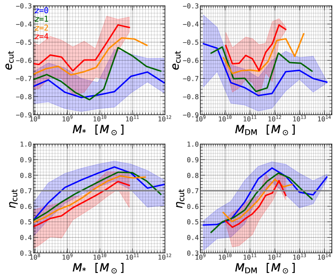
Figure 2: The energy threshold $e_{\rm cut}$ (upper) and orbital-circularity threshold $\eta_{\rm cut}$ (lower) for morphological decomposition, as a function of galaxy stellar mass (left) or DM halo mass (right), at different redshifts, as indicated. The blue and red bands indicate the 16th and 84th percentiles for redshift 0 and 4, respectively. The variances at given mass are similar for other two redshifts and are thus not shown to avoid crowdedness. The horizontal gray lines in the lower panels represent the widely-used constant circularity threshold for separating thin and thick disc, $\eta_{\rm cut}=0.7$. Both thresholds vary systematically with mass and redshift, with peak $\eta_{\rm cut}$ and minimal $e_{\rm cut}$ occuring at the characteristic halo mass scale of $M_{\rm vir}\sim 10^{11.5-12}M_{\odot}$, insensitive to redshift.

• Use the subhalo position from the TNG50 subhalo catalog, which is the location of the particle of the minimum gravitational potential, as galaxy centre.

• In order to compute energy and AM for kinematic decomposition, one needs to know the specific potential energy of each particle. This information is not readily available in the TNG particle data, so we re-evaluate the potential of a galaxy using all its particles using the KDTree algorithm pytreegrav. We normalize the potential by setting that of the farthest particle to zero. This is effectively equivalent to setting the potential to zero at the virial radius.

• Compute the AM of the galaxy from the stellar particles within 5$r_{\rm 1/2}$, and rotate the galaxy such that the $z$ axis is aligned with the AM vector.

• Set 100 logarithmically spaced bins of the cylindrical radius $R=\sqrt{x^{2}+y^{2}}$, between the galaxy centre and the farthest particle. For each bin, we compute the gravitational potential $\Phi_{\rm circ}$ and the gravitational acceleration $\bm{a}_{\rm circ}$ using KDTree at four positions, $(x,y,z)=$ $(R,0,0)$, $(0,R,0)$, $(-R,0,0)$, $(0,-R,0)$ and take the average values of the four measurements as the values for $\Phi_{\rm circ}$ and $\bm{a}_{\rm circ}$. With the gravitational acceleration in the galactic plane, we calculate the circular velocity, $V_{\rm circ}=\sqrt{|\bm{a}_{\rm circ}\times\bm{r}_{\rm circ}|}$, the specific circular AM, $j_{\rm circ}=RV_{\rm circ}$, and the specific binding energy in the galactic plane, $E_{\rm circ}=V_{\rm circ}^{2}/2+\Phi_{\rm circ}$. Thus we obtain a profile of $j_{\rm circ}(E_{\rm circ})$, which we turn into an interpolation function and use it to get the $j_{\rm circ}$ of individual particles given their $E_{\rm circ}$, as measured in Step 2.

• For each stellar particle, we calculate the normalized specific binding energy $e_{\rm b}$, circularity $\eta$, and polarity $\epsilon$, per their definitions (Section 2.2).

• Remove unbound ($e_{\rm b}\geq 0$) particles and rare particles of extreme values of circularity and polarity of $|\eta|\geq 1.5$ and $|\epsilon|\geq 1.5$.

• Look for a local minimum in the $e_{\rm b}$ distribution, register the corresponding $e_{\rm b}$ value as $e_{\rm cut}$, the energy threshold for separating stellar halo from the bulge. Here, we mostly follow the method of Zana et al., but revise it to better accommodate dwarf galaxies with small numbers of stellar particles. In Appendix B, we recap their method and detail our improvements.

• Split stellar particles into a more bound component, $e_{\rm b}\leq e_{\rm cut}$, and a less bound component, $e_{\rm b}>e_{\rm cut}$. The stellar halo and bulge are identified as the random-motion supported subsets of the less bound and the more bound components, respectively. Since these spheroidal components are expected to have zero net rotation, we identify them as the particle distributions symmetric about $\eta=0$. In particular, we identify the negative-circularity part and its mirrored distribution about $\eta=0$, and draw the $\eta>0$ particles to be assigned to the spheroidal components from the mirrored distributions via Monte Carlo sampling.

• With the spheroids determined, we collect the remaining stellar particles altogether regardless of their binding energy – these particles all have positive circularity and thus belong to discs. We identify a circularity threshold, $\eta_{\rm cut}$, to split them into thick and thin discs (if they both exist). Naturally, similar to the search for a energy threshold, $e_{\rm cut}$, the idea is to obtain a threshold in the circularity distribution. As stated, quite often there is no local minimum in the one-point function of circularity. Hence, we split the stars into two groups in the 3D phase space spanned by $\eta$, $\epsilon$, and $e_{\rm b}$ using GMM, by enforcing two Gaussian components. Appendix C provides further details on how the GMM algorithm operates and Appendix D shows an example of gaussian components in $\eta$-$\epsilon$-$e_{\rm b}$ space. The GMM fit is performed 10 times with different initialization for robust classification (Du et al., 2019). Next, we identify the intersection of the circularity distribution of the two Gaussian components as the threshold $\eta_{\rm cut}$. The stellar particles with $\eta\geq\eta_{\rm cut}$ are then assigned to the thin disc and the rest are thick-disc particles. If no intersection point is detected, which can happen when one of the two Gaussian components is significantly subdominant, then all the positive-circularity particles are assigned to the thin disc.

• Finally, we measure the density profiles and calculate the shape parameters of different morphological components for future work. The details will be presented in Paper II. To ensure accurate measurements, we impose that each spheroidal (disky) component should have at least 30 (100) star particles. We redistribute particles between bulge and halo or between thin disc and thick disc if the particle of a certain component is below the minimum value, e.g., if a bulge has fewer than 30 particles, the bulge is absorbed into the stellar halo. If the numbers of star particles of the thin disc and the thick disc are both below 30, they will be re-assigned to bulge or halo based on whether their $e_{\rm b}$ is below or above $e_{\rm cut}$.

Fig. 1 illustrates our morphological decomposition method with an example of a Milky-Way-mass disc galaxy ($M_{\star}=10^{10.64}M_{\odot}$). As one can see in the upper left panel, our procedure successfully identifies the most pronounced local minimum in the energy distribution at $e_{\rm cut}\simeq-0.68$, and ignores smaller local minima. The middle column in the upper panel shows the stellar halo and the stellar bulge, as the two components with symmetric circularity distributions centred around $\eta\sim 0$. The remaining stars that have positive circularity are combined, as shown in the upper right panel. In this representative case, there is no local minimum in the circularity distribution, while the GMM algorithm successfully identifies two distinct groups in the 3D $\eta$-$\epsilon$-$e_{\rm b}$ space. The two groups have circularity distributions intersecting at $\eta\simeq 0.8$, which we adopt as the circularity threshold, $\eta_{\rm cut}$. In the lower panels of Fig. 1, we show the stellar surface density maps of the four components and the whole galaxy. The mass fractions of the bulge, the stellar halo, the thin disc, and the thick disc are 0.15, 0.38, 0.25, 0.22, respectively. In Appendix A we show more examples for different kinds of systems, including rare extreme cases such as bulgeless discs and pure spheroids. We have manually inspected many representative cases of the decomposition results based on the aforementioned procedure and find it to be quite robust.

Using our methods, the kinematic-decomposition thresholds are no longer arbitrary constants, but are values that vary from one galaxy to another, reflecting the dynamical status of the system as well as various other factors. Interestingly, both $\eta_{\rm cut}$ and $e_{\rm b}$ systematically vary with galaxy mass, DM-halo mass, and redshift, as shown in Fig. 2. For example, the energy threshold $e_{\rm cut}$ decreases from the dwarf mass range ($M_{\star}\la 10^{9}M_{\odot}$ and $M_{\rm vir}\la 10^{10.5}M_{\odot}$) to sub-Galactic scale ($M_{\star}\sim 10^{9.5}M_{\odot}$ and $M_{\rm vir}\sim 10^{11.5}M_{\odot}$), and increases sharply at $M_{\rm vir}\ga 10^{12}M_{\odot}$. The physical meaning of $e_{\rm cut}$ is straightforward: it is a measurement of how bound is the dynamically cold part of the galaxy. The lower $e_{\rm cut}$ is, the more settled the galaxy is, and the more extended the outskirt stellar halo is. This V-shaped $e_{\rm cut}$-mass relation at $M_{\rm vir}<10^{12.5}M_{\odot}$ can be interpreted as follows. At the massive end ($M_{\rm vir}\ga 10^{12}M_{\odot}$), many haloes are still actively accreting and are not completely virialized, this makes $e_{\rm cut}$ high. At the low-mass end, although only central galaxies are included in this analysis, dwarf galaxies are generally more affected by environmental processes and are more contaminated by backsplash satellites. Environmental processes also drive $e_{\rm cut}$ high, with tidal processes reshaping and truncating the energy distribution so that the zero-potential surface shrinks. The redshift trend of $e_{\rm cut}$ also lends support to these interpretations – $e_{\rm cut}$ is higher at higher $z$ when both effects are more intense. At the most massive end though ($M_{\rm vir}\ga 10^{12.5}M_{\odot}$), $e_{\rm cut}$ seems to decrease with mass again, but we caution against overinterpreting this trend, as the massive end suffers from small-number statistics with the TNG50 sample.

More interesting is the relation of the circularity threshold $\eta_{\rm cut}$ with mass, as shown in the lower panels of Fig. 2. Note that $\eta_{\rm cut}$ is a gauge of how coherent is the AM of the thin disc, or simply put, how thin is the thin disc. This should be distinguished from $f_{\rm thin}$, the thin-disc mass fraction, because it can happen that a disc is thin but not significant in mass. We can see that $\eta_{\rm cut}$ increases with mass from $\sim 0.5$ at the dwarf scale to $\sim 0.8$ at roughly the Milky-Way mass, $M_{\star}\sim 10^{10.5}M_{\odot}$ or $M_{\rm vir}\sim 10^{12}M_{\odot}$, and decreases towards higher masses. That is, the Milky-Way mass coincides with the mass scale at which coherent thin discs settle.

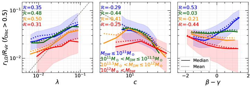
Figure 3: Galaxy compactness (galaxy half-stellar mass radius in units of host-halo virial radius) as a function of halo spin $\lambda$ (left), halo concentration $c$ (middle), and halo mass-assembly-history parameter $\beta-\gamma$ (right) for disc-dominated ($f_{\rm disc}>0.5$) central galaxies in different halo mass bins in the TNG50 simulations. The lines stand for the median or the average relations, as indicated, and the coloured bands indicate the 16th to 84th percentiles of the galaxy-compactness distribution at given fixed halo parameter (shown only for the lowest and highest mass bins to avoid making the plots too crowded). The results for redshifts 0, 1, 2, and 4 are combined to enhance statistics. Pearson correlation coefficients $\mathcal{R}$ are quoted. Gray dashed lines provide references of $r_{\rm 1/2}/R_{\rm vir}\propto\lambda$ and slope $r_{\rm 1/2}/R_{\rm vir}\propto c^{-0.7}$ in left and middle panels, respectively.

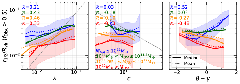
Figure 4: The same as Fig. 3 but with halo properties ($R_{\rm vir}$, $\lambda$, $c$, and $\beta-\gamma$) measured in the DM-only simulations, TNG50-dark. Results are shown for the galaxies with matched DM-only counterparts.

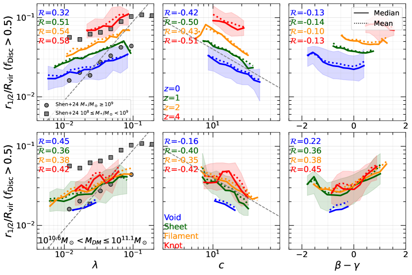
Figure 5: Similar to Fig. 3 but binning galaxies with given halo mass of $M_{\rm vir}=10^{10.6-11.1}M_{\odot}$ by redshifts (upper) and environments (lower panels). With both halo mass and redshift fixed, the concentration dependence of the form of $r_{\rm 1/2}/R_{\rm vir}\propto c^{-0.7}$ is clearer, and the correlation with halo accretion rate parameter ($\beta-\gamma$) is better revealed. Overplotted for comparison in gray squares and circles are the high-redshift ($z\ga 5.5$) results of the THESAN-HR simulation, digitized and adapted from Shen et al. (2024, see text) – the spin dependence is similar.

This characteristic scale of thin disc formation is more clear in terms of halo mass. Dekel et al. (2020a) discovered with zoom-in hydro-cosmological simulations that galactic discs become stable only when the host galaxies reach $M_{\rm vir}\ga 10^{11.5}M_{\odot}$, and that this characteristic mass is nearly redshift-independent. Our findings here with a much larger statistical sample support this picture, in the sense that the halo mass at which the thin-disc threshold peaks is basically the same as that reported by Dekel et al. for disc settlement, and is similarly almost insensitive to redshift. The peak value $\eta_{\rm cut}$ is redshift dependent though, but this simply reflects the fact that discs are generally less settled at higher $z$ when accretion is more intense and that the AM directions are constantly affected by the AM supply in the cosmic web. Dekel et al. attribute disc stabilization at $M_{\rm vir}\ga 10^{11.5}M_{\odot}$ to a process they dub gas-rich compaction. This process gives rise to a compact star-forming bulge that stabilizes the disc (see Dekel et al., 2020b; Lapiner et al., 2023, for a thorough discussion). While the TNG50 simulation lacks the resolution to fully resolve the compaction process, what we find here implies that the same behavior holds qualitatively. The decrease of $\eta_{\rm cut}$ at the galaxy-group scale likely reflects disc-thickening due to frequent heating by mergers and secular evolution. To consolidate these speculations is beyond the scope of current work. Here, we conclude that simplistic decomposition with constant $\eta_{\rm cut}$ of $\sim 0.7$ would overestimate thin discs for Milky-Way-mass galaxies, and underestimate thin discs for dwarfs.

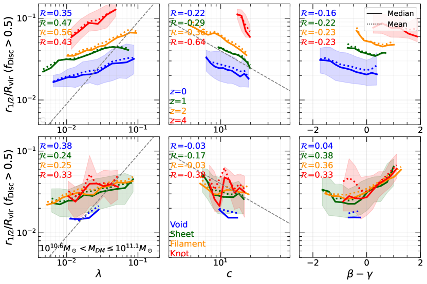
Figure 6: The same as Fig. 5 but with halo properties measured in the DM-only simulations, TNG50-dark. Results are shown for the galaxies with matched DM-only counterparts.

4 Galaxy morphology and halo structure

With different morphological components identified, we study how galaxy morphology is related to the structures of their hosting DM haloes. First, we identify the leading factors affecting the sizes of disc-dominated galaxies (Section 4.1). Second, we explore the dependence of the mass ratios of different morphological components on halo properties (Section 4.2).

4.1 Disc-size predictor revisited

The sizes of disc galaxies have been a pivotal topic in galaxy formation theory and simulations. However, there is no consensus yet on, first, which properties of the DM halo besides the virial mass (or virial radius) is most tightly correlated with the size of the inhabitant disc; second, whether it is plausible at all to accurately predict disc size using DM properties alone – a question taking centre stage in semi-analytical models of galaxy evolution. With the assumption of AM conservation during galaxy formation, Mo et al. (1998) shows that thin exponential discs populating NFW haloes have a size of

$$r_{\rm 1/2}\simeq f_{j}\lambda R_{\rm vir}$$ (8)

where $f_{j}=j_{\mathrm{gal}}/j_{\mathrm{halo}}$ is the AM retention factor, i.e., how much of the specific AM of the cold baryonic component is inherited from the DM halo, usually assumed to be a constant of order unity. As such, the galactic disc size is explicitly linked to the spin of the host halo, serving as a convenient prescription of galaxy size in galaxy-formation models. However, an investigation of zoom-in cosmological hydro simulations (Jiang et al., 2019) reveals that the halo spin parameter has marginal correlation with the AM content of the inhabitant galaxies and therefore exhibits negligible predicting power for galaxy size, at least at high redshifts ($z\ga 1$). Instead, an empirical relation of galaxy size with the halo concentration parameter was shown to agree with the simulation results,

$$r_{\rm 1/2}\simeq 0.02(1+z)^{-0.2}c_{10}^{-0.7}R_{\rm vir},$$ (9)

where $c_{10}$ is concentration in multiples of the typical value of 10 for Milky-Way mass haloes at $z\sim 0$. This empirical relation captures the redshift dependence of galaxy sizes partially via the cosmological concentration-mass-redshift relation. The physical prediction of Mo et al. has no explicit redshift dependence, but an implicit one may arise via the AM retention factor. Both models contain a leading-order dependence of disc size on the virial radius, $r_{\rm 1/2}\sim 0.02R_{\rm vir}$, as found by abundance-matching results at low $z$ (Kravtsov, 2013; Somerville et al., 2018). Since the halo radius (mass) is undoubtedly the dominant factor for galaxy size and is shared by these models, below, we focus on the ratio $r_{\rm 1/2}/R_{\rm vir}$ and explore which secondary halo parameters are correlated with this ratio. We call this ratio the galaxy compactness with respect to the host halo.

As shown in Fig. 3, the spin parameter $\lambda$ is indeed positively correlated with $r_{\rm 1/2}/R_{\rm vir}$, almost insensitive to the mass range of interest. However, the average relation is shallower than $r_{\rm 1/2}/R_{\rm vir}\propto\lambda$. The correlation of galaxy size with spin is notably stronger than that found in Jiang et al. (2019), which is based on zoom-in simulations of higher resolution than TNG50. We note that even in the two zoom-in suites that Jiang et al. analyzed, the lower-resolution NIHAO sample exhibits somewhat stronger correlation with halo spin than that in the higher-resolution VELA sample, especially at low $z$ (see Fig.A1 therein). These imply that numerical resolution might play a role in connecting the AM of the galaxy and that of the host halo. Different stellar feedback prescriptions amongst these simulations could also impact the AM connection, as well as other aspects of galaxy-halo structural connections. The results shown here only reflect the TNG50 simulation and are not necessarily generic. For example, depending on the detailed implementation of feedback in a simulation, the fraction of gas turned into stars may sample the total halo gas very differently, and the correlation between galaxy size with halo spin may be different in simulations where the coupling of the gas and the feedback energy is modeled differently.

There is almost no redshift dependence on the correlation strength with halo spin, as can be seen from the upper left panel of Fig. 5. Shen et al. (2024) studied galaxy size in the THESAN-HR simulations in the reionization epoch, and actually found a very similar level of correlation strength with halo spin, as overlayed in Fig. 5 for comparison. The THESAN-HR simulation features on-the-fly radiative transfer (RT), and adopts otherwise similar subgrid prescriptions to TNG50. Hence, we infer that real-time RT does not play a crucial role in establishing or eliminating the spin dependence, but other aspects of feedback might, given that both TNG50 and THESAN-HR exhibit similarly strong $\lambda$ dependence, stronger than that in the NIHAO and VELA suites.

With the larger sample of TNG50, we verify the anti-correlation between disc compactness and halo concentration first revealed with zoom-in simulations. This trend is actually quite close to the $c^{-0.7}$ scaling as previously found if imposing a simple power law dependence, at least for lower-mass haloes of $M_{\rm vir}\la 10^{12}M_{\odot}$, and seems to be weaker for the more massive ones. There is a noticeable flattening of this trend at the low-concentration end, which we refrain from over-interpreting because of the limited statistics and the unrelaxed nature of haloes with very low concentration.

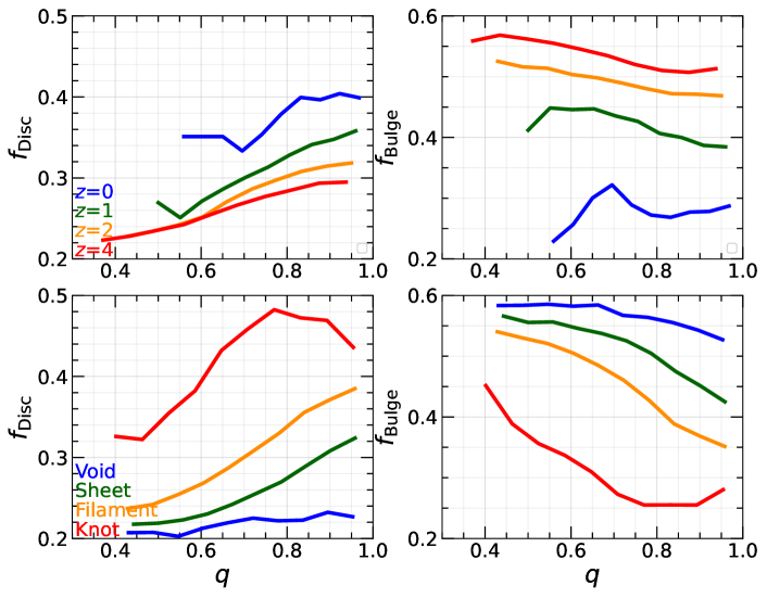
Figure 7: The median mass fraction of discs (left) and bulges (right) as a function of halo shape $q$ for central galaxies at different redshifts (upper) or in different environments (lower). Here we focus on the median trend, but note that the scatter in $f_{X}$ at fixed halo axis ratio $q$ is actually large, comparable to the vertical plotting range.

A negative $c$ dependence may arise from adiabatic contraction of DM haloes in response to the inhabitant disc potentials. To test this scenario, we use the DM-only (DMO) run and focus on haloes with matched counterparts between the DMO run and the full-physics run. We measure their stellar properties in the hydro run, and the DM properties including $R_{\rm vir}$, $\lambda$, and $c$ are from the matched haloes in the DMO run. The results are shown in Fig. 4, where we can see that the $c$ dependence is indeed somewhat weakened, implying that it arises partially from halo response. However, there is still a residual negative correlation between $r_{\rm 1/2}/R_{\rm vir}$ and the DMO concentration. We try to further clarify the trend with $c$ by keeping both the halo mass and redshift fixed, as shown in Fig. 6. We choose the mass bin of $M_{\rm vir}=10^{10.6-11.1}M_{\odot}$ in order to have both decent statistics and a mass range that is sufficiently narrow to rule out contamination from mass dependence. Clearly, the same concentration scaling basically holds for haloes of the narrow mass bin and at fixed redshift. We conclude that, while the concentration dependence is weaker than the spin dependence, it is not purely a consequence of halo response so that $c$ from DMO simulations still have predicting power on galaxy size.

Besides halo spin and concentration, the MAH of the halo also affects disc size, as shown in the last column of Figs. 3-6. Here, we have parameterized the MAH by the parameter combination $\beta-\gamma$, which, as introduced in Section 2.1, reflects the overall shape of the MAH, and approximates the accretion rate at redshift zero. From Figs. 3 and 4, the relations between galaxy compactness $r_{\rm 1/2}/R_{\rm vir}$ and $\beta-\gamma$ seems to be complicated: at face value, the correlation is positive for the lowest mass bin of $M_{\rm vir}\leq 10^{11}M_{\odot}$, and flips sign for more massive haloes. This positive correlation for low-mass haloes is however a trivial manifestation of the following factors. First, higher-$z$ galaxies are generally more extended with respect to their host haloes. Second, the possible range of $\beta-\gamma$ is a function of redshift such that for higher $z$, $\beta-\gamma$ is generally larger. These are illustrated in the upper right panels of Fig. 5 and Fig. 6. These panels also confirm that there is still an intrinsic MAH dependence of disc compactness at fixed halo mass and redshift, in the sense that in the more actively accreting haloes (which have more negative $\beta-\gamma$), galaxies are more extended. This correlation is rather weak, with a Pearson coefficient of $\cal{R}\simeq$ -0.13 and $\simeq-0.23$ in the hydro run and DMO run respectively, but holds robustly throughout redshifts.

Finally, we explore the impact of environment on these correlations by dividing the galaxies according to their cosmic-web identities, as shown in the lower panels of Fig. 5-6. There is no clear-cut trends with cosmic-web environments. Galaxies in denser environments seem to be slightly more extended than those in voids, but we caution against interpreting this due to the low statistics in voids.

4.2 Mass fractions of morphological components

The mass ratios of different morphological components also correlate with host-halo properties. Notably, the disc fraction $f_{\rm disc}$ correlates positively with the 3D axis ratio $q$ of DM haloes, as shown in the left column of Fig. 7. The axis ratio $q$ is an indicator of how relaxed a system is (Schneider et al., 2012; Bonamigo et al., 2015; Menker & Benson, 2022), and we have verified that other traxiality indicators (i.e., shape parameters involving combinations of $q$ and $p$) or relaxedness indicators (e.g., $T/|U|$, the ratio between kinetic and potential energy) yields qualitatively similar trends. Hence, relaxed and rounder systems ($q\sim 1$) tend to host more significant discs. The bulge fraction $f_{\rm bulge}$, on the other hand, correlates negatively with halo shape $q$, in the sense that the bulge fraction is higher in more elongated systems. Both trends are weak and of large scatter, but are robust against binning the samples by redshift or cosmic-web environment. The redshift and environmental trends are both straightforward to understand, that lower-redshift and knot galaxies are more disc dominated, coherent with the picture that disc formation needs more settled environments.

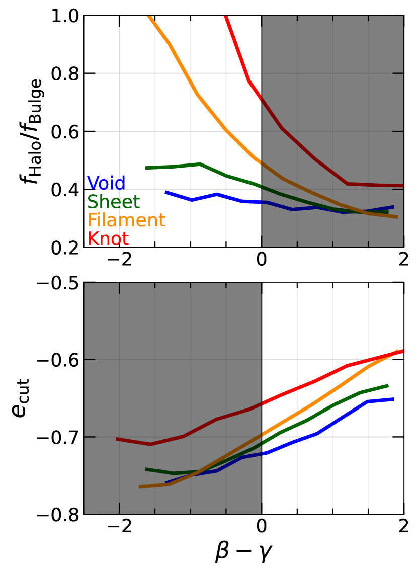
Figure 8: The median mass ratio between stellar halo and bulge (upper), and the median energy threshold $e_{\rm cut}$ (lower), as a function of accretion-rate proxy $\beta$-$\gamma$ at different cosmic-web locations. For $f_{\rm halo}/f_{\rm bulge}$ and $e_{\rm cut}$, we focus on the growing regime ($\beta-\gamma<0$) and environmentally-limited regime ($\beta-\gamma>0$), respectively, where clearer trends can be identified.

The mass ratio between the stellar halo and the stellar bulge, $f_{\rm halo}/f_{\rm bulge}$, measures how significant is the dynamically hotter component relative to the colder stellar component, and also depends on DM halo properties, as shown in Fig. 8. Here we focus on the regime of $\beta-\gamma<0$, i.e., focus on the systems that still grow. The more actively accreting the DM halo (i.e., the smaller $\beta-\gamma$ is), the more significant the hotter stellar component. This manifests that active accretion brings in more satellite galaxies which contributes their stripped stars to the stellar halo of the host system. This correlation shows a clear environmental dependence, such that it is strongest in cosmic knots and that the halo-to-bulge ratio is generally higher in knots.

Closely related to the mass ratio, $f_{\rm halo}/f_{\rm bulge}$, is the energy threshold parameter $e_{\rm cut}$ used for separating the higher-energy stellar component from the lower-energy one, since stellar halo and bulge are just the random-motion supported subsets of the higher-energy and lower-energy components, respectively. However, there is a subtle but important difference: $e_{\rm cut}$ measures how cold the dynamically colder component is with respect to the whole system, and does not necessarily reflect the mass fraction of the colder component. The smaller $e_{\rm cut}$, the more settled the cold component, or the more extended the high-energy outskirt. Hence, $e_{\rm cut}$ is an orthogonal indicator of halo-to-bulge relation besides the mass ratio $f_{\rm halo}/f_{\rm bulge}$. Interestingly, $e_{\rm cut}$ also depend on the MAH shape $\beta-\gamma$, as the lower panel of Fig. 8 shows. Here, the trend is clearer in the $\beta-\gamma>0$ regime, where the DM haloes are halted in accretion or start to lose mass. Basically, environmental effects limit the development of the high-energy component, thus driving $e_{\rm cut}$ high.

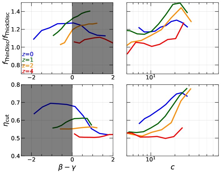
Figure 9: The median mass ratio between thin and thick discs $f_{\rm thin}/f_{\rm thick}$ (upper), and the median circularity threshold $\eta_{\rm cut}$ (lower) as a function of the accretion rate proxy $\beta$-$\gamma$ (left) and halo concentration $c$ (right) at different redshifts. For $f_{\rm thin}/f_{\rm thick}$ and $\eta_{\rm cut}$, we focus on the growing regime ($\beta-\gamma<0$) and environmentally-limited regime ($\beta-\gamma>0$), respectively, where clearer trends can be identified.

In analogy to the analysis of the random-motion supported components, we find that the mass ratio of the two AM-supported components, $f_{\rm thin}/f_{\rm thick}$, as well as the circularity threshold $\eta_{\rm cut}$ used for separating them, also depends on the DM-halo properties. This is shown in Fig. 9. Similar to the subtle distinction between the mass ratio $f_{\rm halo}/f_{\rm bulge}$ and the energy threshold $e_{\rm cut}$, here we reiterate that $\eta_{\rm cut}$ is subtly different from the mass ratio $f_{\rm thin}/f_{\rm thick}$, as it measures how thin (i.e., how coherent in AM) the thin disc is, but not necessarily the mass dominance. $f_{\rm thin}/f_{\rm thick}$ depends on the mass-assembly status of host DM haloes: for a given redshift, the more actively accreting the halo, the less significant the thin disc with respect to the thick one – this can be seen from the regime of $\beta-\gamma<0$, where haloes are still growing. Consistently, the lower the concentration, the less developed the thin disc, since $c$ is generally low for actively accreting systems. Both trends reiterate that the development of a significant thin disc prefers a stable, relaxed halo. Here we refrain from interpreting the complicated behaviors at $\beta-\gamma>0$, where the haloes have been environmentally affected and no longer constitute a clean sample of centrals.

However, for understanding the $\eta_{\rm cut}$ trend, we focus instead on the $\beta-\gamma>0$ regime, as shown in the lower left panel of Fig. 9. At least for the $z=0$ result, the more environmentally affected the host halo, the less coherent the thin disc, as sustained development of a thin disc requires an unperturbed relaxed host. Besides, environmental processes would also contribute to the thickening of discs via encounters with other systems. The redshift trend is in line with this explanation, in the sense that $\eta_{\rm cut}$ is on average lower for higher redshifts, where both accretion and environmental effects are more fierce.

5 Discussion

In this section, we quantify the impact of different decomposition methods on the morphological mass fractions, and address the environmental dependences of $f_{\rm disc}$ and $f_{\rm bulge}$ at different redshifts.

5.1 Comparison with the Zana et al. (2022) method

Our new method inherits the framework of Zana et al. (2022), with the separation of the high-energy and low-energy components basically the same, except for some fine-tuning details accounting for the higher mass resolution of the TNG50 sample. Our key improvement here is the running circularity threshold for thin disc as revealed by the GMM algorithm, as opposed to their constant $\eta_{\rm cut}$ of 0.7. We have demonstrated in Fig. 1 and Figs. 13-16 that this method gives robust identification of thin and thick discs in the circularity-polarity-energy space even when the one-point circularity distribution exhibits no bimodality. Fig. 10 shows the mass fraction of spheroids (halo+bulge) and thin discs at different redshifts, comparing the results from this work and from the method of Zana et al.. First, since our energy criteria are similar, the mass fraction of spheroids are similar. There is a slight difference at $z\leq 2$ and a larger difference at $z=4$ – this is mainly because Zana et al. did not exclude wind particles while we do, and the fraction of wind particles is higher at higher redshifts. The wind particles are short lived and are controlled by hydrodynamics and feedback prescriptions instead of gravitational dynamics, so it is reasonable to exclude them when focusing on the morphology of long-lived stars. This leads to a lower mass fraction of spheroids, more so at higher redshifts when star formation and stellar feedback were more intense.

Second, our new method yields thin discs that are less massive at lower redshift but more massive at higher redshift. This behavior can be anticipated from what is shown in Fig. 2, that most low-$z$ galaxies have $\eta_{\rm cut}>0.7$, except for the low-mass dwarfs of $M_{\star}<10^{8.8}M_{\odot}$, while most high-$z$ galaxies have $\eta_{\rm cut}<0.7$. Similar comparisons could be made for different mass bins or cosmic-web identities, and all lead to the conclusion that the running circularity threshold yields non-monotonic differences with respect to the constant one of 0.7.

5.2 Comparison with Yu et al. (2021) model

Fig. 11 compares the our method to that of Yu et al. (2021, 2023) which uses constant circularity cuts for both bulge and discs. Recall that the Yu et al. method identifies the stellar particles with $\eta<0.2$ as spheroids, and assigns those with $\eta>0.8$ and $0.2<\eta<0.8$ to the thin and thick discs, respectively. This is a representative case of the most commonly used simple kinematic decomposition scheme in the literature (e.g., Genel et al., 2015; Tacchella et al., 2019; Sotillo-Ramos et al., 2023). Their method yields a consistently smaller spheroidal fraction, and under-estimates the mass fraction of thin discs at all redshifts. The offset is particularly strong at high redshift. This highlights the danger of using such simple decomposition schemes for comparing high-$z$ simulations to high-$z$ JWST observations. This again can be understood via Fig. 2, which shows that $\eta_{\rm cut}$ is almost always smaller than 0.8, especially for high-redshift galaxies. Since the simple decomposition scheme underestimates both thin discs and spheroids, the thick disc mass fraction is generally over estimated.

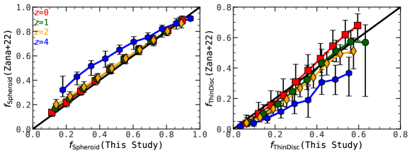
Figure 10: Comparison with the Zana et al. (2022) method, regarding the spheroidal mass fraction (left) and the thin-disc mass fraction (right) at different redshifts. The symbols are the medians with the error bars indicating the 16th and 84th percetiles.

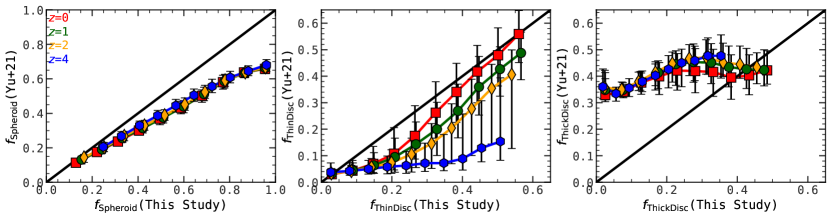
Figure 11: Comparison with the Yu et al. (2021, 2023) method based on constant circularity thresholds, regarding the mass fractions of spheroidal components (left), thin discs (middle), and thick discs (right). The symbols represent the medians, with the error bars indicating the 16th and 84th percetiles. The simple method significantly underestimates thin discs at high-$z$.

5.3 Environment dependence

Above, we have briefly presented the cosmic-web dependence of galaxy morphology whenever there is a trend besides that which can be simply attributed to the mass and redshift dependence of the cosmic-web classification. Here we elaborate on these trends, comparing in Fig. 12 the distributions of disc mass fraction $f_{\rm disc}$ and bulge mass fraction $f_{\rm bulge}$ in different environments at fixed redshifts. First, there is a general behavior across redshifts, that the average bulge fraction decreases towards denser environments while the disc fraction increases from voids to knots. This is particularly clear at intermediate redshifts of $z\sim 1-2$: in knots, the median disc fraction $\langle f_{\rm disc}\rangle$ is higher than the median bulge fraction $\langle f_{\rm bulge}\rangle$, but in voids, $\langle f_{\rm disc}\rangle$ drops to $\sim 0.2$ while $\langle f_{\rm bulge}\rangle$ increases to $\sim 0.6$. At $z=4$, the bulge fraction is always higher than the disc fraction on average, and it is reasonable to speculate that this is the case at even earlier epochs during reionization. This trend is in keeping with the scenario that disc development requires a stable environment, in the sense that central haloes in low-$z$ knots are the most relaxed systems (except for the perturbed backsplash haloes).

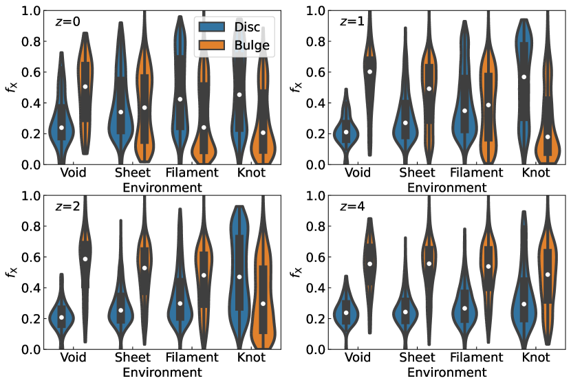
Figure 12: ‘Violin’ plots showing the distributions of the mass-fraction distributions of disc (blue) and bulge (orange) as a function of environment classification, at different redshifts. The white points stand for the median values while the shapes of ‘violin’ stand for the normalized distributions of mass fraction. The central thick bars represent the 25th and 75th percentiles and the thin lines indicate the maximum and minimun values.

Second, the $f_{\rm disc}$ and $f_{\rm bulge}$ distributions are basically unimodal in the least dense environments of voids and sheets, but exhibit bimodality in knots (at $z\la 2$) and filaments (at $z=0$), manifesting the coexistence of disc-dominated and bulge-dominated systems in the denser environments. The distributions are also generally broader in denser environments. Hence, galaxy morphological diversity is affected by environment. The unimodal distributions at the highest redshift suggests that it takes time for environmental effects to accumulate, or that the intense cosmic accretion at early times washed out these effects to some extent. The unimodal $f_{\rm disc}$ distributions in voids is relatively narrow and peak at $f_{\rm disc}\sim 0.2$, indicating that massive discs can hardly develop in isolated environments or at the borders of cosmic knots, this likely manifests limited gas supply in such environments because disc growth requires continuous gas supply in the first place. We have verified that these trends hold if we further keep the halo mass fixed, but opted to show the full sample for better statistics.

6 Conclusions

In this work, we introduce a new morphological decomposition scheme for galaxies in cosmological simulations using stellar kinematics. Similar to Zana et al. (2022), our new decomposition scheme first detects the most prominent local minimum of the energy distribution of star particles and thus breaks a galaxy into higher-energy and lower-energy components – the random-motion supported subsets of which are identified as the stellar halo and the bulge, respectively. It then classifies the remaining rotationally supported stars into two groups in the 3D space spanned by specific energy ($e_{\rm b}$), circularity ($\eta\equiv j_{z}/j_{\rm circ}$), and polarity ($\epsilon\equiv j_{\rm p}/j_{\rm circ}$), using the Gaussian-Mixture-Models algorithm, and identifies the circularity threshold $\eta_{\rm cut}$ for thin and thick discs as the intersection point of the $\eta$ distributions of the two groups.

We have applied this method to the TNG50 simulations and briefly revisited the connection between galaxy morphology and DM halo structure, considering various aspects of halo structure, mass-assembly history (MAH), as well as the location in the cosmic web. We leave more systematic analyses to a future work of this series, but highlight the following take-away messages. Regarding morphological decomposition and morphological fractions, we find that –

• The GMM algorithm reveals a circularity threshold for thin disc ($\eta_{\rm cut}$) that shows galaxy-to-galaxy variance, and systematic variation with halo mass and redshift. The median $\eta_{\rm cut}$ increases with mass from $\simeq 0.5$ at the dwarf regime ($M_{\rm vir}\sim 10^{10}M_{\odot}$) to the peak value of $\simeq 0.8$ at the Milky-Way ($M_{\rm vir}\sim 10^{12}M_{\odot}$) scale, with the exact values slightly higher at lower $z$, and decreases towards higher masses. The energy threshold $e_{\rm cut}$ also exhibits significant halo-to-halo variance and systematic mass and redshift dependence, with the minimum occurring at slightly below the Milky-Way mass ($M_{\rm vir}\sim 10^{11.5}M_{\odot}$). These mass trends can be seen with both stellar mass and halo mass, but are sharpened with halo mass. The characteristic halo mass at which $\eta_{\rm cut}$ peaks or $e_{\rm cut}$ minimizes barely depends on redshift. These all hint at the DM halo playing crucial role in regulating the morphology of inhabitant galaxies, and are in synergy with the theoretical picture generalized from zoom-in cosmological simulations (Dekel et al., 2020a) that gas-rich compaction preludes disc development, and that there is a characteristic halo mass $M_{\rm vir}\sim 10^{11.5}M_{\odot}$ at which the regime transition occurs.

• The constant circularity threshold of $\sim$ 0.7 or 0.8 widely used in the literature (e.g., Yu et al., 2021, 2023; Genel et al., 2015; Tacchella et al., 2019; Sotillo-Ramos et al., 2023) is oversimplified and would result in dramatically biased disc fractions – underestimating thin discs and overestimating thick discs. This is particularly bad at high redshift $z\ga 4$ and thus highlights the danger of using the simplistic decomposition scheme when comparing simulation results with morphological data from the JWST era.

For the structural connections between galaxies and their host haloes, we find that –

• The half-mass size of disc-dominated galaxies, or rather, the compactness of the stellar-disc mass distribution with respect to the virial radius of the host halo, $r_{\rm 1/2}/R_{\rm vir}$, is positively correlated with the DM halo spin parameter $\lambda$ and negatively correlated with halo concentration $c$. The correlation with spin is noticeably stronger than that reported earlier for zoom-in simulations (Jiang et al., 2019), but is weaker than than the linear scaling as in the seminal Mo et al. (1998) model of disc size. The correlation strength is comparable to the high-$z$ results of the THESAN-HR simulation (Shen et al., 2024), which inherits the TNG subgrid physics but adds on-the-fly radiative transfer.

• The concentration dependence of galaxy compactness is similar to that in Jiang et al. (2019), captured roughly by a $c^{-0.7}$ scaling. The concentration dependence is not merely a consequence of the halo contraction in response to the baryonic potential, because it holds even if the concentration is measured from the DM-only simulation for the galaxies with matched counterparts between the full-physics run and the DM-only run.

• The sizes of disc-dominated galaxies depend on redshift such that $r_{\rm 1/2}/R_{\rm vir}$ on average increases from $\sim 0.02$ at $z=0$ to $\sim 0.07$ at $z=4$ or the end of reionization. Newly revealed in this study is that disc compactness also correlates with the mass accretion rate of the DM halo. When halo mass and redshift are fixed, galaxies are more extended in more actively accreting haloes. Specifically, the correlation between $r_{\rm 1/2}/R_{\rm vir}$ and the halo MAH parameter $\beta-\gamma$ is weak but robust across redshifts, with a Pearson correlation coefficient of $\mathcal{R}\simeq-0.2$.

• Besides disc size, the mass ratio between stellar halo and stellar bulge, namely, the ratio between the hotter and colder random-motion supported components, also depend on MAH. More actively accreting haloes tend to have a more significant stellar halo, particularly obvious in cosmic knots. In contrast, the mass ratio between thin and thick discs is lower for the more actively accreting systems, in keeping with the interpretation that disc development needs stable halo conditions.

• The disc mass fraction $f_{\rm disc}$ exhibits positive correlation with the 3D axis ratio $q$ of host halo. With $q$ as an indicator of how relaxed the system is, this reiterates the point that disc development requires stable relaxed haloes. The bulge mass fraction $f_{\rm bulge}$ shows the opposite trend with the halo shape $q$, suggesting that bulge build-up is related to mergers or other processes that disturb the host halo. Both trends are stronger in denser cosmic-web environments.

Overall, with our new GMM-aided morphological decomposition and the exhaustive halo-structure measurements, we conclude that the morphological diversity of galaxies indeed contains useful information about their host halo. These correlations are however complex and in many cases rather weak, posing a challenge to the whole business of quantifying galaxy-halo structural connections. We leave a more detailed study and tentative physical explanations to Paper II, and encourage the community to adapt our methods to other cosmological simulations to further tackle this interesting but challenging issue.

Data Availability

We make our pipeline for morphological decomposition and halo-property measurements publicly available at https://github.com/JinningLianggithub/MorphDecom. The catalogs of TNG50 galaxies with detailed morphological measurements and fittings are available upon reasonable requests and will be available when Paper II is published.

Appendix A Visualization for More Examples

In this Appendix, we show more examples of morphological decomposition for different types of galaxies using method. Fig. 13 shows a massive galaxy at redshift 0 with comparable mass fractions for the four components. Fig. 14 presents a dwarf galaxy. Fig. 15 and Fig. 16 show extreme cases of a disc with marginal stellar halo component and a bulge-dominated system, respectively. These are stress tests though, as we have verified that, with our method, bulgeless pure discs (defined as $f_{\rm disc}>0.9$) are rare, of percent level in TNG50 at $z=0$ and negligible at $z\ga 2$, and the fraction of systems with no stellar halo ($f_{\rm halo}<0.01$) is uniformly rare ($\la 6\%$) across redshifts.

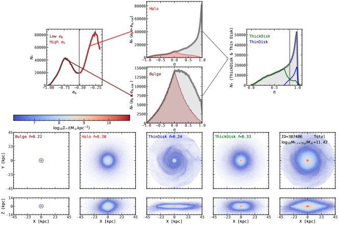
Figure 13: Similar to Figure 1 but for massive galaxy at $z=0$.

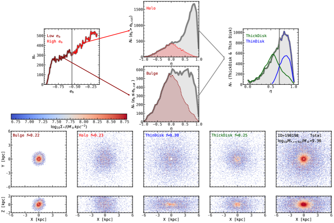
Figure 14: Similar to Figure 1 but for dwarf galaxy at $z=0$.

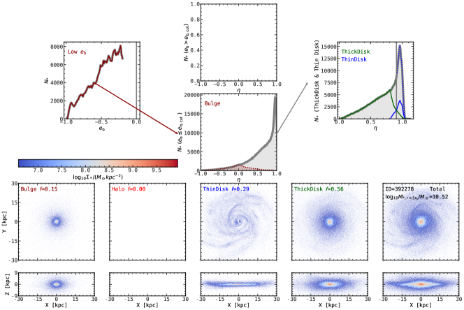
Figure 15: Similar to Figure 1 but for disc-dominated galaxy at $z=0$. Note that in such galaxies, it is possible that there is no energy minima to be found, which leads to this galaxy having no stellar halo

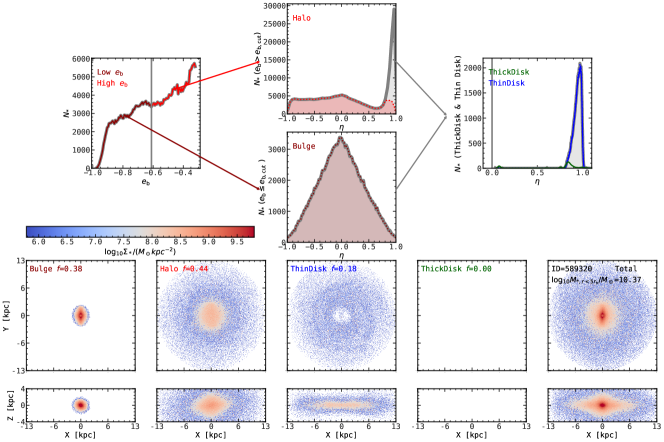
Figure 16: Similar to Figure 1 but for spheroidal-dominated galaxy at $z=0$. Note that in such galaxies, it is possible that there is no circularity threshold to be found, which leads to this galaxy having only one disc (thin disc).

Appendix B Algorithm for detecting the energy threshold

First, we divide the $e_{\rm b}$ distribution into 25 bins ranging from its minimum to the 90th percentile. We then go through each bin $i$ and register all the local minima in the distribution that satisfy the following conditions: (A) $N_{i-1}$ > $N_{i}$ and $N_{i+1}$ $\geq$ $N_{i}$ or $N_{i-1}$ $\geq$ $N_{i}$ and $N_{i+1}$ > $N_{i}$ with $N_{i}$ the number of particles in the $i$-th bin, (B) $N_{i-2}$ > $N_{i}$ and $N_{i+2}$ > $N_{i}$, and (C) $\sum_{j}^{j>i}N_{j}>N_{\rm min}$ where $N_{\rm min}=\text{max}(N_{\rm crit},0.01N_{\star})$, with $N_{\star}$ the total number of bound stellar particles considered and $N_{\rm crit}$ a critical number depending on $N_{\star}$: $N_{\rm crit}=1000$ when $N_{\star}\geq 10^{4}$, $N_{\rm crit}=100$ when $10^{3}\leq N_{\star}<10^{4}$, $N_{\rm crit}=10$ when $N_{\star}\leq 10^{3}$. Zana et al. set $N_{\rm crit}$=1000 for all galaxies irrespective of the mass scale for the TNG100 simulation. Our adaptive scheme yields more robust local minima detection for dwarf galaxies, which are common in the TNG50 box. If no minimum is detected with the three conditions above, the search is extended to the full $e_{\rm b}$ distribution. If there is still no detection, we postulate that there is no high-energy component and thus no stellar halo in this galaxy (and the only random-motion supported component is registered as the stellar bulge). If, instead, multiple minima are detected, we iteratively repeat the search with half the bin size, and require that the distance from the newly detected minima to a previously found one to be smaller than $3\Delta e_{\rm bin}$, with $\Delta e_{\rm bin}$ the bin size at the current iteration step. We stop searching either when a single minimum is left, or when the number of bins reaches a maximum value, which, following Zana et al., is set to be the integer part of $\sqrt{N_{\star}/2}$ in the range between 80 and 400. To avoid the minima which are very close to galactic centres, we require the mass ratio between the lower-energy component and the higher-energy component to be larger than 0.05, and also require $e_{\rm cut}$ candidates to be larger than -0.9. After trimming, if there are still multiple candidates, we adopt the lowest one as $e_{\rm cut}$. To further refine the value of $e_{\rm cut}$ so that it is the $e_{\rm b}$ of a specific stellar particle, we iteratively take the median $e_{\rm b}$ of the stellar particles within the interval centered on the minimum found in the last iteration until the interval width reaches the minimal value corresponding to the maximum number of bins.

Appendix C Gaussian Mixture Model

Mixture models can be used to describe a multi-dimensional distribution $p(\bm{x})$ by combination of $K$ base distributions. In GMM, base distribution is chosen as Gaussian distribution. When the sample data is multivariate, Gaussian distribution function takes form of

$$\mathcal{N}(\bm{x}|\bm{\mu},\bm{\Sigma})=\frac{1}{(2\pi)^{\frac{D}{2}}|\bm{\Sigma}|^{\frac{1}{2}}}\text{exp}\left(-\frac{(\bm{x}-\bm{\mu})^{T}\bm{\Sigma}^{-1}(\bm{x}-\bm{\mu})}{2}\right)$$ (10)

where $\bm{x}$ is data points, $\bm{\mu}$ is the expectation of data, $\bm{\Sigma}$ is the covariance of data and $D$ is the dimension of data.

When we combine a finite number of $K$ Gaussian distribution function to express the distribution function of data, one can get

$$p(\bm{x}|\bm{\theta})=\sum_{k=1}^{K}\pi_{k}\mathcal{N}(\bm{x}|\bm{\mu},\bm{\Sigma})$$ (11)

where $\pi_{k}$ is the $k$th mixture weights which can be treat as the probability of $N(\bm{x}|\bm{\mu},\bm{\Sigma})$ and satisify

$$0\leq\pi_{k}\leq 1,\sum_{k=1}^{K}\pi_{k}=1$$ (12)

where we define $\bm{\theta}=\{\bm{\mu}_{k},\bm{\Sigma}_{k},\bm{\pi}_{k}:k=1,\cdots,K\}$. To get $\bm{\theta}$ with the maximal probability, one needs to do optimization via maximum likelihood.

Unlike a single Gaussian distribution, the likelihood of a mixture model cannot be expressed as closed-form. Therefore, one can only get $\bm{\theta}$ by iteration.

Assume we are given a dataset $\bm{\chi}=\{\bm{x}_{1},\cdots,\bm{x}_{N}\}$, where $\bm{x}_{n}$, $n=1,\cdots,N$ is a sample in this dataset. Log-likelihood can be expressed as

$$\log\left(\bm{\chi}|\bm{\theta}\right)=\sum_{n=1}^{N}\log\sum_{k=1}^{K}\pi_{k}\mathcal{N}(\bm{x}_{n}|\bm{\mu}_{k},\bm{\Sigma}_{k})$$ (13)

One can calculate the parameter $\bm{\theta}$ by the following steps:

1. Initialize $\bm{\mu}_{k}$, $\bm{\Sigma}_{k}$ and $\pi_{k}$

2. Calculate $\mathcal{N}(\bm{x}_{n}|\bm{\mu}_{k},\bm{\Sigma}_{k})$ and $p(\bm{x}|\bm{\theta})$

3. Update $\bm{\mu}_{k}$, $\bm{\Sigma}_{k}$ and $\pi_{k}$

4. Repeat 2 and 3, until the total likelihood $\log\left(\bm{\chi}|\bm{\theta}\right)$ converges or when it reach threshold.

Then one gets $K$ determined Gaussian components to express distribution of data.

Appendix D GMM components in three dimensional space

In Section 3, we use GMM method to separate disky stars into thin and thick disc. The marginal distribution for $\eta$ of two gaussian components can be seen in Fig. 1 and Fig. 13 - Fig. 16. While one can see that the marginal distribution is overlapped, we note that the distribution in three dimensional space, i.e. $\eta$-$\epsilon$-$e_{\rm b}$ space cannot be overlapped. To prove this, we use an dwarf central galaxy (ID 775066) at redshift 0 as an example since smaller number of particles is better for visualization. As one can see in Fig. 17, two gaussian components represented by blue and red points are separated clearly. This indicate that GMM can successfully distinguish two groups.

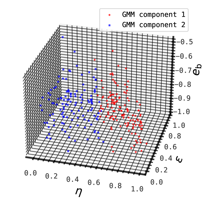
Figure 17: GMM visualization in three dimensional space for disky stars in a dwarf galaxy at redshift 0 (ID 775066). The red circles are GMM component 1, most of which will be identified as a thin disc while blue squares are GMM component 2, most of which will be identified as a thick disc.

References

- Abadi et al. (2003) Abadi M. G., Navarro J. F., Steinmetz M., Eke V. R., 2003, ApJ, 597, 21
- Allgood et al. (2006) Allgood B., Flores R. A., Primack J. R., Kravtsov A. V., Wechsler R. H., Faltenbacher A., Bullock J. S., 2006, MNRAS, 367, 1781
- Behroozi et al. (2013) Behroozi P. S., Wechsler R. H., Conroy C., 2013, ApJ, 770, 57
- Behroozi et al. (2019) Behroozi P., Wechsler R. H., Hearin A. P., Conroy C., 2019, MNRAS, 488, 3143
- Benson (2012) Benson A. J., 2012, New Astronomy, 17, 175
- Blumenthal et al. (1986) Blumenthal G. R., Faber S. M., Flores R., Primack J. R., 1986, ApJ, 301, 27
- Bonamigo et al. (2015) Bonamigo M., Despali G., Limousin M., Angulo R., Giocoli C., Soucail G., 2015, MNRAS, 449, 3171
- Bose et al. (2019) Bose S., Eisenstein D. J., Hernquist L., Pillepich A., Nelson D., Marinacci F., Springel V., Vogelsberger M., 2019, MNRAS, 490, 5693
- Bullock et al. (2001) Bullock J. S., Dekel A., Kolatt T. S., Kravtsov A. V., Klypin A. A., Porciani C., Primack J. R., 2001, ApJ, 555, 240
- Chen et al. (2021) Chen Y., Mo H. J., Li C., Wang K., 2021, Monthly Notices of the Royal Astronomical Society, 504, 4865
- Davis et al. (1985) Davis M., Efstathiou G., Frenk C. S., White S. D. M., 1985, ApJ, 292, 371
- Dekel et al. (2013) Dekel A., Zolotov A., Tweed D., Cacciato M., Ceverino D., Primack J. R., 2013, Monthly Notices of the Royal Astronomical Society, 435, 999
- Dekel et al. (2020a) Dekel A., Ginzburg O., Jiang F., Freundlich J., Lapiner S., Ceverino D., Primack J., 2020a, MNRAS, 493, 4126
- Dekel et al. (2020b) Dekel A., et al., 2020b, MNRAS, 496, 5372
- Doménech-Moral et al. (2012) Doménech-Moral M., Martínez-Serrano F. J., Domínguez-Tenreiro R., Serna A., 2012, MNRAS, 421, 2510
- Du et al. (2019) Du M., Ho L. C., Zhao D., Shi J., Debattista V. P., Hernquist L., Nelson D., 2019, ApJ, 884, 129
- Einasto (1965) Einasto J., 1965, Trudy Astrofizicheskogo Instituta Alma-Ata, 5, 87
- Fall & Efstathiou (1980) Fall S. M., Efstathiou G., 1980, MNRAS, 193, 189
- Forero-Romero et al. (2009) Forero-Romero J. E., Hoffman Y., Gottlöber S., Klypin A., Yepes G., 2009, MNRAS, 396, 1815
- Forero-Romero et al. (2014) Forero-Romero J. E., Contreras S., Padilla N., 2014, MNRAS, 443, 1090
- Freundlich et al. (2020) Freundlich J., et al., 2020, Monthly Notices of the Royal Astronomical Society, 499
- Ganeshaiah Veena et al. (2018) Ganeshaiah Veena P., Cautun M., van de Weygaert R., Tempel E., Jones B. J. T., Rieder S., Frenk C. S., 2018, MNRAS, 481, 414
- Genel et al. (2015) Genel S., Fall S. M., Hernquist L., Vogelsberger M., Snyder G. F., Rodriguez-Gomez V., Sijacki D., Springel V., 2015, ApJ, 804, L40
- Gnedin et al. (2004) Gnedin O. Y., Kravtsov A. V., Klypin A. A., Nagai D., 2004, ApJ, 616, 16
- Hafen et al. (2022) Hafen Z., et al., 2022, MNRAS, 514, 5056
- Hahn et al. (2007) Hahn O., Porciani C., Carollo C. M., Dekel A., 2007, MNRAS, 375, 489
- Hearin et al. (2013) Hearin A. P., Zentner A. R., Berlind A. A., Newman J. A., 2013, MNRAS, 433, 659
- Hopkins et al. (2023) Hopkins P. F., et al., 2023, MNRAS, 525, 2241
- Jiang et al. (2019) Jiang F., et al., 2019, MNRAS, 488, 4801
- Jing & Suto (2002) Jing Y. P., Suto Y., 2002, The Astrophysical Journal, 574, 538
- Kravtsov (2013) Kravtsov A. V., 2013, ApJ, 764, L31
- Lapiner et al. (2023) Lapiner S., et al., 2023, MNRAS, 522, 4515
- Ludlow et al. (2013) Ludlow A. D., et al., 2013, MNRAS, 432, 1103
- Martizzi et al. (2019) Martizzi D., et al., 2019, MNRAS, 486, 3766
- McBride et al. (2009) McBride J., Fakhouri O., Ma C.-P., 2009, MNRAS, 398, 1858
- Menker & Benson (2022) Menker P., Benson A., 2022, MNRAS, 516, 4383
- Mo et al. (1998) Mo H. J., Mao S., White S. D. M., 1998, MNRAS, 295, 319
- Mo et al. (2023) Mo H., Chen Y., Wang H., 2023, arXiv
- Moster et al. (2013) Moster B. P., Naab T., White S. D. M., 2013, MNRAS, 428, 3121
- Navarro et al. (1997) Navarro J. F., Frenk C. S., White S. D. M., 1997, ApJ, 490, 493
- Nelson et al. (2019) Nelson D., et al., 2019, MNRAS, 490, 3234
- Pillepich et al. (2019) Pillepich A., et al., 2019, MNRAS, 490, 3196
- Pontzen & Governato (2013) Pontzen A., Governato F., 2013, MNRAS, 430, 121
- Rodriguez-Gomez et al. (2015) Rodriguez-Gomez V., et al., 2015, MNRAS, 449, 49
- Schneider et al. (2012) Schneider M. D., Frenk C. S., Cole S., 2012, J. Cosmology Astropart. Phys., 2012, 030
- Shen et al. (2024) Shen X., et al., 2024, arXiv e-prints, p. arXiv:2402.08717
- Shi et al. (2015) Shi J., Wang H., Mo H. J., 2015, The Astrophysical Journal, 807, 37
- Somerville et al. (2008) Somerville R. S., Hopkins P. F., Cox T. J., Robertson B. E., Hernquist L., 2008, Monthly Notices of the Royal Astronomical Society, 391, 481
- Somerville et al. (2018) Somerville R. S., et al., 2018, MNRAS, 473, 2714
- Sotillo-Ramos et al. (2023) Sotillo-Ramos D., Bergemann M., Friske J. K. S., Pillepich A., 2023, MNRAS, 525, L105
- Springel et al. (2001) Springel V., White S. D. M., Tormen G., Kauffmann G., 2001, MNRAS, 328, 726
- Tacchella et al. (2019) Tacchella S., et al., 2019, MNRAS, 487, 5416
- Tomassetti et al. (2016) Tomassetti M., et al., 2016, MNRAS, 458, 4477
- Wang et al. (2007) Wang H. Y., Mo H. J., Jing Y. P., 2007, Monthly Notices of the Royal Astronomical Society, 375, 633
- Wang et al. (2011) Wang H., Mo H. J., Jing Y. P., Yang X., Wang Y., 2011, Monthly Notices of the Royal Astronomical Society, 413, 1973
- Wang et al. (2018) Wang H., et al., 2018, The Astrophysical Journal, 852, 31
- White (1984) White S. D. M., 1984, ApJ, 286, 38
- Yang et al. (2003) Yang X., Mo H. J., Bosch V. D., 2003, Monthly Notices of the Royal Astronomical Society, 339, 1057
- Yang et al. (2008) Yang X., Mo H. J., Bosch F. C. v. d., 2008, The Astrophysical Journal, 676, 248
- Yang et al. (2012) Yang X., Mo H. J., Bosch F. C. v. d., Zhang Y., Han J., 2012, The Astrophysical Journal, 752, 41
- Yang et al. (2022) Yang H.-Y., Wang Y., He P., Zhu W., Feng L.-L., 2022, MNRAS, 509, 1036
- Yu et al. (2021) Yu S., et al., 2021, MNRAS, 505, 889
- Yu et al. (2023) Yu S., et al., 2023, MNRAS, 523, 6220
- Zana et al. (2022) Zana T., et al., 2022, MNRAS, 515, 1524
- Zhao et al. (2003) Zhao D. H., Mo H. J., Jing Y. P., Börner G., 2003, Monthly Notices of the Royal Astronomical Society, 339, 12
- Zhao et al. (2009) Zhao D. H., Jing Y. P., Mo H. J., Börner G., 2009, The Astrophysical Journal, 707, 354