GOALS-JWST: The Warm Molecular Outflows of the Merging Starburst Galaxy NGC 3256

Abstract

We present James Webb Space Telescope (JWST) Integral Field Spectrograph observations of NGC 3256, a local infrared-luminous late-stage merging system with two nuclei about 1 kpc apart, both of which have evidence of cold molecular outflows. Using JWST NIRSpec and MIRI datasets, we investigate this morphologically complex system on spatial scales of $<$100 pc, where we focus on the warm molecular H₂ gas surrounding the nuclei. We detect collimated outflowing warm H₂ gas originating from the southern nucleus, though we do not find significant outflowing warm H₂ gas surrounding the northern nucleus. Within the observed region, the maximum intrinsic velocities of the outflow reach up to $\sim$1,000 km s^-1, and extend out to a distance of 0.7 kpc. Based on H₂ S(7)/S(1) line ratios, we find a larger fraction of warmer gas near the S nucleus, which decreases with increasing distance from the nucleus, signifying the S nucleus as a primary source of H₂ heating. The gas mass of the warm H₂ outflow component is estimated to be $M\rm{{}_{warm,out}}$ = 8.9$\times$10${}^{5}\;M_{\odot}$, as much as 4$\%$ of the cold H₂ mass as estimated using ALMA CO data. The outflow time scale is about $7\times 10^{5}$ yr, resulting in a mass outflow rate of $\dot{M}\rm{{}_{warm,out}}$ = 1.3 M_⊙ yr^-1 and kinetic power of $P\rm{{}_{warm,out}}\;\sim\;2\times 10^{41}$ erg s^-1. Lastly, the regions where the outflowing gas reside show high [Fe II]/Pa$\beta$ and H₂/Br$\gamma$ line ratios, indicating enhanced mechanical heating caused by the outflows. At the same time, the 3.3 $\mu$m and 6.2 $\mu$m Polycyclic Aromatic Hydrocarbon fluxes in these regions are not significantly suppressed compared to those outside the outflows, suggesting the outflows have no clear negative feedback effect on the local star formation.

1 Introduction

The physical processes that govern the evolution of galaxies are of fundamental importance to our understanding of how galaxies in the Universe formed. These processes manifest in many forms, including internal mechanisms, such as stellar and AGN outflows (e.g., Müller-Sánchez et al., 2011; U et al., 2019; Aravindan et al., 2023), and external processes such as galaxy mergers (e.g., Lin et al., 2008; Privon et al., 2013; Conselice, 2014). Outflows are believed to regulate and suppress star formation and can, in many instances, lead their hosts to the well-defined red sequence (e.g., Croton et al., 2006; King & Pounds, 2015; Veilleux et al., 2020). Major mergers also play a critical role in the formation of massive galaxies, and are attributed to the co-evolution of the host galaxy and supermassive black holes (e.g., Medling et al., 2015; Ricci et al., 2017; Ramos Almeida et al., 2019) and the formation of compact star clusters (e.g., Mulia et al., 2015; Adamo et al., 2020; Linden et al., 2021). Local luminous infrared galaxies (LIRGs, $L_{\rm IR}>10^{11}L_{\odot}$) are ideal systems for studying these processes because they allow us to analyze evolutionary processes across the full array of merger states, and evaluate the elevated star formation rates triggered by such mergers. Their diversity in starburst and AGN power, merger stages, and outflow activity makes LIRGs compelling ecosystems for tying these properties to the stages of galaxy evolution.

With an infrared luminosity of $L_{\rm IR,\;8-1000\mu m}=3.6\times 10^{11}\;L_{\odot}$ and redshift of $z=0.00936$, NGC 3256 is the most luminous system within $z=0.01$ (Sanders et al., 2003). This system, composed of two gas-rich disk galaxies in a late-stage major merger, is part of the Great Observatories All-sky LIRGs Survey (GOALS; Armus et al., 2009), a sample of bright ($S_{60}>$ 5.24 Jy) LIRGs selected from the IRAS Revised Bright Galaxy Sample (Sanders et al., 2003). The system shows a complex and tidally disturbed morphology, with significantly distorted spiral arms and prominent dust lanes. The two nuclei are in close proximity to each other, $5\farcs 0$ ($\sim$1 kpc), and this system has been extensively observed from X-ray to radio wavelengths (Rich et al., 2011; Piqueras López et al., 2012; Stierwalt et al., 2013; Sakamoto et al., 2014; Ohyama et al., 2015; Chisholm et al., 2016; Harada et al., 2018). These observations have revealed an optically unobscured northern (N) nucleus with signs of starburst activity (Doyon et al., 1994; Boeker et al., 1997; Lira et al., 2002; Lípari et al., 2004; Pereira-Santaella et al., 2011; Laha et al., 2018), while the southern (S) nucleus has been described as a heavily obscured, low-luminosity or nascent AGN (Neff et al., 2003; Sakamoto et al., 2014; Emonts et al., 2014; Ohyama et al., 2015; Michiyama et al., 2018; Yamada et al., 2021).

One of the most compelling aspects of NGC 3256 is the presence of outflows in both nuclei. Submillimeter ALMA observations indicate two different biconical outflows of molecular CO gas originating from the nuclei, with deprojected maximum velocities (and inclination angles) of $\sim$750 (60^∘) and 2600 km s^-1 (20^∘) for the outflows in the northern and southern galaxies, respectively (Sakamoto et al., 2014; Michiyama et al., 2018). Near-infrared (NIR) VLT/SINFONI observations of the S nucleus also reveal biconical outflows in the warm, $>$2000 K H₂ gas, where the gas mass of these outflowing components are estimated to be $\sim$1,200 $M_{\odot}$ (Emonts et al., 2014).

While previous observations have been able to analyze the warm and cold molecular gas phases in NIR and submillimeter wavelengths with great detail, analysis of the warm H₂ component in the mid-infrared (MIR) has been mainly restricted to using the S(1)–S(3) transitions due to the resolution and sensitivity of the Spitzer Space Telescope (e.g. Stierwalt et al., 2013; Inami et al., 2013). Petric et al. (2018) calculated the mass of the warm molecular H₂ component of the northern galaxy to be log($M\rm{{}_{warm}}/\rm{M_{\odot}}$) = 7.38 and a temperature of 322 K within the IRS slits that were centered on the N nucleus. While Spitzer gave a great first look at the warm H₂ gas, the H₂ emission was not spatially resolved and the spectral resolution of Spitzer, R$\sim$60–600, made it difficult to spectrally resolve the outflowing gas in NGC 3256.

The various H₂ transitions and their line ratios with other IR lines are useful for identifying the sources heating the molecular gas and energizing the ISM (Larkin et al., 1998; Riffel et al., 2013; Colina et al., 2015). They can be used to identify the presence of shocks induced by the outflows, and help evaluate the role outflows have in regulating star formation. With JWST, we can now perform the most detailed, spatially resolved analysis of outflowing warm H₂ gas to date in NGC 3256. The unprecedented spatial resolution of JWST enables us to examine the warm H₂ component on scales of $\sim$40–100 pc. We also take advantage of the superb sensitivity and wavelength coverage of JWST to analyze the full set of H₂ 0–0 rotational lines between 5–17 $\mu$m. Specifically, we utilize integral-field spectroscopy (IFS) of the Near-InfraRed Spectrograph (NIRSpec, Böker et al., 2022; Jakobsen et al., 2022) and medium-resolution spectroscopy (MRS) of the Mid-Infrared Instrument (MIRI, Rieke et al., 2015; Labiano et al., 2021; Wright et al., 2023) to assess the kinematics and energetics of the outflows, and evaluate their impact on the local interstellar medium (ISM).

In our analysis, we adopt a cosmology of $H_{0}=70$ km s^-1 Mpc^-1, $\Omega_{\Lambda}=0.72$, and $\Omega_{\rm matter}=0.28$. At the redshift of NGC 3256, $z=0.00936$ (40.4 Mpc), $1\farcs 0$ subtends $\sim$190 pc.

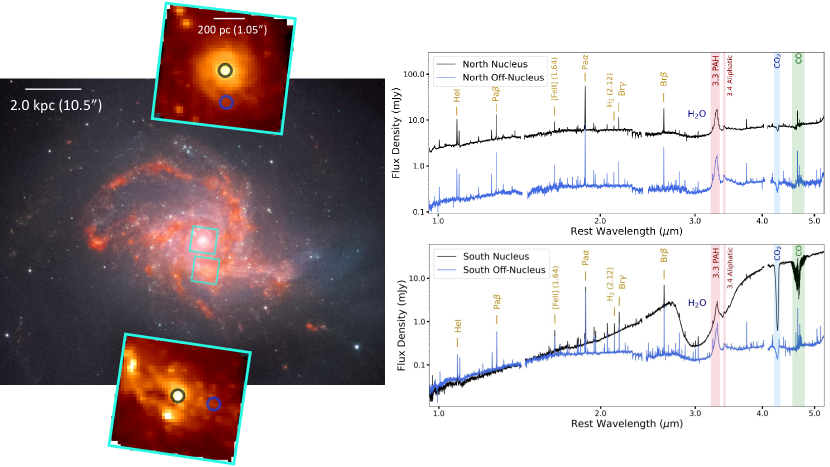
Figure 1: (middle-left) JWST/NIRCam false-color image of NGC 3256 using F150W, F200W, and F444W filters. (top-left, bottom-left) NIRSpec G235H/F170LP 2 $\mu$m continuum images of each nucleus are also shown (field of view size). These images correspond to the locations indicated by the cyan boxes in the NIRCam image. (right) Full NIRSpec spectra (0.97–5.27 $\mu$m) which were extracted from the nuclear (black) and off-nuclear (blue) regions using a $0\farcs 2$ radius aperture (top for the northern nucleus and bottom for the southern nucleus). Their extraction locations and sizes are indicated with the same color in the top-left and bottom-left images, and the spectra shown here were not corrected for aperture losses. The southern nucleus is heavily obscured, significantly redder in the MIR, and has strong 3.05 $\mu$m H₂O and 4.27 $\mu$m CO₂ ice absorption.

2 Observations and Data Reduction

Observations of NGC 3256 were taken as part of the ERS Program 1328 (Co-PIs: L. Armus and A. Evans), for which the JWST/NIRSpec IFS data were taken on 2022 December 23-24 UT. Two sets of observations, each centered on a nucleus, were taken using three high-resolution gratings: G140H/F100LP, G235H/F170LP, and G395H/F290LP. This resulted in a wavelength coverage of 0.97–5.27 $\mu$m, with a nominal resolving power of R$\sim$2700. A 4-point dither pattern was utilized, and total exposure times for all filters were 934 s and 2218 s for the northern and southern pointings, respectively. Observations using JWST/MIRI in the MRS mode were taken on 2022 December 27 UT. Like for NIRSpec, a separate pointing for each nucleus was taken. These observations include all three sub-bands (short [A], medium [B], and long [C]) in all four channels, which cover the full wavelength range from 4.9–28.8 $\mu$m. The total exposure time for each sub-band/channel was 444 s, and was the same for both pointings. In this article, we predominately use channels 1–3, which have a nominal resolving power of R$\sim$2000–3700.

The data were processed through the standard JWST Calibration Pipeline (ver.1.12.5 for NIRSpec; ver.1.11.3 for MIRI, Bushouse et al., 2022). Stage 1 of the reduction pipeline, Detector1, implements detector-level corrections and outputs count-rate data products. Stage 2 (spec2) applies various calibrations steps, including distortion, wavelength, and flux calibrations. Stage 3 (spec3) performs background subtraction for MIRI data and builds the final data cubes from the individual exposures. We also incorporated leakcal calibration in our NIRSpec data. Before stage 3 was implemented, we only included spaxels with data quality (DQ) equal to 0 in order to remove bad spaxels contaminating the NIRSpec data products. We additionally flagged any spaxels in the post-pipeline products with values significantly above emission lines or that were negative.

To properly align both the NIRSpec and MIRI data, Gaia DR3 (Gaia Collaboration et al., 2016, 2023) reference frames of nearby field stars were first used to derive WCS corrections for the JWST/NIRCam and MIRI images (also obtained by ERS 1328, see Linden et al., in prep.). The IFS cubes were subsequently collapsed into a single frame and aligned to the WCS corrected NIRCam/MIRI images, where corrections were around RA: +$0\farcs 02$ and DEC: +$0\farcs 32$ for NIRSpec, and RA: $-0\farcs 01$ and DEC: +$0\farcs 12$ for MIRI.

Lastly, fringing corrections were applied to all MIRI spectra after extraction. We also stitched the spectra by scaling all the continua to that of MIRI channel 3 long, the longest wavelength channel used in our analysis, where scaling factors were typically around 5$\%$.

3 Methods of Analysis

The primary focus of this article is to obtain robust mass estimates and temperatures of the warm outflowing H₂ gas, as well as analyze its kinematics and energetics. Due to the complex kinematic nature of this merging system, robust emission line decompositions and detailed mapping of the spatial structures are needed to accurately identify and study the H₂ gas. To accomplish this, we used the Bayesian AGN Decomposition Analysis for SDSS Spectra (BADASS, Sexton et al., 2021) code. Through Markov-Chain Monte Carlo (MCMC) routines, BADASS performs simultaneous multi-component fits to emission-line spectra. Individual spaxels were fit iteratively across the full spatial extent of the data cubes, where a third order Legendre polynomial was used for the continuum. Emission lines were fit with either Gaussian (recombination, molecular, and fine-structure lines) or Lorentzian functions (Polycyclic Aromatic Hydrocarbon [PAH] features). A secondary Gaussian component to the fit was included based on the F-test of variances: F = $(\sigma\rm{{}_{single}})^{2}/(\sigma\rm{{}_{double}})^{2}$, where $\sigma$ is the standard deviation of the residuals using either a single or double Gaussian fit. If F $>$ 3.0, then adding a second component provided a significant improvement to the fit and was thus justifiable. This secondary component was restricted to have a larger velocity offset from the rest-frame wavelength than the main component. Due to the diverse emission profiles in our data, we left the amplitude and width as unrestricted free parameters. We also set a signal-to-noise (S/N) threshold of 5 for all lines and components to determine a detection. Uncertainties were derived from the error spectrum and the random errors associated with the Bayesian fitting process.

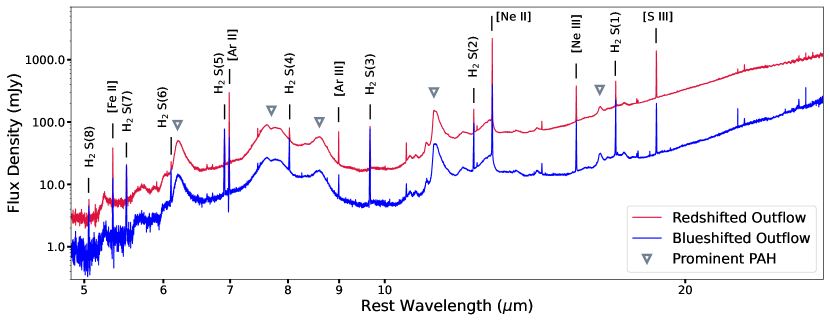
Figure 2: Full MIRI spectra (4.9–27.9 $\mu$m), extracted from the regions where we detect the strongest emission from the secondary (outflow) component seen in all MIRI channels, about 650 and 350 pc to the north and south of the S nucleus (see dotted black circles in Figure 4). An aperture radius of r=$0\farcs 8$ was used, and the spectra have been aperture-corrected but are not corrected for extinction. The rotational H₂ lines used in this study are labeled, along with other MIR emission lines. Prominent PAH features are also marked with upside down triangles. While the emission features of both spectra are similar, the continuum of the blueshifted outflow is about 3–8 times lower than that of the redshited outflow (however, we note that the extraction locations are not equidistant from the nucleus).

4 Results

4.1 Near-Infrared Spectra

In Figure 1, we show images and NIRSpec spectra of the two nuclei and two nearby regions in the disks of NGC 3256. The spectra shown were extracted using an aperture of radius $0\farcs 2$. In the nuclear and off-nuclear regions of both galaxies, we detect a wealth of hydrogen recombination, H₂, He I, and [Fe II] emission lines.

The spectrum of the northern nucleus is similar to that of the off-nuclear regions. They both show a flat continuum and weak H₂O (3.05 $\mu$m) and CO₂ (4.27 $\mu$m) ice absorption. The PAH emission feature at 3.3 $\mu$m is also clearly seen. In contrast, the S nucleus shows a rising MIR continuum and deep H₂O and CO₂ ice absorption. The ice absorption in the S nucleus is significant, with the continuum level dropping by over an order of magnitude. There is also pronounced absorption in the CO rovibrational band at 4.67 $\mu$m (Pereira-Santaella et al., 2024).

Although the NIRSpec observations do not cover the full extent of the CO outflow regions as detected by ALMA (Sakamoto et al., 2014; Michiyama et al., 2018), the regions where there is overlap show blue and red asymmetric profiles in many molecular and ionized emission lines, including [Fe II] 1.25 $\mu$m, H₂ 1.96 $\mu$m, and H₂ 2.12 $\mu$m, that are not seen elsewhere. These blue and red emission wings are detected to within 100 pc of the S nucleus and extend beyond the NIRSpec FoV. In order to study the full extent of the H₂ emission, much of our analysis will focus on the MIRI data, which cover a larger area than NIRSpec.

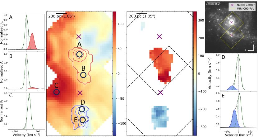
Figure 3: (center) H₂ S(1) 17.0 $\mu$m velocity maps of the main and secondary (outflow) gas components, where the main component is defined as the emission profile closest to the systemic velocity. Flux contours (1.0, 8.0, and 10.0$\times$10^-20 W m^-2) of the H₂ S(1) outflow component are overplotted in red and blue, and the purple crosses are the locations of the nuclei. The full spatial extent of the outflows based on our detection thresholds are plotted in the central-right velocity map (with an adjusted color scale). (upper-right) NIRCam F200W image with the spatial coverage of the velocity map (MIRI channel 3 FoV) is overplotted. (left/right) Aperture extractions (r=$0\farcs 4$) of the normalized S(1) emission at various locations (A - E) are overplotted in the velocity map of the main component and show the diverse emission profiles. The vertical dotted line represents the rest-frame wavelength of S(1). The best-fit model is plotted for each extraction, where the green line represents the main component fit, and the blue and red filled Gaussians represent the blueshifted and redshifted outflow components, respectively. The majority of the outflowing components are spectrally resolved from the main component and show the structure extending to the north and south from the southern nucleus.

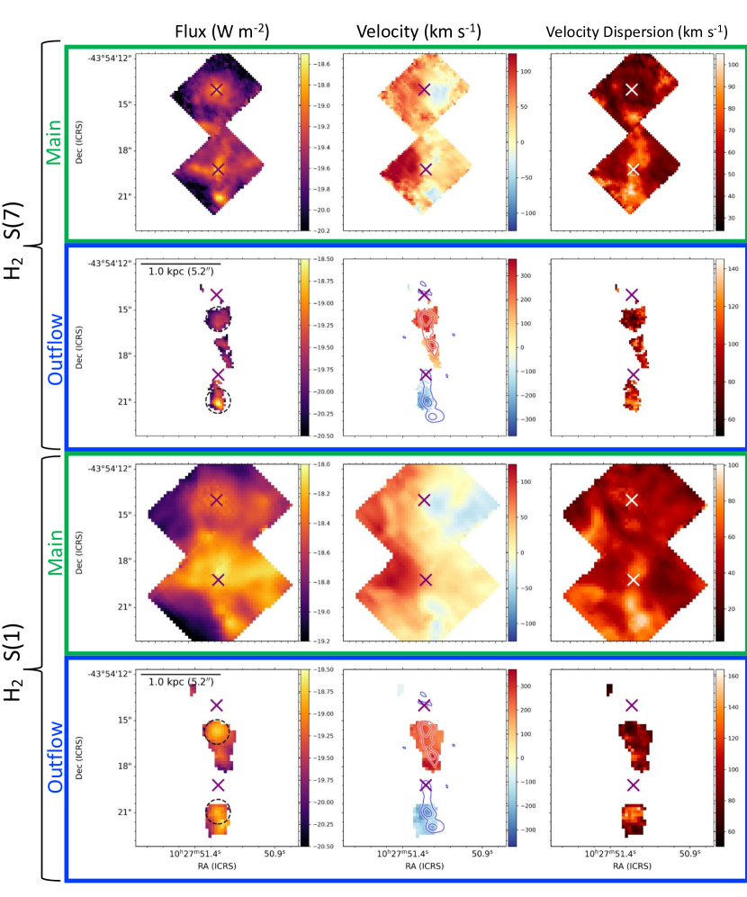
Figure 4: (left to right) Flux, velocity, and dispersion maps of H₂ S(7) (top two rows) and S(1) (bottom two rows) emission lines. Both the main and secondary (outflow) components (see Section 3) are plotted separately. The locations of the nuclei are shown as purple (or white) crosses. The r=$0\farcs 8$ apertures used to extract the 1D spectra plotted Figure 2 and calculate the H₂ gas masses are shown as dotted black circles in the outflow flux panels. ALMA CO flux contours, with velocities set at $\pm$300 km s^-1 (Sakamoto et al., 2014), are overplotted as blue and red contours in the outflow velocity (central) panels. The outflowing warm molecular gas is collimated, extends out to a projected distance of $\sim$600 pc from the S nucleus, and is co-spatial with the cold molecular outflow.

4.2 Warm H₂ Gas

The wavelength coverage of JWST/MIRI allows us to examine the warm H₂ gas using the H₂ 0–0 S(8)–S(1) emission lines from 5.05 to 17.0 $\mu$m. The larger spatial coverage of MIRI (compared to NIRSpec) allows us to better trace the extent of the H₂ emission. In Figure 2, we plot the full MIRI spectra extracted from the regions where we detect the strongest emission observed in all MIRI channels of the secondary, asymmetric H₂ component. These locations are about 650 and 350 pc to the north and south of the S nucleus. The continuum and emission features of both spectra are similar, albeit the continuum level of the redshifted gas is $\sim$3–8 times higher than the blueshifted gas, though this could be due to the different aperture locations relative to the S nucleus.

A sample of the diverse H₂ line profiles in our data are shown in Figure 3, along with the best fit to the main and secondary components, where the main component is defined as the emission profile closest to the systemic velocity. We also plot the velocity maps of the main and secondary H₂ S(1) components in central panels of Figure 3. In the following two subsections, we describe the flux distribution and kinematics of the main and secondary components.

4.2.1 Main H₂ Gas Component

The warm H₂ gas structure of the main component in the northern galaxy appears largely undisturbed while the gas in the southern galaxy appears asymmetric and complex. Specifically, as shown in the first column, first and third rows of Figure 4, there is a horizontal feature, likely the southern galactic disk seen edge-on, that cuts across the S nucleus (English et al., 2003). There is also a vertical structure that reaches a peak luminosity roughly 350 pc south of the S nucleus. In terms of the kinematics, the redshifted emission seen in the northeast extends to the south, where it reaches a maximum velocity of +130 km s^-1 about 300 pc east of the S nucleus (near extraction region C in Figure 3). A similar structure of blueshifted gas to the west of the S nucleus is noticeably absent. Lastly, the velocity dispersion also shows a complex morphology throughout the FoV, and is largest immediately to the north and south of the southern nucleus in the same regions where the secondary component is detected. In contrast, it is comparatively low in the regions surrounding the N nucleus.

4.2.2 Secondary H₂ Gas Component

As shown in Figure 3 and the second and fourth rows of Figure 4, we detect secondary H₂ components that are collimated and symmetric around the S nucleus in the N-S direction. Since these secondary components are spectrally resolved, we define their velocity as the offset of the peak of the component to the peak of the main emission line component. Based on our F-test detection threshold, they are detected out to a projected distance of 650 and 500 pc to the north and south, beyond which their emission is too low to satisfy the F-test. The northward, receding cone grows wider with increasing distance from the S nucleus (closer to the N nucleus), although it appears offset from the S nucleus and there is a noticeable shift eastwards. The spatial structure of southwards, approaching gas appears truncated, particularly in the S(1) emission, however this is likely due to the secondary component falling below our detection threshold (see Section 3). In both the approaching and receding gas, as seen in the velocity maps of Figure 4, the structure of the secondary component is generally co-spatial with the cold CO gas seen in ALMA observations (Sakamoto et al., 2014). At shorter wavelengths (H₂ S(7) 5.5 $\mu$m), the secondary component is detected closer to the southern nucleus, to about 80 pc, which can be seen in the second row of Figure 4.

The kinematics of the secondary component show maximum projected velocities of +350 km s^-1 in the redshifted gas and $-$290 km s^-1 in the blueshifted gas. The velocities appear relatively constant out to the edges of the detected emission, where the emission falls below our detection threshold about 600 pc away from the nucleus. The velocity dispersion is greatest, up to 140 km s^-1, 400 pc south of the S nucleus, and is generally constant ($\sigma\rm{{}_{avg}}$ $\sim$ 90 km s^-1) elsewhere.

4.3 Temperatures and Masses of the Secondary H₂ Gas Component

The extensive wavelength coverage of JWST, combined with its unprecedented sensitivity, allows us to obtain robust gas masses and temperatures of the warm H₂ gas directly from the rotational H₂ lines between 5–17 $\mu$m. Here, we calculate the mass of the secondary H₂ gas component using fluxes and power-law temperature modeling of the different transitions of H₂ (Togi & Smith, 2016). H₂ S(8)–S(1) fluxes were obtained using an aperture of radius $0\farcs 8$ centered on the peak of each of the blueshifted and redshifted secondary components (see dashed circles in Figure 4). This aperture size was chosen to contain as much of the emission as possible, while staying within the FoV of all MIRI channels. Fluxes were aperture and extinction corrected using the Continuum and Feature Extraction (CAFE, Marshall et al., 2007, Díaz-Santos et al.; in prep.) software which uses the 9.7 $\mu$m silicate absorption to estimate the level of extinction. Extinction corrections were generally less than 10$\%$ and were slightly higher in the blueshifted gas. Only the H₂ S(3) line at 9.67 $\mu$m had relatively large corrections, up to 25$\%$.

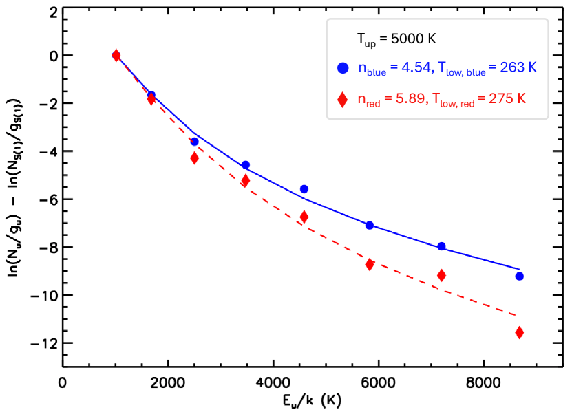
Figure 5: Excitation diagram of the blue and redshifted gas using a r=$0\farcs 8$ aperture centered on the peak flux emission of the secondary (outflow) component. Plotted are the column densities ($N$) of the H₂ S(8)–S(1) transitions, normalized by their statistical weight, $g$, as a function of their energy level $E$. The $N/g$ ratios are normalized with respect to the S(1) transition. The best fits to the red and blueshifted gas are denoted by the dashed red and solid blue lines, respectively. The errors are comparable to the symbol size. The lower power-law index of the blueshifted outflow indicates that it has a larger warm gas mass fraction.

To obtain mass and temperature estimates, we use the power-law model described in Togi & Smith (2016). The power-law index, lower, and upper gas temperatures are the primary model parameters. Since varying the temperature when it is greater than 5000 K has a negligible effect on the quality of the fit and the gas mass, we fixed the upper temperature to 5000 K while the other two parameters were treated as free variables. H₂ line fluxes were used to estimate column densities, whose ratios were then used to create an excitation diagram (see Figure 5). A best-fit model was then fit to the column densities, from which the lower temperature and power-law index were used to calculate the total column density and gas mass.

Fits to the secondary H₂ gas component result in a gas temperature of 263$\pm$19 K and 275$\pm$12 K, and a power law index of 4.54$\pm$0.11 and 5.89$\pm$0.13 for the blueshifted and redshifted gas, respectively. This results in a warm ($>$250 K) molecular gas mass (including a heavy element correction factor of 1.36) of $M\rm{{}_{blue}}$ = (3.5$\pm$0.7)$\times$10${}^{5}\;M_{\odot}$ and $M\rm{{}_{red}}$ = (5.4$\pm$0.9)$\times$10${}^{5}\;M_{\odot}$. Since these apertures do not fully encompass the full extent of the secondary component, the masses calculated here are likely lower limits of the total mass.

To account for the gas mass missed by our apertures, we assumed the power-law indices as calculated from the $0\farcs 8$ extractions are constant throughout the secondary component gas. Since channel 3 has the largest FoV in our analysis and is thus likely to best trace the full extent of the secondary component, we opted to use the two H₂ lines, S(1) and S(2), that are present in this channel. For both S(1) and S(2), we found that the $0\farcs 8$ apertures encompass about 60$\%$ and 65$\%$ of the total detected flux in the blue and redshifted gas, respectively. This implies that the molecular mass could be as high as $M\rm{{}_{blue}}$ = 5.8$\times$10${}^{5}\;M_{\odot}$ and $M\rm{{}_{red}}$ = 8.3$\times$10${}^{5}\;M_{\odot}$. However, these calculations only include the S(8)–S(1) transitions, and not the H₂ S(0) 28.22 $\mu$m line which falls outside the wavelength coverage of our MIRI/MRS data. The inclusion of this line tends to lower the estimated temperature which, in turn, would result in an increase of the calculated gas mass. Because of this, the masses listed above should be considered lower limits.

In addition to large aperture extractions, we can also investigate the temperature distribution of the secondary component on a spaxel-by-spaxel basis. Here, we opt to use the S(1) and S(7) transitions, which are excited at low and high temperatures, respectively. Although S(8) is excited at higher temperatures than S(7), its lower S/N makes it less suited for this analysis.

To compare the S(1) and S(7) maps on the same angular resolution, we first convolved the S(7) flux map (see second row, first panel of Figure 4). The convolution was performed using a Gaussian kernel, which reduced the resolution of the S(7) map (FWHM=$0\farcs 25$) to that of the S(1) map (FHWM=$0\farcs 7$). To account for the difference in pixel size of the two maps, we subsequently rebinned the convolved S(7) map to the larger pixel size of the S(1) map. We then calculated the S(7)/S(1) ratios by dividing the two maps, where pixels with reliable flux measurements in both maps were kept.

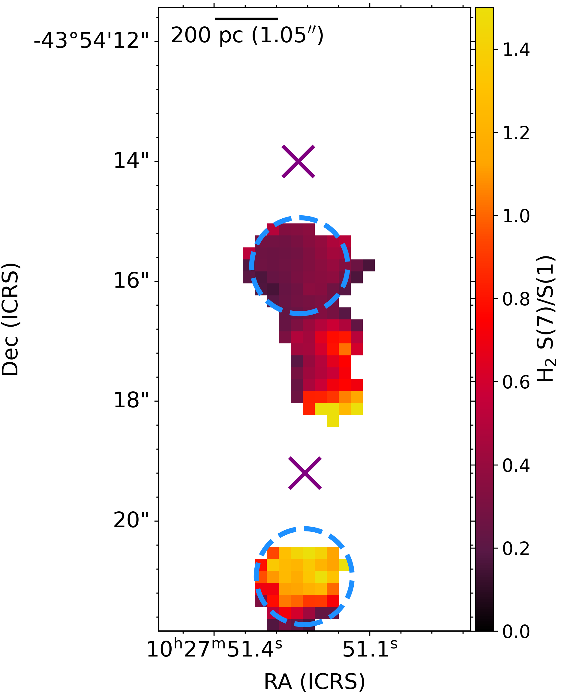
Figure 6: H₂ S(7)/S(1) flux ratio map. The purple crosses indicate the location of the two nuclei, and the apertures used to calculate the mass and power law indices of the secondary component are shown as dashed blue circles. We see higher ratios, indicating a larger fraction of warmer gas, closer to S nucleus, suggesting that the heating of the H₂ is caused by it. We also measure slightly higher average ratios in the southwards, blueshifted gas than the northwards, redshifted gas. Lastly, the temperature distribution within the apertures are indicative of a larger warm gas fraction in blueshifted gas.

The resulting ratio map is shown in Figure 6, where higher line ratios indicate a larger warm gas mass fraction. We find the largest warm gas fractions close to the S nucleus, with the ratios decreasing at larger radii. Our calculated power law indices for the blueshifted and redshifted outflows, 4.54 and 5.89, suggest a higher warm gas fraction in the blueshifted outflow, which is also evident from the temperature distribution. In the redshifted, northwards gas, we measure ratios of $\sim$0.6 at a distance of 300 pc from the S nucleus. This decreases to $\sim$0.3 at 600 pc, where the H₂ fluxes reach their peak in the redshifted gas. For a given distance from the S nucleus, we find slightly higher average ratios in the blueshifted gas, 1.3 at 300 pc, compared to the redshifted gas, 0.6. Unfortunately, we are not able to assess the degree to which the temperature changes beyond 450 pc from the S nucleus, due to the secondary component expanding beyond the MIRI channel 1 FoV.

4.4 Gas Excitation of the ISM

The transitions of H₂, along with ionized hydrogen recombination lines and [Fe II], can be used to analyze the gas excitation of the ISM. H₂ can be excited through thermal processes, such as collisional excitation, as well as non-thermal processes, such as UV (6–13.6 eV) photon absorption. In each case, flux ratios of H₂ lines can be used to help distinguish the different mechanisms (Guillard et al., 2009; Mazzalay et al., 2013; Petric et al., 2018; U et al., 2019). Iron can also serve as a tracer of shocks, since it is mostly embedded in dust grains and released only when these grains are destroyed through thermal sputtering caused by shocks (Storchi-Bergmann et al., 2009; Riffel et al., 2013; Inami et al., 2013). Due to the relative abundance of these lines, trends between H₂/H and [Fe II]/H have been used to help distinguish excitation sources (Larkin et al., 1998; Riffel et al., 2013; Colina et al., 2015; U, 2022; Bianchin et al., 2023).

Figure 7: [Fe II] 1.25 $\mu$m/Pa$\beta$ versus H₂ 1-0 S(1) 2.12 $\mu$m/Br$\gamma$ diagram (left) and associated excitation map of the S nucleus (right). Each spaxel in the full NIRSpec FoV on the right is color-coded based on a linear fit to the line ratios, as shown in the diagram in the left-hand panel. Blue and red contours represent the secondary component (outflows) as traced by the H₂ S(1) 17.0 $\mu$m line (see Figure 4), while the black contour represents the PAH 3.3 $\mu$m emission, set at 1.0, 5.0, and 10.0$\times$10^-19 W m^-2. The white cross at the center marks the location of the S nucleus. The regions where we detect the secondary components (outflows) tend to have higher [Fe II]/Pa$\beta$ and H₂/Br$\gamma$ ratios that are not seen in the regions surrounding the S nucleus.

In the left panel of Figure 7, we explore the spatial variations of gas excitation by investigating the relation between the ratios [Fe II] 1.25 $\mu$m/Pa$\beta$ versus H₂ 1-0 S(1) 2.12 $\mu$m/Br$\gamma$ in the nuclear region of the southern galaxy. Here, line fluxes were calculated from the sum of both the main and secondary components, if present. To show the spatial distribution of the line ratios, we color-code every spaxel in accordance to a linear fit to the ratios, producing an excitation map covering the full NIRSpec FoV, as shown in the right panel of Figure 7. The excitation structure is complex, but there is a noticeable peak in the line ratios to the south of the S nucleus. To the north of the nucleus, there is a broad, high excitation structure that extends westwards. The lowest line ratios are located in the S nucleus and in regions coincident with multiple clumps that are detected in NIRCam imaging (see Linden et al., in prep.). The implications of these regions and corresponding line ratios are discussed in Section 5.3.

5 Discussion

The high velocities and structure of the secondary H₂ emission line component are most consistent with outflowing gas, and we hereafter refer to the secondary component as the outflow component. Although outflowing warm H2 gas has previously been identified (e.g., Emonts et al., 2017; U et al., 2019), this is the first time that the warm H₂ gas in the MIR range is spatially and spectrally resolved.

It is noteworthy, however, that we do not detect a secondary H₂ component in or immediately around the N nucleus. Specifically, our MIR spectra do not show H₂ lines with sufficient asymmetry to pass our detection thresholds (see Section 3) in the regions where the cold molecular outflow from the N nucleus is detected (Sakamoto et al., 2014; Michiyama et al., 2018). As such, for the remainder of this article, we will only reference and analyze the outflows associated with the S nucleus.

5.1 Outflow Characteristics

The symmetry of the outflow structure to the north/south of the S nucleus indicates that it is likely driven by the S nucleus. However, as shown in the spatial maps of Figure 4, we do not detect outflow emission within 80 pc of the nucleus. This is likely because the emission either does not satisfy our S/N $>$ 5 detection threshold, or has a velocity that is too low to be separated from the main gas component. The latter is supported by the higher velocity dispersion in the regions immediately surrounding the nucleus (see right panels of Figure 4), where a spectrally unresolved component could broaden the line profile of the main component, thus making detection of a secondary component more difficult. Additionally, coupled with the fact that the spectral resolution of MIRI is lower for S(1), lower outflow velocities that cannot be spectrally resolved could be a reason why we do not detect S(1) emission as close to the nucleus as S(7). Close inspection of the S(1) line profiles do show faint wings, possibly part of an unresolved component, at similar proximities to the S nucleus as S(7). However, adding a secondary component only marginally improved the fit and did not pass our F-test of variances used for outflow detections. While it is likely that S(1) emission is present closer to the S nucleus, it is difficult to perform robust fits and characterize the outflow parameters within 80 pc.

The outflows are detected out to a distance of 650 and 500 pc (deprojected: 690 and 530 pc) to the north and south of the nucleus. The regions with the highest outflow emission are spatially coincident with strong emission in the main H₂ component and cold CO gas. Moreover, distribution of the HCN and HCO⁺ gas, which trace the denser gas, show enhanced emission in these outflow regions (Michiyama et al., 2018). As such, these H₂ flux peaks could be caused by the outflowing gas impacting a dense region in the ISM.

The kinematics of the outflows show maximum projected velocities to be +350 km s^-1 to the north and $-$290 km s^-1 to the south. To obtain intrinsic velocities, we adopt the outflow inclination as calculated by Sakamoto et al. (2014) and Emonts et al. (2014), $i_{\rm{out}}\sim 20^{\circ}$. Deprojecting the outflows, v_out/sin$(i_{\rm{out}})$, we obtain maximum intrinsic velocities of +1020 and $-$850 km s^-1, respectively (where v_out,avg= 750 km s^-1, averaged across all regions of the outflows).

Inspection of the outflow spatial maps (Figure 4) shows that the northwards (redshifted) outflow appears to have a marginal eastward shift as it expands outwards. Based on the relative location of the two galaxies and the interlaced nature of their disks (see NIRCam imaging in Figure 1), this shift eastwards could be induced by the disk rotation of the northern galaxy. If the northern disk is rotating clockwise (Sakamoto et al., 2014), then this could potentially shift the outflowing gas eastward, explaining the angled structure relative to the S nucleus.

5.2 Outflow Mass Comparisons of MIR to NIR and Submillimeter Measurements

In Section 4.3, we calculated the mass of the warm outflowing gas to be $M\rm{{}_{blue,out}}$ = (3.5$\pm$0.7)$\times$10${}^{5}\;M_{\odot}$ and $M\rm{{}_{red,out}}$ = (5.4$\pm$0.9)$\times$10${}^{5}\;M_{\odot}$ for the blueshifted and redshifted outflows in the emission peak regions. We can compare these masses to that of the hotter ($\sim$2000 K) gas observed at NIR wavelengths. To measure this hotter component, we use the H₂ 1-0 S(1) 2.12 $\mu$m outflow flux map created by Emonts et al. (2014), which was derived from K-band VLT/SINFONI observations (program ID: 078.B-0066(A), PI: Luis Colina). Measuring the flux within the same apertures used to calculate the warm MIR gas mass and following the methods described in Mazzalay et al. (2013) and Emonts et al. (2014), we obtain mass measurements of 330$\pm$60 and 200$\pm$35 $M_{\odot}$ for the blue and redshifted outflows, respectively. This combined gas mass of 530 $M_{\odot}$ is almost 2$\times$10³ times lower than the warm MIR component, (8.9$\pm$1.1)$\times$10${}^{5}\;M_{\odot}$.

In order to assess the contribution of the warm gas to the total multiphase component, we can use molecular CO to estimate the mass of the outflowing cold H₂ gas. To do this, we opted to use archival CO (2-1) ALMA data (project code: 2015.1.00902.S, PI: Yiping Ao), which has higher spatial resolution than the CO (1-0) map of Sakamoto et al. (2014). Using the same two r=$0\farcs 8$ apertures used in our H₂ mass calculations, we extracted spectra of the CO (2-1) emission. Based on a two-component Gaussian fit, we measured line fluxes of 20.6$\pm$2.1 and 8.6$\pm$1.9 Jy km s^-1 with velocity offsets of $-$150 km s^-1 and $+$250 km s^-1 for the blueshifted and redshifted gas, respectively. These are consistent with the mean velocities measured in the warm H₂ outflow, $-$170 km s^-1 and $+$240 km s^-1. Following Michiyama et al. (2018), we set L_CO(2-1)/L_CO(1-0) as unity. For the CO to H₂ conversion factor, $\alpha\rm{{}_{CO}}$=$M\rm{{}_{mol}}$$/L\rm{{}_{CO}}$, we assume a value of 0.8 $M_{\odot}$ (K km s^-1 pc²)^-1, which is typically used for ULIRGs (Downes & Solomon, 1998; Bryant & Scoville, 1999). This value is 5.4 times lower than the galactic value of 4.32. This is because ULIRGs, particularly those involved in mergers, typically have increased CO linewidths (and thus greater L_CO) caused by the heightened turbulence and temperatures induced by the outflows and mergers. From these assumptions, we obtained $M\rm{{}_{blue,out}}$ = (1.6$\pm$0.2)$\times$10${}^{7}\;M_{\odot}$ and $M\rm{{}_{red,out}}$ = (6.8$\pm$1.5)$\times$10${}^{6}\;M_{\odot}$, which implies the combined outflowing mass is $M\rm{{}_{cold,out}}$ = (2.3$\pm$0.3)$\times$10${}^{7}\;M_{\odot}$.

While we assumed a value of 0.8 for $\alpha\rm{{}_{CO}}$, Cicone et al. (2018) calculated $\alpha\rm{{}_{CO}}$ to be 2.1 where molecular outflows are present. This in turn would increase our cold gas mass estimate to $M\rm{{}_{cold,out}}$ = (6.0$\pm$0.8)$\times$10${}^{7}\;M_{\odot}$. More recently, Pereira-Santaella et al. (2024) estimated $\alpha\rm{{}_{CO}}$ of various regions around the outflows in NGC 3256 utilizing the CO rovibrational band at 4.67 $\mu$m. From their two-component model, they report $\alpha\rm{{}_{CO}}$ to be 0.62. Setting $\alpha\rm{{}_{CO}}$ as 0.62 reduces our combined cold gas mass to (1.8$\pm$0.3)$\times$10${}^{7}\;M_{\odot}$, still consistent with the mass calculated using the canonical conversion factor for local ULIRGs. Hereafter, we adopt 2.3$\times$10${}^{7}\;M_{\odot}$ for the reminder of our analysis.

Combining the redshifted and blueshifted outflows, the $M\rm{{}_{warm}}$/$M\rm{{}_{cold}}$ gas mass fraction is about 4$\%$. As mentioned previously, we note that our data set does not include the S(0) 28.22 $\mu$m line which tends to lower the estimated temperature, thus increasing the $M\rm{{}_{warm}}$/$M\rm{{}_{cold}}$ fraction. Higdon et al. (2006) measured typical warm gas mass fractions in observed ULIRGs to be slightly less than 1$\%$ (as calculated from the S(1) 17.0 $\mu$m to S(3) 9.67 $\mu$m line fluxes). However, they found that the inclusion of S(0) could increase $M\rm{{}_{warm}}$/$M\rm{{}_{cold}}$ to tens of percent. While the warm mass fraction may depend heavily on the inclusion of S(0), our estimates for the warm mass fraction in the outflows are comparable to those measured in other local active galaxies (Rigopoulou et al., 2002).

In Section 5.1, we calculated the maximum intrinsic outflow velocity to be $\sim$10³ km s^-1, and maximum deprojected distance to be 700 pc. Following this, the outflow time scale, $t\rm{{}_{out}}$, is estimated to be $7\times 10^{5}$ yr. Assuming a conical geometry, this results in a time-averaged outflow mass rate of $\dot{M}\rm{{}_{warm,out}}$ = 1.3 M_⊙ yr^-1. If a significant portion of the outflow mass is in the cold component, then the outflow mass rate could be as high as $\dot{M}\rm{{}_{cold,out}}$ = 33 M_⊙ yr^-1, which is slightly lower than the 48 M_⊙ yr^-1 reported by Sakamoto et al. (2014). Regardless, these values are comparable to rates seen in other Seyferts and ULIRGs (García-Burillo et al., 2014; Cicone et al., 2014). These rates, particularly the cold gas mass rate, are high compared to estimates of the star formation rate (SFR). In regions around the S nucleus, Emonts et al. (2014) and Michiyama et al. (2018) estimated the SFR to be 1 - 6.8 M_⊙ yr^-1 based on hydrogen recombination line calibrations. For the cold molecular outflow, this leads to a mass loading factor, $\dot{M}\rm{{}_{out}}$/SFR, of 5 or greater. Amongst starburst galaxies, mass loading factors are typically around unity while AGN-dominated sources tend to be higher ($>3$) (Cicone et al., 2014).

5.3 Gas Conditions in the Outflow

To investigate the impact the outflows have on the local ISM, we plot [Fe II]/Pa$\beta$ versus H₂/Br$\gamma$ line ratios in Figure 7. Higher [Fe II] and H₂ line ratios relative to the recombination lines indicate stronger gas excitation, and are located at the southern edge of the FoV, where they are spatially coincident with the blueshifted outflow. This region is also where the outflow flux is the strongest (see Figure 4) and has the highest fraction of warm gas (see Figure 6). This increase in the H₂ and [Fe II] line ratios could be caused by the outflow impacting a denser region in the ISM, possibly in an interaction with the disk of the northern galaxy. This interpretation can be supported by the comparatively low value of the power-law index of the southern outflow, 4.54, which is lower than the mean found in other galaxies, 4.84 (Togi & Smith, 2016). Indices in this range are seen in other cases where shocks are present (Appleton et al., 2017), suggesting a shock front created by the outflow. However, most of the outflow falls outside the NIRSpec FoV, so it is difficult to assess the full effect of the excitation using this method. While the narrow FoV limits us from analyzing the redshifted outflow as well, the outflow regions that do fall within the NIRSpec FoV of the north galaxy also show elevated values for these line ratios, indicating that the northwards outflow may also be energizing the ISM.

5.4 Outflow Energetics and Feedback

5.4.1 Energy of the Outflow

To explore the energy source of the outflows, we can calculate the combined kinetic energy of the outflows by combining turbulent and bulk components,

$$E{\rm{{}_{kin}}}=E{\rm{{}_{turb}}}+E{\rm{{}_{bulk}}}=\frac{3}{2}M\sigma^{2}+\frac{1}{2}Mv\rm{{}_{out}}^{2}$$ (1)

Setting $M=M\rm{{}_{warm,out}}=8.9\times 10^{5}\;M_{\odot}$, $\sigma\rm{{}_{avg}}$ $\sim$ 90 km s^-1, and $v\rm{{}_{out,avg}}\;\sim$ 750 km s^-1 gives a combined outflow energy of $E\rm{{}_{warm,kin}}\;\sim\;5\times 10^{54}$ erg. For the cold H₂ outflow, where $M\rm{{}_{cold,out}}\;2.3\times 10^{7}\;M_{\odot}$, and assuming the same kinematics yields $E\rm{{}_{cold,kin}}\;\sim\;1\times 10^{56}$ erg. Assuming the outflow time scale to be $7\times 10^{5}$ yr, this results in a kinetic power of $P\rm{{}_{warm,out}}\;\sim\;2\times 10^{41}$ erg s^-1 and $P\rm{{}_{cold,out}}\;\sim\;6\times 10^{42}$ erg s^-1.

Put together, the temperatures, kinematics, and energetics of the outflows can provide clues to their origin. As shown in Figure 6, we find the highest warm gas fractions close to the S nucleus, with fractions decreasing at larger radii, an indication of heating from the nuclear source. Moreover, in addition to the symmetry to the north and south of the S nucleus, the fast velocities ($\sim$10³ km s^-1), large mass loading factor ($>5$), and power ($6\times 10^{42}$ erg s^-1) found here are all typical of AGN-driven outflows (Rodríguez-Ardila et al., 2006; Müller-Sánchez et al., 2011; Hill & Zakamska, 2014; Bae & Woo, 2016; Harrison et al., 2016; Veilleux et al., 2020).

5.4.2 Feedback on Star Formation

It is well known that sustained outflows can suppress star formation (e.g., King & Pounds, 2015; Armus et al., 2020). A commonly used IR tracer of star formation are PAHs (Peeters et al., 2004; Inami et al., 2018; Lai et al., 2020, 2022). Because PAH grains are fragile, they can easily be destroyed in harsh radiation environments. As such, we can utilize PAH fluxes to assess if the outflows have any significant feedback on the local ISM. For this, we opt to use the 3.3 and 6.2 $\mu$m PAHs since they are isolated from other features and offer the best spatial resolution among the PAHs available in JWST.

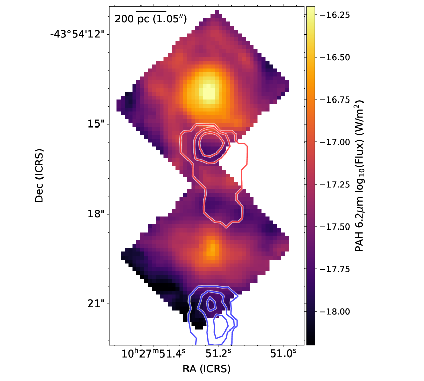
Figure 8: PAH 6.2 $\mu$m flux map, plotted over the full MIRI channel 1 FoV. Blue and red contours mark the regions where we detect the molecular outflows, as traced by H₂ S(1) 17.0 $\mu$m emission. The PAH emission is strongest in the nuclear region of each galaxy, with prominent emission also seen in the disks and spiral arms. There is no clear indication that the PAH emission is being suppressed by the outflows.

In the right panel of Figure 7, we plot 3.3 $\mu$m PAH flux contours over the excitation map. Most of the PAH flux is centered around the S nucleus with emission extending to the east and west, likely tracing the disk of the southern galaxy. The emission seems to decrease in the outflow regions but the limited FoV makes it difficult to ascertain the exact correlation between the outflow and PAH emission. As such, we can take advantage of a larger FoV of MIRI to examine the PAH at 6.2 $\mu$m, as shown in the flux map of Figure 8. Like PAH 3.3 $\mu$m, we measure the strongest PAH emission at the nuclear region of each galaxy, with other prominent emission seen in the disks and spiral arms, likely caused by the star formation occurring there. As was done in Figure 4, we overlay the outflowing gas as traced by the H₂ S(1) 17.0 $\mu$m. While the PAH emission is generally lower in the regions coincident with the outflow, we see no clear disruption in the overall PAH structure. The PAH emission clearly traces the disks and spiral arms, and regions with lower emission are likely due to the geometry of the system. Although the outflows we detect are fast and significantly heat the molecular gas, we do not see any clear evidence of them inducing negative feedback on the local star formation.

6 Conclusion

Utilizing the exceptional resolution and sensitivity of JWST, we investigate the nearby merging LIRG NGC 3256 on scales of $<$100 pc. Here, we showcase the capability of JWST to spatially resolve the MIR H₂ lines, allowing us to directly identify and trace the outflowing warm H₂ gas. Using the H₂ lines from 5.0–17.0 $\mu$m, we analyze the mass, temperature distribution, kinematics, and energetics of the outflowing warm H₂ gas, and assess the impact of the outflows on the local star formation. The following is a summary of our findings:

•  Warm, outflowing H₂ gas is detected in a collimated outflow originating from the southern nucleus. The outflows extend out to a distance of 700 pc, and have a deprojected maximum velocity of $\sim$1,000 km s^-1. The emission is most intense near the far edges of the outflows, possibly due to impacting the disk of the northern galaxy. We do not detect any significant outflowing H₂ gas originating from the northern nucleus.

•  Using the extensive wavelength coverage of JWST, we use the full set of S(8)–S(1) H₂ lines to directly calculate the outflowing warm H₂ gas mass: $M\rm{{}_{warm,out}}$ = 8.9$\times$10${}^{5}\;M_{\odot}$, where the $M\rm{{}_{warm}}$/$M\rm{{}_{cold}}$ mass fraction is 4$\%$. With an outflow time scale of about $7\times 10^{5}$ yr, the outflow mass rate is about $\dot{M}\rm{{}_{warm,out}}$ = 1.3 M_⊙ yr^-1. These masses yield an outflow energy of $E\rm{{}_{warm}}\;\sim\;5\times 10^{54}$ erg and kinetic power of $P\rm{{}_{warm,out}}\;\sim\;2\times 10^{41}$ erg s^-1. The mass loading factor of the warm outflowing gas is roughly unity. However, when taking into account the cold H₂ component, it could 5 or higher.

•  The spatial map of the outflowing H₂ S(7)/S(1) flux ratio reveals higher ratios closer to the S nucleus. This indicates a larger fraction of warmer gas is closer to the nucleus and decreases as the outflow expands outwards, suggesting that the S nucleus is the heating source of the outflowing gas.

•  Analysis of the gas excitation in the outflow regions using [Fe II]/Pa$\beta$ and H₂/Br$\gamma$ line ratios shows enhanced ratios compared to those seen in typical star forming regions, indicating the outflow is energizing these regions, possibly as a shock. The value of the power-law index is also indicative of shocks, particularly in the blueshifted outflow. However, flux maps of the 6.2 $\mu$m PAH do not show the outflowing gas having a clear negative feedback effect on the local star formation.

In this article, we have showcased the unique capabilities of JWST that enable us to explore the warm molecular gas in the MIR with both superb spectral and spatial resolutions. Further observations of other warm molecular outflows in the MIR and direct comparisons to the cold dense gas and the ionized atomic gas on similar physical scales will allow for a comprehensive study of the the multi-phase outflows in nearby star forming galaxies and AGN.

The JWST data presented in this paper were obtained from the Mikulski Archive for Space Telescopes (MAST) at the Space Telescope Science Institute, which is operated by the Association of Universities for Research in Astronomy, Inc., under NASA contract NAS 5-03127 for JWST. These observations are associated with program 1328 and are supported by NASA grant ERS-01328. They can be accessed at 10.17909/8mkr-xr82 (catalog https://doi.org/10.17909/8mkr-xr82). STScI is operated by the Association of Universities for Research in Astronomy, Inc., under NASA contract NAS5–26555. Support to MAST for these data is provided by the NASA Office of Space Science via grant NAG5–7584 and by other grants and contracts. T.B. and H.I. acknowledge support from JSPS KAKENHI Grant Number JP21H01129 and the Ito Foundation for Promotion of Science. A.S.E. and S.T.L. acknowledge support from NASA grants HST-GO15472 and HST-GO16914. V.U. acknowledges partial funding support from NASA Astrophysics Data Analysis Program (ADAP) grant Nos. 80NSSC20K0450 and 80NSSC23K0750 and STScI grant Nos. HST-AR-17063.005-A, HST-GO-17285.001-A, and JWST-GO-01717.001-A. C.R. acknowledges support from Fondecyt Regular grant 1230345 and ANID BASAL project FB210003 The Flatiron Institute is supported by the Simons Foundation. S.A. gratefully acknowledges support from an ERC Advanced Grant 789410, the Swedish Research Council and the Knut and Alice Wallenberg (KAW) foundation. F.M-S. acknowledges support from NASA through ADAP award 80NSSC19K1096. This paper makes use of the following ALMA data: ADS/JAO.ALMA$\#$2011.0.00525.S and 2015.1.00902.S. ALMA is a partnership of ESO (representing its member states), NSF (USA) and NINS (Japan), together with NRC (Canada), NSTC and ASIAA (Taiwan), and KASI (Republic of Korea), in cooperation with the Republic of Chile. The Joint ALMA Observatory is operated by ESO, AUI/NRAO and NAOJ.

References

- Adamo et al. (2020) Adamo, A., Hollyhead, K., Messa, M., et al. 2020, MNRAS, 499, 3267, doi: 10.1093/mnras/staa2380
- Appleton et al. (2017) Appleton, P. N., Guillard, P., Togi, A., et al. 2017, ApJ, 836, 76, doi: 10.3847/1538-4357/836/1/76
- Aravindan et al. (2023) Aravindan, A., Liu, W., Canalizo, G., et al. 2023, ApJ, 950, 33, doi: 10.3847/1538-4357/acca7c
- Armus et al. (2020) Armus, L., Charmandaris, V., & Soifer, B. T. 2020, Nature Astronomy, 4, 467, doi: 10.1038/s41550-020-1106-3
- Armus et al. (2009) Armus, L., Mazzarella, J. M., Evans, A. S., et al. 2009, PASP, 121, 559, doi: 10.1086/600092
- Astropy Collaboration et al. (2013) Astropy Collaboration, Robitaille, T. P., Tollerud, E. J., et al. 2013, A&A, 558, A33, doi: 10.1051/0004-6361/201322068
- Astropy Collaboration et al. (2018) Astropy Collaboration, Price-Whelan, A. M., Sipőcz, B. M., et al. 2018, AJ, 156, 123, doi: 10.3847/1538-3881/aabc4f
- Astropy Collaboration et al. (2022) Astropy Collaboration, Price-Whelan, A. M., Lim, P. L., et al. 2022, ApJ, 935, 167, doi: 10.3847/1538-4357/ac7c74
- Bae & Woo (2016) Bae, H.-J., & Woo, J.-H. 2016, ApJ, 828, 97, doi: 10.3847/0004-637X/828/2/97
- Bianchin et al. (2023) Bianchin, M., U, V., Song, Y., et al. 2023, arXiv e-prints, arXiv:2308.00209, doi: 10.48550/arXiv.2308.00209
- Boeker et al. (1997) Boeker, T., Storey, J. W. V., Krabbe, A., & Lehmann, T. 1997, PASP, 109, 827, doi: 10.1086/133951
- Böker et al. (2022) Böker, T., Arribas, S., Lützgendorf, N., et al. 2022, A&A, 661, A82, doi: 10.1051/0004-6361/202142589
- Bryant & Scoville (1999) Bryant, P. M., & Scoville, N. Z. 1999, AJ, 117, 2632, doi: 10.1086/300879
- Bushouse et al. (2022) Bushouse, H., Eisenhamer, J., Dencheva, N., et al. 2022, spacetelescope/jwst: JWST 1.6.2, 1.6.2, Zenodo, Zenodo, doi: 10.5281/zenodo.6984366
- Chisholm et al. (2016) Chisholm, J., Tremonti, C. A., Leitherer, C., Chen, Y., & Wofford, A. 2016, MNRAS, 457, 3133, doi: 10.1093/mnras/stw178
- Cicone et al. (2014) Cicone, C., Maiolino, R., Sturm, E., et al. 2014, A&A, 562, A21, doi: 10.1051/0004-6361/201322464
- Cicone et al. (2018) Cicone, C., Severgnini, P., Papadopoulos, P. P., et al. 2018, ApJ, 863, 143, doi: 10.3847/1538-4357/aad32a
- Colina et al. (2015) Colina, L., Piqueras López, J., Arribas, S., et al. 2015, A&A, 578, A48, doi: 10.1051/0004-6361/201425567
- Conselice (2014) Conselice, C. J. 2014, ARA&A, 52, 291, doi: 10.1146/annurev-astro-081913-040037
- Croton et al. (2006) Croton, D. J., Springel, V., White, S. D. M., et al. 2006, MNRAS, 365, 11, doi: 10.1111/j.1365-2966.2005.09675.x
- Downes & Solomon (1998) Downes, D., & Solomon, P. M. 1998, ApJ, 507, 615, doi: 10.1086/306339
- Doyon et al. (1994) Doyon, R., Joseph, R. D., & Wright, G. S. 1994, ApJ, 421, 101, doi: 10.1086/173629
- Emonts et al. (2017) Emonts, B. H. C., Colina, L., Piqueras-López, J., et al. 2017, A&A, 607, A116, doi: 10.1051/0004-6361/201731508
- Emonts et al. (2014) Emonts, B. H. C., Piqueras-López, J., Colina, L., et al. 2014, A&A, 572, A40, doi: 10.1051/0004-6361/201423805
- English et al. (2003) English, J., Norris, R. P., Freeman, K. C., & Booth, R. S. 2003, AJ, 125, 1134, doi: 10.1086/367914
- Gaia Collaboration et al. (2016) Gaia Collaboration, Prusti, T., de Bruijne, J. H. J., et al. 2016, A&A, 595, A1, doi: 10.1051/0004-6361/201629272
- Gaia Collaboration et al. (2023) Gaia Collaboration, Vallenari, A., Brown, A. G. A., et al. 2023, A&A, 674, A1, doi: 10.1051/0004-6361/202243940
- García-Burillo et al. (2014) García-Burillo, S., Combes, F., Usero, A., et al. 2014, A&A, 567, A125, doi: 10.1051/0004-6361/201423843
- Guillard et al. (2009) Guillard, P., Boulanger, F., Pineau Des Forêts, G., & Appleton, P. N. 2009, A&A, 502, 515, doi: 10.1051/0004-6361/200811263
- Harada et al. (2018) Harada, N., Sakamoto, K., Martín, S., et al. 2018, ApJ, 855, 49, doi: 10.3847/1538-4357/aaaa70
- Harrison et al. (2016) Harrison, C. M., Alexander, D. M., Mullaney, J. R., et al. 2016, MNRAS, 456, 1195, doi: 10.1093/mnras/stv2727
- Higdon et al. (2006) Higdon, S. J. U., Armus, L., Higdon, J. L., Soifer, B. T., & Spoon, H. W. W. 2006, ApJ, 648, 323, doi: 10.1086/505701
- Hill & Zakamska (2014) Hill, M. J., & Zakamska, N. L. 2014, MNRAS, 439, 2701, doi: 10.1093/mnras/stu123
- Inami et al. (2013) Inami, H., Armus, L., Charmandaris, V., et al. 2013, ApJ, 777, 156, doi: 10.1088/0004-637X/777/2/156
- Inami et al. (2018) Inami, H., Armus, L., Matsuhara, H., et al. 2018, A&A, 617, A130, doi: 10.1051/0004-6361/201833053
- Jakobsen et al. (2022) Jakobsen, P., Ferruit, P., Alves de Oliveira, C., et al. 2022, A&A, 661, A80, doi: 10.1051/0004-6361/202142663
- King & Pounds (2015) King, A., & Pounds, K. 2015, ARA&A, 53, 115, doi: 10.1146/annurev-astro-082214-122316
- Labiano et al. (2021) Labiano, A., Argyriou, I., Álvarez-Márquez, J., et al. 2021, A&A, 656, A57, doi: 10.1051/0004-6361/202140614
- Laha et al. (2018) Laha, S., Guainazzi, M., Piconcelli, E., et al. 2018, ApJ, 868, 10, doi: 10.3847/1538-4357/aae390
- Lai et al. (2020) Lai, T. S. Y., Smith, J. D. T., Baba, S., Spoon, H. W. W., & Imanishi, M. 2020, ApJ, 905, 55, doi: 10.3847/1538-4357/abc002
- Lai et al. (2022) Lai, T. S. Y., Armus, L., U, V., et al. 2022, ApJ, 941, L36, doi: 10.3847/2041-8213/ac9ebf
- Larkin et al. (1998) Larkin, J. E., Armus, L., Knop, R. A., Soifer, B. T., & Matthews, K. 1998, ApJS, 114, 59, doi: 10.1086/313063
- Lin et al. (2008) Lin, L., Patton, D. R., Koo, D. C., et al. 2008, ApJ, 681, 232, doi: 10.1086/587928
- Linden et al. (2021) Linden, S. T., Evans, A. S., Larson, K., et al. 2021, ApJ, 923, 278, doi: 10.3847/1538-4357/ac2892
- Lípari et al. (2004) Lípari, S. L., Díaz, R. J., Forte, J. C., et al. 2004, MNRAS, 354, L1, doi: 10.1111/j.1365-2966.2004.08213.x
- Lira et al. (2002) Lira, P., Ward, M., Zezas, A., Alonso-Herrero, A., & Ueno, S. 2002, MNRAS, 330, 259, doi: 10.1046/j.1365-8711.2002.05014.x
- Marshall et al. (2007) Marshall, J. A., Herter, T. L., Armus, L., et al. 2007, ApJ, 670, 129, doi: 10.1086/521588
- Mazzalay et al. (2013) Mazzalay, X., Saglia, R. P., Erwin, P., et al. 2013, MNRAS, 428, 2389, doi: 10.1093/mnras/sts204
- Medling et al. (2015) Medling, A. M., U, V., Max, C. E., et al. 2015, ApJ, 803, 61, doi: 10.1088/0004-637X/803/2/61
- Michiyama et al. (2018) Michiyama, T., Iono, D., Sliwa, K., et al. 2018, ApJ, 868, 95, doi: 10.3847/1538-4357/aae82a
- Mulia et al. (2015) Mulia, A. J., Chandar, R., & Whitmore, B. C. 2015, ApJ, 805, 99, doi: 10.1088/0004-637X/805/2/99
- Müller-Sánchez et al. (2011) Müller-Sánchez, F., Prieto, M. A., Hicks, E. K. S., et al. 2011, ApJ, 739, 69, doi: 10.1088/0004-637X/739/2/69
- Neff et al. (2003) Neff, S. G., Ulvestad, J. S., & Campion, S. D. 2003, ApJ, 599, 1043, doi: 10.1086/379596
- Ohyama et al. (2015) Ohyama, Y., Terashima, Y., & Sakamoto, K. 2015, ApJ, 805, 162, doi: 10.1088/0004-637X/805/2/162
- Peeters et al. (2004) Peeters, E., Spoon, H. W. W., & Tielens, A. G. G. M. 2004, ApJ, 613, 986, doi: 10.1086/423237
- Pereira-Santaella et al. (2024) Pereira-Santaella, M., González-Alfonso, E., García-Bernete, I., García-Burillo, S., & Rigopoulou, D. 2024, A&A, 681, A117, doi: 10.1051/0004-6361/202347942
- Pereira-Santaella et al. (2011) Pereira-Santaella, M., Alonso-Herrero, A., Santos-Lleo, M., et al. 2011, A&A, 535, A93, doi: 10.1051/0004-6361/201117420
- Petric et al. (2018) Petric, A. O., Armus, L., Flagey, N., et al. 2018, AJ, 156, 295, doi: 10.3847/1538-3881/aaca35
- Piqueras López et al. (2012) Piqueras López, J., Colina, L., Arribas, S., Alonso-Herrero, A., & Bedregal, A. G. 2012, A&A, 546, A64, doi: 10.1051/0004-6361/201219372
- Privon et al. (2013) Privon, G. C., Barnes, J. E., Evans, A. S., et al. 2013, ApJ, 771, 120, doi: 10.1088/0004-637X/771/2/120
- Ramos Almeida et al. (2019) Ramos Almeida, C., Acosta-Pulido, J. A., Tadhunter, C. N., et al. 2019, MNRAS, 487, L18, doi: 10.1093/mnrasl/slz072
- Ricci et al. (2017) Ricci, C., Bauer, F. E., Treister, E., et al. 2017, MNRAS, 468, 1273, doi: 10.1093/mnras/stx173
- Rich et al. (2011) Rich, J. A., Kewley, L. J., & Dopita, M. A. 2011, ApJ, 734, 87, doi: 10.1088/0004-637X/734/2/87
- Rieke et al. (2015) Rieke, G. H., Ressler, M. E., Morrison, J. E., et al. 2015, PASP, 127, 665, doi: 10.1086/682257
- Riffel et al. (2013) Riffel, R., Rodríguez-Ardila, A., Aleman, I., et al. 2013, MNRAS, 430, 2002, doi: 10.1093/mnras/stt026
- Rigopoulou et al. (2002) Rigopoulou, D., Kunze, D., Lutz, D., Genzel, R., & Moorwood, A. F. M. 2002, A&A, 389, 374, doi: 10.1051/0004-6361:20020607
- Rodríguez-Ardila et al. (2006) Rodríguez-Ardila, A., Prieto, M. A., Viegas, S., & Gruenwald, R. 2006, ApJ, 653, 1098, doi: 10.1086/508864
- Sakamoto et al. (2014) Sakamoto, K., Aalto, S., Combes, F., Evans, A., & Peck, A. 2014, ApJ, 797, 90, doi: 10.1088/0004-637X/797/2/90
- Sanders et al. (2003) Sanders, D. B., Mazzarella, J. M., Kim, D. C., Surace, J. A., & Soifer, B. T. 2003, AJ, 126, 1607, doi: 10.1086/376841
- Sexton et al. (2021) Sexton, R. O., Matzko, W., Darden, N., Canalizo, G., & Gorjian, V. 2021, MNRAS, 500, 2871, doi: 10.1093/mnras/staa3278
- Stierwalt et al. (2013) Stierwalt, S., Armus, L., Surace, J. A., et al. 2013, ApJS, 206, 1, doi: 10.1088/0067-0049/206/1/1
- Storchi-Bergmann et al. (2009) Storchi-Bergmann, T., McGregor, P. J., Riffel, R. A., et al. 2009, MNRAS, 394, 1148, doi: 10.1111/j.1365-2966.2009.14388.x
- Togi & Smith (2016) Togi, A., & Smith, J. D. T. 2016, ApJ, 830, 18, doi: 10.3847/0004-637X/830/1/18
- U (2022) U, V. 2022, Universe, 8, 392, doi: 10.3390/universe8080392
- U et al. (2019) U, V., Medling, A. M., Inami, H., et al. 2019, ApJ, 871, 166, doi: 10.3847/1538-4357/aaf1c2
- Veilleux et al. (2020) Veilleux, S., Maiolino, R., Bolatto, A. D., & Aalto, S. 2020, A&A Rev., 28, 2, doi: 10.1007/s00159-019-0121-9
- Wright et al. (2023) Wright, G. S., Rieke, G. H., Glasse, A., et al. 2023, PASP, 135, 048003, doi: 10.1088/1538-3873/acbe66
- Yamada et al. (2021) Yamada, S., Ueda, Y., Tanimoto, A., et al. 2021, ApJS, 257, 61, doi: 10.3847/1538-4365/ac17f5