Abstract

In this paper we present a new antithetic multilevel Monte Carlo (MLMC) method for the estimation of expectations with respect to laws of diffusion processes that can be elliptic or hypo-elliptic. In particular, we consider the case where one has to resort to time discretization of the diffusion and numerical simulation of such schemes. Motivated by recent developments, we introduce a new MLMC estimator of expectations, which does not require simulation of intractable Lévy areas but has a weak error of order 2 and achieves the optimal computational complexity. We then show how this approach can be used in the context of the filtering problem associated to partially observed diffusions with discrete time observations. We illustrate with numerical simulations that our new approaches provide efficiency gains for several problems relative to some existing methods.
Keywords: Filtering, hypo-elliptic diffusion, multilevel Monte Carlo, stochastic differential equations.

1 Introduction

We consider the following $N$-dimensional stochastic differential equation (SDE):

$$dX_{t}=\sigma_{0}(X_{t})dt+\sum_{1\leq j\leq d}\sigma_{j}(X_{t})dB_{t}^{j},\quad X_{0}=x\in\mathbb{R}^{N},$$ (1)

where $\{B_{t}\}_{t\geq 0}$ is the $d$-dimensional standard Brownian motion defined upon the filtered probability space $(\Omega,\mathcal{F},\{\mathcal{F}_{t}\}_{t\geq 0},\mathbb{P})$, and $\sigma_{j}:\mathbb{R}^{N}\to\mathbb{R}^{N}$ satisfies some regularity conditions, to be made precise later, with $\sigma_{j}=[\sigma_{j}^{1},\ldots,\sigma_{j}^{N}]^{\top}$ for $0\leq j\leq d$. Throughout the paper, the matrix $a=\sigma\sigma^{\top}$ can be degenerate, with $\sigma\equiv[\sigma_{1},\ldots,\sigma_{d}]$. Thus, this class of diffusion process includes certain elliptic and hypo-elliptic diffusion processes that can be found in applications; see for instance [24]. In particular, a lot of interest has been shown recently in the literature for numerical analysis and statistical inference methods for hypo-elliptic diffusions (see e.g. [6, 12, 16, 15]). We consider the context that one cannot obtain an exact solution of this SDE, despite its existence, and has to resort to time-discretization of the diffusion and the associated numerical simulation and, again, there are many examples of such processes that are used in practice [24].

The collection of problems that we focus upon in this article is, firstly, the computation of expectations with respect to (w.r.t.) laws of diffusion processes; we call this the forward problem. That is, given a function $\varphi:\mathbb{R}^{N}\rightarrow\mathbb{R}$ that is integrable w.r.t. the transition law of the diffusion, the objective is the computation of a numerical approximation of $\mathbb{E}[\varphi(X_{T})]$ for some given terminal time $T>0$. This has numerous applications, e.g. option pricing in mathematical finance [11]. Secondly, we consider the filtering problem for partially observed diffusion processes that are discretely observed in time. In other words (1) is a latent process that is observed through noisy data, only at discrete times (which we take as unit times for simplicity). The objective is then to compute an approximation of the conditional expectation of $X_{t}$ at each observation time and given all the data available up-to that time. This is a classical problem in engineering, statistics and applied mathematics, see e.g. [2, 4] for further references and applications. Our numerical methods will ultimately rely on (stochastic) Monte Carlo simulation, to be detailed later on.

For both afore-mentioned problems, one must resort to a time discretization of (1) whose properties can be critical for any resulting numerical approximation method relying on it. There are several numerical methods in the literature, such as the Euler-Maruyama (E-M) method and the Milstein scheme; see for instance [24]. The main properties that are often of interest to inform the efficiency of the approximation are the weak and strong error, which we shall define, loosely, as follows – a full definition can be found later on. For a time discretization on a regular grid of spacing $\Delta>0$, and a corresponding numerical approximation $\{\bar{X}_{t}\}_{t\geq 0}$ the weak error (assuming it exists) is:

$$|\mathbb{E}[\varphi(X_{T})]-\mathbb{E}[\varphi(\bar{X}_{T})]|$$

for an appropriate test function $\varphi:\mathbb{R}^{N}\to\mathbb{R}$. We remark that the numerical approximation may be defined in continuous time by interpolation between points on the time grid. The strong error (assuming it exists) is taken as:

$$\mathbb{E}\bigl{[}\|X_{T}-\bar{X}_{T}\|^{2}\bigr{]}$$

where $\|\cdot\|$ is the $L_{2}-$norm. There are several results for well-known discretization methods; e.g., E-M has weak error of $\mathcal{O}(\Delta)$ (weak error 1) and strong error of $\mathcal{O}(\Delta)$ (strong error 1) and the Milstein scheme has weak error 1 and strong error 2. In the context of the methods to be used in this article, one generally would like both the weak and strong error to be ‘large’ at a cost of $\mathcal{O}(\Delta^{-1})$ for directly simulating the approximation. We note that direct simulation, without for instance solving linear equations of cost of order $\mathcal{O}(N^{m})$, $m>2$, is critical for practical problems, especially filtering.

In this work we consider both elliptic and hypo-elliptic diffusion processes and in the latter case we often have $N\geq 2$. In such scenarios, the Milstein method (or the strong 1.5 scheme, see [24], with weak error 2 and strong error 3) cannot often be simulated directly, without a restrictive commutative condition (given later on), as one has to compute an intractable Lévy area. This means that in such cases one resorts to the E-M approach, which can be simulated exactly, but whose weak and strong errors are comparatively low. Whilst there are some higher order discretization methods based upon stochastic Runge-Kutta approaches (see e.g. [28]), generally for many Monte Carlo simulation-based methods a strong error of 2 generally suffices for ‘optimal’ (to be clarified later on) variance properties. An elegant methodology that side-steps sampling of Lévy areas but preserves the strong order of approximation was developed in [10] based upon the multilevel Monte Carlo (MLMC) approach [8, 9, 13].

MLMC works with a hierarchy of time-discretised diffusions, that is with a collection of step-sizes $0<\Delta_{0}<\cdots<\Delta_{L}$, $L\in\mathbb{N}$. Then one rewrites the expectation of interest as a decomposition of the difference of the exact (no time discretization) expectation and the one with the finest time discretization and then a telescoping sum of differences of expectations associated to increasingly coarse step-sizes. Then, if one can appropiately simulate dependent (coupled) time discretizations for pairs of step-sizes it is possible to reduce the cost of a Monte Carlo based algorithm (e.g. the cost versus a direct simulation of the time discretised diffusion with a single step-size $\Delta_{L}$) to achieve a pre-specified mean square error (MSE) using MLMC; see e.g. [9] for a review. [10] introduce an antithetic MLMC (AMLMC) using the truncated Milstein scheme (defined in Section 2.2.2) which has weak error 1 and stong error 1, but the AMLMC still provides an optimal computational complexity without requiring the simulation of intractable Lévy areas.

In this article we develop a new method (multilevel-based) for time discretization which is effective in both the elliptic and hypo-elliptic contexts. Motivated by the work in [10], we derive a new AMLMC based on the numerical scheme proposed in [15] achieving weak error 2 and strong error 1 (the latter is proven in this article), which still gives an optimal computational complexity (for the forward problem). The method can also be simulated directly with a cost of $\mathcal{O}(\Delta^{-1})$ per-pair of levels $0<\Delta<\Delta^{\prime}$. An AMLMC with a weak error 2 has also been investigated in [1], where they used an alternative numerical scheme with a weak error 2 and emphasized its efficiency due to the reduction of the number of time-discretizations, which is an advantage over the AMLMC that uses the truncated Milstein scheme (weak error 1). A comparison between our proposed AMLMC and the method by [1] is given later in Section 2.4. In addition, we show that our new methodology can be used for the filtering problem. Some of the state-of-the-art numerical methods for this problem are based upon particle filters (e.g. [4, 5]) related to the MLMC approach, which are termed multilevel particle filters (MLPFs) see e.g. [17, 23]. Based upon the methodology developed herein, we derive a new MLPF.

To summarize, the main contributions of this article are:

• We introduce a locally non-degenerate scheme of weak error 2 for both elliptic/hypo-elliptic contexts, inspired by [15]. We prove that the scheme has strong error 1.

• Based on the above scheme, we develop a new AMLMC method for elliptic and hypo-elliptic SDEs that does not contain Lévy areas and prove that the variance of the AMLMC estimator decays (w.r.t the step-size) at the same rate as for a discretization scheme that would achieve a strong error 2.

• We show that for the important class of small-noise diffusions, i.e. SDEs containing a parameter $\mu\ll 1$ at the front of the diffusion coefficient, the variance of the proposed AMLMC estimator vanishes as $\mathcal{O}(\mu^{2})$ – in constrast with the antithetic scheme of [10] when the corresponding variances do not diminish for small $\mu$.

• We show how to use the new AMLMC method for filtering within the context of MLPFs.

• We illustrate our approaches in several numerical examples for both the forward and filtering problems. We show numerically that our method can out-perform some competing appraches.

We further elaborate on some of the bullet points above. In the case of the forward problem, the second bullet point leads to the new AMLMC estimator having a cost of $\mathcal{O}(\epsilon^{-2})$ to give a MSE of $\mathcal{O}(\epsilon^{2})$, $\epsilon>0$, i.e. the method attains the optimal cost for (stochastic) Monte Carlo based methods. Such a MSE is also achieved by [10], however our superior weak error is expected to provide efficiency gains – verified in our numerical experiments – due to the nessecity of the use of a finite $L$ (the most precise level) in simulations. Furthermore, the third bullet implies that our new AMLMC method achieves diminishing variance for small-noise diffusions (many models in applications are within this scope), which also prompts reduction of the computational cost. In the case of filtering, we compare to the MLPF approaches in [17, 23], which either provably or in simulations (the proofs, when obtained, were only for the elliptic case) achieve a MSE of $\mathcal{O}(\epsilon^{2})$ for a cost of $\mathcal{O}(\epsilon^{-2.5})$ and $\mathcal{O}(\epsilon^{-2}\log(\epsilon)^{2})$ respectively; note that the MLPF method of [23] corresponds to an embedding of the multilevel approach of [10] within the filtering problem. We verify in our simulations that, as one expects based upon [17], our new MLPF has costs consistent with the anticipated rate $\mathcal{O}(\epsilon^{-2}\log(\epsilon)^{2})$ to achieve a MSE of $\mathcal{O}(\epsilon^{2})$. However, as the discretization schemes underpinning the methods in [17, 23] have weak error 1, we again observe efficiency gains for finite $L$. Finally, we note that our numerical scheme is locally non-degenerate under a hypo-elliptic setting, while this is not the case for the truncated Milstein scheme. The existence of the density (non-degeneracy) is important in the filtering problem when utilising guided proposals to improve the performance of particle filters.

This paper is structured as follows. In Section 2 we consider several numerical schemes for SDEs and introduce our approach. In Section 3 we describe how our idea can be used in the context of the filtering problem and derive the new MLPF. In Section 4 we present our numerical results which help to illustrate our theoretical results. The mathematical proofs of our main results are given in Appendix.

Notation: Let $C_{b}^{K}(\mathbb{R}^{n};\mathbb{R}^{m})$, $n,m,K\in\mathbb{N}$, be the space of $K$-times differentiable functions $f:\mathbb{R}^{n}\to\mathbb{R}^{m}$ such that partial derivatives up to order $K$ are bounded. For a vector $y\in\mathbb{R}^{N}$, we define a norm $\|\cdot\|$ as $\|y\|\equiv\sqrt{\sum_{1\leq i\leq N}y_{i}^{2}}$.

2 Numerical Schemes

2.1 Basic Assumptions and Error

To study a broad class of SDEs including the case where the matrix $a=\sigma\sigma^{\top}$ is degenerate, we consider the following structure for model (1):

$$dX_{t}=\begin{bmatrix}dX_{S,t}\\ dX_{R,t}\end{bmatrix}=\begin{bmatrix}\sigma_{S,0}(X_{t})\\[2.84544pt] \sigma_{R,0}(X_{t})\end{bmatrix}dt+\sum_{1\leq j\leq d}\begin{bmatrix}\mathbf{0}_{N_{S}}\\[2.84544pt] \sigma_{R,j}(X_{t})\end{bmatrix}dB_{t}^{j},\qquad X_{0}=x\in\mathbb{R}^{N},$$ (2)

where we have set $\sigma_{S,0}:\mathbb{R}^{N}\to\mathbb{R}^{N_{S}},\,\sigma_{R,j}:\mathbb{R}^{N}\to\mathbb{R}^{N_{R}},\,0\leq j\leq d,$ with integers $N_{S}\geq 0$, $N_{R}\geq 1$ such that $N_{S}+N_{R}=N$. We write for $x\in\mathbb{R}^{N}$,

$$\sigma_{0}(x)=\begin{bmatrix}\sigma_{S,0}(x)\\[2.84544pt] \sigma_{R,0}(x)\end{bmatrix},\qquad\sigma_{j}(x)=\begin{bmatrix}\mathbf{0}_{N_{S}}\\[2.84544pt] \sigma_{R,j}(x)\end{bmatrix},\quad 1\leq j\leq d,$$

and $a\equiv\sigma\sigma^{\top}$ with $\sigma\equiv[\sigma_{1},\ldots,\sigma_{d}]$. Notice that when $N_{S}\geq 1$, the matrix $a$ is degenerate. We write:

$$[\sigma_{0},\sigma_{j}](x)=\sum_{1\leq k\leq N}\bigl{\{}\widetilde{\sigma}_{0}^{k}(x)\partial_{x_{k}}\sigma_{j}(x)-{\sigma}_{j}^{k}(x)\partial_{x_{k}}\widetilde{\sigma}_{0}(x)\bigr{\}},\qquad 1\leq j\leq d,$$

where $\widetilde{\sigma}_{0}:\mathbb{R}^{N}\to\mathbb{R}^{N}$ is the drift function when (2) is written as the Stratonovich-type SDE.

We introduce the following assumptions realted to Hörmander’s condition (see e.g. [27]):

Assumption 2.1.

$\sigma_{j}\in C_{b}^{\infty}(\mathbb{R}^{N};\mathbb{R}^{N})$, $0\leq j\leq d$.

Assumption 2.2.

(i) Ellipticity. When $N_{S}=0$, it holds that for any $x\in\mathbb{R}^{N}$:

$$\mathrm{Span}\bigl{\{}\sigma_{1}(x),\ldots,\sigma_{d}(x)\bigr{\}}=\mathbb{R}^{N},$$

which is equivalent to the matrix $a(x)=\sigma(x)\sigma(x)^{\top}$ being positive definite for any $x\in\mathbb{R}^{N}$.
(ii) Hypo-ellipticity. When $N_{S}\geq 1$, it holds that for any $x\in\mathbb{R}^{N}$:

$$\mathrm{Span}\bigl{\{}\sigma_{R,1}(x),\ldots,\sigma_{R,d}(x)\bigr{\}}=\mathbb{R}^{N_{R}};$$

$$\mathrm{Span}\bigl{\{}\sigma_{1}(x),\ldots,\sigma_{d}(x),[\sigma_{0},\sigma_{1}](x),\ldots,[\sigma_{0},\sigma_{d}](x)\bigr{\}}=\mathbb{R}^{N}.$$

For a numerical scheme $\{\bar{X}_{k\Delta}\}_{k=0,1,\ldots,2^{\ell}}$ with constant step-size $\Delta=T/2^{\ell}$ and non-negative integer $\ell$, a weak and strong error of order $m\geq 1$ are each defined as follows, for any $p\geq 1$:

$$\left|\mathbb{E}\left[\varphi(X_{T})\right]-\mathbb{E}\left[\varphi(\bar{X}_{T})\right]\right|=\mathcal{O}(\Delta^{m}),\qquad\mathbb{E}\Bigl{[}\max_{0\leq k\leq 2^{\ell}}\bigl{\|}X_{k\Delta}-\bar{X}_{k\Delta}\bigr{\|}^{2p}\Bigr{]}=\mathcal{O}(\Delta^{mp}),$$

for some appropriate test function $\varphi:\mathbb{R}^{N}\to\mathbb{R}$.

2.2 Discretizations

We introduce a discretization scheme of weak order 2 which will have a key involvement in our methodology. We also mention other popular discretization schemes (e.g. Milstein scheme) for comparison. Let $T>0$ be a terminal time and $\Delta_{\ell}=T/2^{\ell}$ be a step-size of discretization with a non-negative integer $\ell$. We make use of the notation $t_{k}=k\Delta_{\ell}$, $1\leq k\leq 2^{\ell}$, and $\Delta B_{t,s}=B_{t}-B_{s},\,0<s<t$. For a sufficiently smooth function $\varphi:\mathbb{R}^{N}\to\mathbb{R}$, we set:

$$\mathscr{L}_{0}\varphi(x) =\sum_{1\leq k\leq N}\sigma_{0}^{k}(x)\partial_{x_{k}}\varphi(x)+\tfrac{1}{2}\sum_{1\leq j\leq d}\sum_{1\leq k_{1},k_{2}\leq N}\sigma_{j}^{k_{1}}(x)\sigma_{j}^{k_{2}}(x)\partial_{x_{k_{1}}}\partial_{x_{k_{2}}}\varphi(x);$$

$$\mathscr{L}_{i}\varphi(x) =\sum_{1\leq k\leq N}\sigma_{i}^{k}(x)\partial_{x_{k}}\varphi(x),\qquad 1\leq i\leq d.$$

We define, for $1\leq i_{1},i_{2}\leq d$,

$$[\sigma_{i_{1}},\sigma_{i_{2}}](x)=\mathscr{L}_{i_{1}}\sigma_{i_{2}}(x)-\mathscr{L}_{i_{2}}\sigma_{i_{1}}(x),\qquad x\in\mathbb{R}^{N},$$

where $\mathscr{L}_{i_{1}}\sigma_{i_{2}}(x)=[\mathscr{L}_{i_{1}}\sigma_{i_{2}}^{1}(x),\ldots,\mathscr{L}_{i_{1}}\sigma_{i_{2}}^{N}(x)]^{\top}\in\mathbb{R}^{N}.$

2.2.1 Milstein scheme

The Milstein scheme, of weak order 1 and strong order 2, writes as:

$$\bar{X}_{t_{k+1}}^{\mathrm{Mil}}=\bar{X}_{t_{k}}^{\mathrm{Mil}}+\sigma_{0}(\bar{X}_{t_{k}}^{\mathrm{Mil}})\Delta_{\ell}+\sum_{1\leq j\leq d}\sigma_{j}(\bar{X}_{t_{k}}^{\mathrm{Mil}})\Delta B_{t_{k+1},t_{k}}^{j}$$ (Milstein)

$$\qquad\qquad+\tfrac{1}{2}\sum_{1\leq j_{1},j_{2}\leq d}\mathscr{L}_{j_{1}}\sigma_{j_{2}}(\bar{X}_{t_{k}}^{\mathrm{Mil}})\bigl{(}\Delta B_{t_{k+1},t_{k}}^{j_{1}}\Delta B_{t_{k+1},t_{k}}^{j_{2}}-\Delta_{\ell}\cdot\mathbf{1}_{j_{1}=j_{2}}-\Delta A_{t_{k+1},t_{k}}^{j_{1}j_{2}}\bigr{)},\quad 1\leq k\leq 2^{\ell}-1,$$

with $\bar{X}_{0}^{\mathrm{Mil}}=x$, where $\Delta A_{t_{k+1},t_{k}}^{j_{1}j_{2}}$ is a Lévy area specified as:

$$\Delta A_{t_{k+1},t_{k}}^{j_{1}j_{2}}={\textstyle\int_{t_{k}}^{t_{k+1}}\int_{t_{k}}^{s}dB_{u}^{j_{1}}dB_{s}^{j_{2}}}-{\textstyle\int_{t_{k}}^{t_{k+1}}\int_{t_{k}}^{s}dB_{u}^{j_{2}}dB_{s}^{j_{1}}}.$$

Note that in general there is no effective way to directly simulate the Lévy area. However, if the commutative condition holds, i.e. for any $x\in\mathbb{R}^{N}$,

$$\bigl{[}\sigma_{j_{1}},\sigma_{j_{2}}\bigr{]}(x)=0,\qquad 1\leq j_{1},j_{2}\leq d,\ \ j_{1}\neq j_{2},$$ (3)

then the Lévy area does not appear in the Milstein scheme and the latter becomes tractable.

2.2.2 Truncated Milstein scheme

The truncated Milstein scheme, used by the AMLMC method of [10], has weak and strong errors both of order equal to 1, and writes as:

$$\bar{X}_{t_{k+1}}^{\textrm{T-Mil}}=\bar{X}_{t_{k}}^{\textrm{T-Mil}}+\sigma_{0}(\bar{X}_{t_{k}}^{\textrm{T-Mil}})\Delta_{\ell}+\sum_{1\leq j\leq d}\sigma_{j}(\bar{X}_{t_{k}}^{\textrm{T-Mil}})\Delta B_{t_{k+1},t_{k}}^{j}$$ (Truncated-Milstein)

$$\qquad\qquad+\tfrac{1}{2}\sum_{1\leq j_{1},j_{2}\leq d}\mathscr{L}_{j_{1}}\sigma_{j_{2}}(\bar{X}_{t_{k}}^{\textrm{T-Mil}})\bigl{(}\Delta B_{t_{k+1},t_{k}}^{j_{1}}\Delta B_{t_{k+1},t_{k}}^{j_{2}}-\Delta_{\ell}\cdot\mathbf{1}_{j_{1}=j_{2}}\bigr{)},\quad 1\leq k\leq 2^{\ell}-1,$$

with $\bar{X}_{0}^{\textrm{T-Mil}}=x$. Since the scheme omits the Lévy area $\Delta A_{t_{k+1},t_{k}}^{j_{1}j_{2}}$, the strong convergence rate is the same as for the E-M scheme unless the commutative condition holds.

2.2.3 Second order weak scheme

Motivated from [15], we introduce two non-degenerate discretization schemes for elliptic ($N_{S}=0$) and hypo-elliptic ($N_{S}\geq 1$) cases, separately:

$$\bar{X}_{t_{k+1}}=\bar{X}_{t_{k}}+\sigma_{0}(\bar{X}_{t_{k}})\Delta_{\ell}+\sum_{1\leq j\leq d}\sigma_{j}(\bar{X}_{t_{k}})\Delta B_{t_{k+1},t_{k}}^{j}$$ (Weak-2)

$$\qquad\qquad+\sum_{0\leq j_{1},j_{2}\leq d}\mathscr{L}_{j_{1}}\sigma_{j_{2}}(\bar{X}_{t_{k}})\Delta\eta^{j_{1}j_{2}}_{t_{k+1},t_{k}}+\tfrac{1}{2}\sum_{1\leq j_{1}<j_{2}\leq d}[\sigma_{j_{1}},\sigma_{j_{2}}](\bar{X}_{t_{k}})\Delta\widetilde{A}^{j_{1}j_{2}}_{t_{k+1},t_{k}},\quad 1\leq k\leq 2^{\ell}-1,$$

with $\bar{X}_{0}=x$, where the random variables $\Delta\eta^{j_{1}j_{2}}_{t_{k+1},t_{k}}$ and $\Delta\widetilde{A}^{j_{1}j_{2}}_{t_{k+1},t_{k}}$ are given as

$$\Delta\eta^{j_{1}j_{2}}_{t_{k+1},t_{k}}=\begin{cases}\Delta\eta^{\textrm{Ell},j_{1}j_{2}}_{t_{k+1},t_{k}}&(N_{S}=0);\\[5.69046pt] \Delta\eta^{\textrm{H-Ell},j_{1}j_{2}}_{t_{k+1},t_{k}}&(N_{S}\geq 1),\end{cases}\qquad\Delta\widetilde{A}^{j_{1}j_{2}}_{t_{k+1},t_{k}}=\Delta B_{t_{k+1},t_{k}}^{j_{1}}\Delta\widetilde{B}_{t_{k+1},t_{k}}^{j_{2}},$$

where $\widetilde{B}_{t}=(\widetilde{B}_{t}^{2},\ldots,\widetilde{B}_{t}^{d}),\,t\geq 0$, is a standard $(d-1)$-dimensional Brownian motion independent of $\{B_{t}\}_{t\geq 0}$ and

$$\Delta\eta^{\textrm{Ell},j_{1}j_{2}}_{t_{k+1},t_{k}} =\tfrac{1}{2}\bigl{(}\Delta B_{t_{k+1},t_{k}}^{j_{1}}\Delta B_{t_{k+1},t_{k}}^{j_{2}}-\Delta_{\ell}\cdot\mathbf{1}_{j_{1}=j_{2}\neq 0}\bigr{)},\quad 0\leq j_{1},j_{2}\leq d;$$

$$\Delta\eta^{\textrm{H-Ell},j_{1}j_{2}}_{t_{k+1},t_{k}} =\begin{cases}\Delta\eta^{\textrm{Ell},j_{1}j_{2}}_{t_{k+1},t_{k}}&(1\leq j_{1},j_{2}\leq d\ \textrm{or}\ j_{1}=j_{2}=0);\\[2.84544pt] {\textstyle\int_{t_{k}}^{t_{k+1}}\int_{t_{k}}^{s}}dudB_{s}^{j_{2}}&(j_{1}=0,1\leq j_{2}\leq d);\\[2.84544pt] {\textstyle\int_{t_{k}}^{t_{k+1}}\int_{t_{k}}^{s}}dB_{u}^{j_{1}}ds&(1\leq j_{1}\leq d,j_{2}=0).\\ \end{cases}$$

In the above definition of $\Delta\eta_{t_{k+1},t_{k}}^{j_{1}j_{2}}$, we use the interpretation $\Delta B^{0}_{t_{k+1},t_{k}}=t_{k+1}-t_{k}=\Delta_{\ell}$. The definition of the scheme under the hypo-elliptic setting slightly differs from the original one given in [15]. In particular, the latter includes additional random variables in the approximation of the smooth component $X_{S,t}$ for the purpose of improving the performance of parameter estimation. Without such additional variables, it is shown that (Weak-2) achieves a weak error 2 since the random variables used in the scheme satisfy the moment conditions outlined in [25, Lemma 2.1.5] that are sufficient for the attained order of weak convergence.

We give several remarks on scheme (Weak-2). First, comparing with the truncated Milstein scheme, we observe that the scheme contains the terms $\Delta\widetilde{A}$ and random variables of size $\mathcal{O}(\Delta^{3/2}_{\ell})$ or $\mathcal{O}(\Delta^{2}_{\ell})$. Due to inclusion of these terms, (Weak-2) is shown to achieve weak error 2. In particular, variable $\Delta\widetilde{A}$ is interpreted as a proxy to the Lévy area in the distributional (but not pathwise) sense. Thus, as we will show in Section 2.3, the order of strong convergence for (Weak-2) is not as good as that of the Milstein scheme which uses the true Lévy area (though the latter cannot be exactly simulated in general). Second, under the hypo-elliptic setting ($N_{S}\geq 1$), the scheme, in particular $\Delta\eta_{t_{k+1},t_{k}}^{\textrm{H-Ell}}$, involves $\textstyle\int_{t_{k}}^{t_{k+1}}\int_{t_{k}}^{s}dudB_{s}^{j_{2}},\,\int_{t_{k}}^{t_{k+1}}\int_{t_{k}}^{s}dB_{u}^{j_{1}}ds$ that can be directly simulated by Gaussian variables that preserve the covariance structure between these integrals and the Brownian motion. Together with Assumption 2.2, use of these variables leads to the current state $\bar{X}_{t_{k+1}}$ given $\bar{X}_{t_{k}}$ containing a locally Gaussian approximation with non-degenerate covariance, that is,

$$\begin{aligned} \bar{X}_{S,t_{k+1}}&\approx\bar{X}_{S,t_{k}}+\sigma_{S,0}(\bar{X}_{t_{k}})\Delta_{\ell}+\sum_{1\leq j\leq d}\mathscr{L}_{j}\sigma_{S,0}(\bar{X}_{t_{k}})\Delta\eta^{\textrm{H-Ell},j0}_{t_{k+1},t_{k}};\\ \bar{X}_{R,t_{k+1}}&\approx\bar{X}_{R,t_{k}}+\sigma_{R,0}(\bar{X}_{t_{k}})\Delta_{\ell}+\sum_{1\leq j\leq d}\sigma_{R,j}(\bar{X}_{t_{k}})\Delta B^{j}_{t_{k+1},t_{k}}.\end{aligned}$$ (4)

Note that if $\Delta\eta^{\textrm{H-Ell},j0}_{t_{k+1},t_{k}}$ above is replaced with $\Delta\eta^{\textrm{Ell},j0}_{t_{k+1},t_{k}}\equiv\tfrac{1}{2}\Delta B_{t_{k+1},t_{k}}^{j}\Delta_{\ell}$ which is used in the elliptic setting ($N_{S}=0$), then the covariance of the right hand side (R.H.S.) of (4) is no longer positive definite. This is illustrated in the following example.

Example 2.1.

Consider the stochastic FitzHugh-Nagumo model $X_{t}=[X_{t}^{1},\,X_{t}^{2}]^{\top}$ defined via the following bivariate SDE:

$$\begin{aligned} dX_{t}^{1}=\sigma_{0}^{1}(X_{t})dt,\qquad dX_{t}^{2}=\sigma_{0}^{2}(X_{t})dt+\sigma_{1}^{2}(X_{t})dB_{t}^{1},\end{aligned}$$ (5)

where we have set for $x=(x_{1},x_{2})\in\mathbb{R}^{2}$,

$$\sigma_{0}^{1}(x)=\tfrac{1}{\varepsilon}(x_{1}-(x_{1})^{3}-x_{2}-s),\quad\sigma_{0}^{2}(x)=(\gamma x_{1}-x_{2}+\beta),\quad\sigma_{1}^{2}(x)=\sigma,$$

with $\theta=(\beta,\gamma,\sigma,s,\varepsilon)$ being a parameter vector. Then, for model (5), the scheme (Weak-2) is given as:

$$\bar{X}_{t_{k+1}}^{1}=\bar{X}_{t_{k}}^{1}+\sigma_{0}^{1}(\bar{X}_{t_{k}})\Delta_{\ell}+\mathscr{L}_{1}\sigma_{0}^{1}(\bar{X}_{t_{k}}){\textstyle\int_{t_{k}}^{t_{k+1}}\int_{t_{k}}^{s}dB_{u}^{1}ds}+\mathscr{L}_{0}\sigma_{0}^{1}(\bar{X}_{t_{k}})\Delta_{\ell}^{2}/2;$$

$$\bar{X}_{t_{k+1}}^{2}=\bar{X}_{t_{k}}^{2}+\sigma_{0}^{2}(\bar{X}_{t_{k}})\Delta_{\ell}+\sigma_{1}^{2}(\bar{X}_{t_{k}})\Delta B_{t_{k+1},t_{k}}^{1}+\mathscr{L}_{1}\sigma_{0}^{2}(\bar{X}_{t_{k}}){\textstyle\int_{t_{k}}^{t_{k+1}}\int_{t_{k}}^{s}dB_{u}^{1}ds}+\mathscr{L}_{0}\sigma_{0}^{2}(\bar{X}_{t_{k}})\Delta_{\ell}^{2}/2.$$

Notice that $\bar{X}_{t_{k+1}}$ given $\bar{X}_{t_{k}}$ follows a Gaussian distribution with its covariance $\Sigma_{t_{k+1}}$ satisfying $\textstyle\det\Sigma_{t_{k+1}}=\bigl{(}\mathscr{L}_{1}\sigma_{0}^{1}(\bar{X}_{t_{k}})\bigr{)}^{2}\Delta_{\ell}^{4}\sigma^{2}/12>0$ under our assumption. However, if $\tfrac{1}{2}\Delta B_{t_{k+1},t_{k}}^{1}\Delta_{\ell}$ is used instead of $\textstyle\int_{t_{k}}^{t_{k+1}}\int_{t_{k}}^{s}dB_{u}^{1}ds$, then $\det\Sigma_{t_{k+1}}=0$. This illustrates that scheme (Weak-2) with $\Delta\eta=\Delta\eta^{\mathrm{Ell}}$ becomes locally degenerate when applied to hypo-elliptic SDEs.

2.2.4 Summary of Weak and Strong Errors

Table 1 summarises the weak and strong errors for some of the most popular discretization schemes. Those marked in blue are linked to those schemes discussed above. The result for the strong error of scheme (Weak-2) is new and its derivation is given in Section 2.3 below.

Table 1: Numerical scheme for general SDEs (i.e. commutative condition (3) not assumed to hold).

Scheme	Weak convergence	Strong convergence	Is Lévy area required?
Euler-Maruyama	1.0	1.0	No
Milstein	1.0	2.0	Yes
Truncated-Milstein	1.0	1.0	No
Weak-2	2.0	1.0	No

2.3 Strong Convergence of the Weak Second Order Scheme

The strong error rate of scheme (Weak-2) is the same as for the truncated Milstein and the E-M scheme. The proof of the following result is in Appendix A.2.

Proposition 2.1.

For any $p\geq 1$, there exists a constant $C>0$ such that

$$\mathbb{E}\bigl{[}\max_{0\leq k\leq 2^{\ell}}\|X_{t_{k}}-\bar{X}_{t_{k}}\|^{2p}\bigr{]}\leq C\Delta_{\ell}^{p}.$$

2.4 Antithetic MLMC with Weak Second Order Scheme

The aim is to combine the weak order 2 method (Weak-2) with the ideas of [10] and consider a new antithetic MLMC (AMLMC) estimator so that the variance of couplings at each level decays w.r.t. the step-size at the same rate as the case of a time-discretization having strong error 2. Throughout this subsection, let $\ell=0,\ldots,L$ be the level of discretization ($2^{-\ell}$), where $L\in\mathbb{N}$ indicates the finest level of discretization. We write $T>0$ as the time interval and $\Delta_{\ell}=T/2^{\ell}$ as the step-size of the discretization. To define the antithetic estimator, we design discretizations on coarse/fine grids based upon scheme (Weak-2). For a fixed $\ell\leq L$, we define the coarse grids $\mathbf{g}^{c,[\ell-1]}=\{t_{k}^{[\ell-1]}\}_{k=0,1,\ldots,2^{\ell-1}}$ and the fine grids $\mathbf{g}^{f,[\ell]}=\{t_{k}^{[\ell-1]},t_{k+1/2}^{[\ell-1]}\}_{k=0,1,\ldots,2^{\ell-1}-1}\cup\{T\}$, where $t_{k}^{[\ell-1]}=k\Delta_{\ell-1},\,t_{k+1/2}^{[\ell-1]}=\bigl{(}k+\tfrac{1}{2}\bigr{)}\Delta_{\ell-1}.$

On the coarse grids $\mathbf{g}^{c,[\ell-1]}$, we define a discretization scheme $\{\bar{X}_{t}^{c,[\ell-1]}\}_{t\in\mathbf{g}^{c,[\ell-1]}}$ and its antithetic version $\{\widetilde{X}_{t}^{c,[\ell-1]}\}_{t\in\mathbf{g}^{c,[\ell-1]}}$ as follows:

$$\begin{aligned} \bar{X}_{t_{k+1}}^{c,[\ell-1]}&=\bar{X}_{t_{k}}^{c,[\ell-1]}+\sum_{0\leq j\leq d}\sigma_{j}(\bar{X}_{t_{k}}^{c,[\ell-1]})\Delta B_{t_{k+1},t_{k}}^{j}+\sum_{0\leq j_{1},j_{2}\leq d}\mathscr{L}_{j_{1}}\sigma_{j_{2}}(\bar{X}_{t_{k}}^{c,[\ell-1]})\Delta\eta_{t_{k+1},t_{k}}^{j_{1}j_{2}}\\ &\quad+\tfrac{1}{2}\sum_{1\leq j_{1}<j_{2}\leq d}\bigl{[}\sigma_{j_{1}},\sigma_{j_{2}}\bigr{]}(\bar{X}_{t_{k}}^{c,[\ell-1]})\Delta\widetilde{A}^{j_{1}j_{2}}_{t_{k+1},t_{k}},\qquad 0\leq k\leq 2^{\ell-1}-1,\end{aligned}$$ (6)

with its initial point $\bar{X}_{t_{0}}^{c,[\ell-1]}=x$, and

$$\begin{aligned} \widetilde{X}_{t_{k+1}}^{c,[\ell-1]}&=\widetilde{X}_{t_{k}}^{c,[\ell-1]}+\sum_{0\leq j\leq d}\sigma_{j}(\widetilde{X}_{t_{k}}^{c,[\ell-1]})\Delta B_{t_{k+1},t_{k}}^{j}+\sum_{0\leq j_{1},j_{2}\leq d}\mathscr{L}_{j_{1}}\sigma_{j_{2}}(\widetilde{X}_{t_{k-1}}^{c,[\ell-1]})\Delta\eta_{t_{k+1},t_{k}}^{j_{1}j_{2}}\\ &\quad-\tfrac{1}{2}\sum_{1\leq j_{1}<j_{2}\leq d}\bigl{[}\sigma_{j_{1}},\sigma_{j_{2}}\bigr{]}(\widetilde{X}_{t_{k}}^{c,[\ell-1]})\Delta\widetilde{A}^{j_{1}j_{2}}_{t_{k+1},t_{k}}\qquad 0\leq k\leq 2^{\ell-1}-1,\end{aligned}$$ (7)

with $\widetilde{X}_{t_{0}}^{c,[\ell-1]}=x$. Similarly, on the fine grids $\mathbf{g}^{f,[\ell]}$, we define a numerical scheme $\{\bar{X}^{f,[\ell]}_{t}\}_{t\in\mathbf{g}^{f,[\ell]}}$ and its antithetic version $\{\widetilde{X}^{f,[\ell]}_{t}\}_{t\in\mathbf{g}^{f,[\ell]}}$ as follows:

$$\begin{aligned} \bar{X}^{f,[\ell]}_{t_{k+1/2}}&=\bar{X}^{f,[\ell]}_{t_{k}}+\sum_{0\leq j\leq d}\sigma_{j}(\bar{X}^{f,[\ell]}_{t_{k}})\Delta B_{t_{k+1/2},t_{k}}^{j}+\sum_{0\leq j_{1},j_{2}\leq d}\mathscr{L}_{j_{1}}\sigma_{j_{2}}(\bar{X}^{f,[\ell]}_{t_{k}})\Delta\eta_{t_{k+1/2},t_{k}}^{j_{1}j_{2}}\\ &\quad+\tfrac{1}{2}\sum_{1\leq j_{1}<j_{2}\leq d}\bigl{[}\sigma_{j_{1}},\sigma_{j_{2}}\bigr{]}(\bar{X}^{f,[\ell]}_{t_{k}})\Delta\widetilde{A}^{j_{1}j_{2}}_{t_{k+1/2},t_{k}};\\[2.84544pt] \bar{X}^{f,[\ell]}_{t_{k+1}}&=\bar{X}^{f,[\ell]}_{t_{k+1/2}}+\sum_{0\leq j\leq d}\sigma_{j}(\bar{X}^{f,[\ell]}_{t_{k+1/2}})\Delta B_{t_{k+1},t_{k+1/2}}^{j}+\sum_{0\leq j_{1},j_{2}\leq d}\mathscr{L}_{j_{1}}\sigma_{j_{2}}(\bar{X}^{f,[\ell]}_{t_{k+1/2}})\Delta\eta_{t_{k+1},t_{k+1/2}}^{j_{1}j_{2}}\\ &\quad+\tfrac{1}{2}\sum_{1\leq j_{1}<j_{2}\leq d}\bigl{[}\sigma_{j_{1}},\sigma_{j_{2}}\bigr{]}(\bar{X}^{f,[\ell]}_{t_{k+1/2}})\Delta\widetilde{A}^{j_{1}j_{2}}_{t_{k+1},t_{k+1/2}},\qquad 1\leq k\leq 2^{\ell-1}-1,\end{aligned}$$ (8)

with $\bar{X}^{f,[\ell]}_{t_{0}}=x$ and

$$\begin{aligned} \widetilde{X}^{f,[\ell]}_{t_{k+1/2}}&=\widetilde{X}^{f,[\ell]}_{t_{k}}+\sum_{0\leq j\leq d}\sigma_{j}(\widetilde{X}^{f,[\ell]}_{t_{k}})\Delta B_{t_{k+1},t_{k+1/2}}^{j}+\sum_{0\leq j_{1},j_{2}\leq d}\mathscr{L}_{j_{1}}\sigma_{j_{2}}(\widetilde{X}^{f,[\ell]}_{t_{k}})\Delta\eta_{t_{k+1},t_{k+1/2}}^{j_{1}j_{2}}\\ &\quad-\tfrac{1}{2}\sum_{1\leq j_{1}<j_{2}\leq d}\bigl{[}\sigma_{j_{1}},\sigma_{j_{2}}\bigr{]}(\widetilde{X}^{f,[\ell]}_{t_{k}})\,\Delta\widetilde{A}^{j_{1}j_{2}}_{t_{k+1},t_{k+1/2}};\\[2.84544pt] \widetilde{X}^{f,[\ell]}_{t_{k+1}}&=\widetilde{X}^{f,[\ell]}_{t_{k+1/2}}+\sum_{0\leq j\leq d}\sigma_{j}(\widetilde{X}^{f,[\ell]}_{t_{k+1/2}})\Delta B_{t_{k+1/2},t_{k}}^{j}+\sum_{0\leq j_{1},j_{2}\leq d}\mathscr{L}_{j_{1}}\sigma_{j_{2}}(\widetilde{X}^{f,[\ell]}_{t_{k+1/2}})\Delta\eta_{t_{k+1/2},t_{k}}^{j_{1}j_{2}}\\ &\quad-\tfrac{1}{2}\sum_{1\leq j_{1}<j_{2}\leq d}\bigl{[}\sigma_{j_{1}},\sigma_{j_{2}}\bigr{]}(\widetilde{X}^{f,[\ell]}_{t_{k+1/2}})\Delta\widetilde{A}^{j_{1}j_{2}}_{t_{k+1/2},t_{k}},\qquad 1\leq k\leq 2^{\ell-1}-1,\end{aligned}$$ (9)

with $\widetilde{X}^{f,[\ell]}_{t_{0}}=x$. Let $\varphi:\mathbb{R}^{N}\to\mathbb{R}$ be some suitable test function. In the next section we will define an antithetic estimator based upon the weak second order scheme (Weak-2) and use the identity:

$$\mathbb{E}[\varphi(\bar{X}_{T}^{f,[L]})]=\mathbb{E}[\mathcal{P}_{0}^{\varphi}]+\sum_{1\leq\ell\leq L}\mathbb{E}\bigl{[}\mathcal{P}_{f,\ell}^{\varphi}-\mathcal{P}_{c,\ell-1}^{\varphi}\bigr{]},$$ (10)

where we have set:

$$\mathcal{P}_{f,\ell}^{\varphi} \equiv\tfrac{1}{2}\bigl{(}\varphi(\bar{X}_{T}^{f,[\ell]})+\varphi(\widetilde{X}_{T}^{f,[\ell]})\bigr{)},\quad\mathcal{P}_{c,\ell-1}^{\varphi}\equiv\tfrac{1}{2}\bigl{(}\varphi(\bar{X}_{T}^{c,[\ell-1]})+\varphi(\widetilde{X}_{T}^{c,[\ell-1]})\bigr{)},\qquad 1\leq\ell\leq L,$$ (11)

$$\mathcal{P}_{0}^{\varphi} \equiv\varphi(\bar{X}_{T}^{c,[0]}).$$ (12)

Notice that

$$\mathbb{E}[\mathcal{P}_{0}^{\varphi}]=\mathbb{E}[\mathcal{P}_{c,0}^{\varphi}],\qquad\mathbb{E}[\mathcal{P}_{f,\ell}^{\varphi}]=\mathbb{E}[\mathcal{P}_{c,\ell}^{\varphi}],\quad 1\leq\ell\leq L-1.$$

For $s_{1}\in\mathbf{g}^{c,[\ell-1]}$ and $s_{2}\in\mathbf{g}^{f,[\ell]}$ with $\ell=1,\ldots,L$, we define

$$\hat{X}^{c,[\ell-1]}_{s_{1}}=\tfrac{1}{2}\bigl{(}\bar{X}_{s_{1}}^{c,[\ell-1]}+\widetilde{X}_{s_{1}}^{c,[\ell-1]}\bigr{)},\qquad\hat{X}^{f,[\ell]}_{s_{2}}=\tfrac{1}{2}\bigl{(}\bar{X}_{s_{2}}^{f,[\ell]}+\widetilde{X}_{s_{2}}^{f,[\ell]}\bigr{)},$$ (13)

and study the $L^{p}$ bound for the coupling $\mathcal{P}_{f,\ell}^{\varphi}-\mathcal{P}_{c,\ell-1}^{\varphi}$.

The proof of the following result is in Appendix A.3.

Lemma 2.1.

Let $\varphi\in C_{b}^{2}(\mathbb{R}^{N};\mathbb{R})$ and $1\leq\ell\leq L$. For any $p\geq 2$, there exist constants $C_{1},C_{2},C_{3}>0$ such that

$$\mathbb{E}\bigl{[}\bigl{(}\mathcal{P}_{f,\ell}^{\varphi}-\mathcal{P}_{c,\ell-1}^{\varphi}\bigr{)}^{p}\bigr{]} \leq C_{1}\mathbb{E}\bigl{[}\|\hat{X}_{T}^{f,[\ell]}-\hat{X}_{T}^{c,[\ell-1]}\|^{p}\bigr{]}+C_{2}\mathbb{E}\bigl{[}\|\bar{X}_{T}^{f,[\ell]}-\widetilde{X}_{T}^{f,[\ell]}\|^{2p}\bigr{]}$$

$$\qquad+C_{3}\mathbb{E}\bigl{[}\|\bar{X}_{T}^{c,[\ell-1]}-\widetilde{X}_{T}^{c,[\ell-1]}\|^{2p}\bigr{]}.$$ (14)

Our objective is to derive bounds for each term in the R.H.S. of (14) over a coarse time step $\Delta_{\ell-1}$. For the first term, we have the following result with proof in Appendix A.5.

Theorem 2.1.

Let $1\leq\ell\leq L$. For all $p\geq 2$, there exists a constant $C$ such that

$$\mathbb{E}\bigl{[}\,\max_{t\in\mathbf{g}^{c,[\ell-1]}}\|\hat{X}^{f,[\ell]}_{t}-\hat{X}^{c,[\ell-1]}_{t}\|^{p}\bigr{]}\leq C\,\Delta_{\ell-1}^{p}.$$

Also, from the strong convergence rate of scheme (Weak-2) we have that, for any $p\geq 2$ there exist constants $C_{1},C_{2}>0$ such that:

$$\mathbb{E}\bigl{[}\,\max_{t\in\mathbf{g}^{c,[\ell-1]}}\|\bar{X}_{t}^{f,[\ell]}-\widetilde{X}_{t}^{f,[\ell]}\|^{2p}\bigr{]}\leq C_{1}\Delta_{\ell-1}^{p};$$ (15)

$$\mathbb{E}\bigl{[}\,\max_{t\in\mathbf{g}^{c,[\ell-1]}}\|\bar{X}_{t}^{c,[\ell-1]}-\widetilde{X}_{t}^{c,[\ell-1]}\|^{2p}\bigr{]}\leq C_{2}\Delta_{\ell-1}^{p}.$$ (16)

Hence, from Theorem 2.1, Lemma 2.1 and the bounds (15)-(16), we obtain the following result.

Corollary 2.1.

Let $\varphi\in C_{b}^{2}(\mathbb{R}^{N};\mathbb{R})$ and $1\leq\ell\leq L$. For any $p\geq 2$ there exists constant $C>0$ such that

$$\mathbb{E}\bigl{[}\bigl{(}\mathcal{P}_{f,\ell}^{\varphi}-\mathcal{P}_{c,\ell-1}^{\varphi}\bigr{)}^{p}\bigr{]}\leq C\,\Delta_{\ell-1}^{p}.$$

Remark 2.1.

The AMLMC estimator under scheme (Weak-2) is designed to have four levels of discretization, as given in (6)-(9), while the antithetic estimator under the truncated Milstein scheme [10] uses three levels without the antithetic coarse approximation $\widetilde{X}^{c,[\ell-1]}$. In the case of scheme (Weak-2), use of only three levels of discretizations would lead to no improvement in the strong convergence due to the presence of the term $\textstyle\tfrac{1}{2}\sum_{1\leq j_{1}<j_{2}\leq d}[\sigma_{j_{1}},\sigma_{j_{2}}](\cdot)\Delta\widetilde{A}_{t_{k+1},t_{k}}^{j_{1}j_{2}}$ with a size of $\mathcal{O}(\Delta_{\ell})$. $\widetilde{X}^{c,[\ell-1]}$ is exploited to deal with the above $\mathcal{O}(\Delta_{\ell})$-term and obtain the higher rate of strong convergence (Theorem 2.1).

Remark 2.2.

[1] constructed an AMLMC method based on the Ninomiya-Victoir (N-V) scheme [26], an alternative scheme of weak error 2. They showed that the strong error of the N-V scheme is 1 and then improved it with the technique of the antithetic multilevel estimator as we did herein. The advantages of the proposed AMLMC based on (Weak-2) against that of the N-V scheme are summarized as follows: (i) Scheme (Weak-2) is always explicit while the N-V is a semi-closed scheme in the sense that it requires solving ODEs defined via the SDE coefficients and their solvability depends on the definition of coefficients; (ii) Our antithetic scheme uses four levels of discretizations (6)-(9), while the antithetic estimator with the N-V scheme uses six levels of discretizations; (iii) Our (Weak-2) scheme is designed to be locally non-degenerate for both elliptic/hypo-elliptic settings (Section 2.1) as we explained in Section 2.2.3. The benefits of having such a non-degenerate scheme are important for the filtering problem as we described in Section 1.

2.5 Effectiveness of the Proposed Antithetic Scheme

We here discuss the advantage of the proposed AMLMC estimator over the original one based upon the Truncated-Milstein scheme proposed by [10]. Throughout this subsection, we refer to the AMLMC estimator using the weak second order scheme and the truncated-Milstein scheme as AW2 and ATM, respectively. We then compare these two estimators in terms of bias (weak error) and variance. As for the bias, we see from Table 1 that AW2 achieves weak error 2, while ATM has weak error 1. Regarding variance, Theorem 2.1 and [10, Theorem 4.10] state that the variance of coupling at level $\ell\in\{1,\ldots,L\}$ is of size $\mathcal{O}(\Delta_{\ell-1}^{2})$ for both AW2 and ATM. However, for the class of small-noise SDEs, which appear very ofter in applications, we will show analytically that AW2 has a smaller variance compared to ATM.

2.5.1 Set-up

We introduce the following small-noise diffusion model as a subclass of (2):

$$dX_{t}=\begin{bmatrix}dX_{S,t}\\ dX_{R,t}\end{bmatrix}=\begin{bmatrix}\sigma_{S,0}(X_{t})\\[2.84544pt] \sigma_{R,0}(X_{t})\end{bmatrix}dt+\sum_{1\leq j\leq d}\begin{bmatrix}\mathbf{0}_{N_{S}}\\[2.84544pt] \mu\,\sigma_{R,j}(X_{t})\end{bmatrix}dB_{t}^{j},\qquad X_{0}=x\in\mathbb{R}^{N},$$ (17)

where the coefficients $\sigma_{S,0}$, $\sigma_{R,j},\,0\leq j\leq d,$ are defined as in (2), and the small parameter $\mu\in(0,1)$ is now indicated in the diffusion coefficient. For comparison of the variance of AW2 and ATM, we rewrite here the definition of standard/antithetic discretization of truncated Milstein scheme introduced in [10]. On the grids $\mathbf{g}^{f,[\ell]},\,\ell\leq L$, defined in Section 2.4, the discretization is defined as follows, for $1\leq k\leq 2^{\ell-1}-1$.

$$\bar{X}^{\textrm{T-Mil},[\ell]}_{t_{k+1/2}} =\bar{X}^{\textrm{T-Mil},[\ell]}_{t_{k}}+\sigma_{0}(\bar{X}^{\textrm{T-Mil},[\ell]}_{t_{k}})\Delta_{\ell}+\mu\sum_{1\leq j\leq d}\sigma_{j}(\bar{X}^{\textrm{T-Mil},[\ell]}_{t_{k}})\Delta B_{t_{k+1/2},t_{k}}^{j}$$

$$\qquad+\tfrac{\mu^{2}}{2}\sum_{1\leq j_{1},j_{2}\leq d}\mathscr{L}_{j_{1}}\sigma_{j_{2}}(\bar{X}^{\textrm{T-Mil},[\ell]}_{t_{k}})\Delta\eta_{t_{k+1/2,t_{k}}}^{j_{1}j_{2}};$$

$$\bar{X}^{\textrm{T-Mil},[\ell]}_{t_{k+1}} =\bar{X}^{\textrm{T-Mil},[\ell]}_{t_{k+1/2}}+\sigma_{0}(\bar{X}^{\textrm{T-Mil},[\ell]}_{t_{k+1/2}})\Delta_{\ell}+\mu\sum_{1\leq j\leq d}\sigma_{j}(\bar{X}^{\textrm{T-Mil},[\ell]}_{t_{k+1/2}})\Delta B_{t_{k+1},t_{k+1/2}}^{j}$$

$$\quad+\tfrac{\mu^{2}}{2}\sum_{1\leq j_{1},j_{2}\leq d}\mathscr{L}_{j_{1}}\sigma_{j_{2}}(\bar{X}^{\textrm{T-Mil},[\ell]}_{t_{k+1/2}})\eta_{t_{k+1},t_{k+1/2}}^{j_{1}j_{2}},$$ (18)

with $\bar{X}^{\textrm{T-Mil},[\ell]}_{t_{0}}=x$, and

$$\widetilde{X}^{\textrm{T-Mil},[\ell]}_{t_{k+1/2}} =\widetilde{X}^{\textrm{T-Mil},[\ell]}_{t_{k}}+\sigma_{0}(\widetilde{X}^{\textrm{T-Mil},[\ell]}_{t_{k}})\Delta_{\ell}+\mu\sum_{1\leq j\leq d}\sigma_{j}(\widetilde{X}^{\textrm{T-Mil},[\ell]}_{t_{k}})\Delta B_{t_{k+1},t_{k+1/2}}^{j}$$

$$\quad+\tfrac{\mu^{2}}{2}\sum_{1\leq j_{1},j_{2}\leq d}\mathscr{L}_{j_{1}}\sigma_{j_{2}}(\widetilde{X}^{\textrm{T-Mil},[\ell]}_{t_{k}})\Delta\eta_{t_{k+1},t_{k+1/2}}^{j_{1}j_{2}};$$

$$\widetilde{X}^{\textrm{T-Mil},[\ell]}_{t_{k+1}} =\widetilde{X}^{\textrm{T-Mil},[\ell]}_{t_{k+1/2}}+\sigma_{0}(\widetilde{X}^{\textrm{T-Mil},[\ell]}_{t_{k+1/2}})\Delta_{\ell}+\mu\sum_{1\leq j\leq d}\sigma_{j}(\widetilde{X}^{\textrm{T-Mil},[\ell]}_{t_{k+1/2}})\Delta B_{t_{k+1/2},t_{k}}^{j}$$

$$\quad+\tfrac{\mu^{2}}{2}\sum_{1\leq j_{1},j_{2}\leq d}\mathscr{L}_{j_{1}}\sigma_{j_{2}}(\widetilde{X}^{\textrm{T-Mil},[\ell]}_{t_{k+1/2}})\Delta\eta_{t_{k+1/2},t_{k}}^{j_{1}j_{2}},$$ (19)

with $\widetilde{X}^{\textrm{T-Mil},[\ell]}_{t_{0}}=x$. Then, for a suitable test function $\varphi:\mathbb{R}^{N}\to\mathbb{R}$ and an integer $L\geq 1$, ATM is defined via the following identity:

$$\mathbb{E}[\varphi(\bar{X}_{T}^{\textrm{T-Mil},[L]})]=\mathbb{E}[\varphi(\bar{X}_{T}^{\textrm{T-Mil},[0]})]+\sum_{1\leq\ell\leq L}\mathbb{E}\bigl{[}\mathcal{P}^{\textrm{T-Mil},\varphi}_{f,\ell}-\mathcal{P}^{\textrm{T-Mil},\varphi}_{c,\ell-1}\bigr{]},$$

where we have set:

$$\mathcal{P}^{\textrm{T-Mil},\varphi}_{f,\ell}=\tfrac{1}{2}\bigl{(}\varphi(\bar{X}_{T}^{\textrm{T-Mil},[\ell]})+\varphi(\widetilde{X}_{T}^{\textrm{T-Mil},[\ell]})\bigr{)},\qquad\mathcal{P}_{c,\ell-1}^{\textrm{T-Mil},\varphi}=\varphi(\bar{X}_{T}^{\textrm{T-Mil},[\ell-1]}).$$ (20)

We also define, for $\ell=0,1,\ldots,L$,

$$\hat{X}^{\textrm{T-Mil},[\ell]}_{t}\equiv\tfrac{1}{2}\bigl{(}\bar{X}^{\textrm{T-Mil},[\ell]}_{t}+\widetilde{X}^{\textrm{T-Mil},[\ell]}_{t}\bigr{)},\quad t\in\mathbf{g}^{f,[\ell]}.$$

For AW2, we make use of the same notation as in (10) in Section 2.4, but now the scheme is applied to the SDE (17) and then the small parameter $\mu$ is incorporated in the definition of the antithetic couplings and the discretization.

2.5.2 Analytic results

We first state the strong convergence of the weak second order scheme and the truncated Milstein scheme under the setting of Section 2.5.1, with an emphasis on $\mu\in(0,1)$. The proof of the next result is provided in Appendix B.2.

Proposition 2.2.

Let $\ell=0,\ldots,L$. For any $p\geq 1$, there exist constants $C_{1},C_{2}>0$ independent of $\mu\in(0,1)$ such that

$$\mathbb{E}\bigl{[}\max_{t\in\mathbf{g}^{f,[\ell]}}\|X_{t}-\bar{X}_{t}^{f,[\ell]}\|^{2p}\bigr{]}\leq C_{1}\mu^{4p}\Delta_{\ell}^{p},\qquad\mathbb{E}\bigl{[}\max_{t\in\mathbf{g}^{f,[\ell]}}\|X_{t}-\bar{X}_{t}^{\mathrm{T-Mil},[\ell]}\|^{2p}\bigr{]}\leq C_{2}\mu^{4p}\Delta_{\ell}^{p}.$$

Notice that both strong error bounds are of order 1 w.r.t. the step-size $\Delta_{\ell}$ in agreement with Table 1, but now the effect of $\mu$ on the bounds is made clear. We move on to moment estimates for the antithetic couplings of AW2 and ATM. We focus on the couplings at a fixed level $\ell=1,\ldots,L$. Then, it holds from [10, Lemma 2.2.] and Lemma 2.1 that for any $\varphi\in C_{b}^{2}(\mathbb{R}^{N};\mathbb{R})$ and $p\geq 2$,

$$\mathbb{E}\bigl{[}\bigl{(}\mathcal{P}_{f,\ell}^{\textrm{T-Mil},\varphi}-\mathcal{P}_{c,\ell-1}^{\textrm{T-Mil},\varphi}\bigr{)}^{p}\bigr{]} \leq C_{1}\mathbb{E}\bigl{[}\|\hat{X}_{T}^{\textrm{T-Mil},[\ell]}-\bar{X}_{T}^{\textrm{T-Mil},[\ell-1]}\|^{p}\bigr{]}$$

$$\qquad+C_{2}\mathbb{E}\bigl{[}\|\bar{X}_{T}^{\textrm{T-Mil},[\ell]}-\widetilde{X}_{T}^{\textrm{T-Mil},[\ell]}\|^{2p}\bigr{]};$$ (21)

$$\mathbb{E}\bigl{[}\bigl{(}\mathcal{P}_{f,\ell}^{\varphi}-\mathcal{P}_{c,\ell-1}^{\varphi}\bigr{)}^{p}\bigr{]} \leq\widetilde{C}_{1}\mathbb{E}\bigl{[}\|\hat{X}_{T}^{f,[\ell]}-\hat{X}_{T}^{c,[\ell-1]}\|^{p}\bigr{]}+\widetilde{C}_{2}\mathbb{E}\bigl{[}\|\bar{X}_{T}^{f,[\ell]}-\widetilde{X}_{T}^{f,[\ell]}\|^{2p}\bigr{]}$$

$$\qquad+\widetilde{C}_{3}\mathbb{E}\bigl{[}\|\bar{X}_{T}^{c,[\ell-1]}-\widetilde{X}_{T}^{c,[\ell-1]}\|^{2p}\bigr{]},$$ (22)

for some positive constants $C_{1},C_{2},\widetilde{C}_{1},\widetilde{C}_{2},\widetilde{C}_{3}$ independent of $\mu\in(0,1)$. Due to Proposition 2.2, the second term in the R.H.S. of (21) and the second/third term in the R.H.S. of (22) are bounded by $C\mu^{4p}\Delta_{\ell-1}^{p}$, where $C>0$ is a constant independent of $\mu$. The next result is critical in highlighting analytically a difference between AW2 and ATM, with its proof in Appendix B.4.

Theorem 2.2.

Let $1\leq\ell\leq L$. For any $p\geq 2$, there exist constants $C_{1},C_{2}>0$ independent of $\mu\in(0,1)$ such that

$$\mathbb{E}\bigl{[}\,\max_{t\in\mathbf{g}^{c,[\ell-1]}}\|\hat{X}^{f,[\ell]}_{t}-\hat{X}^{c,[\ell-1]}_{t}\|^{p}\bigr{]}\leq C_{1}\mu^{p}\,\Delta_{\ell-1}^{p};$$ (23)

$$\mathbb{E}\bigl{[}\,\max_{t\in\mathbf{g}^{c,[\ell-1]}}\|\hat{X}^{\mathrm{T-Mil},[\ell]}_{t}-\bar{X}^{\mathrm{T-Mil},[\ell-1]}_{t}\|^{p}\bigr{]}\leq C_{2}\,\Delta_{\ell-1}^{p}.$$ (24)

The bounds (21), (22) and Theorem 2.2 provide the following result.

Corollary 2.2.

Let $\varphi\in C_{b}^{2}(\mathbb{R}^{N};\mathbb{R})$ and $1\leq l\leq L$. For any $p\geq 2$, there exist constants $C_{\mathrm{ATM}},C_{\mathrm{AW2}}>0$ independent of $\mu\in(0,1)$ such that

$$\mathbb{E}\bigl{[}\bigl{(}\mathcal{P}^{\varphi}_{f,\ell}-\mathcal{P}^{\varphi}_{c,\ell-1}\bigr{)}^{p}\bigr{]}\leq C_{\mathrm{AW2}}\,\mu^{p}\Delta_{\ell-1}^{p};$$

$$\mathbb{E}\bigl{[}\bigl{(}\mathcal{P}^{\mathrm{T-Mil},\varphi}_{f,\ell}-\mathcal{P}^{\mathrm{T-Mil},\varphi}_{c,\ell-1}\bigr{)}^{p}\bigr{]}\leq C_{\mathrm{ATM}}\,\Delta_{\ell-1}^{p}.$$

From the above result, we conclude that within the small-noise SDE class (17) the variance of couplings for AW2 can be smaller than that of ATM due to the diffusion parameter $\mu\in(0,1)$. Thus, for such a class, it is expected that the smaller variance together with the smaller bias, i.e. the second order weak convergence, contributes to effective reduction of computational cost in the AMLMC with the weak second order scheme compared to the AMLMC based on the truncated Milstein scheme.

Remark 2.3.

The improvement in the variance bound for AW2 in Theorem 2.2 comes from the inclusion of higher-order stochastic Taylor expansion terms from the drift coefficient $\sigma_{0}$ in scheme (Weak-2) (note that the Truncated-Milstein scheme contains higher order terms from the diffusion coefficients only). For instance, the error bound for the truncated Milstein scheme is affected by the term $\mathscr{L}_{0}\sigma_{0}(\cdot)\Delta_{\ell}^{2}/2$ being independent of the small diffusion parameter $\mu$. The details can be found in the proofs in Appendix B.4.

2.6 AMLMC for Forward Problem

In order to estimate $\mathbb{E}\left[\varphi(X_{T})\right]$, one simply needs to sample the systems (6)-(9) using the same source of randomness (i.e. the same Brownian motion and Gaussian variates) as implied in (6)-(9). We will sample these afore-mentioned systems multiple times (independently) so will use an argument ‘$(i)$’ to indicate the $i^{th}$-sample. For instance, from (6), we will write $\bar{X}_{t_{k}}^{c,[\ell]}(i)$ to be the $i^{th}$-sample associated to the recursion (6) where the associated Brownian motion and Gaussians variates have been generated anew for each sample. Similarly, in the context of (11)-(12) we will write $\mathcal{P}^{\varphi}_{f,\ell}(i)$, $\mathcal{P}^{\varphi}_{c,\ell-1}(i)$ and $\mathcal{P}^{\varphi}_{0}(i)$.

The AMLMC procedure is as follows. We first set $L$ and the number of samples $M_{0},\dots,M_{L}$ to be used at each pair of levels; we will state below how this can be done. Then one can follow the approach in Algorithm 1. The new AMLMC estimator is given in (25) that is contained in Algorithm 1 and can be computed using any test function of interest when the underlying quantity $\mathbb{E}\left[\varphi(X_{T})\right]$ is well defined.

In order to set $L$ and $M_{0},\dots,M_{L}$ one can appeal to the results of Theorem 2.1, Corollary 2.1 as well as the weak error of the scheme (Weak-2) and follow standard computations in MLMC (e.g. [9]). That is, if one considers the MSE:

$$\mathbb{E}\Bigl{[}\bigl{(}\widehat{\mathbb{E}[\varphi(X_{T})]}-\mathbb{E}[\varphi(X_{T})]\bigr{)}^{2}\Bigr{]}$$

then under the assumptions made above, one has an upper-bound on the MSE:

$$\mathcal{O}\left(\sum_{\ell=0}^{L}\frac{\Delta_{\ell}^{2}}{M_{\ell}}+\Delta_{L}^{4}\right).$$

Therefore, for $\epsilon>0$ given, one can achieve a MSE of $\mathcal{O}(\epsilon^{2})$ by choosing $L=\mathcal{O}(\log(\epsilon^{-{1}/{2}}))$ and $M_{\ell}=\mathcal{O}(\epsilon^{-2}\Delta_{\ell}^{3/2})$. The cost to achieve this MSE is

$$\mathcal{O}\left(\sum_{\ell=0}^{L}\Delta_{\ell}^{-1}M_{\ell}\right)=\mathcal{O}(\epsilon^{-2})$$

which is the best possible using stochastic Monte Carlo methods and was also obtained in [10]. In most practical simulations, one generally sets $L$ as on standard computing equipment it is not feasible to generate beyond $L=10$ and this determines $\epsilon$. Therefore, as the bias (weak error) of this method is $\mathcal{O}(\Delta_{L}^{2})$, versus $\mathcal{O}(\Delta_{L})$ in the antithetic Milstein method in [10], one might expect to see benefits for $L$’s that are used in practice. We consider this in Section 4.

1. Input $L\geq 1$ and $M_{0},\dots,M_{L}$. Set $\ell=0$ and go to 2..

2. For $i=1,\dots,M_{0}$ independently simulate (6) to produce $\bar{X}_{T}^{c,[0]}(1),\dots,\bar{X}_{T}^{c,[0]}(M_{0})$. Set $\ell=\ell+1$ and go to 3..

3. For $i=1,\dots,M_{\ell}$ independently simulate (6)-(9) to produce

   $$\left(\bar{X}_{T}^{c,[\ell-1]}(1),\dots,\bar{X}_{T}^{c,[\ell-1]}(M_{\ell})\right)\quad\left(\widetilde{X}_{T}^{c,[\ell-1]}(1),\dots,\widetilde{X}_{T}^{c,[\ell-1]}(M_{\ell})\right)$$

   and

   $$\left(\bar{X}_{T}^{f,[\ell-1]}(1),\dots,\bar{X}_{T}^{f,[\ell-1]}(M_{\ell})\right)\quad\left(\widetilde{X}_{T}^{f,[\ell-1]}(1),\dots,\widetilde{X}_{T}^{f,[\ell-1]}(M_{\ell})\right).$$

   If $\ell\leq L-1$, set $\ell=\ell+1$ go to the start of 3. otherwise go to 4..

4. Compute the MLMC estimator

   $$\widehat{\mathbb{E}[\varphi(X_{T})]}:=\mathcal{P}^{\varphi,M_{0}}_{0}+\sum_{1\leq\ell\leq L}\bigl{\{}\mathcal{P}^{\varphi,M_{\ell}}_{f,\ell}-\mathcal{P}^{\varphi,M_{\ell}}_{c,\ell-1}\bigr{\}}$$ (25)

   where

   $$\mathcal{P}^{\varphi,M_{0}}_{0} := \frac{1}{M_{0}}\sum_{1\leq i\leq M_{0}}\mathcal{P}^{\varphi}_{0}(i),\ \ \mathcal{P}^{\varphi,M_{\ell}}_{f,\ell}:=\frac{1}{M_{\ell}}\sum_{1\leq i\leq M_{\ell}}\mathcal{P}^{\varphi}_{f,\ell}(i),\ \ \mathcal{P}^{\varphi,M_{\ell}}_{c,\ell-1}:=\frac{1}{M_{\ell}}\sum_{1\leq i\leq M_{\ell}}\mathcal{P}^{\varphi}_{c,\ell-1}(i).$$

   Return (25) and stop.

Algorithm 1 AMLMC using the weak second order scheme (Weak-2).

3 Application to Filtering

3.1 State-Space Model

We consider a sequence of observatios obtained sequentially and at unit times, $Y_{1},Y_{2},\dots$, $Y_{k}\in\mathsf{Y}$, $k\in\mathbb{N}$. The assumption of unit times is mainly for simplicity of notation and any time grid could be considered. Associated to this sequence is an unobserved diffusion process exactly of the type (1). For the data, we shall assume that, at any time $k\in\mathbb{N}$, $Y_{k}$ has a (bounded) positive probability density that depends only on the position, $X_{k}$, of the diffusion process at time $k$ and is denoted $g(x_{k},y_{k})$. We denote the transition kernel of the diffusion process over a unit time and starting at $z\in\mathbb{R}^{N}$ as $Q(z,\cdot)$, for instance

$$\mathbb{E}[\varphi(X_{1})]=\int_{\mathbb{R}^{N}}\varphi(x_{1})Q(x,dx_{1})$$

where the expectation on the R.H.S. is w.r.t. the law of the diffusion (1), which we recall starts at $x\in\mathbb{R}^{N}$, and $\varphi:\mathbb{R}^{N}\rightarrow\mathbb{R}$ is bounded, measurable (the collection of such functions is denoted $\mathcal{B}_{b}(\mathbb{R}^{N})$).

The object of interest is the filtering distribution. For any $k\in\mathbb{N}$ we define the filtering expectation:

$$\pi_{k}(\varphi):=\frac{\mathbb{E}\Bigl{[}\varphi(X_{k})\bigl{\{}\prod_{p=1}^{k}g(X_{p},y_{p})\bigr{\}}\Bigr{]}}{\mathbb{E}\Bigl{[}\bigl{\{}\prod_{p=1}^{k}g(X_{p},y_{p})\bigr{\}}\Bigr{]}}.$$ (26)

Note that the fact that $\varphi$ and $g(\cdot,y)$ are bounded (for any $y\in\mathsf{Y}$) ensure that the filter is well-defined, but these assumptions are not needed in general – again we seek to simplify the discussion. We will compute a numerical approximation of (26) sequentially in time, as an exact computation is seldom possible.

In practice we often cannot simulate from $Q(z,\cdot)$ and/or we may not have an explicit expression for the density of $Q(z,\cdot)$ or an unbiased estimate of such density. One of the afore-mentioned properties is needed in order to deploy numerical methods which are used in the approximation of the filter (26) in continuous-time (see e.g. [17] for an explanation). Therefore we consider time discretization via the weak second order method (Weak-2), with step-size $\Delta_{\ell}=2^{-\ell}$. Now, for any starting point $z\in\mathbb{R}^{N}$ and ending at a time 1 we denote the time discretised transition kernel as $Q^{[\ell]}(z,\cdot)$, for instance

$$\mathbb{E}^{[\ell]}[\varphi(\bar{X}_{1})]=\int_{\mathbb{R}^{N}}\varphi(x_{1})Q^{[\ell]}(x,dx_{1})$$

where we have modified the notation of the expectation operator to $\mathbb{E}^{[\ell]}[\cdot]$ to emphasize dependence on the discretization level. We then consider the approximation of the time discretised filter, $k\in\mathbb{N}$:

$$\pi_{k}^{[\ell]}(\varphi):=\frac{\mathbb{E}^{[\ell]}\left[\varphi(X_{k})\left\{\prod_{p=1}^{k}g(X_{p},y_{p})\right\}\right]}{\mathbb{E}^{[\ell]}\left[\left\{\prod_{p=1}^{k}g(X_{p},y_{p})\right\}\right]}.$$ (27)

Note, to clarify, the R.H.S. of the above equation can be alternatively written as

$$\frac{\int_{\mathbb{R}^{Nk}}\varphi(x_{k})\left\{\prod_{p=1}^{k}g(x_{p},y_{p})\right\}\prod_{p=1}^{k}Q^{[\ell]}(x_{p-1},dx_{p})}{\int_{\mathbb{R}^{Nk}}\left\{\prod_{p=1}^{k}g(x_{p},y_{p})\right\}\prod_{p=1}^{k}Q^{[\ell]}(x_{p-1},dx_{p})}$$

where $x_{0}=x$. Even with time discretization, one still needs to resort to numerical methods to approximate (27).

3.2 Multilevel Particle Filters

Our objective is now to approximate the time-discretised filter (27). We start with the ordinary particle filter (PF) which can do exactly the former task and is described in Algorithm 2. This algorithm presents the most standard and well-known PF and several extensions are possible. Also note that the estimates of the filter, in equation (30) of Algorithm 2, are typically returned recursively in time.

The PF on its own is typically much less efficient than using the multilevel method and combination thereof has been developed and extended in several works; see e.g. [17, 18, 19, 22, 23] and [21] for a review. We describe the method of [17], except when replacing the Euler-Maruyama discretization with the weak second order scheme. The basic idea is based upon the identity:

$$\pi^{[L]}_{k}(\varphi)=\pi^{[0]}_{k}(\varphi)+\sum_{1\leq\ell\leq L}\bigl{\{}\pi^{[\ell]}_{k}(\varphi)-\pi^{[\ell-1]}_{k}(\varphi)\bigr{\}}.$$ (28)

We remark, on the R.H.S. of (28) that one needs not start at level 0, but we write this as a convention for ease of exposition. The idea is to use the PF to recursively approximate $\pi^{[0]}_{k}(\varphi)$ and then to use a coupled particle filter (CPF) for the approximation of $\pi^{[\ell]}_{k}(\varphi)-\pi^{[\ell-1]}_{k}(\varphi)$, independently for each index $\ell$. The coupling is described in Algorithm 3 and then the CPF is given in Algorithm 4.

Algorithm 3 presents a way to simulate a maximal coupling of two positive probability mass functions with the same support. It allows one to couple the resampling operation across two different levels of discretization as is done for a single level in Algorithm 2. This is then incorporated in Algorithm 4 which provides a way to approximate $\pi^{[\ell]}_{k}(\varphi)-\pi^{[\ell-1]}_{k}(\varphi)$ recursively in time.

The overall multilevel Particle Filter (MLPF) can be summarized as follows, given $L$ the maximum level and the number of samples $M_{0},\dots,M_{L}$; we show how these parameters can be chosen below.

1. Run Algorithm 2 at level $\ell=0$ with $M_{0}$ samples.

2. Independently of 1. for $\ell=1,\dots,L$, independently run Algorithm 4 with $M_{\ell}$ samples.

Based on this process, a biased approximation of $\pi_{k}(\varphi)$ is then

$$\widehat{\pi_{k}(\varphi)}:=\pi^{[0],M_{0}}_{k}(\varphi)+\sum_{1\leq\ell\leq L}\bigl{\{}\pi^{[\ell],M_{\ell}}_{k}(\varphi)-\pi^{[\ell-1],M_{l}}_{k}(\varphi)\bigr{\}}.$$

The bias of this approximation is from the discretization level $L$ and the bias of the PF/CPF approximation, e.g. that in general

$$\mathbb{E}\left[\pi^{[\ell],M_{\ell}}_{k}(\varphi)-\pi^{[\ell-1],M_{l}}_{k}(\varphi)\right]\neq\pi^{[\ell]}_{k}(\varphi)-\pi^{[\ell-1]}_{k}(\varphi)$$

where $\mathbb{E}$ is used to denote the expectation w.r.t. the probability law used in generating our estimators. Now, if one combines the theory in [15] for the weak error, the strong error result in Proposition 2.1 and the results in [17] one can consider the MSE:

$$\mathbb{E}\Bigl{[}\bigl{(}\widehat{\pi_{k}(\varphi)}-\pi_{k}(\varphi)\bigr{)}^{2}\Bigr{]}.$$

Under the assumptions in the current paper and in [17] it can be proved that the MSE has an upper-bound which is

$$\mathcal{O}\biggl{(}\sum_{\ell=0}^{L}\frac{\Delta_{\ell}^{{1}/{2}}}{M_{\ell}}+\Delta_{L}^{4}\biggr{)}.$$ (29)

We do not prove this bound as it is a fairly trivial application of the results in the afore-mentioned papers. The exponent of $\Delta_{\ell}$, in the summand, is $1/2$ and this reduction of the strong error of Euler-Maruyama is due to the resampling mechanism that has been employed; we do not know of any general method that can maintain the strong error rate. We also remark that there is an additional additive term on the R.H.S., but this term is much smaller than the term given above, so we need not consider it. Using the standard approach that has been adopted in MLMC (i.e. as discussed in Section 2.6) one can show that for $\epsilon>0$ given, setting $L=\mathcal{O}(\log(\epsilon^{-{1}/{2}}))$, $M_{\ell}=\epsilon^{-2}\Delta_{\ell}^{3/4}\Delta_{L}^{-1/4}$ gives a MSE of $\mathcal{O}(\epsilon^{2})$ for a cost (per time step $k$) of $\mathcal{O}(\epsilon^{-2.25})$. This is lower than the cost of the approach in [17] due to the increased weak error relative to the Euler-Maruyama discretization used in [17].

In the recent work of [23], the authors show how to use the antithetic Milstein scheme within the context of the MLPF; we abbreviate to AMMLPF (antithetic Milstein MLPF). They show empirically that to achieve a MSE (associated to their estimator) of $\mathcal{O}(\epsilon^{2})$ there is a cost (per time step $k$) of $\mathcal{O}\bigl{(}\epsilon^{-2}\log(\epsilon)^{2}\bigr{)}$. The objective now is to show how our new antithetic MLMC method can be extended to MLPFs. As in the case of MLMC, we expect for this new method the error-cost calculation to be of the same order as the AMMLPF, but when using smaller $L$, as would be adopted in practice, that improvements are seen in simulations, due to the increased weak error.

1. Input: level of discretization $\ell\in\mathbb{N}_{0}$, final time $T\in\mathbb{N}$ and number of samples $M$. Set $\bar{X}_{0}^{[\ell]}(i)=x$, $i=1,\dots,M$ and $k=1$. Go to 2..

2. Sampling: For $i=1,\dots,M$, simulate $\bar{X}_{k}^{[\ell]}(i)|\bar{x}_{k-1}^{[\ell]}(i)$ using the dynamics (Weak-2) up-to time 1, with starting point $\bar{x}_{k-1}^{[\ell]}(i)$ and step-size $\Delta_{\ell}$. Go to 3..

3. Resampling: For $i=1,\dots,M$ compute

   $$w_{k}^{[\ell]}(i):=\frac{g(\bar{X}_{k}^{[\ell]}(i),y_{k})}{\sum_{j=1}^{M}g(\bar{X}_{k}^{[\ell]}(j),y_{k})}.$$

   For any $\varphi\in\mathcal{B}_{b}(\mathbb{R}^{N})$ we have the estimate:

   $$\pi_{k}^{[\ell],M}(\varphi):=\sum_{1\leq i\leq M}w_{k}^{[\ell]}(i)\varphi(\bar{X}_{k}^{[\ell]}(i)).$$ (30)

   For $i=1,\dots,M$ sample an index $j(i)\in\{1,\dots,M\}$ using the probability mass function $w_{k}^{[\ell]}(\cdot)$ and set $\check{X}_{k}^{[\ell]}(i)=X_{k}^{[\ell]}(j(i))$. For $i=1,\dots,M$, set $\bar{X}_{k}^{[\ell]}(i)=\check{X}_{k}^{[\ell]}(i)$, $k=k+1$, if $k=T+1$ go to 4. otherwise go to 2..

4. Return the estimates $\pi_{1}^{[\ell],M}(\varphi),\dots,\pi_{T}^{[\ell],M}(\varphi)$ from (30).

Algorithm 2 Particle Filter using the weak second order scheme (Weak-2). The algorithm is stopped at a time $T$, but need not be.

1. Input $M\in\mathbb{N}$ the cardinality of the state-space and two positive probability mass functions $W^{1}(1),\dots,W^{1}(M)$ and $W^{2}(1),\dots,W^{2}(M)$ on $\{1,\dots,M\}$. Go to 2..

2. Sample $U\sim\mathcal{U}_{[0,1]}$ (continuous uniform distribution on $[0,1]$). If $U<\sum_{i=1}^{M}\min\{W^{1}(i),W^{2}(i)\}$ go to 3. otherwise go to 4..

3. Sample an index $i_{1}$ using the probability mass function

   $$\mathbb{P}(i_{1})=\frac{\min\{W^{1}(i_{1}),W^{2}(i_{1})\}}{\sum_{j_{1}=1}^{M}\min\{W^{1}(j_{1}),W^{2}(j_{1})\}}$$

   set $i_{2}=i_{1}$ and go to 5..

4. Sample the indices $(i_{1},i_{2})$ using the probability mass function

   $$\mathbb{P}(i_{1},i_{2})=\frac{W^{1}(i_{1})-\min\{W^{1}(i_{1}),W^{2}(i_{1})\}}{1-\sum_{j_{1}=1}^{M}\min\{W^{1}(j_{1}),W^{2}(j_{1})\}}\frac{W^{2}(i_{2})-\min\{W^{1}(i_{2}),W^{2}(i_{2})\}}{1-\sum_{j_{1}=1}^{M}\min\{W^{1}(j_{1}),W^{2}(j_{1})\}}$$

   and go to 5..

5. Return the indices $(i_{1},i_{2})\in\{1,\dots,M\}^{2}$.

Algorithm 3 Simulating a Maximal Coupling.

1. Input: level of discretization $\ell\in\mathbb{N}$, final time $T\in\mathbb{N}$ and number of samples $M$. Set $\bar{X}_{0}^{c,[\ell-1]}(i)=\bar{X}_{0}^{f,[\ell]}(i)=x$, $i=1,\dots,M$ and $k=1$. Go to 2..

2. Sampling: For $i=1,\dots,M$, simulate $\left(\bar{X}_{k}^{c,[\ell-1]}(i),\bar{X}_{k}^{f,[\ell]}(i)\right)|\left(\bar{x}_{k-1}^{c,[\ell-1]}(i),\bar{x}_{k-1}^{f,[\ell]}(i)\right)$ using the coupled dynamics (6) and (8) up-to time 1, with starting point $\bar{x}_{k-1}^{c,[\ell-1]}(i)$, step-size $\Delta_{\ell-1}$ for (6) and starting point $\bar{x}_{k-1}^{f,[\ell]}(i)$ and step-size $\Delta_{\ell}$ for (8). Go to 3..

3. Resampling: For $i=1,\dots,M$ compute

   $$w_{k}^{c,[\ell-1]}(i):=\frac{g(\bar{X}_{k}^{c,[\ell-1]}(i),y_{k})}{\sum_{j=1}^{M}g(\bar{X}_{k}^{c,[\ell-1]}(j),y_{k})}\quad w_{k}^{f,[\ell]}(i):=\frac{g(\bar{X}_{k}^{f,[\ell]}(i),y_{k})}{\sum_{j=1}^{M}g(\bar{X}_{k}^{f,[\ell]}(j),y_{k})}.$$

   For any $\varphi\in\mathcal{B}_{b}(\mathbb{R}^{N})$ we have the estimate:

   $$\pi_{k}^{[\ell],M}(\varphi)-\pi_{k}^{[\ell-1],M}(\varphi):=\sum_{i=1}^{M}w_{k}^{f,[\ell]}(i)\varphi(\bar{X}_{k}^{f,[\ell]}(i))-\sum_{i=1}^{M}w_{k}^{c,[\ell-1]}(i)\varphi(\bar{X}_{k}^{c,[\ell-1]}(i)).$$ (31)

   For $i=1,\dots,M$ sample indices $\left(j^{c,[\ell-1]}(i),j^{f,[\ell]}(i)\right)\in\{1,\dots,M\}^{2}$ using Algorithm 3 with probability mass functions $(w_{k}^{c,[\ell-1]}(\cdot),w_{k}^{f,[\ell]}(\cdot))$, cardinality $M$ and set $\check{X}_{k}^{c,[\ell-1]}(i)=\bar{X}_{k}^{c,[\ell-1]}(j^{c,[\ell-1]}(i))$, $\check{X}_{k}^{f,[\ell]}(i)=\bar{X}_{k}^{f,[\ell]}(j^{f,[\ell]}(i))$. For $i=1,\dots,M$, set $\bar{X}_{k}^{c,[\ell-1]}(i)=\check{X}_{k}^{c,[\ell-1]}(i)$, $\bar{X}_{k}^{f,[\ell]}(i)=\check{X}_{k}^{f,[\ell]}(i)$, $k=k+1$, if $k=T+1$ go to 4. otherwise go to 2..

4. Return the estimates $\pi_{1}^{[\ell],M}(\varphi)-\pi_{1}^{[\ell-1],M}(\varphi),\dots,\pi_{T}^{[\ell],M}(\varphi)-\pi_{T}^{[\ell-1],M}(\varphi)$ from (31).

Algorithm 4 Coupled Particle Filter using the weak second order scheme (Weak-2). The algorithm is stopped at a time $T$, but need not be.

3.3 New Multilevel Particle Filter

Our new MLPF, which we shall call the antithetic multilevel Particle Filter (AMLPF), is similar to the approach that was illustrated in the previous section. At level 0, we shall use a PF to approximate $\pi_{k}^{[0]}(\varphi)$. To approximate the differences $\pi_{k}^{[\ell]}(\varphi)-\pi_{k}^{[\ell-1]}(\varphi)$ we shall use a combination of the antithetic MLMC weak second order scheme of Section 2.4, which will be the ‘sampling’ part of a PF and a type of ‘coupling’ for the ‘resampling step’. As we have already introduced the former, we introduce the latter in Algorithm 5. As has been commented by [22] in the context of coupling two probability mass functions (as in Algorithm 3) there is nothing that is optimal about using Algorithm 5. Indeed, when used as part of a MLPF, we expect just as in the case of Algorithm 3 when used for Algorithm 4, the strong error rate from the forward problem is reduced by a factor of two; see (29). It remains an open problem to find a general coupling method which can not only maintain the forward error rate (as was the case in [3] in dimension 1 only) and a linear complexity in terms of the samples $M$.

Given Algorithm 5, we are now in a position to give our new coupled particle filter in Algorithm 6. Just as in the previous section, the AMLPF can be summarized as follows, given $L$ the maximum level and the number of samples $M_{0},\dots,M_{L}$; we show how these parameters can be chosen below.

1. Run Algorithm 2 at level $\ell=0$ with $M_{0}$ samples.

2. Independently of 1. for $\ell=1,\dots,L$, independently run Algorithm 6 with $M_{\ell}$ samples.

Thus our new approximation of $\pi_{k}(\varphi)$ is

$$\widetilde{\pi_{k}(\varphi)}:=\pi^{[0],M_{0}}_{k}(\varphi)+\sum_{1\leq\ell\leq L}\bigl{\{}\hat{\pi}^{[\ell],M_{\ell}}_{k}(\varphi)-\hat{\pi}^{[\ell-1],M_{l}}_{k}(\varphi)\bigr{\}}.$$

where we recall that $\hat{\pi}^{[\ell],M_{\ell}}_{k}(\varphi)-\hat{\pi}^{[\ell-1],M_{l}}_{k}(\varphi)$ is given in (32) in Algorithm 6.

We can again consider the MSE:

$$\mathbb{E}\Bigl{[}\bigl{(}\widetilde{\pi_{k}(\varphi)}-\pi_{k}(\varphi)\bigr{)}^{2}\Bigr{]}.$$

As noted in [23], which considers the AMMLPF, although it is fairly easy to establish a bound on the R.H.S. which is of the type (up-to some other terms which are smaller)

$$\mathcal{O}\Bigl{(}\sum_{\ell=0}^{L}\frac{\Delta_{l}^{\nu}}{M_{l}}+\Delta_{L}^{4}\Bigr{)}$$

obtaining the value of $\nu$ that is observed in simulation is not easy to achieve with the current proof method that has been adopted in [17, 23]. As a result, we do not give a theoretical analysis in this paper. However, as we shall see in Section 4, it appears that the correct value of $\nu=1$ and hence we use this as our guideline to choose $L,M_{0},\dots,M_{L}$. Following the arguments that have been used previously, for $\epsilon>0$ given, setting $L=\mathcal{O}(\log(\epsilon^{-{1}/{2}}))$, $M_{\ell}=\epsilon^{-2}\Delta_{\ell}L$ gives a MSE of $\mathcal{O}(\epsilon^{2})$ for a cost (per time step $k$) of $\mathcal{O}\bigl{(}\epsilon^{-2}\log(\epsilon)^{2}\bigr{)}$.

1. Input $M\in\mathbb{N}$ the cardinality of the state-space and four positive probability mass functions $W^{1}(1),\dots,W^{1}(M),\dots,W^{4}(1),\dots,W^{4}(M)$ on $\{1,\dots,M\}$. Go to 2..

2. Sample $U\sim\mathcal{U}_{[0,1]}$. If $U<\sum_{i=1}^{M}\min\{W^{1}(i),W^{2}(i),W^{3}(i),W^{4}(i)\}$ go to 3. otherwise go to 4..

3. Sample an index $i_{1}$ using the probability mass function

   $$\mathbb{P}(i_{1})=\frac{\min\{W^{1}(i_{1}),W^{2}(i_{1}),W^{3}(i_{1}),W^{4}(i_{1})\}}{\sum_{j_{1}=1}^{M}\min\{W^{1}(j_{1}),W^{2}(j_{1}),W^{3}(j_{1}),W^{4}(j_{1})\}}$$

   set $i_{4}=i_{3}=i_{2}=i_{1}$ and go to 5..

4. Sample the indices $(i_{1},\dots,i_{4})$ using the probability mass function

   $$\mathbb{P}(i_{1},\dots,i_{4})=\prod_{j=1}^{4}\frac{W^{j}(i_{j})-\min\{W^{1}(i_{j}),W^{2}(i_{j}),W^{3}(i_{j}),W^{4}(i_{j})\}}{1-\sum_{j_{1}=1}^{M}\min\{W^{1}(j_{1}),W^{2}(j_{2}),W^{3}(j_{1}),W^{4}(j_{1})\}}$$

   and go to 5..

5. Return the indices $(i_{1},\dots,i_{4})\in\{1,\dots,M\}^{4}$.

Algorithm 5 Simulating a Four-Way Coupling.

1. Input: level of discretization $\ell\in\mathbb{N}$, final time $T\in\mathbb{N}$ and number of samples $M$. Set $\bar{X}_{0}^{c,[\ell-1]}(i)=\widetilde{X}_{0}^{c,[\ell-1]}(i)=\bar{X}_{0}^{f,[\ell]}(i)=\widetilde{X}_{0}^{f,[\ell]}(i)=x$, $i=1,\dots,M$ and $k=1$. Go to 2..

2. Sampling: For $i=1,\dots,M$, simulate

   $$\left(\bar{X}_{k}^{c,[\ell-1]}(i),\widetilde{X}_{k}^{c,[\ell-1]}(i),\bar{X}_{k}^{f,[\ell]}(i),\widetilde{X}_{k}^{f,[\ell]}(i)\right)|\left(\bar{x}_{k-1}^{c,[\ell-1]}(i),\widetilde{x}_{k-1}^{c,[\ell-1]}(i),\bar{x}_{k-1}^{f,[\ell]}(i),\widetilde{x}_{k-1}^{f,[\ell]}(i)\right)$$

   using the coupled dynamics (6)-(9) up-to time 1, with:

   • starting point $\bar{x}_{k-1}^{c,[\ell-1]}(i)$, step-size $\Delta_{\ell-1}$ for (6)

   • starting point $\widetilde{x}_{k-1}^{c,[\ell-1]}(i)$, step-size $\Delta_{\ell-1}$ for (7)

   • starting point $\bar{x}_{k-1}^{f,[\ell]}(i)$ and step-size $\Delta_{\ell}$ for (8)

   • starting point $\widetilde{x}_{k-1}^{f,[\ell]}(i)$ and step-size $\Delta_{\ell}$ for (9).

   Go to 3..

3. Resampling: For $i=1,\dots,M$ compute

   $$w_{k}^{c,[\ell-1]}(i)=\frac{g(\bar{X}_{k}^{c,[\ell-1]}(i),y_{k})}{\sum_{j=1}^{M}g(\bar{X}_{k}^{c,[\ell-1]}(j),y_{k})}\quad w_{k}^{f,[\ell]}(i)=\frac{g(\bar{X}_{k}^{f,[\ell]}(i),y_{k})}{\sum_{j=1}^{M}g(\bar{X}_{k}^{f,[\ell]}(j),y_{k})}$$

   and

   $$\widetilde{w}_{k}^{c,[\ell-1]}(i):=\frac{g(\widetilde{X}_{k}^{c,[\ell-1]}(i),y_{k})}{\sum_{j=1}^{M}g(\widetilde{X}_{k}^{c,[\ell-1]}(j),y_{k})}\quad\widetilde{w}_{k}^{f,[\ell]}(i):=\frac{g(\widetilde{X}_{k}^{f,[\ell]}(i),y_{k})}{\sum_{j=1}^{M}g(\widetilde{X}_{k}^{f,[\ell]}(j),y_{k})}.$$

   For any $\varphi\in\mathcal{B}_{b}(\mathbb{R}^{N})$ we have the estimate:

   $$\hat{\pi}_{k}^{[\ell],M}(\varphi)-\hat{\pi}_{k}^{[\ell-1],M}(\varphi):=\tfrac{1}{2}\sum_{i=1}^{M}\left\{w_{k}^{f,[\ell]}(i)\varphi(\bar{X}_{k}^{f,[\ell]}(i))+\widetilde{w}_{k}^{f,[\ell]}(i)\varphi(\widetilde{X}_{k}^{f,[\ell]}(i))\right\}$$

   $$\qquad\qquad\qquad\qquad-\tfrac{1}{2}\sum_{i=1}^{M}\left\{w_{k}^{c,[\ell-1]}(i)\varphi(\bar{X}_{k}^{c,[\ell-1]}(i))+\widetilde{w}_{k}^{c,[\ell-1]}(i)\varphi(\widetilde{X}_{k}^{c,[\ell-1]}(i))\right\}.$$ (32)

   For $i=1,\dots,M$ sample indices $\left(j^{c,[\ell-1]}(i),\widetilde{j}^{c,[\ell-1]}(i),j^{f,[\ell]}(i),\widetilde{j}^{f,[\ell]}(i)\right)\in\{1,\dots,M\}^{4}$ using Algorithm 5 with probability mass functions $(w_{k}^{c,[\ell-1]}(\cdot),\widetilde{w}_{k}^{c,[\ell-1]}(\cdot),w_{k}^{f,[\ell]}(\cdot),\widetilde{w}_{k}^{f,[\ell]}(\cdot))$, cardinality $M$ and set $\check{X}_{k}^{c,[\ell-1]}(i)=\bar{X}_{k}^{c,[\ell-1]}(j^{c,[\ell-1]}(i))$, $\acute{X}_{k}^{c,[\ell-1]}(i)=\widetilde{X}_{k}^{c,[\ell-1]}(\widetilde{j}^{c,[\ell-1]}(i))$, , $\check{X}_{k}^{f,[\ell]}(i)=\bar{X}_{k}^{f,[\ell]}(j^{f,[\ell]}(i))$ $\acute{X}_{k}^{f,[\ell]}(i)=\widetilde{X}_{k}^{f,[\ell]}(\widetilde{j}^{f,[\ell]}(i))$. For $i=1,\dots,M$, set $\bar{X}_{k}^{c,[\ell-1]}(i)=\check{X}_{k}^{c,[\ell-1]}(i)$, $\widetilde{X}_{k}^{c,[\ell-1]}(i)=\acute{X}_{k}^{c,[\ell-1]}(i)$, $\bar{X}_{k}^{f,[\ell]}(i)=\check{X}_{k}^{f,[\ell]}(i)$, $\widetilde{X}_{k}^{f,[\ell]}(i)=\acute{X}_{k}^{f,[\ell]}(i)$ $k=k+1$, if $k=T+1$ go to 4. otherwise go to 2..

4. Return the estimates $\hat{\pi}_{1}^{[\ell],M}(\varphi)-\hat{\pi}_{1}^{[\ell-1],M}(\varphi),\dots,\hat{\pi}_{T}^{[\ell],M}(\varphi)-\hat{\pi}_{T}^{[\ell-1],M}(\varphi)$ from (32).

Algorithm 6 New Coupled Particle Filter using the antithetic weak second order scheme. The algorithm is stopped at a time $T$, but need not be.

4 Numerical Results

In this section, we provide a series of numerical illustrations detailing our methodology for both forward and filtering problems through the implementation of the new AMLMC and AMLPF algorithms. Specifically, we compare their performance against both multilevel and standard Monte Carlo (Std MC) methods and particle filters. We will outline and rigorously test these algorithms upon a neuroscience and a financial model. Through this exploration, we highlight the advantages of using both AMLMC and AMLPF, showcasing their benefits.

Remark 4.1.

We summarise the labels of the algorithms that we use in the numerics that follow:

• Forward problem: Std MC, MLMC (standard, non-antithetic method, using scheme (Weak-2)), AMLMC (the new antithetic method with scheme (Weak-2)) and AMMLMC (the antithetic method of [10] with scheme (Truncated-Milstein)).

• Filtering problem: PF, MLPF (non-antithetic method, using scheme (Weak-2)), AMLPF (the new antithetic PF method with scheme (Weak-2)) and AMMLPF (the antithetic PF method studied in [23] with scheme (Truncated-Milstein)).

4.1 Models

4.1.1 The Stochastic FitzHugh-Nagumo Model

The FitzHugh-Nagumo (FHN) model is a simplified two-dimensional model derived from the Hodgkin-Huxley (HH) model for spike generation, introduced by Richard FitzHugh and Jinichi Nagumo. Unlike the more complex HH equations, the FHN equations offer simplicity while effectively elucidating neuronal dynamics. Mathematically, the FHN model is a system of first-order nonlinear ordinary differential equations with two coupled equations, one governing a voltage-like variable $X_{t}$ having a cubic nonlinearity and a recovery variable $Y_{t}$. It can be presented as:

$$\left\{\begin{array}[]{lllclcll}dX_{t}=\frac{1}{\epsilon}\big{(}X_{t}-X_{t}^{3}-Z_{t}-s\big{)}\;dt,\vspace{2mm}\\ dZ_{t}=(\gamma X_{t}-Z_{t}+\beta)\;dt+\sigma dB_{t}^{1}.\par\end{array}\right.$$

Table 2 summarises the values of the parameters in the simulations, from which one implies that the model can be considered as lying within the class of small-noise diffusions (17). For the forward problem, we estimate the value of $\mathbb{E}[X_{T}]$ with $T=100$ time units. For the filtering case, we estimate the value of the filtering distribution $\mathbb{E}[X_{n}|y_{0:n}]$ with $n=100$. The observation data $y_{k}$ we choose is $y_{k}\mid(X_{k\delta},Z_{k\delta})\sim\mathcal{N}(X_{k\delta},\tau^{2})$ with $\delta=1,\,\tau=0.1$, where $\mathcal{N}(m,\sigma^{2})$ denotes the Gaussian distribution of mean $m$ and variance $\sigma^{2}$.

Table 2: Parameter choices of the FHN model.

$X_{t_{0}}=0\,\text{mV}$

$Y_{t_{0}}=0$

$\epsilon=0.1$

$\sigma=0.3$

$\gamma=1.5$

$\beta=0.3$

$s=0.01$

$T=100.0$

4.1.2 The Heston Model

The Heston stochastic volatility model [14] is widely recognized in finance as an asset price model with stochastic volatility, making it one of the most popular SDEs for option pricing. The model is given as an elliptic SDE not satisfying the commutative condition (3):

$$\left\{\begin{array}[]{lllclcll}dS_{t}=rS_{t}dt+\sqrt{v_{t}}S_{t}dB_{t}^{1},\vspace{2mm}\\ dv_{t}=\alpha(\theta-v_{t})dt+\mu\sqrt{v_{t}}(\rho dB_{t}^{1}+\sqrt{1-\rho^{2}}dB_{t}^{2}).\end{array}\right.$$ (33)

We present the values of the parameters used in the simulations in Table 3. For the forward problem, our target quantity is $\mathbb{E}[S_{T}]$ with $T=1.0$. For the filtering case, we estimate $\mathbb{E}[S_{n}|y_{0:n}]$ with $n=100$, where each observation $y_{k}$ is obtained as $y_{k}\mid(S_{k\delta},v_{k\delta})\sim\mathcal{N}(S_{k\delta},\tau^{2})$ with $\delta=0.01$ and $\tau=2$.

Table 3: Parameter choices of the Heston model.

$S_{t_{0}}=100$

$v_{t_{0}}=0.09$

$r=0.04$

$\alpha=2.0$

$\theta=0.09$

$\mu=0.1$

$\rho=0.7$

$T=1.0$

4.2 Set-Up and Results

For our numerical experiments, we applied our algorithms to obtain the multilevel estimators. Given the unavailability of an analytical solution, we will use a high-resolution simulation of the single level to approximate the ground truth of our models – this shall serve as the benchmark solution for the forward & filtering problems. For the filtering problem, we will also run particle filters, where resampling is performed when the effective sample size (ESS) is less than $1/2$ of the particle numbers. For the coupled filters, we use the ESS of the coarse filter as the measurement of discrepancy. The error within the estimators in our simulations will be evaluated using the mean square error (MSE), which will be computed by conducting $50$ independent simulations for each method (Std MC, MLMC, AMLMC and AMMLMC) for the forward problem, and (PF, MLPF, AMLPF and AMMLPF) for the filtering case with the ground truth obtained as described above.

The primary target is to compare the costs of these methods at the same MSE level. In the AMLMC and AMLPF, one needs to determine the number of samples to approximate the multilevel estimators at levels $\ell$ and $\ell-1$, denoted by $M_{\ell}$. In particular, we set $M_{\ell}$ for the AMLMC and AMLPF as $M_{\ell}=c_{1,\ell}\times\varepsilon^{-2}\Delta_{\ell}^{3/2}$ and $M_{\ell}=c_{2,\ell}\times\varepsilon^{-2}\Delta_{\ell}L$, respectively, for some constants $c_{1,\ell},c_{2,\ell}>0$ and a given $L$ to attain a target MSE of $\mathcal{O}(\varepsilon^{2})$, $\varepsilon>0$, with a cost of $\mathcal{O}(\varepsilon^{-2})$ for AMLMC and $\mathcal{O}(\epsilon^{-2}\log(\epsilon)^{2})$ for AMLPF. For the AMMLMC and AMMLPF, we also choose $M_{\ell}$ as above. In our experiments, we initially simulate the Std MC and PF algorithms with $L\in\{1,2,3,4\}$ and obtain the corresponding MSE and cost values, where the computational cost is computed as $\sum_{\ell=\ell_{0}}^{L}{M_{\ell}}/{\Delta_{\ell}}$. Subsequently, we use the MLMC and MLPF estimators to achieve identical MSE levels and record their corresponding cost values. Finally, we compute the AMLMC and AMLPF estimators to attain similar MSE levels and note their respective cost values. Due to the lower order of weak convergence, the AMMLMC and AMMLPF estimators are computed with $L=\{2,4,6,8\}$.

We now present our numerical simulations to show the benefits of applying AMLMC / AMLPF to the above two SDE models, compared to Std MC, MLMC, AMMLMC / PF, MLPF, AMMLPF. Figures 1-2 show the MSE against the cost. The figures show that as we increase the levels from $L=1$ to $L=4$, the difference in the cost between the methods also increases. Table 4 presents the estimated rates of cost against MSE for both problems. The reported rates align with our theoretical expectations. We observe that the computational costs are of sizes consistent to the theoretical ones of $\mathcal{O}(\epsilon^{-3})$ for the Std MC and PF, $\mathcal{O}(\epsilon^{-2})$ for the AMLMC, and $\mathcal{O}(\epsilon^{-2}\log(\epsilon)^{2})$ for the AMLPF. Moreover, we see from the bottom two plots of Figures 1-2 that AMLMC/AMLPF (using the weak second order scheme) outperformed AMMLMC/AMMLPF (using the truncated Milstein scheme) in terms of cost vs MSE. We note that when choosing the number of samples $M_{\ell}$ in the experiments, the constants $c_{1,\ell}$ and $c_{2,\ell}$ to determine $M_{\ell}$ (indicated above) are allowed to be set lower for the case of the weak second order scheme compared with that of the truncated Milstein scheme. We expect this is due to the tighter variance bounds for the couplings of the AMLMC under a small-noise diffusion setting as we have shown in Section 2.5.

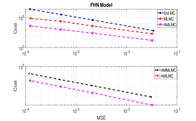
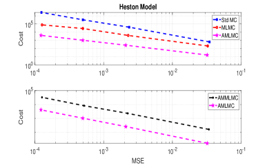
Figure 1: Cost versus MSE for the forward problem.

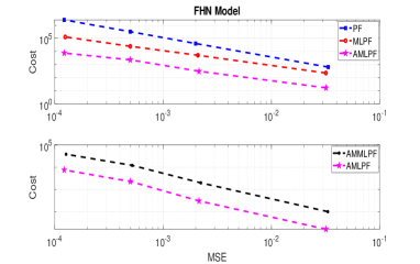
Figure 2: Cost versus MSE for the filtering problem.

Table 4: Estimated rates of cost against MSE. Left: Forward problem. Right: Filtering problem.

Model	Std MC	MLMC	AMLMC
FHN	-1.48	-1.1	-1.03
Heston	-1.47	-1.11	-1.05

Model	PF	MLPF	AMLPF
FHN	-1.46	-1.17	-1.11
Heston	-1.49	-1.24	-1.14

5 Conclusion

Our work has investigated the use of a non-degenerate weak second order scheme within the multilevel Monte Carlo (MLMC) framework, under the objective of an efficient estimation of expectations w.r.t the law of a wide class of diffusion processes, including hypo-elliptic diffusions. This latter is an important class of SDEs with numerous uses in applications. We first proved that our scheme has a strong error 1. Then, in the context of MLMC, we developed a new antithetic estimator based on our weak second order scheme which achieves the optimal cost rate $\mathcal{O}(\varepsilon^{-2})$, $\varepsilon>0$, to obtain a MSE of $\mathcal{O}(\varepsilon^{2})$. Such an optimal cost rate is also reported for the different antithetic MLMC approach of [10] which makes use of a truncated Milstein scheme of weak error 1. The new antithetic estimator is shown to possess two major benefits versus the one of [10]: (i) due to the higher order weak convergence, our estimator is expected to be more efficient for a finite maximum level of discretization $L$ used in practice; (ii) we have analytically showen that for small-noise diffusions the variance of the new antithetic estimator will be smaller than that of [10]. As an application, we have proposed an antithetic multilevel particle filter (AMLPF) by building upon previous works [17, 23] for the purposes of efficient filtering of diffusion processes from observations. Our simulation studies are in support of the anticipated cost of the proposed AMLPF being $\mathcal{O}(\varepsilon^{-2}\log(\varepsilon)^{2})$ to achieve an MSE of $\mathcal{O}(\varepsilon^{2})$. Also, all our numerics support the understanding that the new antithetic estimator using the weak second order scheme outperforms the antithetic Milstein scheme-based estimator in both forward/filtering problems.

We emphasize that our numerical scheme is locally non-degenerate under both elliptic/hypo-elliptic settings, whereas the truncated Milstein scheme is degenerate in the hypo-elliptic case. The non-degeneracy of the scheme makes possible its deployment within particle filters with guided proposals so that stochastic weights required to be assigned to particles are well-defined and available as the ratio of products involving the density expression for the numerical scheme and the proposal. The exploration of this direction is left for future work.

Acknowledgements

YI was supported by the Additional Funding Programme for Mathematical Sciences, delivered by EPSRC (EP/V521917/1) and the Heilbronn Institute for Mathematical Research. AJ was supported by SDS CUHK, Shenzhen.

Appendix A Proofs

A.1 Structure

This appendix contains the proofs of the results in the main text along with some technical results. It is meant to be read in order. The structure of this appendix is as follows. In Section A.2 we give the proof of Proposition 2.1. In Section A.3 we give the proof of Lemma 2.1. Then in Section A.4 several technical results are given, which are needed for the proof of Theorem 2.1, the latter of which can be found in Section A.5.

A.2 Proof of Proposition 2.1

Proof.

Let $1\leq i\leq 2^{\ell}$. We have

$$\mathcal{S}_{i}\equiv\mathbb{E}\Bigl{[}\max_{0\leq k\leq i}\|X_{t_{k}}-\bar{X}_{t_{k}}\|^{p}\Bigr{]}\leq N^{p-1}\sum_{1\leq j\leq N}\mathbb{E}\Bigl{[}\max_{0\leq k\leq i}|X_{t_{k}}^{j}-\bar{X}^{j}_{t_{k}}|^{p}\Bigr{]},$$ (34)

where we exploited the following inequality to obtain the above bound:

$$\Bigl{(}\sum_{1\leq j\leq N}|x_{j}|\Bigr{)}^{p}\leq N^{p-1}\sum_{1\leq j\leq N}|x_{j}|^{p},\quad x=(x_{1},\ldots,x_{N})\in\mathbb{R}^{N}.$$ (35)

We will show that for any $p\geq 2$, there exixts a constant $C>0$ such that

$$\mathcal{S}_{i}\leq C\Bigl{(}\Delta_{\ell}^{p/2}+\sum_{0\leq n\leq i-1}\mathcal{S}_{n}\cdot\Delta_{\ell}\Bigr{)},$$ (36)

which leads to the conclusion due to the discrete Gronwall’s inequality. We have for $0\leq k\leq i$,

$$X_{t_{k}}^{j}-\bar{X}^{j}_{t_{k}}=\sum_{0\leq n\leq k-1}\sum_{0\leq m\leq d}\int_{t_{n}}^{t_{n+1}}\bigl{(}\sigma_{m}^{j}(X_{s})-\sigma_{m}^{j}(\bar{X}_{t_{n}})\bigr{)}dB_{s}^{m}$$

$$\quad-\sum_{0\leq n\leq k-1}\sum_{0\leq m_{1},m_{2}\leq d}\mathscr{L}_{m_{1}}\sigma_{m_{2}}^{j}(\bar{X}_{t_{n}})\Delta\eta_{t_{n+1},t_{n}}^{m_{1}m_{2}}-\tfrac{1}{2}\sum_{0\leq n\leq k-1}\sum_{1\leq m_{1}<m_{2}\leq d}\bigl{[}\sigma_{m_{1}},\sigma_{m_{2}}\bigr{]}^{j}(\bar{X}_{t_{n}})\Delta\widetilde{A}_{t_{n+1},t_{n}}^{m_{1}m_{2}}.$$

Itô-Taylor expansion for $\sigma_{m}^{j}(X_{s}),\,s\in[t_{n},t_{n+1}]$ yields

$$X_{t_{k}}^{j}-\bar{X}^{j}_{t_{k}}=\sum_{0\leq n\leq k-1}\sum_{0\leq m\leq d}\bigl{(}\sigma_{m}^{j}(X_{t_{n}})-\sigma_{m}^{j}(\bar{X}_{t_{n}})\bigr{)}\Delta B^{m}_{t_{n+1},t_{n}}$$

$$\qquad+\tfrac{1}{2}\sum_{0\leq n\leq k-1}\sum_{1\leq m_{1},m_{2}\leq d}\bigl{(}\mathscr{L}_{m_{1}}\sigma_{m_{2}}^{j}(X_{t_{n}})-\mathscr{L}_{m_{1}}\sigma_{m_{2}}^{j}(\bar{X}_{t_{n}})\bigr{)}\bigl{\{}\Delta B_{t_{n+1},t_{n}}^{m_{1}}\Delta B_{t_{n+1},t_{n}}^{m_{2}}-\Delta_{\ell}\mathbf{1}_{m_{1}=m_{2}}\bigr{\}}$$

$$\qquad-\tfrac{1}{2}\sum_{0\leq n\leq k-1}\sum_{1\leq m_{1}<m_{2}\leq d}\Bigl{\{}[\sigma_{m_{1}},\sigma_{m_{2}}]^{j}(X_{t_{n}})\Delta A_{t_{n+1},t_{n}}^{m_{1}m_{2}}+[\sigma_{m_{1}},\sigma_{m_{2}}]^{j}(\bar{X}_{t_{n}})\Delta\widetilde{A}_{t_{n+1},t_{n}}^{m_{1}m_{2}}\Bigr{\}}$$

$$\qquad+\sum_{0\leq n\leq k-1}\bigl{(}\mathscr{M}_{t_{n+1},t_{n}}^{j}+\mathscr{N}_{t_{n+1},t_{n}}^{j}\bigr{)},$$ (37)

where the terms $\mathscr{M}_{t_{n+1},t_{n}}^{j}$, $\mathscr{N}_{t_{n+1},t_{n}}^{j}$ are specified as follows: $\mathbb{E}\bigl{[}\mathscr{M}_{t_{n+1},t_{n}}^{j}|\mathcal{F}_{t_{n}}\bigr{]}=0$ for $0\leq n\leq k-1$ and it holds under Assumption 2.1 that for any $p\geq 2$, there exist constants $C_{1},C_{2}>0$ such that

$$\max_{0\leq n\leq k-1}\mathbb{E}\bigl{[}|\mathscr{M}_{t_{n+1},t_{n}}^{j}|^{p}\bigr{]}\leq C_{1}\Delta_{\ell}^{3p/2},\qquad\max_{0\leq n\leq k-1}\mathbb{E}\bigl{[}|\mathscr{N}_{t_{n+1},t_{n}}^{j}|^{p}\bigr{]}\leq C_{2}\Delta_{\ell}^{2p}.$$ (38)

Thus, the inequality (35) yields

$$\mathbb{E}\Bigl{[}\max_{0\leq k\leq i}\bigl{|}X_{t_{k}}^{j}-\bar{X}_{t_{k}}^{j}\bigr{|}^{p}\Bigr{]}\leq C_{p}\sum_{1\leq\alpha\leq 6}\mathscr{T}_{i}^{(\alpha),j}$$ (39)

for some constant $C_{p}>0$, where we have set:

$$\mathscr{T}_{i}^{(1),j}=\mathbb{E}\Bigl{[}\max_{0\leq k\leq i}\bigl{|}\sum_{0\leq n\leq k-1}\bigl{(}\sigma_{0}^{j}(X_{t_{n}})-\sigma_{0}^{j}(\bar{X}_{t_{n}})\bigr{)}\Delta_{\ell}\bigr{|}^{p}\Bigr{]};$$

$$\mathscr{T}_{i}^{(2),j}=\mathbb{E}\Bigl{[}\max_{0\leq k\leq i}\bigl{|}\sum_{0\leq n\leq k-1}\sum_{1\leq m\leq d}\bigl{(}\sigma_{m}^{j}(X_{t_{n}})-\sigma_{m}^{j}(\bar{X}_{t_{n}})\bigr{)}\Delta B^{m}_{t_{n+1},t_{n}}\bigr{|}^{p}\Bigr{]};$$

$$\mathscr{T}_{i}^{(3),j}$$

$$=\mathbb{E}\Bigl{[}\max_{0\leq k\leq i}\bigl{|}\sum_{0\leq n\leq k-1}\sum_{1\leq m_{1},m_{2}\leq d}\bigl{(}\mathscr{L}_{m_{1}}\sigma_{m_{2}}^{j}(X_{t_{n}})-\mathscr{L}_{m_{1}}\sigma_{m_{2}}^{j}(\bar{X}_{t_{n}})\bigr{)}\bigl{\{}\Delta B_{t_{n+1},t_{n}}^{m_{1}}\Delta B_{t_{n+1},t_{n}}^{m_{2}}-\Delta_{\ell}\mathbf{1}_{m_{1}=m_{2}}\bigr{\}}\bigr{|}^{p}\Bigr{]};$$

$$\mathscr{T}_{i}^{(4),j}=\mathbb{E}\Bigl{[}\max_{0\leq k\leq i}\bigl{|}\sum_{0\leq n\leq k-1}\sum_{1\leq m_{1}<m_{2}\leq d}\bigl{\{}[\sigma_{m_{1}},\sigma_{m_{2}}]^{j}(X_{t_{n}})\Delta A_{t_{n+1},t_{n}}^{m_{1}m_{2}}+[\sigma_{m_{1}},\sigma_{m_{2}}]^{j}(\bar{X}_{t_{n}})\Delta\widetilde{A}_{t_{n+1},t_{n}}^{m_{1}m_{2}}\bigr{\}}\bigr{|}^{p}\Bigr{]};$$

$$\mathscr{T}_{i}^{(5),j}=\mathbb{E}\Bigl{[}\max_{0\leq k\leq i}\bigl{|}\sum_{0\leq n\leq k-1}\mathscr{M}_{t_{n+1},t_{n}}^{j}\bigr{|}^{p}\Bigr{]},\qquad\mathscr{T}_{i}^{(6),j}=\mathbb{E}\Bigl{[}\max_{0\leq k\leq i}\bigl{|}\sum_{0\leq n\leq k-1}\mathscr{N}_{t_{n+1},t_{n}}^{j}\bigr{|}^{p}\Bigr{]}.$$

Applying the inequality (35), we have under Assumption 2.1 that

$$\mathscr{T}^{(1),j}_{i} \leq i^{p-1}\sum_{0\leq n\leq i-1}\mathbb{E}\bigl{[}|\sigma_{0}^{j}(X_{t_{n}})-\sigma_{0}^{j}(\bar{X}_{t_{n}})|^{p}\bigr{]}\Delta_{\ell}^{p}\leq c_{1}(i\Delta_{\ell})^{p-1}\sum_{0\leq n\leq i-1}\mathcal{S}_{n}\cdot\Delta_{\ell}$$

$$\leq c_{1}T^{p-1}\sum_{0\leq n\leq i-1}\mathcal{S}_{n}\cdot\Delta_{\ell}$$

for some constant $c_{1}>0$ independent of $\Delta_{\ell}$ since $i\Delta_{\ell}\leq T$. Similarly we have

$$\mathscr{T}^{(6),j}_{i}\leq i^{p-1}\sum_{0\leq n\leq i-1}\mathbb{E}\bigl{[}|\mathscr{N}_{t_{n+1},t_{n}}^{j}|^{p}\bigr{]}\leq c_{6}T^{p}\Delta_{\ell}^{p}$$ (40)

for some constant $c_{6}>0$. We consider the other four terms. Since they involve martingales, we make use of the discrete Burkholder-Davis-Gundy inequality to obtain:

$$\mathscr{T}_{i}^{(2),j} \leq c_{2,1}\mathbb{E}\Bigl{[}\Bigl{(}\sum_{0\leq n\leq i-1}\sum_{1\leq m\leq d}\bigl{\{}(\sigma_{m}^{j}(X_{t_{n}})-\sigma_{m}^{j}(\bar{X}_{t_{n}}))\Delta B_{t_{n+1},t_{n}}^{m}\bigr{\}}^{2}\Bigr{)}^{p/2}\Bigr{]}$$

$$\leq i^{p/2-1}\sum_{0\leq n\leq i-1}\mathbb{E}\Bigl{[}\Bigl{|}\sum_{1\leq m\leq d}\bigl{\{}(\sigma_{m}^{j}(X_{t_{n}})-\sigma_{m}^{j}(\bar{X}_{t_{n}}))\Delta B_{t_{n+1},t_{n}}^{m}\bigr{\}}^{2}\Bigr{|}^{p/2}\Bigr{]}$$

$$\leq c_{2,2}\,i^{p/2-1}\sum_{0\leq n\leq i-1}\sum_{1\leq m\leq d}\mathbb{E}\Bigl{[}\Bigl{|}(\sigma_{m}^{j}(X_{t_{n}})-\sigma_{m}^{j}(\bar{X}_{t_{n}}))\Delta B_{t_{n+1},t_{n}}^{m}\Bigr{|}^{p}\Bigr{]}$$

$$\leq c_{2,3}\,i^{p/2-1}\sum_{0\leq n\leq i-1}\mathcal{S}_{n}\cdot\Delta_{\ell}^{p/2}\leq c_{2,3}\,T^{p/2-1}\sum_{0\leq n\leq i-1}\mathcal{S}_{n}\cdot\Delta_{\ell}$$

for some constants $c_{2,1},c_{2,2},c_{2,3}>0$, where we applied (35) in the second and third inequality. Similarly we have that

$$\mathscr{T}_{i}^{(3),j} \leq c_{3}i^{p/2-1}\sum_{0\leq n\leq i-1}\mathcal{S}_{n}\cdot\Delta_{\ell}^{p}\leq c_{3}T^{p/2-1}\Delta_{\ell}^{p/2}\sum_{0\leq n\leq i-1}\mathcal{S}_{n}\cdot\Delta_{\ell};$$

$$\mathscr{T}_{i}^{(5),j} \leq c_{5,1}\,i^{p/2-1}\sum_{0\leq n\leq i-1}\mathbb{E}\bigl{[}\bigl{|}\mathscr{M}_{t_{n+1},t_{n}}^{j}\bigr{|}^{p}\bigr{]}\leq c_{5,2}\,i^{p/2}\Delta_{\ell}^{3p/2}=c_{5,2}\,T^{p/2}\Delta_{\ell}^{p}$$

for some constants $c_{3},c_{5,1},c_{5,2}>0$. Finally, for the term $\mathscr{T}_{i}^{(4),j}$, we obtain

$$\mathscr{T}_{i}^{(4),j}\leq c_{4,1}i^{p/2-1}\sum_{0\leq n\leq i-1}\sum_{1\leq m_{1}<m_{2}\leq d}\mathbb{E}\bigl{[}|\Delta A_{t_{n+1},t_{n}}^{m_{1}m_{2}}|^{p}+|\Delta\widetilde{A}_{t_{n+1},t_{n}}^{m_{1}m_{2}}|^{p}\bigr{]}\leq c_{4,2}T^{p/2}\Delta_{\ell}^{p/2}$$ (41)

for some constants $c_{4,1},c_{4,2}>0$, where we used: $\mathbb{E}\bigl{[}|\Delta A_{t_{n+1},t_{n}}^{m_{1}m_{2}}|^{p}\bigr{]}=\mathcal{O}(\Delta_{\ell}^{p})$ and $\mathbb{E}\bigl{[}|\Delta\widetilde{A}_{t_{n+1},t_{n}}^{m_{1}m_{2}}|^{p}\bigr{]}=\mathcal{O}(\Delta_{\ell}^{p})$ for any $p\geq 2$. Note that $\sum_{0\leq n\leq i-1}\mathcal{S}_{n}$ does not appear in the upper bound of $\mathscr{T}_{i}^{(4),j}$. Thus, we obtain the inequality (36) and the proof is now complete. ∎

Remark A.1.

The error term $\mathscr{T}_{i}^{(4),j}$ appeared in the above proof is induced from the use of tractable random variables $\Delta\widetilde{A}_{t_{n+1},t_{n}}$ instead of intractable Lévy area $\Delta A_{t_{n+1},t_{n}}$ in the weak second order scheme (Weak-2). Due to the existence of the error term, the weak second order scheme attains the same rate of strong convergence as the E-M scheme or the truncated Milstein scheme (Truncated-Milstein).

A.3 Proof of Lemma 2.1

Proof.

Recall the definition of $\hat{X}^{f,[\ell]}$ and $\hat{X}^{c,[\ell-1]}$ in (13). The second order Taylor expansion yields:

$$\mathcal{P}_{f,\ell}^{\varphi} \equiv\tfrac{1}{2}(\varphi(\bar{X}_{T}^{f,[\ell]})+\varphi(\widetilde{X}_{T}^{f,[\ell]}))=\varphi(\hat{X}_{T}^{f,[\ell]})+\tfrac{1}{8}\bigl{(}\bar{X}_{T}^{f,[\ell]}-\widetilde{X}_{T}^{f,[\ell]}\bigr{)}^{\top}{\partial^{2}}\varphi(\xi_{1})\bigl{(}\bar{X}_{T}^{f,[\ell]}-\widetilde{X}_{T}^{f,[\ell]}\bigr{)};$$

$$\mathcal{P}_{c,\ell-1}^{\varphi} \equiv\tfrac{1}{2}(\varphi(\bar{X}_{T}^{c,[\ell-1]})+\varphi(\widetilde{X}_{T}^{c,[\ell-1]}))$$

$$=\varphi(\hat{X}_{T}^{c,[\ell-1]})+\tfrac{1}{8}\bigl{(}\bar{X}_{T}^{c,[\ell-1]}-\widetilde{X}_{T}^{c,[\ell-1]}\bigr{)}^{\top}{\partial^{2}}\varphi(\xi_{2})\bigl{(}\bar{X}_{T}^{c,[\ell-1]}-\widetilde{X}_{T}^{c,[\ell-1]}\bigr{)},$$

for some variables $\xi_{1},\xi_{2}\in\mathbb{R}^{N}$. Thus, we have:

$$\mathcal{P}_{f,\ell}^{\varphi}-\mathcal{P}_{c,\ell-1}^{\varphi} =\partial\varphi(\xi_{3})\bigl{(}\hat{X}_{T}^{f,[\ell]}-\hat{X}_{T}^{c,[\ell-1]}\bigr{)}+\tfrac{1}{8}\bigl{(}\bar{X}_{T}^{f,[\ell]}-\widetilde{X}_{T}^{f,[\ell]}\bigr{)}^{\top}{\partial^{2}}\varphi(\xi_{1})\bigl{(}\bar{X}_{T}^{f,[\ell]}-\widetilde{X}_{T}^{f,[\ell]}\bigr{)}$$

$$\qquad-\tfrac{1}{8}\bigl{(}\bar{X}_{T}^{c,[\ell-1]}-\widetilde{X}_{T}^{c,[\ell-1]}\bigr{)}^{\top}{\partial^{2}}\varphi(\xi_{2})\bigl{(}\bar{X}_{T}^{c,[\ell-1]}-\widetilde{X}_{T}^{c,[\ell-1]}\bigr{)},$$ (42)

for some $\xi_{3}\in\mathbb{R}^{N}$. The rest of the proof is the same as that of [10, Lemma 2.2]. ∎

A.4 Technical results for Theorem 2.1

Lemma A.1.

Let $1\leq j\leq N$, $1\leq\ell\leq L$, $0\leq k\leq 2^{\ell-1}-1$ and $t_{k}=k\Delta_{\ell-1}$. It holds that

$$\bar{X}^{f,[\ell],j}_{t_{k+1}} =\bar{X}^{f,[\ell],j}_{t_{k}}+\sum_{0\leq m\leq d}\sigma_{m}^{j}\bigl{(}\bar{X}^{f,[\ell]}_{t_{k}}\bigr{)}\Delta B_{t_{k+1},t_{k}}^{m}+\sum_{0\leq m_{1},m_{2}\leq d}\mathscr{L}_{m_{1}}\sigma_{m_{2}}^{j}\bigl{(}\bar{X}^{f,[\ell]}_{t_{k}}\bigr{)}\Delta\eta_{t_{k+1},t_{k}}^{m_{1}m_{2}}$$

$$\qquad-\tfrac{1}{2}\sum_{1\leq m_{1},m_{2}\leq d}\mathscr{L}_{m_{1}}\sigma_{m_{2}}^{j}\bigl{(}\bar{X}^{f,[\ell]}_{t_{k}}\bigr{)}\bigl{(}\Delta B_{t_{k+1},t_{k+1/2}}^{m_{1}}\Delta B_{t_{k+1/2},t_{k}}^{m_{2}}-\Delta B_{t_{k+1/2},t_{k}}^{m_{1}}\Delta B_{t_{k+1},t_{k+1/2}}^{m_{2}}\bigr{)}$$

$$\qquad+\tfrac{1}{2}\sum_{1\leq m_{1}<m_{2}\leq d}\bigl{[}\sigma_{m_{1}},\sigma_{m_{2}}\bigr{]}^{j}\bigl{(}\bar{X}^{f,[\ell]}_{t_{k}}\bigr{)}\bigl{(}\Delta B^{m_{1}}_{t_{k+1/2},t_{k}}\Delta\widetilde{B}^{m_{2}}_{t_{k+1/2},t_{k}}+\Delta B^{m_{1}}_{t_{k+1},t_{k+1/2}}\Delta\widetilde{B}^{m_{2}}_{t_{k+1},t_{k+1/2}}\bigr{)}$$

$$\qquad+\bar{\mathscr{M}}^{f,j}_{t_{k+1},t_{k}}+\bar{\mathscr{N}}^{f,j}_{t_{k+1},t_{k}},$$ (43)

where the remainder terms are specified as follows:

$$\mathbb{E}\bigl{[}\bar{\mathscr{M}}^{f,j}_{t_{k+1},t_{k}}|\mathcal{F}_{t_{k}}\bigr{]}=0,\quad 0\leq k\leq 2^{\ell-1}-1,$$ (44)

and for any $p\geq 2$ there exist constants $C_{1},C_{2}>0$ such that

$$\max_{0\leq k\leq 2^{\ell-1}-1}\mathbb{E}\bigl{[}|\bar{\mathscr{M}}^{f,j}_{t_{k+1},t_{k}}|^{p}\bigr{]}\leq C_{1}\Delta_{\ell-1}^{3p/2},\qquad\max_{0\leq k\leq 2^{\ell-1}-1}\mathbb{E}\bigl{[}|\bar{\mathscr{N}}^{f,j}_{t_{k+1},t_{k}}|^{p}\bigr{]}\leq C_{2}\Delta_{\ell-1}^{2p}.$$ (45)

Similarly, it holds that

$$\widetilde{X}^{f,[\ell],j}_{t_{k+1}} =\widetilde{X}^{f,[\ell],j}_{t_{k}}+\sum_{0\leq m\leq d}\sigma_{m}^{j}\bigl{(}\widetilde{X}^{f,[\ell]}_{t_{k}}\bigr{)}\Delta B_{t_{k+1},t_{k}}^{m}+\sum_{0\leq m_{1},m_{2}\leq d}\mathscr{L}_{m_{1}}\sigma_{m_{2}}^{j}\bigl{(}\widetilde{X}^{f,[\ell]}_{t_{k}}\bigr{)}\Delta\eta_{t_{k+1},t_{k}}^{m_{1}m_{2}}$$

$$\qquad+\tfrac{1}{2}\sum_{1\leq m_{1},m_{2}\leq d}\mathscr{L}_{m_{1}}\sigma_{m_{2}}^{j}\bigl{(}\widetilde{X}^{f,[\ell]}_{t_{k}}\bigr{)}\bigl{(}\Delta B_{t_{k+1},t_{k+1/2}}^{m_{1}}\Delta B_{t_{k+1/2},t_{k}}^{m_{2}}-\Delta B_{t_{k+1/2},t_{k}}^{m_{1}}\Delta B_{t_{k+1},t_{k+1/2}}^{m_{2}}\bigr{)}$$

$$\qquad-\tfrac{1}{2}\sum_{1\leq m_{1}<m_{2}\leq d}\bigl{[}\sigma_{m_{1}},\sigma_{m_{2}}\bigr{]}^{j}\bigl{(}\widetilde{X}^{f,[\ell]}_{t_{k}}\bigr{)}\bigl{(}\Delta B^{m_{1}}_{t_{k+1/2},t_{k}}\Delta\widetilde{B}^{m_{2}}_{t_{k+1/2},t_{k}}+\Delta B^{m_{1}}_{t_{k+1},t_{k+1/2}}\Delta\widetilde{B}^{m_{2}}_{t_{k+1},t_{k+1/2}}\bigr{)}$$

$$\qquad+\widetilde{\mathscr{M}}_{t_{k+1},t_{k}}^{\,f,j}+\widetilde{\mathscr{N}}_{t_{k+1},t_{k}}^{\,f,j},$$ (46)

where the remainder terms $\widetilde{\mathscr{M}}_{t_{k+1},t_{k}}^{\,f,j}$ and $\widetilde{\mathscr{N}}_{t_{k+1},t_{k}}^{\,f,j}$ satisfy the same property as $\bar{\mathscr{M}}_{t_{k+1},t_{k}}^{f,j}$ and $\bar{\mathscr{N}}_{t_{k+1},t_{k}}^{f,j}$, respectively.

Proof.

From the definition of the fine discretization scheme (8), we have:

$$\bar{X}_{t_{k+1}}^{{f},[\ell],j} =\bar{X}_{t_{k}}^{{f},[\ell],j}+\sum_{0\leq m\leq d}\Bigl{\{}\sigma_{m}^{j}(\bar{X}_{t_{k}}^{f,[\ell]})\Delta B_{t_{k+1/2},t_{k}}^{m}+\sigma_{m}^{j}(\bar{X}_{t_{k+1/2}}^{f,[\ell]})\Delta B_{t_{k+1},t_{k+1/2}}^{m}\Bigr{\}}$$

$$\qquad+\sum_{0\leq m_{1},m_{2}\leq d}\Bigl{\{}\mathscr{L}_{m_{1}}\sigma_{m_{2}}^{j}\bigl{(}\bar{X}_{t_{k}}^{f,[\ell]}\bigr{)}\Delta\eta_{t_{k+1/2},t_{k}}^{m_{1}m_{2}}+\mathscr{L}_{m_{1}}\sigma_{m_{2}}^{j}\bigl{(}\bar{X}_{t_{k+1/2}}^{f,[\ell]}\bigr{)}\Delta\eta_{t_{k+1},t_{k+1/2}}^{m_{1}m_{2}}\Bigr{\}}$$

$$\qquad+\tfrac{1}{2}\sum_{1\leq m_{1}<m_{2}\leq d}\Bigl{\{}[\sigma_{m_{1}},\sigma_{m_{2}}]^{j}\bigl{(}\bar{X}_{t_{k}}^{f,[\ell]}\bigr{)}\Delta B^{m_{1}}_{t_{k+1/2},t_{k}}\Delta\widetilde{B}^{m_{2}}_{t_{k+1/2},t_{k}}$$

$$\qquad\qquad\qquad\qquad\qquad+[\sigma_{m_{1}},\sigma_{m_{2}}]^{j}\bigl{(}\bar{X}_{t_{k+1/2}}^{f,[\ell]}\bigr{)}\Delta B^{m_{1}}_{t_{k+1},t_{k+1/2}}\Delta\widetilde{B}^{m_{2}}_{t_{k+1},t_{k+1/2}}\Bigr{\}}.$$ (47)

Itô-Taylor expansion gives

$$\sigma_{m}^{j}(\bar{X}_{t_{k+1/2}}^{f,[\ell]})=\sigma_{m}^{j}(\bar{X}_{t_{k}}^{f,[\ell]})+\sum_{0\leq m_{1}\leq d}\mathscr{L}_{m_{1}}\sigma^{j}_{m}(\bar{X}_{t_{k}}^{f,[\ell]})\Delta B_{t_{k+1/2},t_{k}}^{m_{1}}+\mathscr{E}_{t_{k+1/2},t_{k}}^{f,j},\quad 0\leq m\leq d,$$ (48)

where under Assumption 2.1 the remainder term $\mathscr{E}_{t_{k+1/2},t_{k}}^{f,j}$ is specified as follows: for any $p\geq 2$, there exists a constant $C>0$ such that

$$\max_{0\leq k\leq 2^{\ell-1}-1}\mathbb{E}\bigl{[}|\mathscr{E}_{t_{k+1/2},t_{k}}^{f,j}|^{p}\bigr{]}\leq C\Delta_{\ell}^{p}.$$ (49)

Furthermore, Taylor expansion gives:

$$\mathscr{L}_{m_{1}}\sigma_{m_{2}}^{j}(\bar{X}_{t_{k+1/2}}^{f,[\ell]}) =\mathscr{L}_{k_{1}}\sigma_{k_{2}}^{j}(\bar{X}_{t_{k}}^{f,[\ell]})+\sum_{1\leq i\leq N}\partial_{i}\bigl{(}\mathscr{L}_{m_{1}}\sigma_{m_{2}}^{j}\bigr{)}(\xi_{1})\bigl{(}\bar{X}_{t_{k+1/2}}^{f,[\ell],i}-\bar{X}_{t_{k}}^{f,[\ell],i}\bigr{)};$$ (50)

$$[\sigma_{m_{1}},\sigma_{m_{2}}]^{j}(\bar{X}_{t_{k+1/2}}^{f,[\ell]}) =[\sigma_{m_{1}},\sigma_{m_{2}}]^{j}(\bar{X}_{t_{k}}^{f,[\ell]})+\sum_{1\leq i\leq N}\partial_{i}\bigl{(}[\sigma_{k_{1}},\sigma_{k_{2}}]^{j}\bigr{)}(\xi_{2})(\bar{X}_{t_{k+1/2}}^{f,[\ell],i}-\bar{X}_{t_{k}}^{f,[\ell],i}),$$ (51)

for some variables $\xi_{1},\xi_{2}\in\mathbb{R}^{N}$. Notice that under Assumption 2.1 it holds that for any $p\geq 2$ and $1\leq j\leq N$, there exists a constant $C>0$ such that

$$\max_{0\leq k\leq 2^{\ell-1}-1}\mathbb{E}\bigl{[}|\bar{X}_{t_{k+1/2}}^{f,[\ell],j}-\bar{X}_{t_{k}}^{f,[\ell],j}|^{p}\bigr{]}\leq C\Delta_{\ell-1}^{p/2}.$$

Since we have that

$$\Delta B^{m_{1}}_{t_{k+1},t_{k}}\Delta B^{m_{2}}_{t_{k+1},t_{k}} =\Delta B^{m_{1}}_{t_{k+1},t_{k+1/2}}\Delta B^{m_{2}}_{t_{k+1},t_{k+1/2}}+\Delta B^{m_{1}}_{t_{k+1},t_{k+1/2}}\Delta B^{m_{2}}_{t_{k+1/2},t_{k}}$$

$$\quad+\Delta B^{m_{1}}_{t_{k+1/2},t_{k}}\Delta B^{m_{2}}_{t_{k+1},t_{k+1/2}}+\Delta B^{m_{1}}_{t_{k+1/2},t_{k}}\Delta B^{m_{2}}_{t_{k+1/2},t_{k}},$$ (52)

substituting (48), (50) and (51) into (A.4) together with (A.4), we obtain

$$\bar{X}_{t_{k+1}}^{{f},[\ell],j}=\bar{X}_{t_{k}}^{{f},[\ell],j}+\sum_{0\leq m\leq d}\sigma_{m}^{j}(\bar{X}_{t_{k}}^{f,[\ell]})\Delta B_{t_{k+1},t_{k}}^{m}+\sum_{0\leq m_{1},m_{2}\leq d}\mathscr{L}_{m_{1}}\sigma_{m_{2}}^{j}\bigl{(}\bar{X}_{t_{k}}^{f,[\ell]}\bigr{)}\Delta\eta_{t_{k+1},t_{k}}^{m_{1}m_{2}}$$

$$\quad-\tfrac{1}{2}\sum_{1\leq m_{1},m_{2}\leq d}\mathscr{L}_{m_{1}}\sigma_{m_{2}}^{j}\bigl{(}\bar{X}^{f,[\ell]}_{t_{k}}\bigr{)}\bigl{(}\Delta B_{t_{k+1},t_{k+1/2}}^{m_{1}}\Delta B_{t_{k+1/2},t_{k}}^{m_{2}}-\Delta B_{t_{k+1/2,k}}^{m_{1}}\Delta B_{t_{k+1},t_{k+1/2}}^{m_{2}}\bigr{)}$$

$$\quad+\tfrac{1}{2}\sum_{1\leq m_{1}<m_{2}\leq d}[\sigma_{m_{1}},\sigma_{m_{2}}]^{j}\bigl{(}\bar{X}_{t_{k}}^{f,[\ell]}\bigr{)}\bigl{(}\Delta B^{m_{1}}_{t_{k+1},t_{k+1/2}}\Delta\widetilde{B}^{m_{2}}_{t_{k+1},t_{k+1/2}}+\Delta B^{m_{1}}_{t_{k+1/2},t_{k}}\Delta\widetilde{B}^{m_{2}}_{t_{k+1/2},t_{k}}\bigr{)}$$

$$\quad+\bar{\mathscr{M}}_{t_{k+1},t_{k}}^{f,j}+\bar{\mathscr{N}}_{t_{k+1},t_{k}}^{f,j},$$ (53)

where the remainder terms $\bar{\mathscr{M}}_{t_{k+1},t_{k}}^{f,j}$ and $\bar{\mathscr{N}}_{t_{k+1},t_{k}}^{f,j}$ have the properties stated in Lemma A.1. The assertion for $\widetilde{X}^{f,[\ell]}$ follows from the same discussion above, and the proof is now complete. ∎

Lemma A.2.

Let $1\leq j\leq N$, $1\leq\ell\leq L$, $0\leq k\leq 2^{\ell-1}-1$ and $t_{k}=k\Delta_{\ell-1}$. It holds that

$$\begin{aligned} \hat{X}^{f,[\ell],j}_{t_{k+1}}&=\hat{X}^{f,[\ell],j}_{t_{k}}+\sum_{0\leq m\leq d}\sigma_{m}^{j}(\hat{X}^{f,[\ell]}_{t_{k}})\Delta B_{t_{k+1},t_{k}}^{m}+\sum_{1\leq m_{1},m_{2}\leq d}\mathscr{L}_{m_{1}}\sigma_{m_{2}}^{j}(\hat{X}_{t_{k}}^{f,[\ell]})\Delta\eta_{t_{k+1},t_{k}}^{m_{1}m_{2}}\\ &\quad+\hat{\mathscr{M}}_{t_{k+1},t_{k}}^{f,j}+\hat{\mathscr{N}}_{t_{k+1},t_{k}}^{f,j},\end{aligned}$$ (54)

where the remainder terms are specified as follows:

$$\mathbb{E}\bigl{[}\hat{\mathscr{M}}_{t_{k+1},t_{k}}^{f,j}|\mathcal{F}_{t_{k}}\bigr{]}=0,\quad 0\leq k\leq 2^{\ell-1}-1,$$ (55)

and for any $p\geq 2$, there exist constants $C_{1},C_{2}>0$ such that

$$\max_{0\leq k\leq 2^{\ell-1}-1}\mathbb{E}\bigl{[}|\hat{\mathscr{M}}_{t_{k+1},t_{k}}^{f,j}|^{p}\bigr{]}\leq C_{1}\Delta_{\ell-1}^{3p/2},\quad\max_{0\leq k\leq 2^{\ell-1}-1}\mathbb{E}\bigl{[}|\hat{\mathscr{N}}_{t_{k+1},t_{k}}^{f,j}|^{p}\bigr{]}\leq C_{2}\Delta_{\ell-1}^{2p}.$$ (56)

Proof.

Due to Lemma A.1, we get

$$\hat{X}_{t_{k+1}}^{f,[\ell],j} =\hat{X}_{t_{k}}^{f,[\ell],j}+\sum_{0\leq m\leq d}\sigma_{m}^{j}(\hat{X}_{t_{k}}^{f,[\ell]})\Delta B_{t_{k+1},t_{k}}^{m}+\sum_{1\leq m_{1},m_{2}\leq d}\mathscr{L}_{m_{1}}\sigma_{m_{2}}^{j}(\hat{X}_{t_{k}}^{f,[\ell]})\Delta\eta_{t_{k+1},t_{k}}^{m_{1}m_{2}}$$

$$\qquad+\sum_{1\leq i\leq 6}{\mathscr{E}}_{t_{k+1},t_{k}}^{(i),j}+\tfrac{1}{2}\bigl{\{}\bar{\mathscr{M}}_{t_{k+1},t_{k}}^{f,j}+\widetilde{\mathscr{M}}_{t_{k+1},t_{k}}^{\,f,j}+\bar{\mathscr{N}}_{t_{k+1},t_{k}}^{f,j}+\widetilde{\mathscr{N}}_{t_{k+1},t_{k}}^{\,f,j}\bigr{\}},$$ (57)

where we have set:

$${\mathscr{E}}_{t_{k+1},t_{k}}^{(1),j} =\sum_{1\leq m\leq d}\Bigl{(}\tfrac{1}{2}\sigma_{m}^{j}(\bar{X}^{f,[\ell]}_{t_{k}})+\tfrac{1}{2}\sigma_{m}^{j}(\widetilde{X}^{f,[\ell]}_{t_{k}})-\sigma_{m}^{j}(\hat{X}_{t_{k}}^{f,[\ell]})\Bigr{)}\Delta B_{t_{k+1},t_{k}}^{m};$$

$${\mathscr{E}}_{t_{k+1},t_{k}}^{(2),j} =\Bigl{(}\tfrac{1}{2}\sigma_{0}^{j}(\bar{X}_{t_{k}}^{f,[\ell]})+\tfrac{1}{2}\sigma_{0}^{j}(\widetilde{X}_{t_{k}}^{f,[\ell]})-\sigma_{0}^{j}(\hat{X}_{t_{k}}^{f,[\ell]})\Bigr{)}\Delta_{\ell-1}+\Bigl{(}\mathscr{L}_{0}\sigma_{0}^{j}(\bar{X}_{t_{k}}^{f,[\ell]})+\mathscr{L}_{0}\sigma_{0}^{j}(\widetilde{X}_{t_{k}}^{f,[\ell]})\Bigr{)}\tfrac{\Delta_{\ell-1}^{2}}{4};$$

$${\mathscr{E}}_{t_{k+1},t_{k}}^{(3),j} =\sum_{1\leq m_{1},m_{2}\leq d}\Bigl{(}\tfrac{1}{2}\mathscr{L}_{m_{1}}\sigma_{m_{2}}^{j}(\bar{X}_{t_{k}}^{f,[\ell]})+\tfrac{1}{2}\mathscr{L}_{m_{1}}\sigma_{m_{2}}^{j}(\widetilde{X}_{t_{k}}^{f,[\ell]})-\mathscr{L}_{m_{1}}\sigma_{m_{2}}^{j}(\hat{X}_{t_{k}}^{f,[\ell]})\Bigr{)}\Delta\eta_{t_{k+1},t_{k}}^{m_{1}m_{2}};$$

$${\mathscr{E}}_{t_{k+1},t_{k}}^{(4),j} =\tfrac{1}{2}\sum_{1\leq m\leq d}\Bigl{\{}\bigl{(}\mathscr{L}_{m}\sigma_{0}^{j}(\bar{X}_{t_{k}}^{f,[\ell]})+\mathscr{L}_{m}\sigma_{0}^{j}(\widetilde{X}_{t_{k}}^{f,[\ell]})\bigr{)}\Delta\eta_{t_{k+1},t_{k}}^{m0}$$

$$\qquad\qquad\qquad\qquad+\bigl{(}\mathscr{L}_{0}\sigma_{m}^{j}(\bar{X}_{t_{k}}^{f,[\ell]})+\mathscr{L}_{0}\sigma_{m}^{j}(\widetilde{X}_{t_{k}}^{f,[\ell]})\bigr{)}\Delta\eta_{t_{k+1},t_{k}}^{0m}\Bigr{\}};$$

$${\mathscr{E}}_{t_{k+1},t_{k}}^{(5),j} =-\tfrac{1}{4}\sum_{1\leq m_{1},m_{2}\leq d}\Bigl{\{}\bigl{(}\mathscr{L}_{m_{1}}\sigma_{m_{2}}^{j}(\bar{X}_{t_{k}}^{f,[\ell]})-\mathscr{L}_{m_{1}}\sigma_{m_{2}}^{j}(\widetilde{X}_{t_{k}}^{f,[\ell]})\bigr{)}$$

$$\qquad\qquad\qquad\qquad\times\bigl{(}\Delta B_{t_{k+1},t_{k+1/2}}^{m_{1}}\Delta B_{t_{k+1/2},t_{k}}^{m_{2}}-\Delta B_{t_{k+1/2},t_{k}}^{m_{1}}\Delta B_{t_{k+1},t_{k+1/2}}^{m_{2}}\bigr{)}\Bigr{\}};$$

$${\mathscr{E}}_{t_{k+1},t_{k}}^{(6),j} =\tfrac{1}{4}\sum_{1\leq m_{1}<m_{2}\leq d}\Bigl{\{}\bigl{(}[\sigma_{m_{1}},\sigma_{m_{2}}]^{j}(\bar{X}_{t_{k}}^{f,[\ell]})-[\sigma_{m_{1}},\sigma_{m_{2}}]^{j}(\widetilde{X}_{t_{k}}^{f,[\ell]})\bigr{)}$$

$$\qquad\qquad\qquad\qquad\times\bigl{(}\Delta B^{m_{1}}_{t_{k+1},t_{k+1/2}}\Delta\widetilde{B}^{m_{2}}_{t_{k+1},t_{k+1/2}}+\Delta B^{m_{1}}_{t_{k+1/2},t_{k}}\Delta\widetilde{B}^{m_{2}}_{t_{k+1/2},t_{k}}\bigr{)}\Bigr{\}}.$$

We immediately have that: for any $1\leq j\leq N$ and $0\leq k\leq 2^{\ell-1}-1$,

$$\mathbb{E}\bigl{[}{\mathscr{E}}_{t_{k+1},t_{k}}^{(i),j}|\mathcal{F}_{t_{k}}\bigr{]}=0,\qquad i\in\{1,3,4,5,6\}.$$ (58)

Second order Taylor expansion around $\hat{X}_{t_{k}}^{f,[\ell]}$ yields: for $g\in C_{b}^{2}(\mathbb{R}^{N};\mathbb{R})$,

$$\tfrac{1}{2}\bigl{(}g(\bar{X}_{t_{k}}^{f,[\ell]})+g(\widetilde{X}_{t_{k}}^{f,[\ell]})\bigr{)}-g(\hat{X}_{t_{k}}^{f,[\ell]})$$

$$\qquad=\tfrac{1}{16}\sum_{1\leq j_{1},j_{2}\leq N}\bigl{\{}\partial_{j_{1}}\partial_{j_{2}}g(\xi_{1})+\partial_{j_{1}}\partial_{j_{2}}g(\xi_{2})\bigr{\}}\cdot\bigl{(}\bar{X}_{t_{k}}^{f,[\ell],j_{1}}-\widetilde{X}_{t_{k}}^{f,[\ell],j_{1}}\bigr{)}\bigl{(}\bar{X}_{t_{k}}^{f,[\ell],j_{2}}-\widetilde{X}_{t_{k}}^{f,[\ell],j_{2}}\bigr{)};$$

$$g(\bar{X}_{t_{k}}^{f,[\ell]})-g(\widetilde{X}_{t_{k}}^{f,[\ell]})=\sum_{1\leq j\leq N}\partial_{j}g(\xi_{3})\cdot\bigl{(}\bar{X}_{t_{k}}^{f,[\ell],j}-\widetilde{X}_{t_{k}}^{f,[\ell],j}\bigr{)},$$

for some variables $\xi_{1},\xi_{2},\xi_{3}\in\mathbb{R}^{N}$. Thus, it follows under Assumption 2.1 that for any $p\geq 2$ there exist constants $C_{1},C_{2}>0$ such that for all $0\leq k\leq 2^{\ell-1}-1$,

$$\mathbb{E}\bigl{[}\bigl{|}\tfrac{1}{2}\bigl{(}g(\bar{X}_{t_{k}}^{f,[\ell]})+g(\widetilde{X}_{t_{k}}^{f,[\ell]})\bigr{)}-g(\hat{X}_{t_{k}}^{f,[\ell]})\bigr{|}^{p}\bigr{]}\leq C_{1}\Delta_{\ell-1}^{p};$$ (59)

$$\mathbb{E}\bigl{[}\bigl{|}g(\bar{X}_{t_{k}}^{f,[\ell]})-g(\widetilde{X}_{t_{k}}^{f,[\ell]})\bigr{|}^{p}\bigr{]}\leq C_{2}\Delta_{\ell-1}^{p/2},$$ (60)

where we made use of the following result that can be shown from Proposition 2.1 and the same argument for the proof of [10, Lemma 4.6]: for any $p\geq 2$,

$$\max_{0\leq k\leq 2^{\ell-1}-1}\mathbb{E}\bigl{[}|\bar{X}_{t_{k}}^{f,[\ell]}-\widetilde{X}_{t_{k}}^{f,[\ell]}|^{p}\bigr{]}\leq C\Delta_{\ell-1}^{p/2}$$ (61)

for some constant $C>0$. Then, we have that

$$\max_{0\leq k\leq 2^{\ell-1}-1}\mathbb{E}\bigl{[}|\mathscr{E}_{t_{k+1},t_{k}}^{(2),j}|^{p}\bigr{]}\leq C_{1}\Delta_{\ell-1}^{2p},\quad\max_{0\leq k\leq 2^{\ell-1}-1}\mathbb{E}\bigl{[}|{\mathscr{E}}_{t_{k+1},t_{k}}^{(i),j}|^{p}\bigr{]}=C_{2}\Delta_{\ell-1}^{3p/2},\quad i\in\{1,3,4,5,6\}$$ (62)

for some constants $C_{1},C_{2}>0$. Finally, we set

$$\hat{\mathscr{M}}_{t_{k+1},t_{k}}^{f,j}=\sum_{i\in\{1,3,4,5,6\}}\mathscr{E}_{t_{k+1},t_{k}}^{(i),j}+\tfrac{1}{2}\bigl{(}\bar{\mathscr{M}}_{t_{k+1},t_{k}}^{f,j}+\widetilde{\mathscr{M}}_{t_{k+1},t_{k}}^{\,f,j}\bigr{)},\quad\hat{\mathscr{N}}_{t_{k+1},t_{k}}^{f,j}=\mathscr{E}_{t_{k+1},t_{k}}^{(2),j}+\tfrac{1}{2}\bigl{(}\bar{\mathscr{N}}_{t_{k+1},t_{k}}^{f,j}+\widetilde{\mathscr{N}}_{t_{k+1},t_{k}}^{\,f,j}\bigr{)},$$

and the proof is complete. ∎

Lemma A.3.

Let $1\leq j\leq N$, $1\leq\ell\leq L$, $0\leq k\leq 2^{\ell-1}-1$ and $t_{k}=k\Delta_{\ell-1}$. It holds that

$$\begin{aligned} \hat{X}_{t_{k+1}}^{c,[\ell-1],j}&=\hat{X}_{t_{k}}^{c,[\ell-1],j}+\sum_{0\leq m\leq d}\sigma_{m}^{j}(\hat{X}_{t_{k}}^{c,[\ell-1]})\Delta B_{t_{k+1},t_{k}}^{m}+\sum_{1\leq m_{1},m_{2}\leq d}\mathscr{L}_{m_{1}}\sigma_{m_{2}}^{j}(\hat{X}_{t_{k}}^{c,[\ell-1]})\Delta\eta^{m_{1}m_{2}}_{t_{k+1},t_{k}}\\ &\quad+\hat{\mathscr{M}}_{t_{k+1},t_{k}}^{c,j}+\hat{\mathscr{N}}_{t_{k+1},t_{k}}^{c,j},\end{aligned}$$

where the remainder terms are specified as follows:

$$\mathbb{E}\bigl{[}\hat{\mathscr{M}}_{t_{k+1},t_{k}}^{c,j}|\mathcal{F}_{t_{k}}\bigr{]}=0,\quad 0\leq k\leq 2^{\ell-1}-1,$$ (63)

and for any $p\geq 2$ there exists a constant $C>0$ such that

$$\max_{0\leq k\leq 2^{\ell-1}-1}\mathbb{E}\bigl{[}|\hat{\mathscr{M}}_{t_{k+1},t_{k}}^{c,j}|^{p}\bigr{]}\leq C\Delta_{\ell-1}^{3p/2},\quad\max_{0\leq k\leq 2^{\ell-1}-1}\mathbb{E}\bigl{[}|\hat{\mathscr{N}}_{t_{k+1},t_{k}}^{c,j}|^{p}\bigr{]}\leq C\Delta_{\ell-1}^{2p}.$$ (64)

Proof.

From the discretizations (6) and (7), we have

$$\hat{X}_{t_{k+1}}^{c,[\ell-1],j} =\hat{X}_{t_{k}}^{c,[\ell-1],j}+\sum_{0\leq m\leq d}\sigma_{m}^{j}(\hat{X}_{t_{k}}^{c,[\ell-1]})\Delta B_{t_{k+1},t_{k}}^{m}+\sum_{1\leq m_{1},m_{2}\leq d}\mathscr{L}_{m_{1}}\sigma_{m_{2}}^{j}(\hat{X}_{t_{k}}^{c,[\ell-1]})\Delta\eta^{m_{1}m_{2}}_{t_{k+1},t_{k}}$$

$$\quad+\sum_{1\leq i\leq 5}\mathscr{R}_{t_{k+1},t_{k}}^{(i),j},$$

where we have defined

$$\mathscr{R}_{t_{k+1},t_{k}}^{(1),j} =\bigl{(}\tfrac{1}{2}\sigma_{0}^{j}(\bar{X}_{t_{k}}^{c,[\ell-1]})+\tfrac{1}{2}\sigma_{0}^{j}(\widetilde{X}_{t_{k}}^{c,[\ell-1]})-\sigma_{0}^{j}(\hat{X}_{t_{k}}^{c,[\ell-1]})\bigr{)}\Delta_{\ell-1}$$

$$\qquad+\bigl{(}\mathscr{L}_{0}\sigma_{0}^{j}(\bar{X}_{t_{k}}^{c,[\ell-1]})+\mathscr{L}_{0}\sigma_{0}^{j}(\widetilde{X}_{t_{k}}^{c,[\ell-1]})\bigr{)}\tfrac{\Delta_{\ell-1}^{2}}{4};$$

$$\mathscr{R}_{t_{k+1},t_{k}}^{(2),j} =\sum_{1\leq m\leq d}\bigl{(}\tfrac{1}{2}\sigma_{m}^{j}(\bar{X}_{t_{k}}^{c,[\ell-1]})+\tfrac{1}{2}\sigma_{m}^{j}(\widetilde{X}_{t_{k}}^{c,[\ell-1]})-\sigma_{m}^{j}(\hat{X}_{t_{k}}^{c,[\ell-1]})\bigr{)}\Delta B_{t_{k+1},t_{k}}^{m};$$

$$\mathscr{R}_{t_{k+1},t_{k}}^{(3),j} =\sum_{1\leq m_{1},m_{2}\leq d}\bigl{(}\tfrac{1}{2}\mathscr{L}_{m_{1}}\sigma_{m_{2}}^{j}(\bar{X}_{t_{k}}^{c,[\ell-1]})+\tfrac{1}{2}\mathscr{L}_{m_{1}}\sigma_{m_{2}}^{j}(\widetilde{X}_{t_{k}}^{c,[\ell-1]})-\mathscr{L}_{m_{1}}\sigma_{m_{2}}^{j}(\hat{X}_{t_{k}}^{c,[\ell-1]})\bigr{)}\Delta\eta_{t_{k+1},t_{k}}^{m_{1}m_{2}};$$

$$\mathscr{R}_{t_{k+1},t_{k}}^{(4),j} =\tfrac{1}{4}\sum_{1\leq m_{1}<m_{2}\leq d}\bigl{(}[\sigma_{m_{1}},\sigma_{m_{2}}]^{j}(\bar{X}_{t_{k}}^{c,[\ell-1]})-[\sigma_{m_{1}},\sigma_{m_{2}}]^{j}(\widetilde{X}_{t_{k}}^{c,[\ell-1]})\bigr{)}\Delta B_{t_{k+1},t_{k}}^{m_{1}}\Delta\widetilde{B}_{t_{k+1},t_{k}}^{m_{2}};$$

$$\mathscr{R}_{t_{k+1},t_{k}}^{(5),j} =\tfrac{1}{2}\sum_{1\leq m\leq d}\bigl{(}\mathscr{L}_{m}\sigma_{0}^{j}(\bar{X}_{t_{k}}^{c,[\ell-1]})+\mathscr{L}_{m}\sigma_{0}^{j}(\widetilde{X}_{t_{k}}^{c,[\ell-1]})\bigr{)}\Delta\eta_{t_{k+1},t_{k}}^{m0}$$

$$\quad+\tfrac{1}{2}\sum_{1\leq m\leq d}\bigl{(}\mathscr{L}_{0}\sigma_{m}^{j}(\bar{X}_{t_{k}}^{c,[\ell-1]})+\mathscr{L}_{0}\sigma_{m}^{j}(\widetilde{X}_{t_{k}}^{c,[\ell-1]})\bigr{)}\Delta\eta_{t_{k+1},t_{k}}^{0m}.$$

We immediately have that $\mathbb{E}\bigl{[}\mathscr{R}_{t_{k+1},t_{k}}^{(i),j}|\mathcal{F}_{t_{k}}\bigr{]}=0,\;2\leq i\leq 5.$ We will study the bounds for the residual terms. From the similar argument in the proof of Lemma A.2, we obtain that: for any $g\in C_{b}^{2}(\mathbb{R}^{N};\mathbb{R})$ and $p\geq 2$ there exist constants $C_{1},C_{2}>0$ such that for all $0\leq k\leq 2^{\ell-1}-1$,

$$\mathbb{E}\bigl{[}\bigl{|}\tfrac{1}{2}g(\bar{X}_{t_{k}}^{c,[\ell-1]})+\tfrac{1}{2}g(\widetilde{X}_{t_{k}}^{c,[\ell-1]})-g(\hat{X}_{t_{k}}^{c,[\ell-1]})\bigr{|}^{p}\bigr{]}\leq C_{1}\Delta_{\ell-1}^{p};$$

$$\mathbb{E}\bigl{[}\bigl{|}g(\bar{X}_{t_{k}}^{c,[\ell-1]})-g(\widetilde{X}_{t_{k}}^{c,[\ell-1]})\bigr{|}^{p}\bigr{]}\leq C_{2}\Delta_{\ell-1}^{p/2},$$

where we made use of the following result due to Proposition 2.1 and the same argument of [10, Lemma 4.6]: for any $p\geq 2$ there exists a constant $C>0$ such that

$$\max_{0\leq k\leq 2^{\ell-1}-1}\mathbb{E}\bigl{[}|\bar{X}_{t_{k}}^{c,[\ell-1],j}-\widetilde{X}_{t_{k}}^{c,[\ell-1],j}|^{p}\bigr{]}\leq C\Delta_{\ell-1}^{p/2}.$$ (65)

Thus, under under Assumption 2.1, we have that: for any $p\geq 2$, there exist constants $C_{1},C_{2}>0$ such that

$$\max_{0\leq k\leq 2^{\ell-1}-1}\mathbb{E}\bigl{[}|\mathscr{R}_{t_{k+1},t_{k}}^{(1),j}|^{p}\bigr{]}\leq C_{1}\Delta_{\ell-1}^{2p},\qquad\sum_{2\leq i\leq 5}\max_{0\leq k\leq 2^{\ell-1}-1}\mathbb{E}\bigl{[}|\mathscr{R}_{t_{k+1},t_{k}}^{(i),j}|^{p}\bigr{]}\leq C_{2}\Delta_{\ell-1}^{3p/2}.$$

By setting $\hat{\mathscr{M}}_{t_{k+1},t_{k}}^{c,j}=\sum_{2\leq i\leq 5}\mathscr{R}_{t_{k+1},t_{k}}^{(i),j}$ and $\hat{\mathscr{N}}_{t_{k+1},t_{k}}^{c,j}=\mathscr{R}_{t_{k+1},t_{k}}^{(1),j},$ one can conclude. ∎

A.5 Proof of Theorem 2.1

Proof.

Let $0\leq n\leq 2^{\ell-1}$. We write $t_{k}=k\Delta_{\ell-1},\,0\leq k\leq 2^{\ell-1}$ and consider two antithetic schemes $\{\hat{X}^{f,[\ell]}_{t}\}$ and $\{\hat{X}^{c,[\ell-1]}_{t}\}$ on the coarse grids $\mathbf{g}^{c,[\ell-1]}$. We define:

$$\mathcal{S}_{n}=\mathbb{E}\bigl{[}\max_{0\leq k\leq n}\|\hat{X}_{t_{k}}^{f,[\ell]}-\hat{X}_{t_{k}}^{c,[\ell-1]}\|^{p}\bigr{]}.$$ (66)

It holds that for any $p\geq 2$, there exists a constant $C_{p}>0$ such that

$$\mathcal{S}_{n}\leq C_{p}\sum_{1\leq j\leq N}\mathbb{E}\bigl{[}\max_{0\leq k\leq n}|\hat{X}_{t_{k}}^{f,[\ell],j}-\hat{X}_{t_{k}}^{c,[\ell-1],j}|^{p}\bigr{]}.$$ (67)

Let $1\leq j\leq N$. To prove Theorem 2.1, it suffices to show that

$$\mathbb{E}\bigl{[}\max_{0\leq k\leq n}|\hat{X}_{t_{k}}^{f,[\ell],j}-\hat{X}_{t_{k}}^{c,[\ell-1],j}|^{p}\bigr{]}\leq C\Bigl{(}\Delta_{\ell-1}^{p}+\Delta_{\ell-1}\sum_{0\leq k\leq n-1}\mathcal{S}_{k}\Bigr{)},$$ (68)

which leads to the desired result by applying discrete Grönwall inequality to (67).

From Lemma A.2 and A.3, we obtain for $1\leq k\leq n$,

$$\hat{X}^{f,[\ell],j}_{t_{k}}-\hat{X}^{c,[\ell-1],j}_{t_{k}} =\sum_{0\leq i\leq k-1}\sum_{0\leq m\leq d}\bigl{(}\sigma_{m}^{j}(\hat{X}^{f,[\ell]}_{t_{i}})-\sigma_{m}^{j}(\hat{X}^{c,[\ell-1]}_{t_{i}})\bigr{)}\Delta B_{t_{i+1},t_{i}}^{m}$$

$$\quad+\sum_{0\leq i\leq k-1}\sum_{1\leq m_{1},m_{2}\leq d}\bigl{(}\mathscr{L}_{m_{1}}\sigma_{m_{2}}^{j}(\hat{X}^{f,[\ell]}_{t_{i}})-\mathscr{L}_{m_{1}}\sigma_{m_{2}}^{j}(\hat{X}^{c,[\ell-1]}_{t_{i}})\bigr{)}\Delta\eta_{t_{i+1},t_{i}}^{m_{1}m_{2}}$$

$$\quad+\sum_{0\leq i\leq k-1}\bigl{\{}\hat{\mathscr{M}}_{t_{i+1},t_{i}}^{f,j}+\hat{\mathscr{N}}_{t_{i+1},t_{i}}^{f,j}+\hat{\mathscr{M}}_{t_{i+1},t_{i}}^{c,j}+\hat{\mathscr{N}}_{t_{i+1},t_{i}}^{c,j}\bigr{\}}.$$ (69)

Making use of the same argument for the proof of [10, Theorem 4.10], we obtain (68). The proof of Theorem 2.1 is now complete. ∎

Appendix B Proofs for small diffusions

B.1 Structure

This appendix is devoted to the proofs of analytic results associated with the small diffusion (17), i.e. Proposition 2.2 and Theorem 2.2. The proof of Proposition 2.2 is presented in Appendix B.2. Some technical results are collected in Appendix B.3 and then the proof of Theorem 2.2 is provided in Appendix B.4. Throughout this section, to emphasize the presence of the small diffusion parameter $\mu\in(0,1)$, we add the subscript “$(\mu)$” when writing the solution of the SDE (17) and the corresponding numerical schemes, e.g., $X_{t}^{(\mu)}$, $\bar{X}_{t}^{f,(\mu),[\ell]}$ and $\widetilde{X}_{t}^{f,(\mu),[\ell]}$.

B.2 Proof of Proposition 2.2

Proof.

We will show the strong convergence bound only for the Weak-2 scheme under the small diffusion regime (17) because the same discussion applies for the case of the truncated Milstein scheme. We follow the proof of Proposition 2.1 in Appendix A.2 and thus define:

$$\mathcal{S}_{i}^{(\mu)}\equiv\mathbb{E}\Bigl{[}\max_{0\leq k\leq i}\|X_{t_{k}}^{(\mu)}-\bar{X}_{t_{k}}^{(\mu)}\|^{p}\Bigr{]},\qquad 1\leq i\leq 2^{\ell}.$$ (70)

Then, we show that for any $p\geq 2$, there exists a constant $C>0$ independent of $\mu\in(0,1)$ such that:

$$\mathcal{S}_{i}^{(\mu)}\leq C\Bigl{(}\mu^{2p}\Delta_{\ell}^{p/2}+\sum_{0\leq n\leq i-1}\mathcal{S}_{n}^{(\mu)}\cdot\Delta_{\ell}\Bigr{)}.$$ (71)

(71) holds from (39) with an adjustment of $\mu\in(0,1)$ attached to the diffusion coefficients $\sigma_{j},\,1\leq j\leq d$. In particular, now the fourth term of R.H.S in (39) is bounded as:

$$\mathscr{T}_{i}^{(4),j}\leq C\mu^{2p}\Delta_{\ell}^{p/2},$$ (72)

for some constant $C>0$ independent of $\mu\in(0,1)$. Thus, we obtain (71) and conclude from the discrete Grönwall’s inequality. ∎

B.3 Technical results for Theorem 2.2

Lemma B.1.

Let $1\leq j\leq N$, $1\leq\ell\leq L$, $0\leq k\leq 2^{\ell-1}-1$ and $t_{k}=k\Delta_{\ell-1}$. It holds that

$$\bar{X}^{f,(\mu),[\ell],j}_{t_{k+1}}=\bar{X}^{f,(\mu),[\ell],j}_{t_{k}}+\sum_{0\leq m\leq d}\mu^{\mathbf{1}_{m>0}}\sigma_{m}^{j}\bigl{(}\bar{X}^{f,(\mu),[\ell]}_{t_{k}}\bigr{)}\Delta B_{t_{k+1},t_{k}}^{m}$$

$$\qquad+\mathscr{L}_{0}\sigma_{0}^{j}\bigl{(}\bar{X}^{f,(\mu),[\ell]}_{t_{k}}\bigr{)}\Delta\eta_{t_{k+1},t_{k}}^{00}+\mu^{2}\sum_{1\leq m_{1},m_{2}\leq d}\mathscr{L}_{m_{1}}\sigma_{m_{2}}(\bar{X}_{t_{k}}^{f,(\mu),[\ell]})\Delta\eta_{t_{k+1},t_{k}}^{m_{1}m_{2}}$$

$$\qquad-\tfrac{\mu^{2}}{2}\sum_{1\leq m_{1},m_{2}\leq d}\mathscr{L}_{m_{1}}\sigma_{m_{2}}^{j}\bigl{(}\bar{X}^{f,(\mu),[\ell]}_{t_{k}}\bigr{)}\bigl{(}\Delta B_{t_{k+1},t_{k+1/2}}^{m_{1}}\Delta B_{t_{k+1/2},t_{k}}^{m_{2}}-\Delta B_{t_{k+1/2},t_{k}}^{m_{1}}\Delta B_{t_{k+1},t_{k+1/2}}^{m_{2}}\bigr{)}$$

$$\qquad+\tfrac{\mu^{2}}{2}\sum_{1\leq m_{1}<m_{2}\leq d}\bigl{[}\sigma_{m_{1}},\sigma_{m_{2}}\bigr{]}^{j}\bigl{(}\bar{X}^{f,(\mu),[\ell]}_{t_{k}}\bigr{)}\bigl{(}\Delta B^{m_{1}}_{t_{k+1/2},t_{k}}\Delta\widetilde{B}^{m_{2}}_{t_{k+1/2},t_{k}}+\Delta B^{m_{1}}_{t_{k+1},t_{k+1/2}}\Delta\widetilde{B}^{m_{2}}_{t_{k+1},t_{k+1/2}}\bigr{)}$$

$$\qquad+\bar{\mathscr{M}}^{f,(\mu),j}_{t_{k+1},t_{k}}+\bar{\mathscr{N}}^{f,(\mu),j}_{t_{k+1},t_{k}},$$ (73)

where the remainder terms are specified as follows:

$$\mathbb{E}\bigl{[}\bar{\mathscr{M}}^{f,(\mu),j}_{t_{k+1},t_{k}}|\mathcal{F}_{t_{k}}\bigr{]}=0,\quad 0\leq k\leq 2^{\ell-1}-1,$$ (74)

and for any $p\geq 2$ there exist constants $C_{1},C_{2}>0$ independent of $\mu\in(0,1)$ such that

$$\max_{0\leq k\leq 2^{\ell-1}-1}\mathbb{E}\bigl{[}|\bar{\mathscr{M}}^{f,(\mu),j}_{t_{k+1},t_{k}}|^{p}\bigr{]}\leq C_{1}\mu^{p}\Delta_{\ell-1}^{3p/2},\qquad\max_{0\leq k\leq 2^{\ell-1}-1}\mathbb{E}\bigl{[}|\bar{\mathscr{N}}^{f,(\mu),j}_{t_{k+1},t_{k}}|^{p}\bigr{]}\leq C_{2}\mu^{2p}\Delta_{\ell-1}^{2p}.$$ (75)

Similarly, it holds that

$$\widetilde{X}^{f,(\mu),[\ell],j}_{t_{k+1}}=\widetilde{X}^{f,(\mu),[\ell],j}_{t_{k}}+\sum_{0\leq m\leq d}\mu^{\mathbf{1}_{m>0}}\sigma_{m}^{j}\bigl{(}\widetilde{X}^{f,(\mu),[\ell]}_{t_{k}}\bigr{)}\Delta B_{t_{k+1},t_{k}}^{m}$$

$$\qquad+\mathscr{L}_{0}\sigma_{0}^{j}\bigl{(}\widetilde{X}^{f,(\mu),[\ell]}_{t_{k}}\bigr{)}\Delta\eta_{t_{k+1},t_{k}}^{00}+\mu^{2}\sum_{1\leq m_{1},m_{2}\leq d}\mathscr{L}_{m_{1}}\sigma_{m_{2}}(\widetilde{X}_{t_{k}}^{f,(\mu),[\ell]})\Delta\eta_{t_{k+1},t_{k}}^{m_{1}m_{2}}$$

$$\qquad+\tfrac{\mu^{2}}{2}\sum_{1\leq m_{1},m_{2}\leq d}\mathscr{L}_{m_{1}}\sigma_{m_{2}}^{j}\bigl{(}\widetilde{X}^{f,(\mu),[\ell]}_{t_{k}}\bigr{)}\bigl{(}\Delta B_{t_{k+1},t_{k+1/2}}^{m_{1}}\Delta B_{t_{k+1/2},t_{k}}^{m_{2}}-\Delta B_{t_{k+1/2},t_{k}}^{m_{1}}\Delta B_{t_{k+1},t_{k+1/2}}^{m_{2}}\bigr{)}$$

$$\qquad-\tfrac{\mu^{2}}{2}\sum_{1\leq m_{1}<m_{2}\leq d}\bigl{[}\sigma_{m_{1}},\sigma_{m_{2}}\bigr{]}^{j}\bigl{(}\widetilde{X}^{f,(\mu),[\ell]}_{t_{k}}\bigr{)}\bigl{(}\Delta B^{m_{1}}_{t_{k+1/2},t_{k}}\Delta\widetilde{B}^{m_{2}}_{t_{k+1/2},t_{k}}+\Delta B^{m_{1}}_{t_{k+1},t_{k+1/2}}\Delta\widetilde{B}^{m_{2}}_{t_{k+1},t_{k+1/2}}\bigr{)}$$

$$\qquad+\widetilde{\mathscr{M}}^{~{}f,(\mu),j}_{t_{k+1},t_{k}}+\widetilde{\mathscr{N}}^{~{}f,(\mu),j}_{t_{k+1},t_{k}},$$ (76)

where the remainder terms $\widetilde{\mathscr{M}}_{t_{k+1},t_{k}}^{~{}f,(\mu),j}$ and $\widetilde{\mathscr{N}}_{t_{k+1},t_{k}}^{~{}f,(\mu),j}$ satisfy the same property as $\bar{\mathscr{M}}_{t_{k+1},t_{k}}^{f,(\mu),j}$ and $\bar{\mathscr{N}}_{t_{k+1},t_{k}}^{f,(\mu),j}$, respectively.

Proof.

From the definition of the fine discretization scheme (8) in the main text, we have:

$$\bar{X}_{t_{k+1}}^{{f},(\mu),[\ell],j}=\bar{X}_{t_{k}}^{{f},(\mu),[\ell],j}+\sum_{0\leq m\leq d}\mu^{\mathbf{1}_{m>0}}\Bigl{\{}\sigma_{m}^{j}(\bar{X}_{t_{k}}^{f,(\mu),[\ell]})\Delta B_{t_{k+1/2},t_{k}}^{m}+\sigma_{m}^{j}(\bar{X}_{t_{k+1/2}}^{f,(\mu),[\ell]})\Delta B_{t_{k+1},t_{k+1/2}}^{m}\Bigr{\}}$$

$$\qquad+\sum_{0\leq m_{1},m_{2}\leq d}\mu^{\mathbf{1}_{m_{1}>0}+\mathbf{1}_{m_{2}>0}}\Bigl{\{}\mathscr{L}_{m_{1}}\sigma_{m_{2}}^{j}\bigl{(}\bar{X}_{t_{k}}^{f,(\mu),[\ell]}\bigr{)}\Delta\eta_{t_{k+1/2},t_{k}}^{m_{1}m_{2}}+\mathscr{L}_{m_{1}}\sigma_{m_{2}}^{j}\bigl{(}\bar{X}_{t_{k+1/2}}^{f,(\mu),[\ell]}\bigr{)}\Delta\eta_{t_{k+1},t_{k+1/2}}^{m_{1}m_{2}}\Bigr{\}}$$

$$\qquad+\tfrac{\mu^{2}}{2}\sum_{1\leq m_{1}<m_{2}\leq d}\Bigl{\{}[\sigma_{m_{1}},\sigma_{m_{2}}]^{j}\bigl{(}\bar{X}_{t_{k}}^{f,(\mu),[\ell]}\bigr{)}\Delta B^{m_{1}}_{t_{k+1/2},t_{k}}\Delta\widetilde{B}^{m_{2}}_{t_{k+1/2},t_{k}}$$

$$\qquad\qquad\qquad\qquad\qquad+[\sigma_{m_{1}},\sigma_{m_{2}}]^{j}\bigl{(}\bar{X}_{t_{k+1/2}}^{f,(\mu),[\ell]}\bigr{)}\Delta B^{m_{1}}_{t_{k+1},t_{k+1/2}}\Delta\widetilde{B}^{m_{2}}_{t_{k+1},t_{k+1/2}}\Bigr{\}}.$$ (77)

The stochastic-Taylor expansion of $\sigma_{m}^{j}(\bar{X}_{t_{k+1/2}}^{f,(\mu),[\ell]}),\mathscr{L}_{m_{1}}\sigma_{m_{2}}^{j}(\bar{X}_{t_{k+1/2}}^{f,(\mu),[\ell]})$ and $[\sigma_{m_{1}},\sigma_{m_{2}}]^{j}(\bar{X}_{t_{k+1/2}}^{f,(\mu),[\ell]})$ at the state $\bar{X}_{t_{k}}^{f,(\mu),[\ell]}$ yields

$$\bar{X}_{t_{k+1}}^{{f},(\mu),[\ell],j}=\bar{X}_{t_{k}}^{{f},(\mu),[\ell],j}+\sum_{0\leq m\leq d}\mu^{\mathbf{1}_{m>0}}\sigma_{m}^{j}(\bar{X}_{t_{k}}^{f,(\mu),[\ell]})\Delta B_{t_{k+1},t_{k}}^{m}$$

$$\quad+\mathscr{L}_{0}\sigma_{0}^{j}(\bar{X}_{t_{k}}^{f,(\mu),[\ell]})\bigl{\{}\Delta_{\ell}^{2}+\Delta\eta_{t_{k+1/2},t_{k}}^{00}+\Delta\eta_{t_{k+1},t_{k+1/2}}^{00}\bigr{\}}$$

$$\quad+\mu^{2}\sum_{1\leq m_{1},m_{2}\leq d}\mathscr{L}_{m_{1}}\sigma_{m_{2}}^{j}(\bar{X}_{t_{k}}^{f,(\mu),[\ell]})\bigl{\{}\Delta B_{t_{k+1/2},t_{k}}^{m_{1}}\Delta B_{t_{k+1},t_{k+1/2}}^{m_{2}}+\Delta\eta_{t_{k+1/2},t_{k}}^{m_{1}m_{2}}+\Delta\eta_{t_{k+1},t_{k+1/2}}^{m_{1}m_{2}}\bigr{\}}$$

$$\quad+\tfrac{\mu^{2}}{2}\sum_{1\leq m_{1}<m_{2}\leq d}[\sigma_{m_{1}},\sigma_{m_{2}}]^{j}\bigl{(}\bar{X}_{t_{k}}^{f,(\mu),[\ell]}\bigr{)}\bigl{\{}\Delta B^{m_{1}}_{t_{k+1/2},t_{k}}\Delta\widetilde{B}^{m_{2}}_{t_{k+1/2},t_{k}}+\Delta B^{m_{1}}_{t_{k+1},t_{k+1/2}}\Delta\widetilde{B}^{m_{2}}_{t_{k+1},t_{k+1/2}}\bigr{\}}$$

$$\quad+\mathscr{M}_{t_{k+1},t_{k}}^{f,(\mu),j}+\mathscr{N}_{t_{k+1},t_{k}}^{f,(\mu),j},$$ (78)

where the residual satisfies the following properties: $\mathbb{E}\bigl{[}\mathscr{M}_{t_{k+1},t_{k}}^{f,(\mu),j}|\mathcal{F}_{t_{k}}\bigr{]}=0$ and for any $p\geq 2$,

$$\mathbb{E}\bigl{[}\bigl{|}\mathscr{M}_{t_{k+1},t_{k}}^{f,(\mu),j}\bigr{|}^{p}\bigr{]}\leq C_{1}\,\mu^{p}\Delta_{\ell-1}^{3p/2},\qquad\mathbb{E}\bigl{[}\bigl{|}\mathscr{N}_{t_{k+1},t_{k}}^{f,(\mu),j}\bigr{|}^{p}\bigr{]}\leq C_{2}\,\mu^{2p}\Delta_{\ell-1}^{2p},$$ (79)

for some constants $C_{1},C_{2}>0$. Since we have that

$$\Delta_{\ell}^{2}+\Delta\eta_{t_{k+1/2},t_{k}}^{00}+\Delta\eta_{t_{k+1},t_{k+1/2}}^{00}=2\Delta_{\ell}^{2}=\tfrac{\Delta_{\ell-1}^{2}}{2}=\Delta\eta_{t_{k+1},t_{k}}^{00};$$

$$\Delta B_{t_{k+1/2},t_{k}}^{m_{1}}\Delta B_{t_{k+1},t_{k+1/2}}^{m_{2}}+\tfrac{1}{2}\Delta B^{m_{1}}_{t_{k+1/2},t_{k}}\Delta B^{m_{2}}_{t_{k+1/2},t_{k}}+\tfrac{1}{2}\Delta B^{m_{1}}_{t_{k+1},t_{k+1/2}}\Delta B^{m_{2}}_{t_{k+1},t_{k+1/2}}$$

$$=\tfrac{1}{2}\Delta B^{m_{1}}_{t_{k+1},t_{k}}\Delta B^{m_{2}}_{t_{k+1},t_{k}}+\tfrac{1}{2}\Delta B^{m_{1}}_{t_{k+1/2},t_{k}}\Delta B^{m_{2}}_{t_{k+1},t_{k+1/2}}-\tfrac{1}{2}\Delta B^{m_{1}}_{t_{k+1},t_{k+1/2}}\Delta B^{m_{2}}_{t_{k+1/2},t_{k}},$$

we obtain (73). (76) is deduced from a similar argument and then we omit the details. The proof is now complete. ∎

Lemma B.2.

Let $1\leq j\leq N$, $1\leq\ell\leq L$, $0\leq k\leq 2^{\ell-1}-1$ and $t_{k}=k\Delta_{\ell-1}$. It holds that

$$\bar{X}^{\mathrm{T}\textrm{-}\mathrm{Mil},(\mu),[\ell],j}_{t_{k+1}}=\bar{X}^{\mathrm{T}\textrm{-}\mathrm{Mil},(\mu),[\ell],j}_{t_{k}}+\sum_{0\leq m\leq d}\mu^{\mathbf{1}_{m>0}}\sigma_{m}^{j}\bigl{(}\bar{X}^{\mathrm{T}\textrm{-}\mathrm{Mil},(\mu),[\ell]}_{t_{k}}\bigr{)}\Delta B_{t_{k+1},t_{k}}^{m}$$

$$\qquad+\tfrac{1}{2}\mathscr{L}_{0}\sigma_{0}^{j}\bigl{(}\bar{X}^{\mathrm{T}\textrm{-}\mathrm{Mil},(\mu),[\ell]}_{t_{k}}\bigr{)}\Delta\eta_{t_{k+1},t_{k}}^{00}+\mu^{2}\sum_{1\leq m_{1},m_{2}\leq d}\mathscr{L}_{m_{1}}\sigma_{m_{2}}^{j}\bigl{(}\bar{X}^{\mathrm{T}\textrm{-}\mathrm{Mil},(\mu),[\ell]}_{t_{k}}\bigr{)}\Delta\eta_{t_{k+1},t_{k}}^{m_{1}m_{2}}$$

$$\qquad-\tfrac{\mu^{2}}{2}\sum_{1\leq m_{1},m_{2}\leq d}\mathscr{L}_{m_{1}}\sigma_{m_{2}}^{j}\bigl{(}\bar{X}^{\mathrm{T}\textrm{-}\mathrm{Mil},(\mu),[\ell]}_{t_{k}}\bigr{)}\bigl{(}\Delta B_{t_{k+1},t_{k+1/2}}^{m_{1}}\Delta B_{t_{k+1/2},t_{k}}^{m_{2}}-\Delta B_{t_{k+1/2},t_{k}}^{m_{1}}\Delta B_{t_{k+1},t_{k+1/2}}^{m_{2}}\bigr{)}$$

$$\qquad+\bar{\mathscr{M}}^{\mathrm{T}\textrm{-}\mathrm{Mil},(\mu),j}_{t_{k+1},t_{k}}+\bar{\mathscr{N}}^{\mathrm{T}\textrm{-}\mathrm{Mil},(\mu),j}_{t_{k+1},t_{k}},$$ (80)

where the remainder terms are specified as follows:

$$\mathbb{E}\bigl{[}\bar{\mathscr{M}}^{\mathrm{T}\textrm{-}\mathrm{Mil},(\mu),j}_{t_{k+1},t_{k}}|\mathcal{F}_{t_{k}}\bigr{]}=0,\quad 0\leq k\leq 2^{\ell-1}-1,$$ (81)

and for any $p\geq 2$ there exist constants $C_{1},C_{2}>0$ independent of $\mu\in(0,1)$ such that

$$\max_{0\leq k\leq 2^{\ell-1}-1}\mathbb{E}\bigl{[}|\bar{\mathscr{M}}^{\mathrm{T}\textrm{-}\mathrm{Mil},(\mu),j}_{t_{k+1},t_{k}}|^{p}\bigr{]}\leq C_{1}\mu^{p}\Delta_{\ell-1}^{3p/2};$$

$$\max_{0\leq k\leq 2^{\ell-1}-1}\mathbb{E}\bigl{[}|\bar{\mathscr{N}}^{\mathrm{T}\textrm{-}\mathrm{Mil},(\mu),j}_{t_{k+1},t_{k}}|^{p}\bigr{]}\leq C_{2}\mu^{2p}\Delta_{\ell-1}^{2p}.$$

Similarly, it holds that

$$\widetilde{X}^{\mathrm{T}\textrm{-}\mathrm{Mil},(\mu),[\ell],j}_{t_{k+1}}=\widetilde{X}^{\mathrm{T}\textrm{-}\mathrm{Mil},(\mu),[\ell],j}_{t_{k}}+\sum_{0\leq m\leq d}\mu^{\mathbf{1}_{m>0}}\sigma_{m}^{j}\bigl{(}\widetilde{X}^{\mathrm{T}\textrm{-}\mathrm{Mil},(\mu),[\ell]}_{t_{k}}\bigr{)}\Delta B_{t_{k+1},t_{k}}^{m}$$

$$\qquad+\tfrac{1}{2}\mathscr{L}_{0}\sigma_{0}^{j}\bigl{(}\widetilde{X}^{\mathrm{T}\textrm{-}\mathrm{Mil},(\mu),[\ell]}_{t_{k}}\bigr{)}\Delta\eta_{t_{k+1},t_{k}}^{00}+\mu^{2}\sum_{1\leq m_{1},m_{2}\leq d}\mathscr{L}_{m_{1}}\sigma_{m_{2}}^{j}\bigl{(}\widetilde{X}^{\mathrm{T}\textrm{-}\mathrm{Mil},(\mu),[\ell]}_{t_{k}}\bigr{)}\Delta\eta_{t_{k+1},t_{k}}^{m_{1}m_{2}}$$

$$\qquad+\tfrac{\mu^{2}}{2}\sum_{1\leq m_{1},m_{2}\leq d}\mathscr{L}_{m_{1}}\sigma_{m_{2}}^{j}\bigl{(}\widetilde{X}^{\mathrm{T}\textrm{-}\mathrm{Mil},(\mu),[\ell]}_{t_{k}}\bigr{)}\bigl{(}\Delta B_{t_{k+1},t_{k+1/2}}^{m_{1}}\Delta B_{t_{k+1/2},t_{k}}^{m_{2}}-\Delta B_{t_{k+1/2},t_{k}}^{m_{1}}\Delta B_{t_{k+1},t_{k+1/2}}^{m_{2}}\bigr{)}$$

$$\qquad+\widetilde{\mathscr{M}}^{~{}\mathrm{T}\textrm{-}\mathrm{Mil},(\mu),j}_{t_{k+1},t_{k}}+\widetilde{\mathscr{N}}^{~{}\mathrm{T}\textrm{-}\mathrm{Mil},(\mu),j}_{t_{k+1},t_{k}},$$ (82)

where the remainder terms $\widetilde{\mathscr{M}}_{t_{k+1},t_{k}}^{~{}\mathrm{T}\textrm{-}\mathrm{Mil},(\mu),j}$ and $\widetilde{\mathscr{N}}_{t_{k+1},t_{k}}^{~{}\mathrm{T}\textrm{-}\mathrm{Mil},(\mu),j}$ satisfy the same property as the terms $\bar{\mathscr{M}}_{t_{k+1},t_{k}}^{\mathrm{T}\textrm{-}\mathrm{Mil},(\mu),j}$ and $\bar{\mathscr{N}}_{t_{k+1},t_{k}}^{\mathrm{T}\textrm{-}\mathrm{Mil},(\mu),j}$, respectively.

Proof.

The proof follows the same argument of [10, Lemma 4.7] and Lemma B.1. We here only mention that in the case of truncated Milstein scheme, the fine discretization produces the deterministic $\mathcal{O}(\Delta_{n}^{2})$-term as:

$$\mathscr{L}_{0}\sigma_{0}(\bar{X}_{t_{k}}^{\textrm{T-Mil},(\mu),[\ell]})\Delta_{\ell}^{2}=\tfrac{1}{2}\mathscr{L}_{0}\sigma_{0}(\bar{X}_{t_{k}}^{\textrm{T-Mil},(\mu),[\ell]})\Delta\eta_{t_{k+1},t_{k}}^{00},$$ (83)

whereas in the case of the weak second order scheme, we have:

$$\mathscr{L}_{0}\sigma_{0}(\bar{X}_{t_{k}}^{f,(\mu),[\ell]})\bigl{\{}\Delta_{\ell}^{2}+\Delta\eta_{t_{k+1/2},t_{k}}^{00}+\Delta\eta_{t_{k+1},t_{k+1/2}}^{00}\bigr{\}}=\mathscr{L}_{0}\sigma_{0}(\bar{X}_{t_{k}}^{f,(\mu),[\ell]})\Delta\eta_{t_{k+1},t_{k}}^{00}.$$ (84)

The rest of the proof relies on the same discussion in the proof of Lemma B.1, and thus we omit the detailed proof. ∎

Lemma B.3.

Let $1\leq j\leq N$, $1\leq\ell\leq L$, $0\leq k\leq 2^{\ell-1}-1$ and $t_{k}=k\Delta_{\ell-1}$. It holds that

$$\begin{aligned} \hat{X}^{f,(\mu),[\ell],j}_{t_{k+1}}&=\hat{X}^{f,(\mu),[\ell],j}_{t_{k}}+\sum_{0\leq m\leq d}\mu^{\mathbf{1}_{m>0}}\sigma_{m}^{j}(\hat{X}^{f,(\mu),[\ell]}_{t_{k}})\Delta B_{t_{k+1},t_{k}}^{m}\\ &\quad+\mathscr{L}_{0}\sigma_{0}^{j}(\hat{X}_{t_{k}}^{f,(\mu),[\ell]})\Delta\eta_{t_{k+1},t_{k}}^{00}+\mu^{2}\sum_{1\leq m_{1},m_{2}\leq d}\mathscr{L}_{m_{1}}\sigma_{m_{2}}^{j}(\hat{X}_{t_{k}}^{f,(\mu),[\ell]})\Delta\eta_{t_{k+1},t_{k}}^{m_{1}m_{2}}\\ &\quad+\hat{\mathscr{M}}_{t_{k+1},t_{k}}^{f,(\mu),j}+\hat{\mathscr{N}}_{t_{k+1},t_{k}}^{f,(\mu),j},\end{aligned}$$ (85)

where the remainder terms are specified as follows:

$$\mathbb{E}\bigl{[}\hat{\mathscr{M}}_{t_{k+1},t_{k}}^{f,(\mu),j}|\mathcal{F}_{t_{k}}\bigr{]}=0,\quad 0\leq k\leq 2^{\ell-1}-1,$$ (86)

and for any $p\geq 2$, there exist constants $C_{1},C_{2}>0$ independent of $\mu\in(0,1)$ such that

$$\max_{0\leq k\leq 2^{\ell-1}-1}\mathbb{E}\bigl{[}|\hat{\mathscr{M}}_{t_{k+1},t_{k}}^{f,(\mu),j}|^{p}\bigr{]}\leq C_{1}\mu^{p}\Delta_{\ell-1}^{3p/2},\quad\max_{0\leq k\leq 2^{\ell-1}-1}\mathbb{E}\bigl{[}|\hat{\mathscr{N}}_{t_{k+1},t_{k}}^{f,(\mu),j}|^{p}\bigr{]}\leq C_{2}\mu^{2p}\Delta_{\ell-1}^{2p}.$$ (87)

Proof.

Using the argument in the proof of Lemma 2.1 in Appendix A.3 together with Lemma B.1, we conclude. ∎

Lemma B.4.

Let $1\leq j\leq N$, $1\leq\ell\leq L$, $0\leq k\leq 2^{\ell-1}-1$ and $t_{k}=k\Delta_{\ell-1}$. It holds that

$$\begin{aligned} \hat{X}_{t_{k+1}}^{c,(\mu),[\ell-1],j}&=\hat{X}_{t_{k}}^{c,(\mu),[\ell-1],j}+\sum_{0\leq m\leq d}\sigma_{m}^{j}(\hat{X}_{t_{k}}^{c,(\mu),[\ell-1]})\Delta B_{t_{k+1},t_{k}}^{m}\\ &\quad+\mathscr{L}_{0}\sigma_{0}^{j}(\hat{X}_{t_{k}}^{c,(\mu),[\ell-1]})\Delta\eta^{00}_{t_{k+1},t_{k}}+\mu^{2}\sum_{1\leq m_{1},m_{2}\leq d}\mathscr{L}_{m_{1}}\sigma_{m_{2}}^{j}(\hat{X}_{t_{k}}^{c,(\mu),[\ell-1]})\Delta\eta^{m_{1}m_{2}}_{t_{k+1},t_{k}}\\ &\quad+\hat{\mathscr{M}}_{t_{k+1},t_{k}}^{c,(\mu),j}+\hat{\mathscr{N}}_{t_{k+1},t_{k}}^{c,(\mu),j},\end{aligned}$$

where the remainder terms are specified as follows:

$$\mathbb{E}\bigl{[}\hat{\mathscr{M}}_{t_{k+1},t_{k}}^{c,(\mu),j}|\mathcal{F}_{t_{k}}\bigr{]}=0,\quad 0\leq k\leq 2^{\ell-1}-1,$$ (88)

and for any $p\geq 2$ there exist constants $C_{1},C_{2}>0$ independent of $\mu\in(0,1)$ such that

$$\max_{0\leq k\leq 2^{\ell-1}-1}\mathbb{E}\bigl{[}|\hat{\mathscr{M}}_{t_{k+1},t_{k}}^{c,(\mu),j}|^{p}\bigr{]}\leq C_{1}\mu^{p}\Delta_{\ell-1}^{3p/2},\quad\max_{0\leq k\leq 2^{\ell-1}-1}\mathbb{E}\bigl{[}|\hat{\mathscr{N}}_{t_{k+1},t_{k}}^{c,(\mu),j}|^{p}\bigr{]}\leq C_{2}\mu^{2p}\Delta_{\ell-1}^{2p}.$$ (89)

Proof.

From the definition of the standard/antithetic coarse discretizations (6)/(7) in the main text with the dependence of the small parameter $\mu$, we deduce the result by applying the argument used in the proof of Lemma A.3 in Appendix A.4. ∎

Lemma B.5.

Let $1\leq j\leq N$, $1\leq\ell\leq L$, $0\leq k\leq 2^{\ell-1}-1$ and $t_{k}=k\Delta_{\ell-1}$. It holds that

$$\hat{X}^{\mathrm{T}\textrm{-}\mathrm{Mil},(\mu),[\ell],j}_{t_{k+1}} =\hat{X}^{\mathrm{T}\textrm{-}\mathrm{Mil},(\mu),[\ell],j}_{t_{k}}+\sum_{0\leq m\leq d}\mu^{\mathbf{1}_{m>0}}\sigma_{m}^{j}(\hat{X}^{\mathrm{T}\textrm{-}\mathrm{Mil},(\mu),[\ell]}_{t_{k}})\Delta B_{t_{k+1},t_{k}}^{m}$$

$$\quad+\tfrac{1}{2}\mathscr{L}_{0}\sigma_{0}^{j}(\hat{X}_{t_{k}}^{\mathrm{T}\textrm{-}\mathrm{Mil},(\mu),[\ell]})\Delta\eta_{t_{k+1},t_{k}}^{00}+\mu^{2}\sum_{1\leq m_{1},m_{2}\leq d}\mathscr{L}_{m_{1}}\sigma_{m_{2}}^{j}(\hat{X}_{t_{k}}^{\mathrm{T}\textrm{-}\mathrm{Mil},(\mu),[\ell]})\Delta\eta_{t_{k+1},t_{k}}^{m_{1}m_{2}}$$

$$\quad+\hat{\mathscr{M}}_{t_{k+1},t_{k}}^{\mathrm{T}\textrm{-}\mathrm{Mil},(\mu),j}+\hat{\mathscr{N}}_{t_{k+1},t_{k}}^{\mathrm{T}\textrm{-}\mathrm{Mil},(\mu),j},$$

where the remainder terms are specified as follows:

$$\mathbb{E}\bigl{[}\hat{\mathscr{M}}_{t_{k+1},t_{k}}^{\mathrm{T}\textrm{-}\mathrm{Mil},(\mu),j}|\mathcal{F}_{t_{k}}\bigr{]}=0,\quad 0\leq k\leq 2^{\ell-1}-1,$$

and for any $p\geq 2$, there exist constants $C_{1},C_{2}>0$ independent of $\mu\in(0,1)$ such that

$$\max_{0\leq k\leq 2^{\ell-1}-1}\mathbb{E}\bigl{[}|\hat{\mathscr{M}}_{t_{k+1},t_{k}}^{\mathrm{T}\textrm{-}\mathrm{Mil},(\mu),j}|^{p}\bigr{]}\leq C_{1}\mu^{p}\Delta_{\ell-1}^{3p/2},\quad\max_{0\leq k\leq 2^{\ell-1}-1}\mathbb{E}\bigl{[}|\hat{\mathscr{N}}_{t_{k+1},t_{k}}^{\mathrm{T}\textrm{-}\mathrm{Mil},(\mu),j}|^{p}\bigr{]}\leq C_{2}\mu^{2p}\Delta_{\ell-1}^{2p}.$$ (90)

Proof.

The result is deduced from Lemma B.2 and the argument used in the proof of [10, Lemma 4.9], and we omit the detailed proof. ∎

B.4 Proof of Theorem 2.2

Proof.

Let $t_{k}=k\Delta_{\ell-1},\,0\leq k\leq 2^{\ell-1}$. We first show (23). From Lemma B.3 and B.4, we obtain: for $1\leq k\leq 2^{\ell-1}$ and $1\leq j\leq N$,

$$\hat{X}^{f,(\mu),[\ell],j}_{t_{k}}-\hat{X}^{c,(\mu),[\ell-1],j}_{t_{k}}=\sum_{0\leq i\leq k-1}\sum_{0\leq m\leq d}\mu^{\mathbf{1}_{m>0}}\bigl{(}\sigma_{m}^{j}(\hat{X}^{f,(\mu),[\ell]}_{t_{i}})-\sigma_{m}^{j}(\hat{X}^{c,(\mu),[\ell-1]}_{t_{i}})\bigr{)}\Delta B_{t_{i+1},t_{i}}^{m}$$

$$\qquad+\sum_{0\leq i\leq k-1}\bigl{(}\mathscr{L}_{0}\sigma_{0}^{j}(\hat{X}^{f,(\mu),[\ell]}_{t_{i}})-\mathscr{L}_{0}\sigma_{0}^{j}(\hat{X}^{c,(\mu),[\ell-1]}_{t_{i}})\bigr{)}\Delta\eta_{t_{i+1},t_{i}}^{00}$$

$$\qquad+\mu^{2}\sum_{0\leq i\leq k-1}\sum_{1\leq m_{1},m_{2}\leq d}\bigl{(}\mathscr{L}_{m_{1}}\sigma_{m_{2}}^{j}(\hat{X}^{f,(\mu),[\ell]}_{t_{i}})-\mathscr{L}_{m_{1}}\sigma_{m_{2}}^{j}(\hat{X}^{c,(\mu),[\ell-1]}_{t_{i}})\bigr{)}\Delta\eta_{t_{i+1},t_{i}}^{m_{1}m_{2}}$$

$$\qquad+\sum_{0\leq i\leq k-1}\bigl{\{}\hat{\mathscr{M}}_{t_{i+1},t_{i}}^{f,(\mu),j}+\hat{\mathscr{N}}_{t_{i+1},t_{i}}^{f,(\mu),j}+\hat{\mathscr{M}}_{t_{i+1},t_{i}}^{c,(\mu),j}+\hat{\mathscr{N}}_{t_{i+1},t_{i}}^{c,(\mu),j}\bigr{\}},$$ (91)

where the terms $\hat{\mathscr{M}}_{t_{i+1},t_{i}}^{f,(\mu),j},\,\hat{\mathscr{N}}_{t_{i+1},t_{i}}^{f,(\mu),j},\,\hat{\mathscr{M}}_{t_{i+1},t_{i}}^{c,(\mu),j},\,\hat{\mathscr{N}}_{t_{i+1},t_{i}}^{c,(\mu),j}$ are defined in Lemma B.3 and B.4. Then, we introduce: for $0\leq n\leq 2^{\ell-1}$ and $p\geq 2$,

$$\mathcal{S}_{n}^{\textrm{Weak-2},(\mu)}=\mathbb{E}\Bigl{[}\max_{0\leq k\leq n}\bigl{\|}\hat{X}_{t_{k}}^{f,(\mu),[\ell]}-\hat{X}_{t_{k}}^{c,(\mu),[\ell-1]}\bigr{\|}^{p}\Bigr{]}.$$

We have from (B.4) that

$$\mathcal{S}_{n}^{\textrm{Weak-2},(\mu)} \leq c_{1}\sum_{1\leq j\leq N}\mathbb{E}\Bigl{[}\max_{0\leq k\leq n}\bigl{|}\hat{X}_{t_{k}}^{f,(\mu),[\ell],j}-\hat{X}_{t_{k}}^{c,(\mu),[\ell-1],j}\bigr{|}^{p}\Bigr{]}$$

$$\leq c_{2}\Bigl{(}\mu^{p}\Delta_{\ell-1}^{p}+\Delta_{\ell-1}\sum_{0\leq k\leq n-1}\mathcal{S}_{k}^{\textrm{Weak-2},(\mu)}\Bigr{)}$$ (92)

for some constants $c_{1},c_{2}>0$ independent of $\mu\in(0,1)$, where we have used the same argument in the proof of [10, Lemma 4.10] to get (92). Applying the discrete Grönwall inequality to (92), we obtain (23).

Subsequently, we prove (24). It follows from Lemma B.5 that: for $1\leq k\leq 2^{\ell-1}$ and $1\leq j\leq N$,

$$\hat{X}^{\textrm{T-Mil},(\mu),[\ell],j}_{t_{k}}-\bar{X}^{\textrm{T-Mil},(\mu),[\ell-1],j}_{t_{k}}$$

$$=\sum_{0\leq i\leq k-1}\sum_{0\leq m\leq d}\mu^{\mathbf{1}_{m>0}}\bigl{(}\sigma_{m}^{j}(\hat{X}^{\textrm{T-Mil},(\mu),[\ell]}_{t_{i}})-\sigma_{m}^{j}(\bar{X}^{\textrm{T-Mil},(\mu),[\ell-1]}_{t_{i}})\bigr{)}\Delta B_{t_{i+1},t_{i}}^{m}$$

$$\quad+\mu^{2}\sum_{0\leq i\leq k-1}\sum_{1\leq m_{1},m_{2}\leq d}\bigl{(}\mathscr{L}_{m_{1}}\sigma_{m_{2}}^{j}(\hat{X}^{\textrm{T-Mil},(\mu),[\ell]}_{t_{i}})-\mathscr{L}_{m_{1}}\sigma_{m_{2}}^{j}(\bar{X}^{\textrm{T-Mil},(\mu),[\ell-1]}_{t_{i}})\bigr{)}\Delta\eta_{t_{i+1},t_{i}}^{m_{1}m_{2}}$$

$$\quad+\sum_{0\leq i\leq k-1}\tfrac{1}{2}\mathscr{L}_{0}\sigma_{0}^{j}(\hat{X}^{\textrm{T-Mil},(\mu),[\ell]}_{t_{i}})\Delta\eta_{t_{i+1},t_{i}}^{00}-\sum_{0\leq i\leq k-1}\mathscr{L}_{0}\sigma_{0}^{j}(\bar{X}^{\textrm{T-Mil},(\mu),[\ell-1]}_{t_{i}})\Delta\eta_{t_{i+1},t_{i}}^{00}$$

$$\quad+\sum_{0\leq i\leq k-1}\bigl{\{}\hat{\mathscr{M}}_{t_{i+1},t_{i}}^{\textrm{T-Mil},(\mu),j}+\hat{\mathscr{N}}_{t_{i+1},t_{i}}^{\textrm{T-Mil},(\mu),j}\bigr{\}},$$ (93)

where the terms $\hat{\mathscr{M}}_{t_{i+1},t_{i}}^{\textrm{T-Mil},(\mu),j},\,\hat{\mathscr{N}}_{t_{i+1},t_{i}}^{\textrm{T-Mil},(\mu),j}$ are defined in Lemma B.5. We define: for $0\leq n\leq 2^{\ell-1}$ and $p\geq 2$,

$$\mathcal{S}_{n}^{\textrm{T-Mil},(\mu)}=\mathbb{E}\Bigl{[}\max_{0\leq k\leq n}\bigl{\|}\hat{X}_{t_{k}}^{\textrm{T-Mil},(\mu),[\ell]}-\bar{X}_{t_{k}}^{\textrm{T-Mil},(\mu),[\ell-1]}\bigr{\|}^{p}\Bigr{]}.$$

Then, it follows from (B.4) that

$$\mathcal{S}_{n}^{\textrm{T-Mil},(\mu)}\leq C\Bigl{(}\Delta_{\ell-1}^{p}+\Delta_{\ell-1}\sum_{0\leq k\leq n-1}\mathcal{S}_{k}^{\textrm{T-Mil},(\mu)}\Bigr{)}$$ (94)

for some $C>0$ independent of $\mu\in(0,1)$, where we have used again the argument in the proof of [10, Lemma 4.10]. We here note that the first term of the R.H.S. of (94) is now independent of $\mu\in(0,1)$ and comes from:

$$\mathbb{E}\left[\max_{0\leq k\leq n}\Bigl{|}\sum_{0\leq i\leq k-1}\tfrac{1}{2}\mathscr{L}_{0}\sigma_{0}^{j}(\hat{X}^{\textrm{T-Mil},(\mu),[\ell]}_{t_{i}})\Delta\eta_{t_{i+1},t_{i}}^{00}-\sum_{0\leq i\leq k-1}\mathscr{L}_{0}\sigma_{0}^{j}(\bar{X}^{\textrm{T-Mil},(\mu),[\ell-1]}_{t_{i}})\Delta\eta_{t_{i+1},t_{i}}^{00}\Bigr{|}^{p}\right]$$ (95)

$$\leq c_{1}n^{p-1}\sum_{0\leq i\leq n-1}|\Delta\eta_{t_{i+1},t_{i}}^{00}|^{p}\leq c_{2}n^{p}\Delta_{\ell-1}^{2p}\leq c_{2}T^{p}\Delta_{\ell-1}^{p},$$

for some $c_{1},c_{2}>0$ independent of $\mu\in(0,1)$. In particular, due to ‘$\tfrac{1}{2}$’, the term (95) is not bounded as the second term of the R.H.S. of (94) in the case of the truncated Milstein scheme. Finally, applying the discrete Grönwall inequality to (94), we conclude. ∎

References

• [1] Al Gerbi, A., Jourdain, B., & Clément, E. (2016). Ninomiya –Victoir scheme: Strong convergence, antithetic version and application to multilevel estimators. Monte Carlo Methods Appl., 22, 197-228.
• [2] Bain, A., & Crisan, D. (2009). Fundamentals of Stochastic Filtering. Springer: New York.
• [3] Ballesio, M., Jasra, A., von Schwerin, E. & Tempone,R. (2023). A Wasserstein coupled particle filter for multilevel estimation. Stoch. Anal. Appl., 41, 820–859.
• [4] Cappé, O., Ryden, T, & Moulines, É. (2005). Inference in Hidden Markov Models. Springer: New York.
• [5] Del Moral, P. (2004). Feynman-Kac Formulae: Genealogical and Interacting Particle Systems with Applications. Springer: New York.
• [6] Ditlevsen, S. & Samson, A. (2019). Hypoelliptic diffusions: filtering and inference from complete and partial observations. J. R. Stat. Soc., B: Stat. Methodol., 81, 361–384.
• [7] Ermentrout, B. & Terman, D. (2010). Mathematical foundations of neuroscience. Springer: New York.
• [8] Giles, M. B. (2008). Multilevel Monte Carlo path simulation. Op. Res., 56, 607-617.
• [9] Giles, M. B. (2015) Multilevel Monte Carlo methods. Acta Numerica, 24, 259-328.
• [10] Giles, M. B., & Szpruch, L. (2014). Antithetic multilevel Monte Carlo estimation for multidimensional SDEs without Lévy area simulation. Ann. Appl. Probab., 24, 1585-1620.
• [11] Glasserman, P. (2003). Monte Carlo Methods in Financial Engineering. Springer: New York.
• [12] Gloter, A., & Yoshida, N. (2021). Adaptive estimation for degenerate diffusion processes. Electron. J. Stat., 15, 1424–1472.
• [13] Heinrich, S. (2001). Multilevel Monte Carlo methods. In Large-Scale Scientific Computing, (eds. S. Margenov, J. Wasniewski & P. Yalamov), Springer: Berlin.
• [14] Heston, S.L.  (1993). A closed-form solution for options with stochastic volatility with applications to bond and currency options. Rev. Finan. Stud., 6, 327-343.
• [15] Iguchi, Y., Beskos, A., & Graham, M. (2022). Parameter estimation with increased precision for elliptic and hypo-elliptic diffusions. arXiv:2211.16384. (To appear in Bernoulli).
• [16] Iguchi, Y. & Yamada, T. (2021). A second-order discretization for degenerate systems of stochastic differential equations. IMA J. Numer. Anal., 41, 2782–2829.
• [17] Jasra, A., Kamatani, K., Law K. J. H. & Zhou, Y. (2017). Multilevel particle filters. SIAM J. Numer. Anal., 55, 3068-3096.
• [18] Jasra, A., Kamatani, K., Osei, P. P., & Zhou, Y. (2018). Multilevel particle filters: Normalizing Constant Estimation. Statist. Comp., 28, 47-60.
• [19] Jasra, A., Law K. J. H. & Osei, P. P. (2019). Multilevel particle filters for Lévy driven stochastic differential equations. Statist. Comp., 29, 775-789.
• [20] Jasra, A., & Yu, F. (2020). Central limit theorems for coupled particle filters. Adv. Appl. Probab., 52, 942-1001.
• [21] Jasra, A., Law K. J. H. & Suciu, C. (2020). Advanced Multilevel Monte Carlo. Intl. Stat. Rev., 88, 548-579.
• [22] Jasra, A., Law, K. J. H. & Yu, F. (2022). Unbiased filtering of a class of partially observed diffusions. Adv. Appl. Probab., 54, 661-687.
• [23] Jasra, A., Maama, M. & Ombao, H. (2024). Antithetic Multilevel Particle Filters. Adv. Appl. Probab. (to appear).
• [24] Kloeden, P. & Platen, E. (1992). Numerical Solution of Stochastic Differential Equations. Springer: New York.
• [25] Milstein, G. N. & Tretyakov, M. V. (2021). Stochastic Numerics for Mathematical Physics. Springer: Cham.
• [26] Ninomiya, S. & Victoir, N. (2008). Weak approximation of stochastic differential equations and application to derivative pricing. Appl. Math. Finance, 15, 107-121.
• [27] Nualart, D. The Malliavin Calculus and Related Topics. Springer Berlin, Heidelberg.
• [28] Rumelin, W. (1982). Numerical treatment of stochastic differential equations. SIAM J. Numer. Anal., 19, 604-613.