Longitudinal changes in deep learning-estimated breast density and their impact on the risk of screen-detected breast cancer: The DeepJoint Algorithm

Abstract

Mammography-based screening programs play a crucial role in reducing breast cancer mortality through early detection. Their efficacy is influenced by breast density, a dynamic factor that evolves over time, modifying breast cancer risk. Women with high breast density face increased breast cancer risk, coupled with reduced mammographic sensitivity. In this work, we present the DeepJoint algorithm, a pipeline for quantitative breast density assessment, investigating its association with breast cancer risk. First, we develop a lightweight deep-learning segmentation model that uses processed mammography images acquired from multiple manufacturers to assess quantitative breast density metrics such as dense area and percent density. Then, we fit a joint model to evaluate the association of these metrics with the time-to-breast cancer occurrence using an extensive database of 77,298 women participating in breast cancer screening in the United States. We demonstrate the impact of the current value and slope of the biomarker on breast cancer risk. We also derive individual and dynamic breast cancer risk predictions to describe how the individual longitudinal evolution of dense area and percent density impacts the risk of breast cancer. This innovative approach aligns with the growing interest in personalized risk monitoring during screening, offering valuable insights for improving breast cancer prevention strategies.

Keywords: breast cancer screening, breast density, deep learning segmentation model, dynamic risk prediction, joint model.

1 Introduction

High breast density is a recognized risk factor for breast cancer, leading to an elevated risk compared to individuals with low breast density [Vachon et al. 2007]. This increased risk originates from dense breast tissue possibly promoting mutation accumulation leading to malignant cell development, coupled with reduced mammography sensitivity [Boyd et al. 2018].
The Breast Imaging Reporting and Data System (BI-RADS) [Spak et al. 2017] is widely used for breast density evaluation, classifying it into four levels (A to D), ranging from ”entirely fatty” to ”extremely dense” breasts. The qualitative nature of breast density assessment according to the BI-RADS lexicon is subjective and lacks reproducibility. Thus, automated breast density assessment may provide a more precise and reproducible evaluation, allowing for nuanced assessments of density variations [Zhang et al. 2022]. Quantitative breast density assessment includes dense area (DA) and percent density (PD). The dense area represents the absolute amount of dense tissue in the breast, measured in square centimeters. Percent density gives the proportion of the breast occupied by the dense tissue to the total breast area, expressed as a percentage. Given that these metrics enable a comprehensive exploration of breast cancer risk, the analysis of both DA and PD is interesting to achieve a broad understanding [Haars et al. 2005]. Various quantitative approaches for breast density evaluation exist, including commercial software [Hartman et al. 2008, Highnam et al. 2010] that may compel high costs. Research tools [Lee and Nishikawa 2018, Lehman et al. 2019], while an alternative, are often not freely accessible and are commonly trained on limited datasets from single institutions, except for MammoDL [Muthukrishnan et al. 2022], an open-source, fully deep learning-based solution for quantitative breast density evaluation. This software is an improved version of Deep-LIBRA [Haji Maghsoudi et al. 2021], an enhanced version of the ”Laboratory for Individualized Breast Radiology Assessment” (LIBRA) [Keller et al. 2012]. MammoDL employs a specialized neural network architecture for semantic segmentation tasks—the UNet [Ronneberger et al. 2015]. Specifically, using two successive modified UNets, the model generates segmentation masks for breast and dense areas from a single mammogram. The breast UNet identifies the breast area while excluding the background and the pectoral muscle, if visible, and the dense UNet delineates the dense area within the breast. As a result, the percent density is derived as the ratio of dense to breast area. Despite satisfactory results on a large and multi-institutional dataset, only raw images acquired from a single manufacturer were used to develop MammoDL. This is limiting as raw images are infrequently archived in clinical practice, and manufacturers do not reveal their raw-to-processed image conversion steps [Shu et al. 2021]. Besides, multiple manufacturers are used in real-world settings, necessitating models that can adapt to different sources [Markets 2023].
Several studies have shown that temporal changes in breast density may be associated with breast cancer risk [Jiang et al. 2023, Tran et al. 2022]. Age, body mass index, and hormone replacement therapy impact these temporal changes [Checka et al. 2012, Rutter et al. 2001, Yaghjyan et al. 2012]. Nevertheless, when studying the association between breast density and breast cancer risk, many studies considered only breast density at a single point [Gudhe et al. 2022, Dembrower et al. 2020], leading to ignoring the impact of breast density over time. Recently, two studies [Armero et al. 2016, Illipse et al. 2023] have evaluated the association between longitudinal breast density and breast cancer risk using a joint model. Joint modeling is the state-of-the-art method to study the evolution of a longitudinal biomarker and its association with a survival outcome, as it allows for informative dropouts and random variation [Rizopoulos 2012]. Moreover, joint models offer a valuable tool for generating individual and dynamic predictions, where predictions on the event of interest are updated as the information within a subject’s profile accumulates over time [Król et al. 2016]. In [Armero et al. 2016], the joint model involves a latent variable characterizing the longitudinal ordinal categories of BI-RADS evaluations and the survival outcome of time-to-breast cancer. While the model appropriately integrates breast density changes with breast cancer risk, some limitations exist. Firstly, the reliance on longitudinal BI-RADS evaluations poses challenges to the model’s generalizability. Secondly, introducing a latent variable for the longitudinal ordinal BI-RADS measurements complicates results interpretation. Lastly, employing solely the current true value of the longitudinal biomarker as an association function between the two processes may fail to accurately capture their relationship. Next, [Illipse et al. 2023] employed a joint model to link the longitudinal assessments of the dense area to the survival outcome using different link functions. The biomarker was assessed using processed mammograms from multiple vendors, focusing exclusively on images acquired in the mediolateral oblique (MLO) view. This approach contrasts with current practice, where breast density is assessed for both breasts at each time visit, considering two images per breast in two views: MLO and craniocaudal (CC). Also, while the employed method allows dense area assessment from raw and processed mammograms regardless of the manufacturer, its unavailability as an open-source tool restricts its use and comparison with other methods.
Therefore, to overcome these limitations, we introduce the DeepJoint algorithm, a novel deep learning segmentation model for accurate quantitative breast density assessment coupled with an appropriate joint model to quantify the association between temporal changes in breast density and the risk of breast cancer. Additionally, we leverage the joint model’s capabilities to make individual dynamic predictions of breast cancer risk as breast density evaluations accumulate over time during the screening period. Our approach involves estimating the dense area and percent density using processed mammograms obtained from various manufacturers at each screening visit, then evaluating the longitudinal changes of these two metrics and their influence on breast cancer risk. The article is organized as follows: Section 2 presents a comprehensive description of the DeepJoint algorithm pipeline. Subsection 2.1 outlines details on the training process of the deep learning model and the associated selection data procedures. Subsection 2.2 delineates the joint model formulation and the inference method and Subsection 2.3 presents the methodology for predicting future survival outcomes. Section 3 describes the data used to fit the joint model. Section 4 reports the results, and finally, the discussion and concluding remarks are presented in Section 5.

2 The DeepJoint algorithm

The codes for the proposed method will be accessible on a GitHub repository, including Python and R scripts.

2.1 The deep learning model: Quantitative breast density assessment

In this section, we elaborate on the deep learning component of the DeepJoint algorithm, which is embodied by a fine-tuned version of the MammoDL model, accompanied by script simplification for enhanced clarity.

2.1.1 The full dataset: Image selection

Retrospectively collected processed full-field digital mammography (FFDM) images from women screened between October 2006 and August 2019 were considered for our study [Therapixel 2023]. The images, acquired using Lorad Selenia and Selenia DimensionsTM units from Hologic Inc, Bedford, MA, USA manufacturer, and Senograph essential and Senograph DS units from General Electric Healthcare (GEHC), Milwaukee, WI, USA manufacturer, were sourced from two private centers engaged in routine breast cancer screening. Excluded images were duplicates, those captured in views other than CC and MLO, with missing BI-RADS score and cancer status (suspected on the image and confirmed by biopsy). In addition, images with visible breast implants, acquired with multiple manufacturers at the same screening visit, and those belonging to an incomplete screening exam or a non-screening one were further excluded. Appendix Figure A.1 shows a comprehensive flowchart summarizing all data employed in this work.

2.1.2 Training dataset

To fine-tune the segmentation model, a well-balanced dataset comprising 832 images from 208 randomly selected cancer-free women was used. The selection ensured balance across various factors, including centers, manufacturers, breast density scores, and imaging views. Each woman contributed a single complete screening exam, and ground-truth breast and dense masks were meticulously inspected by a medical reader and a methodologist, using a specialized tool for precise delineation of breast and dense areas developed by Therapixel, a French artificial intelligence-focused company [Therapixel 2023]. In breast masks, the background and the pectoral muscle were assigned to class 0, whereas the breast represented class 1. Regarding the dense mask, class 0 corresponded to the non-dense tissue within the breast area, and class 1 defined the dense tissue. The dataset was partitioned into training and test sets, maintaining a 9:1 ratio while preserving the earlier-mentioned balance across variables. This division was executed at the level of individual women, resulting in 748 images (187 women) allocated to the training set and 84 images (21 women) constituting the test set. The training set underwent an additional division into training and validation sets through a 10-fold cross-validation process detailed in the subsequent paragraph 2.1.4.

2.1.3 Image preprocessing

To ensure a standardized shape across all images, each original mammogram was resized along the height and cropped or padded along the width, achieving a targeted shape of 576x416. Next, pixel intensities were rescaled to [0,1] using the Values Of Interest Lookup Table (VOI LUT) transformation, and the background value was set to 0 for easier identification. These images constituted the inputs to the breast segmentation model, whereas the dense tissue segmentation model’s inputs, containing only breast pixels, were obtained by applying the predicted breast mask to the preprocessed mammogram.

2.1.4 Training strategy

We fine-tuned MammoDL to enable quantitative breast density evaluation from processed images obtained with either Hologic or GEHC manufacturers. The original version implemented a federated learning approach, posing drawbacks for swift training, especially in the absence of data-sharing challenges. Thus, the model’s pipeline was reconstructed using the lightweight PyTorch Lightning library [Falcon and The PyTorch Lightning team 2019], enhancing script simplicity and user-friendliness. Maintaining the original architecture of MammoDL, both UNets underwent training using identical hyperparameters, including a batch size of 16, a learning rate of $10^{-4}$, and no weight decay. The training was initiated with the pre-trained MammoDL version, achieving good performance after only ten epochs. The Adam optimizer was applied, and no data augmentation was introduced. The model evaluation relied on the Dice-Sorensen coefficient (DSC) [Dice 1945], a standard performance metric for segmentation tasks that quantifies the overlap between predicted and ground-truth segmentation masks. Scores range from 0 to 1, with proximity to 1 indicating better performance. We used the loss function defined as $loss=1-DSC$ for training simplicity. A joint training strategy was adopted, prioritizing the achievement of the lowest validation dense loss, considering the higher complexity of dense area segmentation compared to breast segmentation. Moreover, ten-fold cross-validation was conducted to assess model performance. In each fold, data were randomly split into training and validation sets, respecting a 9:1 ratio. After each fold’s training, weights yielding the lowest validation dense loss were saved. The average of these ten best weights was calculated to obtain the model version for evaluation on the holdout test set. This approach was preferred over selecting the weights yielding the lowest validation dense loss in a single fold to avoid favoring one fold and to ensure an averaged model behavior across all training data. Appendix Figure A.2 summarizes the training process.

2.2 The joint model: Longitudinal breast density changes and breast cancer risk

To analyze longitudinal changes in quantitative breast density and the risk of breast cancer, accounting for their mutual correlation, a joint model is employed. This joint model comprises two sub-models: the longitudinal and survival sub-models. It is particularly effective in handling varying screening visit times among women with irregular intervals between repeated measurements.

2.2.1 The joint model

Let $N$ be the number of women participating in a breast cancer screening program. In the United States of America, women with an average risk of breast cancer are recommended to begin annual screening at the age of 40, with the flexibility to initiate screening at their discretion. However, from the age of 45 onward, regular annual screening is strongly advised [Oeffinger et al. 2015].

The longitudinal sub-model

Quantitative breast density metrics (dense area and percent density) represent the longitudinal biomarker where $\bm{Y_{i}}=(Y_{i}(t_{1});Y_{i}(t_{2});...;Y_{i}(t_{n_{i}}))^{\top}$ denotes the vector of measurements for woman $i$ ($i=1,...,N$) at time $t_{ij}$ ($j=1,...,n_{i}$). Breast cancer diagnosis interrupts the screening period and thus the collection of the biomarker’s measurements. The observed value of the biomarker is assumed to be noisy, and thus, its true value $m_{ij}$, remains unobserved. A linear mixed-effects model is used to describe the trajectory over time of the biomarker $Y_{ij}$ as follows

$$\begin{array}[]{ll}Y_{ij}&=m_{ij}+\epsilon_{ij}\\ &=\bm{\beta}^{\top}\ \mathbf{X_{ij}^{D}}+\mathbf{b_{i}}^{\top}\ \mathbf{Z_{ij}^{D}}+\epsilon_{ij}\end{array}$$ (1)

with $\bm{X_{ij}^{D}}$ and $\bm{Z_{ij}^{D}}$ two vectors of covariates associated to $\bm{\beta}$ the p-vector of fixed effect parameters, and $\bm{b_{i}}$ the q-vector ($q\leq p$) of normally distributed individual random effects ($\bm{b_{i}}\sim\mathcal{N}(0,\bm{B})$), respectively. Measurement errors $\epsilon_{ij}$ are independent, normally distributed ($\epsilon_{ij}\sim\mathcal{N}(0,\sigma_{\epsilon}^{2})$), and independent conditionally on $\bm{b_{i}}$.

The survival sub-model

Let $T^{*}_{i}$ be the time-to-breast cancer for a woman $i$ ($i=1,...,N$), with breast cancer event confirmed through a positive biopsy exam following a suspicious screening visit. The time-to-breast cancer is calculated as the duration between the first screening mammography and the one that led to a positive biopsy exam. Given that some women may be censored before the occurrence of breast cancer, the observed time-to-event is defined as $T_{i}=min(T^{*}_{i},C_{i})$, where $C_{i}$ is the censoring time, and $\delta_{i}$ is the event indicator with $\delta_{i}=1$ when breast cancer is diagnosed before censoring ($T^{*}_{i}\leq C_{i}$), and $\delta_{i}=0$ otherwise. Delayed entry and left truncation are commonly observed in screening. Indeed, women with an average risk of breast cancer may start their screening at 40 or later, and those with a prior occurrence of the event before screening initiation are excluded. Thus, we address this particularity in our joint model by considering the age at each visit as the time scale [Rondeau et al. 2012], and define $t_{0i}$ as the woman’s age at her first screening mammography.
The time-to-breast cancer $T_{i}$ is modeled using a proportional hazards model. It is assumed that the hazard of the event occurrence depends on an individual-specific characteristic of breast density evolution. In the presence of delayed entry and left truncation, the individual hazard function equals zero before $t_{0i}$, and for all $t>t_{0i}$ is defined as

$$h_{i}(t)=h_{0}(t)\exp\Big{(}\bm{\gamma}^{\top}\ \mathbf{X_{i}^{C}}+\bm{\alpha}\ f(m_{i}(t))\Big{)},\ \forall\ t>t_{0i}$$ (2)

where $h_{0}(t)$ denotes the unspecified baseline hazard function common to all subjects, $\bm{\gamma}$ is the coefficient vector associated to $\bm{X_{i}^{C}}$, the baseline risk factors for breast cancer, and the function $f()$ and its vector of parameters $\bm{\alpha}$ that quantifies the association between the longitudinal biomarker and the outcome. Four functions $f()$ are specified as follows

$$f(m_{i}(t))=\alpha_{1}\ m_{i}(t)$$ (3)

here, the instantaneous risk of breast cancer is directly associated with the current ’true’ level of breast density at time $t$. A positive $\alpha_{1}$ indicates that a 1-unit increase in the longitudinal biomarker at time $t$ corresponds to an increase in the log hazard ratio of breast cancer at the same time $t$.

$$f(m_{i}(t))=\alpha_{2}\ m_{i}^{{}^{\prime}}(t)$$ (4)

where $\alpha_{2}$ describes the association between the instantaneous risk of the event occurrence and the rate of change of the current ’true’ individual trajectory (or slope) of breast density at time $t$.

$$f(m_{i}(t))=\alpha_{1}\ m_{i}(t)+\alpha_{2}\ m_{i}^{{}^{\prime}}(t)$$ (5)

where the instantaneous risk of breast cancer is associated to both the current level and slope of breast density at time $t$.

$$f(m_{i}(t))=\alpha_{3}\ \int_{t_{0i}}^{t}m_{i}(s)ds$$ (6)

here, $\alpha_{3}$ quantifies the effect of the cumulative breast density level on the breast cancer hazard over time, by integrating its longitudinal trajectory from an individual initial time $t_{0i}$ up to the current time $t$. A positive $\alpha_{3}$ signifies that a 1-unit increase in the area under the longitudinal trajectory of breast density results in an increased log hazard ratio of the event, utilizing here the entire longitudinal profile of the biomarker rather than just its current level or slope at time $t$.

2.2.2 Estimation

Let $\bm{\theta}=(\bm{\beta},\bm{\gamma},\bm{\alpha},\sigma_{\epsilon}^{2},\bm{B})$ be the vector of the joint model’s parameters, in addition to $h_{0}(t)$, the baseline hazard function. This function is usually approximated when using joint models to facilitate likelihood inference. Here, we model the baseline hazard function using a B-splines approach, where $log(h_{0}(t))=\sum_{q=1}^{Q}\bm{\gamma_{h_{0},q}}B_{q}(t,\upsilon)$, with $B_{q}(t,\upsilon)$ denoting the q-th basis function of a B-spline with knots $\upsilon_{1},..,\upsilon_{Q}$ and $\bm{\gamma}_{h_{0}}$ the vector of spline coefficients [Rizopoulos et al. 2023].
Let $L_{i}(\bm{\theta})$ be the individual contribution to the likelihood. The latter is expressed under the assumption of the conditional independence between the biomarker $\bm{Y_{i}}$ and the event time $T_{i}$ given the random effects $\bm{b_{i}}$ and is defined as follows

$$\begin{array}[]{lll}L_{i}(\bm{\theta})&=&f_{\bm{Y_{i}},(T_{i},\delta_{i})}(\bm{Y_{i}},(T_{i},\delta_{i});\bm{\theta})\\[2.84544pt] L_{i}(\bm{\theta})&=&{\int_{\bm{b_{i}}}}\ {\prod_{j=1}^{n_{i}}}\ f_{Y_{i}|\bm{b_{i}}}(Y_{ij}|\bm{b_{i}};\bm{\theta})\ S_{i}(T_{i}|\bm{b_{i}};\bm{\theta})\ h_{i}(T_{i}|\bm{b_{i}};\bm{\theta})^{\delta_{i}}\ f_{\bm{b_{i}}}(b;\bm{\theta})\ d\bm{b_{i}}\\[5.69046pt] &=&{\int_{\bm{b_{i}}}}\ \frac{1}{(\sqrt{2\pi\sigma_{\epsilon}^{2}})^{n_{i}}}\ {\prod_{j=1}^{n_{i}}}\exp\Big{(}-\frac{(Y_{ij}\ -\ \bm{\beta}^{\top}\ \mathbf{X_{ij}^{D}}+\mathbf{\bm{b_{i}}}^{\top}\mathbf{Z_{ij}^{D}})^{2}}{2\sigma_{\epsilon}^{2}}\Big{)}\\ &&\times\ h_{i}(T_{i}|\bm{b_{i}};\bm{\theta})^{\delta_{i}}\exp\Big{(}-{\int_{t_{0i}}^{T_{i}}}h_{i}(s|\bm{b_{i}})ds)\Big{)}\times f_{\bm{b_{i}}}(b;\bm{\theta})\ d\bm{b_{i}}\\[5.69046pt] \end{array}$$ (7)

with the density function of random effects $f_{\bm{b_{i}}}(b;\bm{\theta})$ is assumed to follow a normal distribution with mean zero and variance-covariance matrix $\bm{B}$.

2.2.3 Bayesian inference

The Bayesian inference was used to estimate the joint model’s parameters with the posterior distribution of $\bm{\theta}$. Given the prior distribution $p(\bm{\theta})$, the likelihood function $p(\textbf{D}|\bm{\theta})=L(\bm{\theta})$, and the data $\textbf{D}=(\textbf{Y},\textbf{T},\bm{\delta})$, the posterior probability distribution of $\bm{\theta}$, $p(\bm{\theta}|\textbf{D})$, is defined as follows

$$p(\bm{\theta}|\textbf{D})=\frac{p(\textbf{D}|\bm{\theta})p(\bm{\theta})}{p(\textbf{D})}\propto p(\textbf{D}|\bm{\theta})p(\bm{\theta})$$ (8)

where $p(\textbf{D})$ is the marginal likelihood, allowing for the posterior density to integrate to one, that is, $p(\textbf{D})=p(\bm{\theta}|\textbf{D})=\int p(\textbf{D}|\bm{\theta})\ p(\bm{\theta})\ d\bm{\theta}$. Markov chain Monte Carlo (MCMC) sampling methods, such as the Metropolis–Hastings algorithm, is used to estimate the posterior distribution. Given the substantial scale of our dataset (Appendix Figure A.1), we experienced challenges related to prolonged computation time and limited memory resources when fitting the joint model. These challenges were eased using the consensus Monte Carlo algorithm [Afonso et al. 2023], following a structured approach: First, we separated our dataset into 12 disjoint splits. Then, parallel independent MCMC simulations were run on each split, generating $c$ draws per chain for each parameter in $\bm{\theta}$. These MCMC samples were next combined across all splits using the precision weight method that assigns a split-specific weight to each MCMC draw in each chain. This weight reflected the precision in each posterior sub-sample, with greater precision resulting in a higher weight. The joint model was run using JMbayes2 (v0.4-5) [Rizopoulos et al. 2023] by considering the package’s default prior distributions. We employed 3 Markov chains with $8,500$ iterations per chain, discarding the first $3,500$ iterations as a warm-up. Chains convergence was assessed using the convergence diagnostic $\hat{R}$. To select the optimal joint model that fits the data, we consider the Deviance Information Criterion (DIC) [Spiegelhalter et al. 2014], where lower DIC values indicate a superior fit of the model to the data.

2.3 Individual and dynamic breast cancer risk prediction

The joint model described above was used to calculate individual dynamic predictions. In particular, we aim to represent $\pi(s+w)$ the probability of experiencing the event of interest in a specific time span $[s,s+w]$ defined by a fixed window of prediction $w$ and a varying landmark time $s$ representing the time at which predictions are made conditionally to the subject-specific history. Given that the woman did not experience breast cancer before time $s$, where $s>t_{0i}$, the prediction is conditioned on the woman’s history $H_{i}(s)=\{\bm{X_{i}^{C}};\ Y_{i,1},...,Y_{i,k}|\ t_{0i}<k\leq s\}$ formed by $\bm{X_{i}^{C}}$ the baseline covariates and $\bm{Y_{i}}$ all the observed values of the biomarker before time $s$ [Król et al. 2016]. For all $s>t_{0i}$ under the Bayesian framework, the individual probability $\pi_{i}(s+w)$ is defined as

$$\begin{array}[]{ll}\displaystyle\pi_{i}(s+w)&=\mathcal{P}(T_{i}\leq s+w|T_{i}>s,\bm{H_{i}(s)},\bm{D})\\ &={\iint}\mathcal{P}(T_{i}\leq s+w|T_{i}>s,\bm{H_{i}(s)},\bm{b_{i}},\bm{\theta})\ p(\bm{b_{i}}|T_{i}>s,\bm{H_{i}(s)},\bm{\theta})p(\bm{\theta}|\textbf{D})d\bm{b_{i}}d\bm{\theta}\\[5.69046pt] &={\iint}\dfrac{\mathcal{P}(T_{i}\leq s+w,T_{i}>s|\bm{H_{i}(s)},\bm{b_{i}},\bm{\theta})}{\mathcal{P}(T_{i}>s|\bm{H_{i}(s)},\bm{b_{i}},\bm{\theta})}\ p(\bm{b_{i}}|T_{i}>s,\bm{H_{i}(s)},\bm{\theta})p(\bm{\theta}|\textbf{D})d\bm{b_{i}}d\bm{\theta}\\[5.69046pt] &={\iint}\dfrac{S_{i}(s|\bm{H_{i}(s)},\bm{b_{i}},\bm{\theta})-S_{i}(s+w|\bm{H_{i}(s)},\bm{b_{i}},\bm{\theta})}{S_{i}(s|\bm{H_{i}(s)},\bm{b_{i}},\bm{\theta})}\ p(\bm{b_{i}}|T_{i}>s,\bm{H_{i}(s)},\bm{\theta})p(\bm{\theta}|\textbf{D})d\bm{b_{i}}d\bm{\theta}\\[5.69046pt] \end{array}$$ (9)

To compute $\pi_{i}(s+w)$, we employ a Monte Carlo scheme to approximate its posterior distribution. Initially, we sample values of $\tilde{\bm{\theta}}$ and $\tilde{\bm{b_{i}}}$ from the posterior distributions of the parameters $p(\bm{\theta}|\textbf{D})$ and the random effects $p(\bm{b_{i}}|T_{i}>s,\bm{H_{i}(s)},\bm{\theta})$, respectively. Then, we calculate the ratio of survival probabilities as defined in Equation 9. By repeating this process L times, the prediction is estimated as the mean of all L probabilities. The $95\%$ confidence interval is derived using the $2.5\%$ and $97.5\%$ percentiles of the posterior distribution’s [Rizopoulos et al. 2023].

2.3.1 Predictive accuracy measures

We assessed predictive accuracy using standard measures for right-censored data, including the area under the receiver operating characteristics curve (AUC), and the Brier score (BS) as defined in [Blanche et al. 2015]. Additional details are provided in the Appendix A. Internal validation was conducted using a k-fold cross-validation to correct for over-optimism. For each left-out fold, the individual predictions are derived from estimates obtained using the joint model built on the remaining $k-1$ folds.

3 The dataset

Using the final version of the deep learning component of the DeepJoint algorithm, we calculated the two metrics of interest, dense area and percent density, across a dataset comprising 1,262,276 images, corresponding to 315,569 visits from 77,298 women. Selection criteria included women with at least two screening visits, aged between 40 and 74 years at their initial visit. Refer to Appendix Figure A.1 for the flowchart outlining all data used in this work. Table 1 outlines the main characteristics of women within this dataset. The median [IQR: Interquartile range] follow-up duration was 4.0 [2.1 - 6.3] years, with mammography visits occurring approximately every 12.2 [11.4 - 14.8] months. A predominant proportion of women (68.7%) underwent three or more mammography rounds, with the maximum number reaching 13. Over the screening period from 2006 to 2019, 979 (1.3%) women had breast cancer.

Table 1: Main baseline characteristics of women included in the joint model part of the DeepJoint algorithm

Variable	Breast cancer status		Total
	Cancer-free	Cancer
	N = 76,319	N = 979	N = 77,298
Age at first visit, y
	52 [45 - 61]	57 [49 - 64]	52 [45 - 61]
Number of visits
Two	23,892 (31.3)	288 (29.4)	24,180 (31.3)
Three or more	52,427 (68.7)	691 (70.6)	53,118 (68.7)
Center
1	49,244 (64.5)	670 (68.4)	49,914 (64.6)
2	27,075 (35.5)	309 (37.6)	27,384 (35.4)
BI-RADS score
A	8,958 (11.8)	76 (7.8)	9,034 (11.7)
B	27,645 (36.2)	343 (35.0)	27,988 (36.2)
C	32,288 (42.3)	465 (47.5)	32,753 (42.4)
D	7,428 (9.7)	95 (9.7)	7,523 (9.7)
Dense area, $cm^{2}$
	78.1 [44.4 - 115.0]	92.2 [55.8 - 127.9]	77.9 [44.3 - 114.8]
Percent density, $\%$
	34.5 [16.0 - 50.0]	37.0 [20.1 - 49.6]	34.5 [16.0 - 50.0]
Data are median [IQR] and n (%)

Our approach to synthesizing quantitative breast density metrics at the screening visit level involved a two-step process. Initially, acknowledging that CC and MLO views provide specific information, we computed the average value between these views for the same breast. Subsequently, we derived an overall evaluation for the dense area by calculating the sum of the dense area in each breast to broadly depict the accumulated quantity of dense tissue within the same individual. Conversely, for percent density, the total assessment at each visit represented the average value between the two breasts, ensuring equal representation. Figure 1 provides a visual representation of this process and its integration into the DeepJoint algorithm.

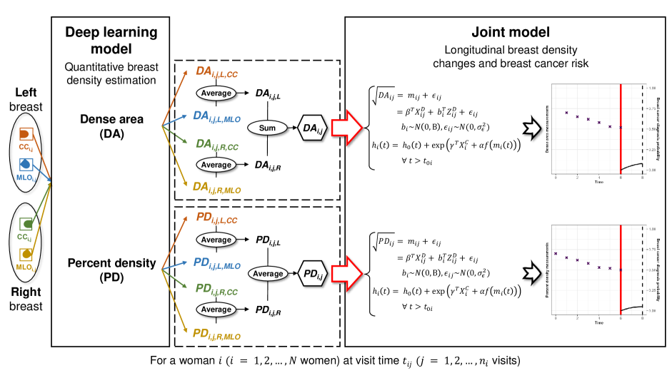
Figure 1: The DeepJoint algorithm pipeline

4 Results

4.1 The deep learning model

Table 2 displays the DSCs derived from the left-out test set comprising 84 images from 21 women. The model exhibited a satisfactory performance overall, with an average DSC of 0.993 for breast and 0.848 for dense areas on the test set. In addition, results showed the model’s adequate performance regarding breast and dense DSC values, regardless of the view, manufacturer, or screening center. Across all BI-RADS score categories, breast DSC results remained consistently high, while some variability was noted for dense DSC, particularly in the A class, although still within acceptable limits.

Table 2: Mean (standard deviation) of breast and dense Dice-Sorensen coefficients (DSC) obtained on the test set (N = 84 images)

Performance on the test set
Variable	Breast DSC	Dense DSC
All data	0.993 ($\pm$0.007)	0.848 ($\pm$0.118)
Center
1	0.993 ($\pm$0.008)	0.845 ($\pm$0.121)
2	0.993 ($\pm$0.006)	0.859 ($\pm$0.110)
Manufacturer
Hologic	0.993 ($\pm$0.006)	0.849 ($\pm$0.122)
GEHC	0.993 ($\pm$0.009)	0.847 ($\pm$0.113)
BI-RADS score
A	0.995 ($\pm$0.006)	0.675 ($\pm$0.094)
B	0.991 ($\pm$0.008)	0.841 ($\pm$0.052)
C	0.994 ($\pm$0.004)	0.916 ($\pm$0.028)
D	0.990 ($\pm$0.010)	0.947 ($\pm$0.022)
View
CC	0.996 ($\pm$0.004)	0.840 ($\pm$0.130)
MLO	0.990 ($\pm$0.009)	0.857 ($\pm$0.105)

4.2 The joint model

We calculated the quantitative breast density metrics for the 77,298 women in our dataset. Baseline dense area estimates ranged from 0 to 459.05 $cm^{2}$, with median values of 77.9 [44.3 - 114.8] $cm^{2}$ in cancer-free individuals and 92.2 [55.8 - 127.9] $cm^{2}$ in the cancer group. On the other hand, baseline percent density estimates varied from 0 to 93.3% with medians of 34.5 [16.0 - 50.0] % and 37.0 [20.1 - 49.6] % in cancer-free and cancer groups, respectively. Baseline estimates of dense area and percent density according to baseline BI-RADS scores are reported in Appendix Table A.1. Our deep learning model yielded adequate quantitative breast density evaluations for each BI-RADS density, categorizing them into four distinct groups. Women diagnosed with breast cancer consistently exhibited higher median values compared to those without breast cancer, except for median percent density values in C and D classes. Although there was a discernible difference, percent density assessments in these classes remained very close.
We fitted two distinct types of joint models, each using one of the two longitudinal biomarkers ($Y_{i}$ is either dense area or percent density). To ensure the biomarkers’ normality, the square root transformation was applied. Appendix Figure A.3 displays the square root of the longitudinal biomarkers measurements for 1000 randomly selected women, connected by lines. Using a natural cubic spline, data points were smoothed and represented by the red curve with 95% confidence bands illustrated in black. Overall, both biomarkers seem to decrease with age as previously described in the literature [Lokate et al. 2013]. In the joint model, we addressed delayed entry and left truncation by introducing an adjustment on age as explained in section 2.2.1. Additionally, we considered the age at the first screening visit ($age_{0}$) and the manufacturer ($manuf$) as additional factors in the longitudinal sub-model. We evaluated four link functions, as reported in equations  3,  4,  5 and 6. Results for all fitted joint models are presented in Table 3.

$$\left\{\begin{array}[]{ll}\sqrt{Y_{ij}}&=m_{ij}+\epsilon_{ij}\\[2.84544pt] &=(\beta_{0}+b_{i0})+(\beta_{1}+b_{i1})\ age_{ij}+\beta_{2}\ age_{0i}+\ \beta_{3}\ manuf_{i}+\epsilon_{ij}\\[5.69046pt] h_{i}(age)&=h_{0}(age)\ exp\Big{\{}\alpha\ f(m_{i}(age))\Big{\}}\\[5.69046pt] \end{array}\right.$$ (10)

Table 3: Estimated posterior means and 95% credible intervals for the joint models’ coefficients, fitted to a dataset of $N=77,298$ screened women, employing as link function the current level (Model 1), the current slope (Model 2), the current level and slope (Model 3), or the cumulative level (Model 4) of the longitudinal biomarker (dense area or percent density)

	JM with $\bm{\sqrt{dense\ area\ (cm^{2})}}$			JM with $\bm{\sqrt{percent\ density\ (\%)}}$
Coefficient	Mean	95$\%$CI	$\hat{R}$	Mean	95$\%$CI	$\hat{R}$
Model 1
Longitudinal sub-model
Intercept ($\beta_{0}$)	9.135	(8.839, 9.432)	1.006	6.408	(6.207, 6.612)	1.002
Age ($\beta_{1}$)	-0.114	(-0.118, -0.111)	1.029	-0.081	(-0.084, -0.079)	1.002
$Age_{0}$ ($\beta_{2}$)	0.017	(0.012, 0.023)	1.013	0.000	(-0.004, 0.004)	1.006
$Manuf.^{*}$ ($\beta_{3}$)	0.163	(0.145, 0.182)	1.022	0.184	(0.172, 0.196)	1.035
$\sigma_{\epsilon}$	0.603	(0.599, 0.606)	1.002	0.375	(0.373, 0.377)	1.003
Survival Sub-model
Current level ($\alpha_{1}$)	0.109	(0.051, 0.166)	1.000	0.125	(0.033, 0.219)	1.003
DIC	82,092.46			58,329.67
Model 2
Longitudinal sub-model
Intercept ($\beta_{0}$)	9.144	(8.846, 9.440)	1.004	6.412	(6.214, 6.611)	1.001
Age ($\beta_{1}$)	-0.114	(-0.117, -0.111)	1.025	-0.081	(-0.084, -0.079)	1.021
$Age_{0}$ ($\beta_{2}$)	0.017	(0.011, 0.023)	1.010	0.000	(-0.004, 0.004)	1.004
$Manuf.^{*}$ ($\beta_{3}$)	0.161	(0.142, 0.181)	1.041	0.184	(0.172, 0.196)	1.035
$\sigma_{\epsilon}$	0.603	(0.599, 0.607)	1.003	0.375	(0.373, 0.377)	1.006
Survival Sub-model
Current slope ($\alpha_{2}$)	0.038	(0.004, 0.063)	1.003	0.033	(0.006, 0.053)	1.013
DIC	82,097.67			58,326.79
Model 3
Longitudinal sub-model
Intercept ($\beta_{0}$)	9.155	(8.857, 9.453)	1.009	6.410	(6.213, 6.608)	1.007
Age ($\beta_{1}$)	-0.114	(-0.118, -0.110)	1.022	-0.082	(-0.084, -0.079)	1.019
$Age_{0}$ ($\beta_{2}$)	0.017	(0.011, 0.023)	1.013	0.000	(-0.003, 0.004)	1.011
$Manuf.^{*}$ ($\beta_{3}$)	0.162	(0.143, 0.181)	1.009	0.184	(0.172, 0.195)	1.005
$\sigma_{\epsilon}$	0.603	(0.599, 0.607)	1.056	0.375	(0.373, 0.378)	1.076
Survival Sub-model
Current level ($\alpha_{1}$)	0.116	(0.056, 0.174)	1.002	0.134	(0.041, 0.228)	1.005
Current slope ($\alpha_{2}$)	0.042	(0.019, 0.062)	1.003	0.038	(0.018, 0.053)	1.004
DIC	82,070.83			58,304.56
Model 4
Longitudinal sub-model
Intercept ($\beta_{0}$)	9.147	(8.849, 9.447)	1.000	6.414	(6.214, 6.611)	1.002
Age ($\beta_{1}$)	-0.114	(-0.118, -0.111)	1.002	-0.081	(-0.084, -0.079)	1.002
$Age_{0}$ ($\beta_{2}$)	0.017	(0.011, 0.023)	1.001	0.000	(-0.003, 0.004)	1.004
$Manuf.^{*}$ ($\beta_{3}$)	0.163	(0.144, 0.182)	1.012	0.184	(0.172, 0.196)	1.011
$\sigma_{\epsilon}$	0.603	(0.599, 0.606)	1.016	0.375	(0.372, 0.377)	1.003
Survival Sub-model
Cumulative level ($\alpha_{3}$)	0.125	(0.064, 0.184)	1.001	0.149	(0.054, 0.245)	1.002
DIC	82,093.73			58,328.89
$Manuf.^{*}$: Hologic vs. GEHC manufacturer
JM: Joint model; CI: Credible interval; DIC: Deviance information criterion
Bold DIC represent the best joint model

All the fitted joint models exhibited satisfactory convergence properties with $\hat{R}<1.10$ for all coefficients. Regardless of the biomarker, the model with the current level and slope of the biomarker’s trajectory at a given age demonstrated the best fit according to the DIC values (Model 3: dense area, DIC = 82,070.83; percent density, DIC = 58,304.56). Results were consistent across all models, indicating a negative association between the longitudinal biomarker and age, aligning with existing literature and the observed trends in Appendix Figure A.3. The association between the longitudinal biomarker and the age at the first screening visit ($age_{0}$) varied depending on the biomarker: a positive association was observed for dense area across all models, while no association was observed for percent density across all models. Additionally, a positive association was identified between the longitudinal biomarker and Hologic manufacturers, regardless of the biomarker type. In the survival sub-model, a positive association was observed between the longitudinal dense area’s current level and slope and the risk of breast cancer, with coefficients of 0.116 ($95\%$ credible interval (CI): 0.056, 0.174) and 0.042 (0.019, 0.062), respectively. Similar patterns were observed in the joint model incorporating percent density as the longitudinal biomarker, where the current level and slope of the biomarker’s trajectory were positively associated with the risk of breast cancer, yielding coefficients of 0.134 (0.041, 0.228) and 0.038 (0.018, 0.053), respectively. These findings imply that elevated levels of quantitative breast density at a given age are linked to a higher risk of breast cancer. Furthermore, in the context of a continuous decrease in quantitative breast density over time, women with a slower decrease (i.e. a negative slope close to zero) in their biomaker’s level are more prone to breast cancer risk compared to those with a faster decrease (i.e. a negative slope far from zero), assuming similar levels of the biomarker at a specific age. Consistent trends were also noted in Models 1 and 2 (Table 3) where either the current value or the current slope of the longitudinal biomarker were incorporated in the survival sub-model, mirroring the outcomes of the best model. Additionally, Model 4, employing the cumulative breast density level up to a definite age as a link function, also demonstrated a positive association between the cumulative breast density level and the risk of breast cancer.

4.3 Individual and dynamic breast cancer risk prediction

Individual and dynamic breast cancer risk predictions for the next five years were computed using the optimal joint model (Model 3, Table 3). We illustrate the results for 24 randomly selected women who started screening at ages 42, 54, or 65, assessing their 5-year breast cancer risk at landmark times corresponding to different age ranges for each group ($45-49$, $58-62$, and $68-72$ years, respectively). Results for the group of women starting their screening at age 54 are presented in Figure 2, and other group’s figures are provided in the Appendix. Comparing age groups, breast cancer risk seemed to increase with age for women with similar dense area or percent density profiles (example: Subjects 14, 5, and 12 in Figure 2 and Appendix Figures A.4 and A.5, respectively). Within an age group, women with consistently high breast density levels over time exhibited higher 5-year breast cancer risks, coherent with results in Table 3. Also, individual 5-year breast cancer risk probabilities differed when using either dense area or percent density as the longitudinal biomarker for some women (example: Subject 18 in Figure 2). We also computed individual 2-year breast cancer risk predictions for all groups to align with screening visit frequencies, yielding similar results (Appendix).

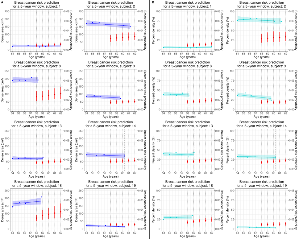
Figure 2: Individual breast cancer risk predictions for the next five years at landmark times ranging from $58$ to $62$ years for eight randomly selected women starting screening at the age of 54 years. Predictions were generated using the optimal joint model with either dense area (Panel A) or percent density (Panel B) as the longitudinal biomarker. Blue and cyan dots represent the observed dense area and percent density evaluations, respectively. Blue and cyan bold lines illustrate the joint model’s subject-specific longitudinal profiles for dense area and percent density, respectively, along with their corresponding 95% credible intervals. Black dotted lines indicate landmark times, while black dashed lines represent breast cancer occurrence, if any. Red squares and bands denote the mean 5-year breast cancer risk probabilities and their 95% credible intervals. These predictions are based on the biomarker’s evaluations up to a given landmark time, excluding subsequent observations (Example: For subject 14, the last observation after age 60 is excluded when calculating the 5-year breast cancer risk at landmark time 60 years. However, it is included, along with the other observations, for probability calculation at landmark time 61)

Next, we assessed the predictive performance of Model 3 (Table 3) when considering dense area or percent density as the longitudinal biomarker using AUC and BS. Evaluation considered breast cancer risk predictions at landmark times $s=\{41,42,...,65\}$ and a fixed prediction window of $w=5$ years. Comparing the two joint models, we reported the $\Delta(AUC)$ and $\Delta(BS)$, representing the differences in AUC and BS between the model with percent density versus the one with dense area. Results in Figure 3 showed similar discrimination ability with a slight advantage for the joint model with dense area, though statistically insignificant as 0 was into the $95\%$ confidence interval of $\Delta(AUC)$. Models’ calibration was comparable, with $\Delta(BS)$ values close to zero. Similar trends were observed for a fixed prediction window of $w=2$ years (Appendix).

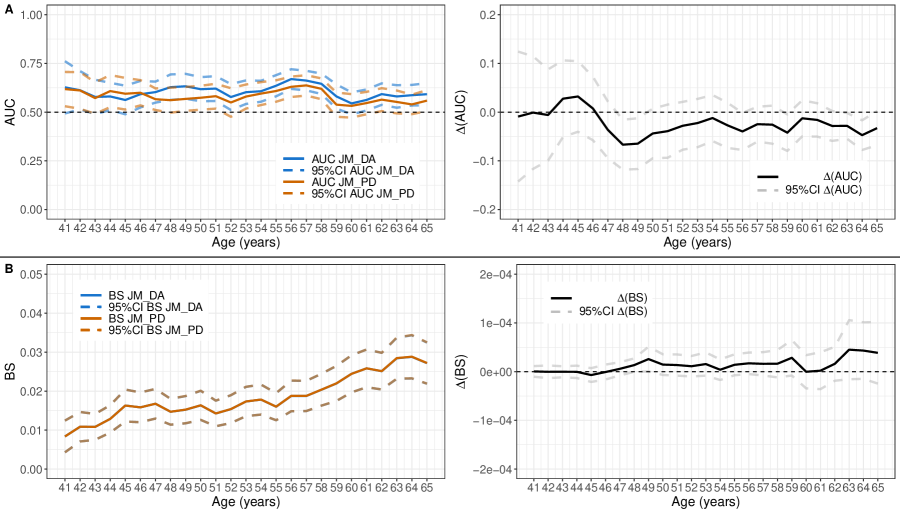
Figure 3: Comparison of the predictive accuracy of breast cancer risk using the optimal joint model (JM) with either dense area (DA) or percent density (PD) as the longitudinal biomarker within time window $(s,s+w)$ when $s=\{41,42,...,65\}$ and $w=5$ years. $\Delta(AUC)$ and $\Delta(BS)$ denote the differences in AUC and BS between JM with PD versus JM with DA. Dashed lines represent $95\%$ point-wise confidence intervals (CIs).

5 Discussion

In this study, we introduced the DeepJoint algorithm, an open-source pipeline for quantitative breast density evaluation, coupled with the assessment of its longitudinal evolution and its impact on the risk of breast cancer in women undergoing screening from the age of 40 onward. Individual and dynamic breast cancer risk predictions were also derived, offering a personalized assessment of the risk.
The deep learning component of the DeepJoint algorithm involved a fine-tuning step of MammoDL [Muthukrishnan et al. 2022], accompanied by script modifications to enhance user-friendliness and simplicity. This fine-tuning process was executed on 832 images from 208 women with available reference breast and dense segmentation masks. Leveraging a pre-trained model on a large and multi-institutional dataset in addition to the implementation of a 10-fold cross-validation step, our results, obtained on a moderately sized dataset, were satisfactory on the left-out test set. Our ability to include more women was constrained by the challenges associated with the time-consuming and labor-intensive process of generating reference masks. Nevertheless, the final version of our deep learning model provided visit-level breast density assessments that aligned with BI-RADS evaluations (Appendix Table A.1).
Besides, the goodness-of-fit of four distinct joint models, differentiated by the function linking the longitudinal biomarker with the risk of breast cancer, was assessed using an extensive dataset of $77,298$ women. We overcame the challenge of fitting a joint model to such a substantial dataset by employing Bayesian inference and the consensus Monte Carlo algorithm [Afonso et al. 2023]. The best joint model, regardless of the biomarker type, incorporated both the current value and slope of the longitudinal biomarker at a specified age. This model showed a positive association between the age at the first screening visit and the longitudinal dense area, implying higher breast density in women starting their screening at an older age. However, this association was not observed when using the percent density. This discrepancy might be linked to an underlying population selection process, suggesting factors beyond age heterogeneity influencing these results. Besides, the best model demonstrated a positive association between the current level and slope of both longitudinal biomarkers and the risk of breast cancer. These findings suggest that higher levels of quantitative breast density are linked to an increased risk of breast cancer and that although breast density tends to regress with age, women with no to little decrease in breast density with age are more likely to be at risk for breast cancer compared to those with a faster decrease. Our observations are consistent with [Ghosh et al. 2010]’s work, where they showed that the absence of lobular involution, indicating no age-related atrophy of breast lobules, is associated with a higher breast cancer risk. This risk is amplified when the absence of involution is combined with high breast density. Additionally, our results align with those in [Illipse et al. 2023], except for the association between the biomarker’s current slope and the risk of breast cancer, possibly due to differences in the biomarker definition, lack of adjustment variables in our joint model, and cohorts variations. We also derived individual and dynamic breast cancer risk probabilities for 2- and 5-year windows, and showed variations in risk estimations when using dense area or percent density as the longitudinal biomarker. This demonstrates the distinct information each metric provides, emphasizing the need for their mutual exploration. In addition, the versatility in selecting prediction time frames accommodates various clinical queries, whether the focus is on long-term risk prediction or close risk monitoring. Although our dataset lacks additional breast cancer risk factors, our methodology is well-suited for their inclusion as adjustment variables. This adaptability stands out as a strength, aligning with the growing emphasis on tailoring personalized screening guidelines [Roux et al. 2022].
Besides breast density, various mammographic textures hold the potential to refine breast cancer risk estimation. [Jiang et al. 2023] emphasized the significance of considering additional image-based features alongside breast density to enhance breast cancer prediction during screening by presenting appropriate methodologies for dimension reduction from imaging data when interested in a time-to-event outcome. In future work, we aim to explore the effect of image-based features and integrate them into the joint model framework. This incorporation is possible either in the longitudinal sub-model, offering a comprehensive description of dense tissue distribution in the breast, or in the survival sub-model. This exploration will assess how these features, alongside the longitudinal evolution of quantitative breast density, influence breast cancer risk.
In addition to FFDM, digital breast tomosynthesis (DBT) has demonstrated promising results in breast cancer detection within the screening setting. A 2-dimensional reconstruction of the DBT slices generates 2D synthetic mammography (2DSM) images without additional radiation exposure, offering a notable advantage for women participating regularly in screening. In previous investigations, [Conant et al. 2017] have established agreement between breast density assessments from FFDM and 2DSM. Consequently, alongside FFDM images, we intend to assess our model’s performance on 2DSM images, expanding its application scope. Lastly, [Dadsetan et al. 2022] explored a full deep learning methodology for breast cancer assessment, by capturing spatiotemporal changes in bilateral breast tissue features. While this approach holds promise, multiple challenges constraints its practical implementation, including necessity for a substantial dataset, incompatibility with varying visit numbers and intervals, and limited interpretability attributed to the ”black-box” nature.

Additional information

Appendix A: Predictive accuracy measures

Dynamic AUC

The AUC assesses the discrimination ability of a predictive tool, with higher values indicating the tool’s capacity to give higher predicted risks of event for subjects who are more likely to experience the event than for subjects who are less likely to experience it. Let $D(s,w)$ be the observed outcome in a specific time span $[s,s+w]$ in women still at risk at time $s$. Given that $D(s,w)$ is not always observable in the presence of right-censored data, we define $\tilde{D}(s,w)=\mathds{1}_{s<T<s+w}$, that equals $1$ when the event of interest occurs within $[s,s+w]$, and $0$ otherwise. To handle right-censored data, the dynamic AUC is estimated using the the Inverse Probability of Censoring Weighting (IPCW) method. As a result, the expected AUC at a landmark time $s$ for a fixed prediction window $w$ is given by

$$\begin{array}[]{ll}\displaystyle AUC(s,w)&=\mathrm{P}\Big{(}\pi_{i}(s+w)>\pi_{j}^{*}(s+w)|D_{i}(s,w)=1,\ D_{j}(s,w)=0,\ T_{i}>s,\ T_{j}>s\Big{)}\\[8.5359pt] &=\frac{\sum_{i=1}^{N}\sum_{j=1}^{N}\ \mathds{1}_{(\pi_{i}(s+w)>\pi_{j}^{*}(s+w))}\ \tilde{D_{i}}(s,w)\ (1-\tilde{D_{j}}(s,w))\ \widehat{W_{i}}(s,w)\ \widehat{W_{j}}(s,w)}{\sum_{i=1}^{N}\sum_{j=1}^{N}\ \tilde{D_{i}}(s,w)\ (1-\tilde{D_{j}}(s,w))\ \widehat{W_{i}}(s,w)\ \widehat{W_{j}}(s,w)}\end{array}$$ (11)

here, $\widehat{W_{i}}(s,w)$ are weights to account for right-censoring, defined as

$$\begin{array}[]{ll}\displaystyle\widehat{W_{i}}(s,w)&=\frac{\mathds{1}_{(T_{i}>s+w)}}{\tilde{G}(s+w|s)}+\frac{\mathds{1}_{(s<T_{i}<s+w)}\delta_{i}}{\tilde{G}(T_{i}|s)}\\ \end{array}$$ (12)

with $\hat{G(u)}$ as the Kaplan-Meier estimator of the survival function at censoring time $u$, such as $\forall u>s$, $\hat{G}(u|s)=\hat{G}(u)/\hat{G}(s)$.

Dynamic Brier score

The Brier score represents the mean squared error between predicted probabilities $\pi(s+w)$ at a given time $s+w$ and the observed outcome $D(s,w)$ in women still at risk at time $s$. Consequently, the lower and closest to zero is the BS, the better. Dynamic BS, accounting for right-censoring, is estimated using the IPCW method. The expected BS at a horizon time $s+w$ is defined as

$$\begin{array}[]{ll}\displaystyle BS(s,w)&=\mathit{E}\Big{[}(D(s,w)-\pi_{i}(s+w))^{2}|T>s\Big{]}\\ &=\frac{1}{\sum_{i=1}^{N}\mathds{1}_{T_{i}>s}}\sum_{i=1}^{N}\widehat{W_{i}}(s,w)\Big{(}\tilde{D_{i}}(s,w)-\pi_{i}(s+w)\Big{)}^{2}\\ \end{array}$$ (13)

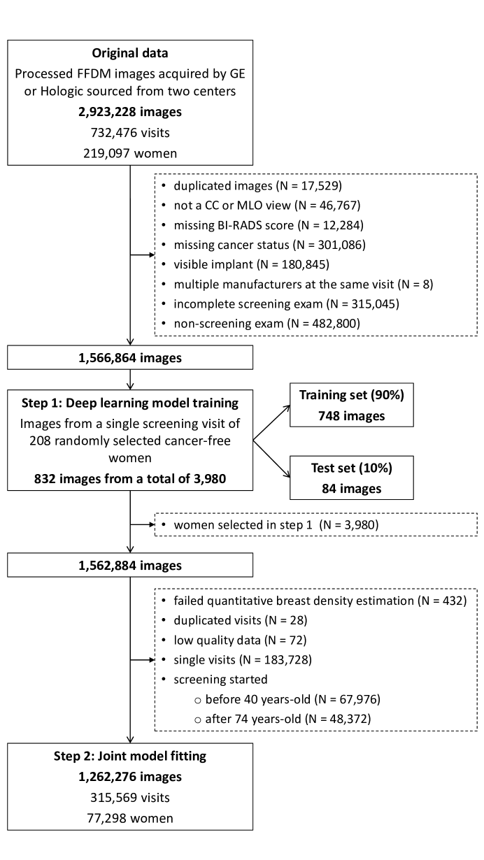
Figure A.1: Data flowchart. Numbers are for images unless specified. Dashed boxes correspond to eliminated data

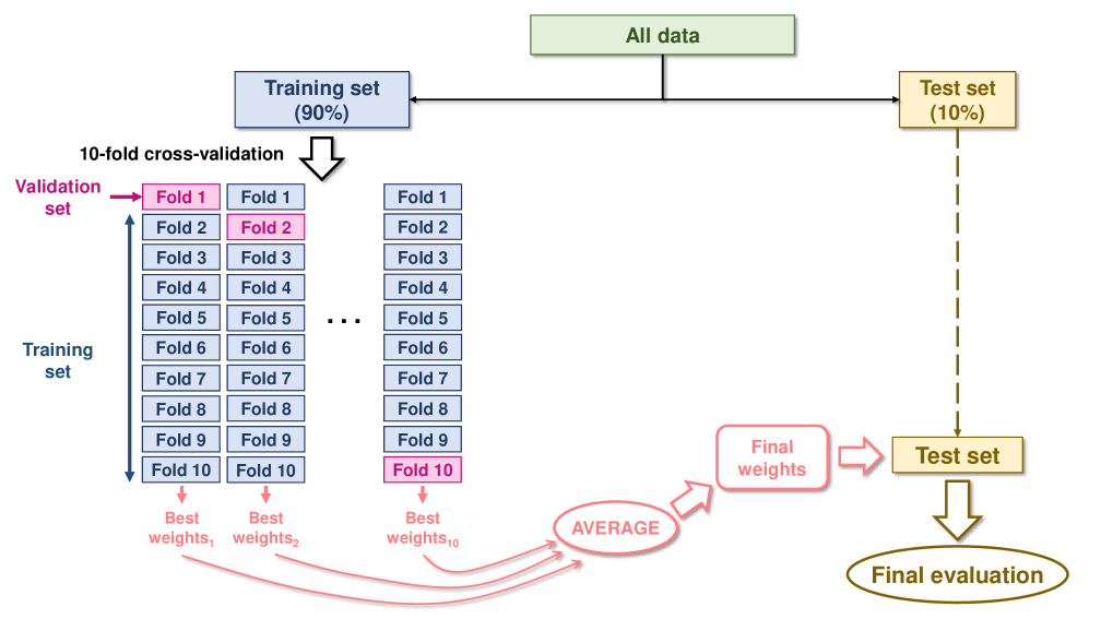
Figure A.2: The training process of the DeepJoint algorithm’s deep learning component using 10-fold cross-validation

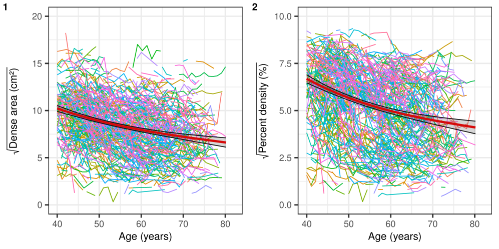
Figure A.3: The square root of (1) dense area (in $cm^{2}$) and (2) percent density (in %) measurements according to age for 1000 randomly selected women with the smoothed average (in red) and the 95% confidence bands (in black)

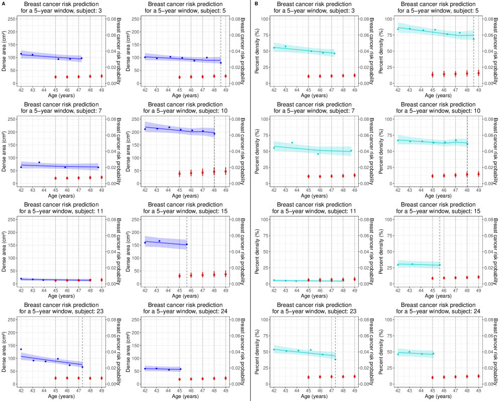
Figure A.4: Individual breast cancer risk predictions for the next five years at landmark times ranging from $45$ to $49$ years for eight randomly selected women starting screening at the age of 42 years. Predictions were generated using the optimal joint model with either dense area (Panel A) or percent density (Panel B) as the longitudinal biomarker. Blue and cyan dots represent the observed dense area and percent density evaluations, respectively. Blue and cyan bold lines illustrate the joint model’s subject-specific longitudinal profiles for dense area and percent density, respectively, along with their corresponding 95% credible intervals. Black dotted lines indicate landmark times, while black dashed lines represent breast cancer occurrence, if any. Red squares and bands denote the mean 5-year breast cancer risk probabilities and their 95% credible intervals. These predictions are based on the biomarker’s evaluations up to a given landmark time, excluding subsequent observations (Example: For subject 5, the last observation past age 48 is excluded when calculating the 5-year breast cancer risk at landmark time 48 years. However, it is included, along with the other observations, for probability calculation at landmark time 49)

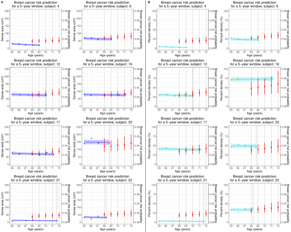
Figure A.5: Individual breast cancer risk predictions for the next five years at landmark times ranging from $68$ to $72$ years for eight randomly selected women starting screening at the age of 65 years. Predictions were generated using the optimal joint model with either dense area (Panel A) or percent density (Panel B) as the longitudinal biomarker. Blue and cyan dots represent the observed dense area and percent density evaluations, respectively. Blue and cyan bold lines illustrate the joint model’s subject-specific longitudinal profiles for dense area and percent density, respectively, along with their corresponding 95% credible intervals. Black dotted lines indicate landmark times, while black dashed lines represent breast cancer occurrence, if any. Red squares and bands denote the mean 5-year breast cancer risk probabilities and their 95% credible intervals. These predictions are based on the biomarker’s evaluations up to a given landmark time, excluding subsequent observations (Example: For subject 16, the last observation past age 71 is excluded when calculating the 5-year breast cancer risk at landmark time 71 years. However, it is included, along with the other observations, for probability calculation at landmark time 72)

Figure A.6: Individual breast cancer risk predictions for the next two years at landmark times ranging from $45$ to $49$ years for eight randomly selected women starting screening at the age of 42 years. Predictions were generated using the optimal joint model with either dense area (Panel A) or percent density (Panel B) as the longitudinal biomarker. Blue and cyan dots represent the observed dense area and percent density evaluations, respectively. Blue and cyan bold lines illustrate the joint model’s subject-specific longitudinal profiles for dense area and percent density, respectively, along with their corresponding 95% credible intervals. Black dotted lines indicate landmark times, while black dashed lines represent breast cancer occurrence, if any. Red squares and bands denote the mean 2-year breast cancer risk probabilities and their 95% credible intervals. These predictions are based on the biomarker’s evaluations up to a given landmark time, excluding subsequent observations (Example: For subject 5, the last observation past age 48 is excluded when calculating the 2-year breast cancer risk at landmark time 48 years. However, it is included, along with the other observations, for probability calculation at landmark time 49)

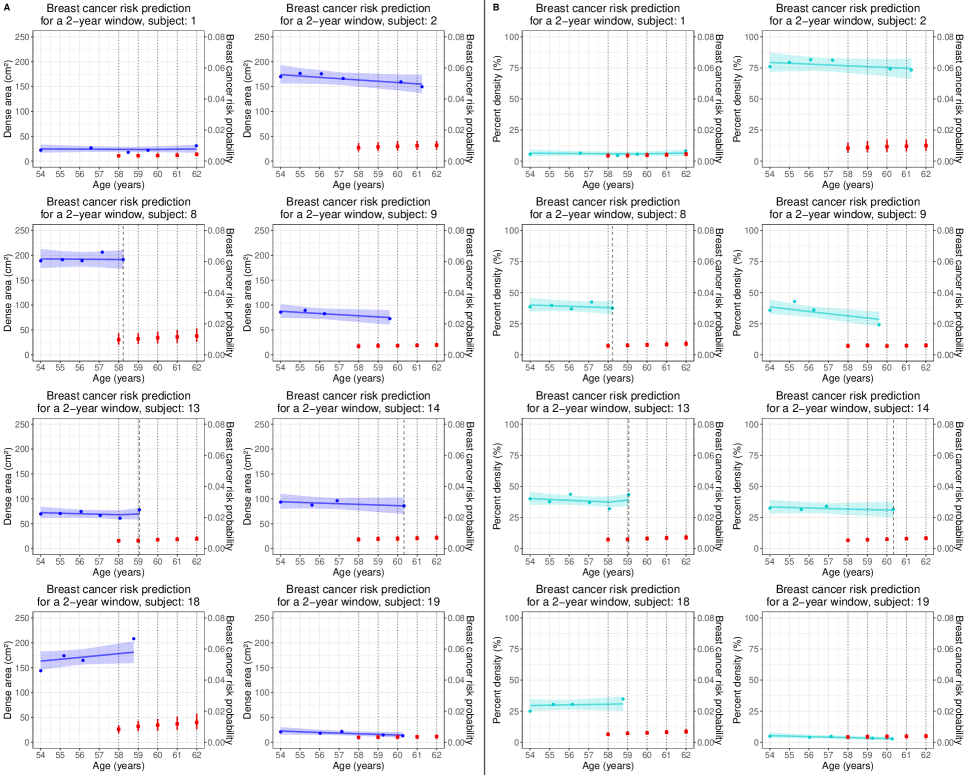
Figure A.7: Individual breast cancer risk predictions for the next two years at landmark times ranging from $58$ to $62$ years for eight randomly selected women starting screening at the age of 54 years. Predictions were generated using the optimal joint model with either dense area (Panel A) or percent density (Panel B) as the longitudinal biomarker. Blue and cyan dots represent the observed dense area and percent density evaluations, respectively. Blue and cyan bold lines illustrate the joint model’s subject-specific longitudinal profiles for dense area and percent density, respectively, along with their corresponding 95% credible intervals. Black dotted lines indicate landmark times, while black dashed lines represent breast cancer occurrence, if any. Red squares and bands denote the mean 2-year breast cancer risk probabilities and their 95% credible intervals. These predictions are based on the biomarker’s evaluations up to a given landmark time, excluding subsequent observations (Example: For subject 14, the last observation after age 60 is excluded when calculating the 2-year breast cancer risk at landmark time 60 years. However, it is included, along with the other observations, for probability calculation at landmark time 61)

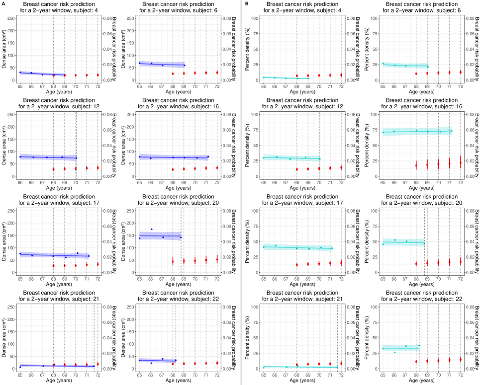
Figure A.8: Individual breast cancer risk predictions for the next two years at landmark times ranging from $68$ to $72$ years for eight randomly selected women starting screening at the age of 65 years. Predictions were generated using the optimal joint model with either dense area (Panel A) or percent density (Panel B) as the longitudinal biomarker. Blue and cyan dots represent the observed dense area and percent density evaluations, respectively. Blue and cyan bold lines illustrate the joint model’s subject-specific longitudinal profiles for dense area and percent density, respectively, along with their corresponding 95% credible intervals. Black dotted lines indicate landmark times, while black dashed lines represent breast cancer occurrence, if any. Red squares and bands denote the mean 2-year breast cancer risk probabilities and their 95% credible intervals. These predictions are based on the biomarker’s evaluations up to a given landmark time, excluding subsequent observations (Example: For subject 16, the last observation past age 71 is excluded when calculating the 2-year breast cancer risk at landmark time 71 years. However, it is included, along with the other observations, for probability calculation at landmark time 72)

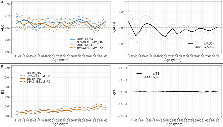
Figure A.9: Comparison of the predictive accuracy of breast cancer risk using the optimal joint model (JM) with either dense area (DA) or percent density (PD) as the longitudinal biomarker within time window $(s,s+w)$ when $s=\{41,42,...,65\}$ and $w=2$ years. $\Delta(AUC)$ and $\Delta(BS)$ denote the differences in AUC and BS between JM with PD versus JM with DA. Dashed lines represent $95\%$ point-wise confidence intervals (CIs)

Table A.1: Visit-level dense area and percent density evaluations based on the deep learning component of the DeepJoint algorithm according to BI-RADS scores for $N=77,298$ screened women

	BI-RADS score
	A	B	C	D
At baseline	N = 9,034	N = 27,988	N = 32,753	N = 7,523
Dense area $(cm^{2})$
Cancer-free	19.3 [10.1 - 35.3]	59.0 [35.5 - 89.4]	98.8 [72.2 - 131.6]	114.2 [86.4 - 151.0]
Cancer	21.0 [14.5 - 38.6]	65.2 [41.9 - 98.5]	108.1 [84.2 - 141.0]	122.6 [98.7 - 150.5]
Percent density $(\%)$
Cancer-free	4.9 [2.5 - 10.0]	21.4 [11.4 - 33.7]	44.5 [34.3 - 54.3]	62.3 [53.2 - 71.6]
Cancer	5.0 [4.5 - 9.5]	22.4 [12.6 - 36.3]	43.6 [33.8 - 52.7]	59.3 [51.3 - 69.4]
Data are median [IQR]

References

- [Afonso et al. 2023] Afonso, P. M., Rizopoulos, D., Palipana, A. K., Zhou, G. C., Brokamp, C., Szczesniak, R. D., and Andrinopoulou, E.-R. (2023). Efficiently analyzing large patient registries with Bayesian joint models for longitudinal and time-to-event data. arXiv:2310.03351 [stat].
- [Armero et al. 2016] Armero, C., Forné, C., Rué, M., Forte, A., Perpiñán, H., Gómez, G., and Baré, M. (2016). Bayesian joint ordinal and survival modeling for breast cancer risk assessment. Statistics in Medicine 35, 5267–5282.
- [Blanche et al. 2015] Blanche, P., Proust-Lima, C., Loubère, L., Berr, C., Dartigues, J.-F., and Jacqmin-Gadda, H. (2015). Quantifying and comparing dynamic predictive accuracy of joint models for longitudinal marker and time-to-event in presence of censoring and competing risks. Biometrics 71, 102–113.
- [Boyd et al. 2018] Boyd, N., Berman, H., Zhu, J., Martin, L. J., Yaffe, M. J., Chavez, S., Stanisz, G., Hislop, G., Chiarelli, A. M., Minkin, S., and Paterson, A. D. (2018). The origins of breast cancer associated with mammographic density: a testable biological hypothesis. Breast Cancer Research 20, 1–13. Number: 1 Publisher: BioMed Central.
- [Checka et al. 2012] Checka, C. M., Chun, J. E., Schnabel, F. R., Lee, J., and Toth, H. (2012). The Relationship of Mammographic Density and Age: Implications for Breast Cancer Screening. American Journal of Roentgenology 198, W292–W295. Publisher: American Roentgen Ray Society.
- [Conant et al. 2017] Conant, E. F., Keller, B. M., Pantalone, L., Gastounioti, A., McDonald, E. S., and Kontos, D. (2017). Agreement between Breast Percentage Density Estimations from Standard-Dose versus Synthetic Digital Mammograms: Results from a Large Screening Cohort Using Automated Measures. Radiology 283, 673–680.
- [Dadsetan et al. 2022] Dadsetan, S., Arefan, D., Berg, W. A., Zuley, M. L., Sumkin, J. H., and Wu, S. (2022). Deep learning of longitudinal mammogram examinations for breast cancer risk prediction. Pattern recognition 132, 108919.
- [Dembrower et al. 2020] Dembrower, K., Liu, Y., Azizpour, H., Eklund, M., Smith, K., Lindholm, P., and Strand, F. (2020). Comparison of a Deep Learning Risk Score and Standard Mammographic Density Score for Breast Cancer Risk Prediction. Radiology 294, 265–272. Publisher: Radiological Society of North America.
- [Dice 1945] Dice, L. R. (1945). Measures of the Amount of Ecologic Association Between Species. Ecology 26, 297–302. _eprint: https://onlinelibrary.wiley.com/doi/pdf/10.2307/1932409.
- [Falcon and The PyTorch Lightning team 2019] Falcon, W. and The PyTorch Lightning team (2019). https://github.com/Lightning-AI/lightning
- [Ghosh et al. 2010] Ghosh, K., Vachon, C. M., Pankratz, V. S., Vierkant, R. A., Anderson, S. S., Brandt, K. R., Visscher, D. W., Reynolds, C., Frost, M. H., and Hartmann, L. C. (2010). Independent Association of Lobular Involution and Mammographic Breast Density With Breast Cancer Risk. JNCI: Journal of the National Cancer Institute 102, 1716–1723.
- [Gudhe et al. 2022] Gudhe, N. R., Behravan, H., Sudah, M., Okuma, H., Vanninen, R., Kosma, V.-M., and Mannermaa, A. (2022). Area-based breast percentage density estimation in mammograms using weight-adaptive multitask learning. Scientific Reports 12, 12060. Number: 1 Publisher: Nature Publishing Group.
- [Haars et al. 2005] Haars, G., van Noord, P. A. H., van Gils, C. H., Grobbee, D. E., and Peeters, P. H. M. (2005). Measurements of breast density: no ratio for a ratio. Cancer Epidemiology, Biomarkers & Prevention: A Publication of the American Association for Cancer Research, Cosponsored by the American Society of Preventive Oncology 14, 2634–2640.
- [Haji Maghsoudi et al. 2021] Haji Maghsoudi, O., Gastounioti, A., Scott, C., Pantalone, L., Wu, F.-F., Cohen, E. A., Winham, S., Conant, E. F., Vachon, C., and Kontos, D. (2021). Deep-LIBRA: An artificial-intelligence method for robust quantification of breast density with independent validation in breast cancer risk assessment. Medical Image Analysis 73, 102138.
- [ Hartman et al. 2008] Hartman, K., Highnam, R., Warren, R., and Jackson, V. (2008). Volumetric Assessment of Breast Tissue Composition from FFDM Images. In Krupinski, E. A., editor, Digital Mammography, Lecture Notes in Computer Science, pages 33–39, Berlin, Heidelberg. Springer.
- [Highnam et al. 2010] Highnam, R., Brady, S. M., Yaffe, M. J., Karssemeijer, N., and Harvey, J. (2010). Robust Breast Composition Measurement - VolparaTM. In Martí, J., Oliver, A., Freixenet, J., and Martí, R., editors, Digital Mammography, Lecture Notes in Computer Science, pages 342–349, Berlin, Heidelberg. Springer.
- [Illipse et al. 2023] Illipse, M., Czene, K., Hall, P., and Humphreys, K. (2023). Studying the association between longitudinal mammographic density measurements and breast cancer risk: a joint modelling approach. Breast cancer research: BCR 25, 64.
- [Jiang et al. 2023] Jiang, S., Bennett, D. L., Rosner, B. A., and Colditz, G. A. (2023). Longitudinal Analysis of Change in Mammographic Density in Each Breast and Its Association With Breast Cancer Risk. JAMA Oncology .
- [Jiang et al. 2023] Jiang, S., Cao, J., Rosner, B., and Colditz, G. A. (2023). Supervised two-dimensional functional principal component analysis with time-to-event outcomes and mammogram imaging data. Biometrics 79, 1359–1369. _eprint: https://onlinelibrary.wiley.com/doi/pdf/10.1111/biom.13611.
- [Keller et al. 2012] Keller, B. M., Nathan, D. L., Wang, Y., Zheng, Y., Gee, J. C., Conant, E. F., and Kontos, D. (2012). Estimation of breast percent density in raw and processed full field digital mammography images via adaptive fuzzy c-means clustering and support vector machine segmentation. Medical Physics 39, 4903–4917. _eprint: https://aapm.onlinelibrary.wiley.com/doi/pdf/10.1118/1.4736530.
- [Król et al. 2016] Król, A., Ferrer, L., Pignon, J.-P., Proust-Lima, C., Ducreux, M., Bouché, O., Michiels, S., and Rondeau, V. (2016). Joint model for left-censored longitudinal data, recurrent events and terminal event: Predictive abilities of tumor burden for cancer evolution with application to the FFCD 2000–05 trial. Biometrics 72, 907–916. _eprint: https://onlinelibrary.wiley.com/doi/pdf/10.1111/biom.12490.
- [Lee and Nishikawa 2018] Lee, J. and Nishikawa, R. M. (2018). Automated mammographic breast density estimation using a fully convolutional network. Medical Physics 45, 1178–1190. _eprint: https://onlinelibrary.wiley.com/doi/pdf/10.1002/mp.12763.
- [Lehman et al. 2019] Lehman, C. D., Yala, A., Schuster, T., Dontchos, B., Bahl, M., Swanson, K., and Barzilay, R. (2019). Mammographic Breast Density Assessment Using Deep Learning: Clinical Implementation. Radiology 290, 52–58.
- [Lokate et al. 2013] Lokate, M., Stellato, R. K., Veldhuis, W. B., Peeters, P. H. M., and van Gils, C. H. (2013). Age-related Changes in Mammographic Density and Breast Cancer Risk. American Journal of Epidemiology 178, 101–109.
- [Markets 2023] Markets, R. a. (2023). United States Mammography and Breast Imaging Market Outlook Report 2022-2025 with Hologic, GE HealthCare and Siemens Healthineers Dominating.
- [Muthukrishnan et al. 2022] Muthukrishnan, R., Heyler, A., Katti, K., Pati, S., Mankowski, W., Alahari, A., Sanborn, M., Conant, E. F., Scott, C., Winham, S., Vachon, C., Chaudhari, P., Kontos, D., and Bakas, S. (2022). MammoDL: Mammographic Breast Density Estimation using Federated Learning. arXiv:2206.05575 [cs, eess].
- [Oeffinger et al. 2015] Oeffinger, K. C., Fontham, E. T. H., Etzioni, R., Herzig, A., Michaelson, J. S., Shih, Y.-C. T., Walter, L. C., Church, T. R., Flowers, C. R., LaMonte, S. J., Wolf, A. M. D., DeSantis, C., Lortet-Tieulent, J., Andrews, K., Manassaram-Baptiste, D., Saslow, D., Smith, R. A., Brawley, O. W., Wender, R., and American Cancer Society (2015). Breast Cancer Screening for Women at Average Risk: 2015 Guideline Update From the American Cancer Society. JAMA 314, 1599–1614.
- [Rizopoulos 2012] Rizopoulos, D. (2012). Joint Models for Longitudinal and Time-to-Event Data: With Applications in R. Chapman and Hall/CRC, New York.
- [Rizopoulos et al. 2023] Rizopoulos, D., Papageorgiou, G., and Miranda Afonso, P. (2023). JMbayes2: Extended Joint Models for Longitudinal and Time-to-Event Data. https://drizopoulos.github.io/JMbayes2/, https://github.com/drizopoulos/JMbayes2.
- [Rondeau et al. 2012] Rondeau, V., Marzroui, Y., and Gonzalez, J. R. (2012). frailtypack: An R Package for the Analysis of Correlated Survival Data with Frailty Models Using Penalized Likelihood Estimation or Parametrical Estimation. Journal of Statistical Software 47, 1–28.
- [Ronneberger et al. 2015] Ronneberger, O., Fischer, P., and Brox, T. (2015). U-Net: Convolutional Networks for Biomedical Image Segmentation. arXiv:1505.04597 [cs].
- [Roux et al. 2022] Roux, A., Cholerton, R., Sicsic, J., Moumjid, N., French, D. P., Giorgi Rossi, P., Balleyguier, C., Guindy, M., Gilbert, F. J., Burrion, J.-B., Castells, X., Ritchie, D., Keatley, D., Baron, C., Delaloge, S., and de Montgolfier, S. (2022). Study protocol comparing the ethical, psychological and socio-economic impact of personalised breast cancer screening to that of standard screening in the “My Personal Breast Screening” (MyPeBS) randomised clinical trial. BMC Cancer 22, 507.
- [Rutter et al. 2001] Rutter, C. M., Mandelson, M. T., Laya, M. B., and Taplin, S. (2001). Changes in Breast Density Associated With Initiation, Discontinuation, and Continuing Use of Hormone Replacement Therapy. JAMA 285, 171–176.
- [Shu et al. 2021] Shu, H., Chiang, T., Wei, P., Do, K.-A., Lesslie, M. D., Cohen, E. O., Srinivasan, A., Moseley, T. W., Sen, L. Q. C., Leung, J. W. T., Dennison, J. B., Hanash, S. M., and Weaver, O. O. (2021). A Deep Learning Approach to Re-create Raw Full-Field Digital Mammograms for Breast Density and Texture Analysis. Radiology: Artificial Intelligence Publisher: Radiological Society of North America.
- [Spak et al. 2017] Spak, D. A., Plaxco, J. S., Santiago, L., Dryden, M. J., and Dogan, B. E. (2017). BI-RADS® fifth edition: A summary of changes. Diagnostic and Interventional Imaging 98, 179–190.
- [Spiegelhalter et al. 2014] Spiegelhalter, D. J., Best, N. G., Carlin, B. P., and Linde, A. (2014). The Deviance Information Criterion: 12 Years on. Journal of the Royal Statistical Society Series B: Statistical Methodology 76, 485–493.
- [Therapixel 2023] Artificial Intelligence for Medical Imaging. https://www.therapixel.com/ - Accessed on December 20, 2023.
- [Tran et al. 2022] Tran, T. X. M., Kim, S., Song, H., Lee, E., and Park, B. (2022). Association of Longitudinal Mammographic Breast Density Changes with Subsequent Breast Cancer Risk. Radiology page 220291. Publisher: Radiological Society of North America.
- [Vachon et al. 2007] Vachon, C. M., van Gils, C. H., Sellers, T. A., Ghosh, K., Pruthi, S., Brandt, K. R., and Pankratz, V. S. (2007). Mammographic density, breast cancer risk and risk prediction. Breast Cancer Research 9, 1–9. Number: 6 Publisher: BioMed Central.
- [Yaghjyan et al. 2012] Yaghjyan, L., Mahoney, M. C., Succop, P., Wones, R., Buckholz, J., and Pinney, S. M. (2012). Relationship between breast cancer risk factors and mammographic breast density in the Fernald Community Cohort. British Journal of Cancer 106, 996–1003. Number: 5 Publisher: Nature Publishing Group.
- [Zhang et al. 2022] Zhang, Z., Conant, E. F., and Zuckerman, S. (2022). Opinions on the Assessment of Breast Density Among Members of the Society of Breast Imaging. Journal of Breast Imaging 4, 480–487.