Deep Few-view High-resolution Photon-counting Extremity CT at Halved Dose for a Clinical Trial

Abstract

The latest X-ray photon-counting computed tomography (PCCT) for extremity allows multi-energy high-resolution (HR) imaging for tissue characterization and material decomposition. However, both radiation dose and imaging speed need improvement for contrast-enhanced and other studies. Despite the success of deep learning methods for 2D few-view reconstruction, applying them to HR volumetric reconstruction of extremity scans for clinical diagnosis has been limited due to GPU memory constraints, training data scarcity, and domain gap issues. In this paper, we propose a deep learning-based approach for PCCT image reconstruction at halved dose and doubled speed in a New Zealand clinical trial. Particularly, we present a patch-based volumetric refinement network to alleviate the GPU memory limitation, train network with synthetic data, and use model-based iterative refinement to bridge the gap between synthetic and real-world data. The simulation and phantom experiments demonstrate consistently improved results under different acquisition conditions on both in- and off-domain structures using a fixed network. The image quality of 8 patients from the clinical trial are evaluated by three radiologists in comparison with the standard image reconstruction with a full-view dataset. It is shown that our proposed approach is essentially identical to or better than the clinical benchmark in terms of diagnostic image quality scores. Our approach has a great potential to improve the safety and efficiency of PCCT without compromising image quality.

I Introduction

Computed tomography (CT) is a major imaging modality in clinical exams of anatomical, physiological, and pathological features. To limit radiation-induced risks, extensive methods without compromising diagnostic image quality are actively investigated to reduce radiation dose[1], following the as low as reasonably achievable (ALARA) guideline in our community. For example, we can appropriately select scanning parameters (such as tube voltage, current, pitch, bowtie, and scan time) or use automatic exposure control [2]. Recent development of photon-counting CT (PCCT) and algorithms allows to further cut radiation dose[3, 4].

The PCCT technique uses photon-counting detectors (PCDs) to allow multi-energy high-resolution (HR) imaging at reduced radiation dose. General Electric brought in the first patient spectral scans with a PCCT prototype as early as 2008 [5], and Siemens announced the first FDA approved whole body PCCT recently [6] while similar products from other key players are under rapid development including General Electric, Cannon, and Philips. Clinical utilities of PCCT have been well demonstrated in atherosclerosis imaging, extremity scanning, and multi-contrast-enhanced studies [7, 8]. Since 2019, the PCCT company MARS has been conducting human clinical trials for orthopaedic and cardiovascular applications with university collaborators, and already expanded the trials into the local acute care clinics. The orthopaedic trials have shown that HR PPCT imaging is advantageous in the acute, follow-up, pre-surgical and post-surgical stages. Efforts are being made to conduct clinical trials in Europe for rheumatology applications.

Despite the huge potential of extremity HR PCCT, a few challenges must be addressed to improve its current performance [9]. First, scanning speed needs to be increased. For example, the MARS micro-PCCT scanner currently can scan a sample in 8 minutes, but such a temporal resolution cannot support dynamic contrast-enhanced studies due to the fast diffusion of contrast agents. Second, the channel-wise projections suffer from low signal-noise-ratios. For instance, with our current protocol, less than 1,500 photons are split into five non-overlapping energy bins, resulting only hundreds of photons in one channel as opposed to $\sim 1\times 10^{5}$ photons for conventional CT. It is more problematic with a narrow energy bin. To mitigate these issues, it becomes a natural solution to reduce the number of projection views per scan or acquisition time per view for better temporal resolution at less radiation dose and to adopt advanced reconstruction techniques to suppress noise and maintain image contrast.

Being a long standing problem, decades of efforts have been made to reconstruct CT images at few-view and low-dose conditions. In early stages, compressed sensing solved the problem with various regularization terms to incorporate prior knowledge of the image. Notably, methods like total variation (TV) for a piece-wise constant model and dictionary learning for an over-complete sparse image representation were developed and significantly improved the results [10, 11, 12]. More recently, deep learning technology delivers exciting achievements in image reconstruction [13]. The inductive nature of a deep network makes it a powerful data-driven prior, becoming the new frontier along the direction. However, there are still several gaps to meet for HR PCCT. First, these existing methods were mainly developed for CT image reconstruction in single channel mode and 2D imaging geometry, few of which target on volumetric reconstruction at high resolution due to the GPU memory constraint [14, 15, 16, 17, 18, 19]. Second, it is well known that the network performance could drop significantly if the data condition during inference differs from that of training. This domain gap issue becomes more critical for diagnostic image reconstruction as medical applications are often more sensitive to artifacts and hallucinations than other fields [20, 21, 22]. Besides the higher bar, the image characteristics could be affected by too many factors in practice, limiting the performance and general applicability of one trained network, e.g., one network often needs to be retrained to accommodate any imaging protocol change even for the same task. Third, HR PCCT is a very new technology to enter clinical practice, making good quality dataset scarce for network training. Although some emerging unsupervised and self-supervised methods report promising results without using paired data for training, they often rely on specific assumptions about noise characteristics in the images or demonstrate suboptimal performance and do not consider the inter-channel correlation in spectral images [23, 24, 22, 25, 26, 27].

In this paper, we present a deep learning-based approach addressing above challenges for uncompromised HR PCCT image reconstruction, in a few-view mode at halved dose and doubled speed relative to the commercial PCCT technology used in the current New Zealand clinical trial. We summarize the primary contributions as follows:

• We develop a deep learning-based reconstruction pipeline for volumetric spectral reconstruction of HR PCCT images at reduced dose. The pipeline is memory efficient for a single workstation following the strategy of constructing a shared low noise prior for all channels, then reconstructing channel-wise volumes with patch-based deep iterative refinement on the prior, followed by final texture tuning in a slice-wise manner leveraging inter-channel correlations;

• We demonstrate the potential of patch-based volumetric denoising combined with model-based iterative refinement framework in addressing the domain gap issues. We achieve consistently improved results on both phantom data and patient scans, which are acquired on different machines and with different protocols, using a fixed network trained on synthetic data, showing the effectiveness of deep iterative refinement technique;

• Our half-view PCCT reconstruction results are favored by radiologists over the proprietary reconstruction from the full-view dataset in terms of diagnostic image quality, suggesting the great potential of our methods in scenarios with scarcity of proper training data.

To the best of our knowledge, this is the first attempt at deep learning-based volumetric reconstruction for multi-channel PCCT imaging at such large volume, e.g., $1,200^{3}\times 5$. This also represents the first one achieved superior diagnostic quality at half-dose with synthetic training data over full-dose clinical proprietary reconstruction in PCCT imaging.

II Methods

An overview of our approach is presented in Fig. 1, mainly consisting of three parts: structure prior reconstruction, deep iterative refinement, and texture appearance tuning. The details are elaborated in the following subsections.

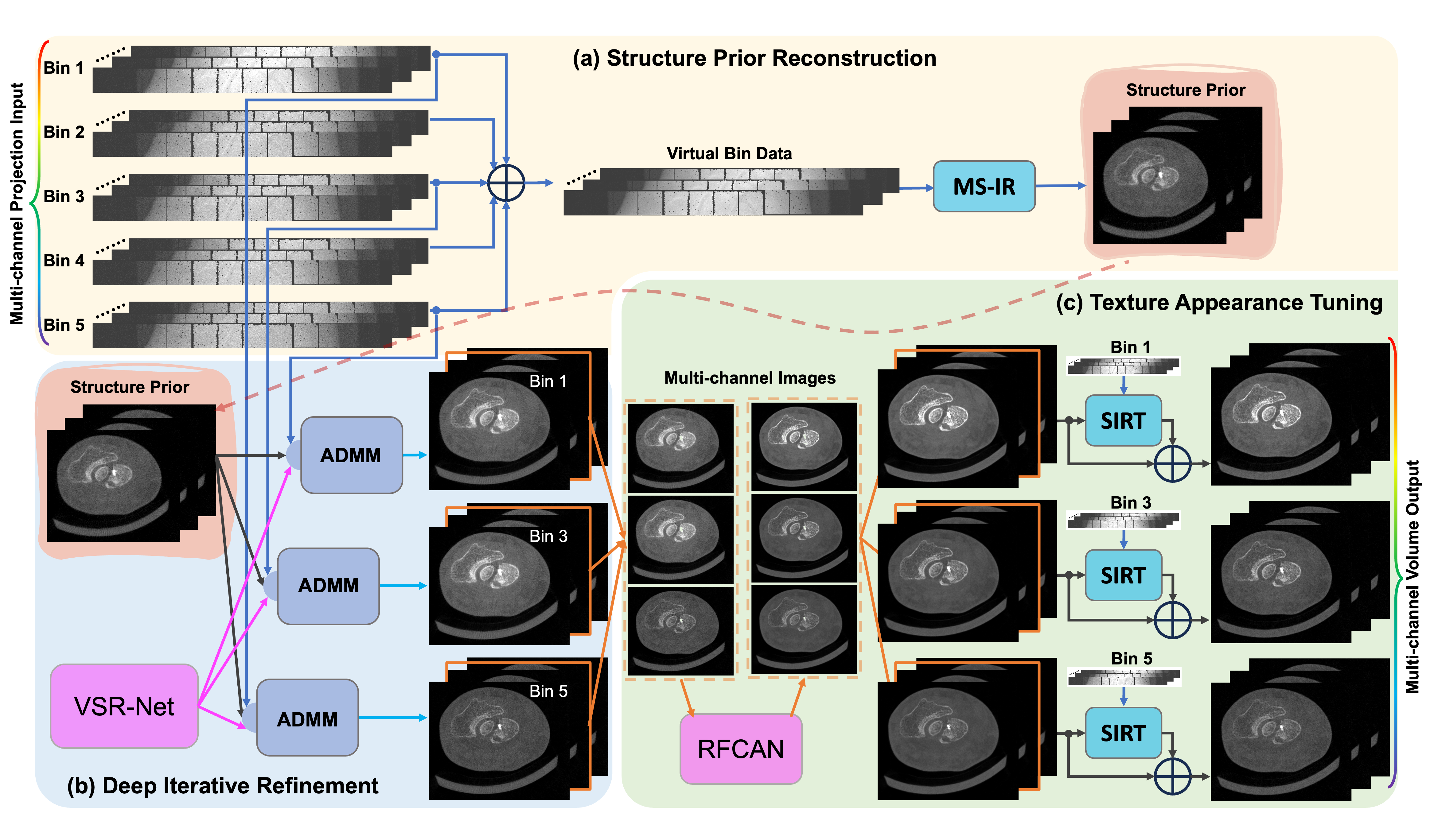
Figure 1: Overview of the deep few-view PCCT reconstruction workflow. (a) A less noisy structural prior is reconstructed from a virtual bin data, obtained by summing counts from all channels of few-view projections, with a multi-scale iterative reconstruction (MS-IR) technique. (b) For image reconstruction in each channel, the structural prior is iteratively refined with a Volumetric Sparse Representation Network (VSR-Net) and model-based guidance from the projection measurements in an Alternating Direction Method of Multipliers (ADMM) optimization framework. The network is trained with synthetic data and special techniques are used to address the domain gap issues. (c) The texture and appearance of the multi-channel images are further touched with a Residual Fourier Channel Attention Network (RFCAN) for feature enhancement and value alignment with MARS proprietary reconstructions, and followed by mixing with the result of further iterations with Simultaneous Iterative Reconstruction Technique (SIRT) for image sharpness and noise characteristics preferred by radiologists.

II-A MARS Extremity PCCT

The clinical trail was performed on the state-of-the-art MARS Extremity 5X120 scanner, which can simultaneously measure up to eight energy windows/bins at spatial resolution $50\mu m$-$200\mu m$. It enables identification and quantification of various components of soft tissues, bones, cartilage, and exogenously administered contrast agents and pharmaceuticals in a single scan. The system includes CdZnTe/CdTe-Medipix3RX detectors with $110\mu m$ pixel pitch, a $350\mu A$ X-ray source (up to $120kVp$), a rotating gantry for helical scanning, and a visualization workstation and MARS software for spectral and material analysis. It provides $90\mu m$ voxel size with reduced metal artefacts for evaluation of bone surrounding metalware. The bore size is $125mm$ for scanning extremities with a scanning length of $35cm$. Compared to conventional CT systems, it has lower radiation dose with improved image quality and material discrimination.

II-B Reconstruction with Structural Prior

Each element of the MARS PCD counts with 5 effective energy thresholds simultaneously, resulting in quasi-monochromatic projections in 5 energy bins: i.e., $7-40keV$, $40-50keV$, $50-60keV$, $60-70keV$, and $70keV$ above. Patient scans are performed in low dose mode, and the recorded count of total incoming photons is around 1,500 per detector element for open beam measurements, resulting in only hundreds of photons in one channel. Given such low counts, direct reconstruction from the photons in each energy bin inevitably suffers from major quantum noise. Instead, we notice that the structural information between different energy bins are closely correlated with only slight attenuation value difference. Based on this fact, we propose the following steps to obtain the spectral reconstructions in 5 energy bins with minimized quantum noise: (1) We sum the counts from all channels to form a virtual ‘integrating’ bin with minimized quantum uncertainty; (2) We reconstruct from the virtual bin to obtain an image with minimized noise and use it as the structural prior for all other bins; (3) Leveraging the inter-bin similarity, we initialize our iterative deep reconstruction method with the structural prior, and feed in the real bin data to reconstruct the spectral image in each energy bin.

In this way, the compromised structural information in one energy bin can be effectively recovered from data in other bins. The correct attenuation information is restored from bin-specific measurements, under the image sparsity constraint on the manifold defined by the deep learning prior. A multi-scale iterative reconstruction strategy is used to significantly accelerate the convergence for the large volume reconstruction.

II-C Deep Iterative Refinement (DIR)

To address the challenge of lacking proper training data, we propose to use synthetic data for network training and use several strategies to minimize the effects of domain gap issues. First, we limit the function of network to low-level feature denoising which is more robust to domain gaps compared to generative tasks of high-level structure synthesis due to the low-level structural similarities in images. Second, a patch-based training strategy is employed to help minimize domain gap leveraging the low-level similarity. Last, we use model-based iterative refinement to further correct the gap errors in the loop, guided by physical knowledge. The patch-based volumetric denoising and model-based iterative refinement are integrated in the optimization framework of alternating direction method of multipliers .

II-C1 Alternating Direction Method of Multipliers (ADMM) Optimization

The solution space under data constraint is often high-dimensional for a few-view or low-dose CT reconstruction problem. Although the true solution is unique, many images containing artifacts could satisfy the data constraint, requiring us to incorporate prior knowledge to select a desirable image that is the closest to the truth. Mathematically, this is formulated as an optimization problem:

$$\bm{x}^{*}=\operatorname*{arg\,min}_{\bm{x}}\frac{1}{2}{\left\lVert A\bm{x}-\bm{y}\right\rVert^{2}+\lambda R(\bm{x})},$$ (1)

where $A\in\mathbb{R}^{M\times N}$ and $\bm{y}\in\mathbb{R}^{M}$ are a system matrix and a projection vector respectively, $\bm{x}\in\mathbb{R}^{N}$ denotes an image volume to be reconstructed, and $R(\cdot)$ is the regularization term to incorporate the prior knowledge.

To solve Eq. (1) with deep prior, an auxiliary variable $\bm{z}$ is introduced to decouple the prior term from the loss function as follows:

$$\bm{x}^{*}=\operatorname*{arg\,min}_{\bm{x}}\frac{1}{2}{\left\lVert A\bm{x}-\bm{y}\right\rVert^{2}+\lambda R(\bm{z})},\quad\text{s.t.}\quad\bm{z}=\bm{x}.$$ (2)

The augmented Lagrangian of Eq. (2) is [28]

$$\mathcal{L}_{\mu}(\bm{x},\bm{z},\bm{v})=\frac{1}{2}\left\lVert A\bm{x}-\bm{y}\right\rVert^{2}+\lambda R(\bm{z})+\bm{v}^{T}(\bm{x}-\bm{z})+\frac{\mu}{2}\left\lVert\bm{x}-\bm{z}\right\rVert^{2},$$ (3)

which becomes a saddle point problem and can be solved using the alternating direction method of multipliers (ADMM) [29, 30] as follows:

$$\left\{\begin{array}[]{l}\bm{x}^{k+1}=\operatorname*{arg\,min}_{\bm{x}}\frac{1}{2}\left\lVert A\bm{x}-\bm{y}\right\rVert^{2}+\frac{\mu}{2}\left\lVert\bm{x}-\bm{z}^{k}+\frac{\bm{v}^{k}}{\mu}\right\rVert^{2}\\ \bm{z}^{k+1}=\operatorname*{arg\,min}_{\bm{z}}\lambda R(\bm{z})+\frac{\mu}{2}\left\lVert\bm{x}^{k+1}-\bm{z}+\frac{\bm{v}^{k}}{\mu}\right\rVert^{2}\\ \bm{v}^{k+1}=\bm{v}^{k}+\mu(\bm{x}^{k+1}-\bm{z}^{k+1})\\ \end{array}\right.$$ (4)

where $\mu$ is a hyper-parameter and $\bm{v}$ is the augmented Lagrange multiplier.

As formulated in Eq. (4), the overall optimization problem is decomposed into sub-problems that are easier to solve and can be successively optimized to obtain the final solution. Clearly, other constraints or priors can be included in this framework.

It is worth mentioning that for each sub-problem it is not necessary to find the minimizer exactly in a single iteration. Instead, decreasing the loss incrementally is enough, which is often helpful for computational acceleration [29].

The optimization of $\bm{x}$ can be achieved by using the gradient descent method for a number of steps with a step size $\beta$:

$$\nabla\mathcal{L}_{\mu}(\bm{x}) =A^{T}(A\bm{x}-\bm{y})+\mu(\bm{x}-\bm{z}^{k}+\bm{v}^{k}/\mu),$$ (5)

$$\bm{x}^{k,(t+1)} =\bm{x}^{k,(t)}-\beta\nabla\mathcal{L}_{\mu}(\bm{x}^{k,(t)}).$$

where $(t)$ represents the step number of gradient descent method. The optimization of $\bm{z}$ is actually a proximal operation:

$$\bm{z}^{k+1}=\text{prox}_{\frac{\lambda}{\mu}R}(\bm{x}^{k+1}+\bm{v}^{k}/\mu).$$ (6)

As shown in a previous analysis, the learned denoiser resembles a projection of the noisy input onto a clean image manifold [31], and this claim is supported by several recent applications using deep networks as learned proximal operators [32, 33]. Following the same idea, here we use our network to approximate the proximal operation as a deep prior.

Note that the noise characteristics (type, distribution, and parameters) could change through iterations. Especially, the noise at earlier stages may majorly differ from that at later stages. However, the network denoiser is often trained for mapping a final noisy CT reconstruction to its corresponding clean label. To reduce the domain gap of noise and accelerate the reconstruction, we initialize $\bm{x}$ with the results obtained with the structural prior. Meanwhile, the magnitude of noise in the reconstruction gradually diminishes to a small level as the number of iterations grows large. Hence, we could reduce the network contribution at later stages since the network is often not trained to have a fixed point. As a result, Eq. (6) is reformulated with a network denoiser as follows:

$$\bm{z}^{k+1}=\gamma f_{\theta}(\bm{x}^{k+1}+\bm{v}^{k}/\mu)+(1-\gamma)(\bm{x}^{k+1}+\bm{v}^{k}/\mu),$$ (7)

where $\gamma$ controls the network contribution, which can be understood as a parameter to control the amount of noise to be removed during the iterative process.

II-C2 Volumetric Sparse Representation Network (VSR-Net)

Despite the great success achieved with many deep reconstruction methods for 2D CT images, directly applying them to clinical HR PCCT imaging is almost infeasible with the conventional GPUs. The GPU memory cost for image volume, sinogram storage, and the corresponding backward/forward projection operations becomes a very challenging problem for HR volumetric imaging, invalidating direct methods like AUTOMAP [34] and many other unrolling methods [14, 35]. Rather than training a network that learns a global representation of a whole volume, we train a network that learns a patch-based representation to overcome the memory limit for volumetric image reconstruction. The architecture of our proposed network is illustrated in Fig. 2. It is a light-weight 3D network that combines U-Net [36] and ResNet [37] structures with 3D grouped convolutions  [38] and special 3D pixel shuffle operations to promote application speed and performance.

In contrast to many generative networks using large reception fields for realistic high-level feature synthesis, we intentionally force the network to concentrate on low-level features by choosing a small kernel size of $3\times 3\times 3$ for all convolution layers, hoping to gain more tolerance to domain gaps by leveraging low-level structural similarities between images from different applications. Compared to widely used 2D convolution, we use a 3D grouped convolution for all convolution layers to fully utilize the information from neighboring voxels. To facilitate training and boost performance, the grouped convolution is used to enforce structural sparsity, encouraging the differentiation between feature maps, and to construct a bigger network with less trainable parameters. Different from conventional downscale/upscale operation using convolutions with strides, we used 3D pixel unshuffle/shuffle operation for this purpose as shown in Fig. 2(b). The unshuffle operation splits the input volume into 8 sub-volumes and concatenates them in the channel dimension, while the shuffle operation assembles the sub-volumes into a super volume. The benefits of such operations are as follows: with unshuffle, we can explicitly generate multiple repetitive LR measurements from the HR volume to extract signals from the noisy background with the subsequent convolution layers; then, the shuffle operation assembles the denoised LR sub-volumes into a resolution-enhanced version. Per the suggestion in [39], we omit batch normalization throughout the network, and the first and the last convolution layers involve no activation. To maintain the scaling invariance and promote the network generalizability, no bias is used in all layers as suggested in [33]. The cube size for network training can be adjusted according to the available GPU memory. We set the cube size to 32 in our experiments, and the network can be easily deployed on a conventional commercial 1080Ti GPU with 11GB memory.

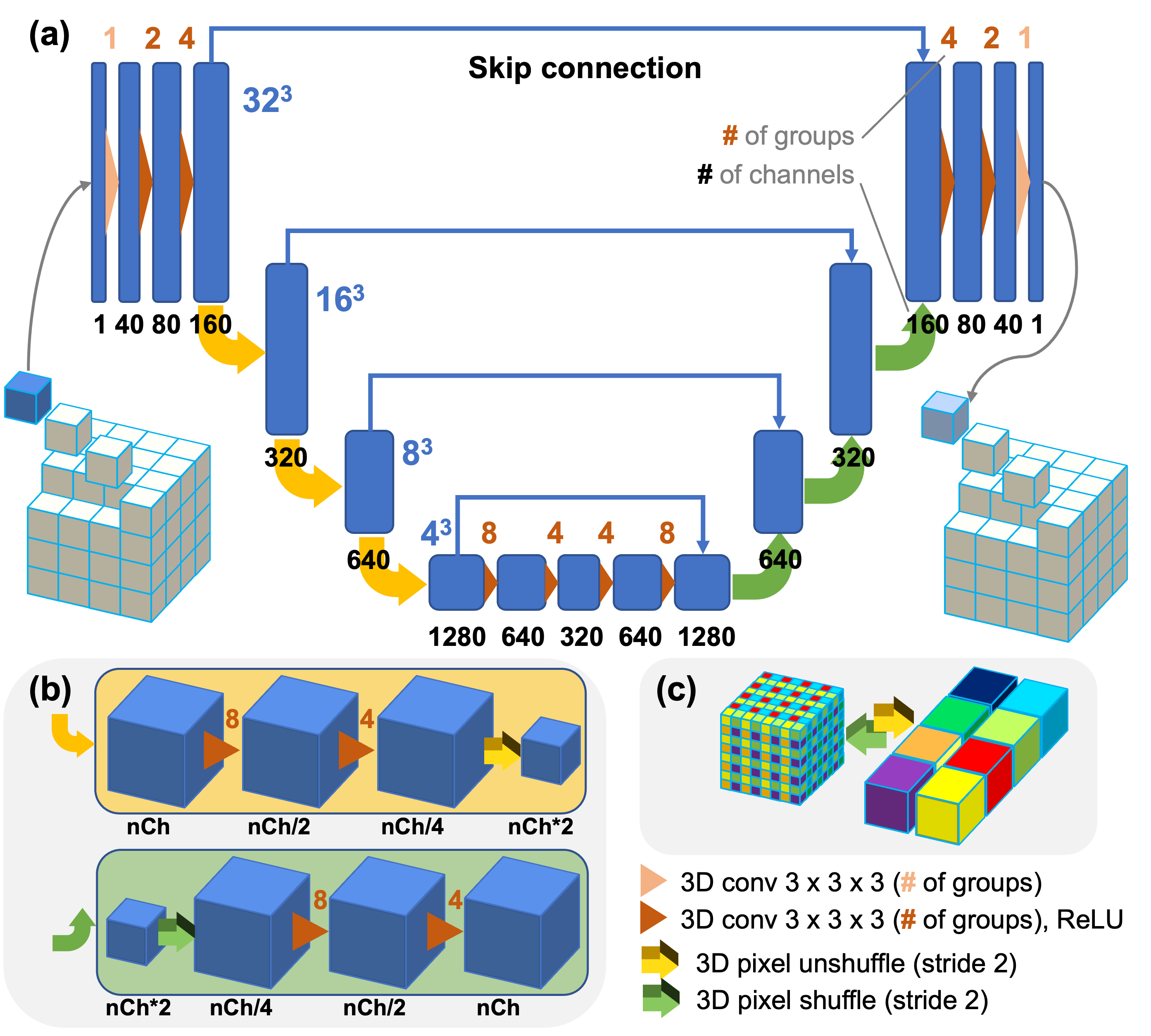
Figure 2: Architecture of our volumetric sparse representation network (VSR-Net). (a) This light weight network takes a small cubic patch as input and outputs a denoised patch. 3D pixel shuffle operations and grouped convolutions are used to promote speed and performance; and (b) The downscaling and upscaling of feature maps are achieved through 3D pixel unshuffle and shuffle operations (illustrated in (c)) combined with two 3D grouped convolutional layers. Note that Conv, grouped convolutional layer; ReLU, rectified linear unit; a color-coded number above each convolutional operation denotes the number of groups used, while the number underneath the feature map indicates the number of channels.

II-C3 VSR-Net Training with Synthetic Data

Since it is rather challenging to obtain the ground truths for HR patient scans, we use synthesized data for network training. Specifically, we construct our training dataset from the open dataset for the Low-dose CT Grand Challenge [40]. We first resize the images to have isotropic voxels of $1mm$ along each dimension, and convert the voxel values in the Hounsfield unit to the linear attenuation coefficients. Then we treat volumes as digital phantoms of $0.2mm$ voxel size and generate noise-free projections using a MARS CT scanner geometry despite with a flat PCD and in circular cone beam mode. Finally, the projections with quantum noise are simulated assuming 16,000 incident photons per detector element. The Simultaneous Iterative Reconstruction Technique (SIRT) is used to reconstruct images.

The isotropic volumes and corresponding noisy reconstructions are the labels and noisy inputs for network training. Ten patient volumes are partitioned into cubes of size $32^{3}$ with a stride of 25 pixels along each direction. Then, the cubes are sieved to remove empty ones based on the standard deviation of pixel values. As a result, over 190,000 pairs of 3D patches are generated for training, and around 38,000 pairs for validation. The loss function consists of a $L_{1}$ norm term for the value difference and a mean square error term for the relative value difference:

$$\sum_{i}\left[\left\lVert\bm{y}_{i}-f_{VSR}(\bm{x}_{i};\theta)\right\rVert_{1}+\beta_{0}\left\lVert\frac{\bm{y}_{i}-f_{VSR}(\bm{x}_{i};\theta)}{\bm{y}_{i}+c}\right\rVert^{2}_{2}\right],$$ (8)

where $\bm{y}_{i}$ and $\bm{x}_{i}$ are respectively the label patches and noisy inputs, $f_{VSR}(\bm{x}_{i};\theta)$ corresponds the network output with trainable parameters $\theta$, and $c$ is a constant to avoid zero denominator. The $L_{1}$ norm, instead of the $L_{2}$ norm, is used in the first term to avoid blurring details, and the relative error is measured with the $L_{2}$ norm in the second term to preserve tiny structures based on our experience [41]. During training, we set the balancing hyperparameter $\beta_{0}$ to 1 and $c$ to 0.1.

II-C4 Parallel Batch Processing & Geometric Self-ensemble

During the inference, reconstruction volume is partitioned into overlapping patches then fed into the VSR-Net. Geometric self-ensemble based on flipping and rotation is also adapted to boost performance and suppress check-board artifacts. To save computation, we randomly choose 1 of 8 transforms to apply on the reconstruction volume for each iteration which is similar to periodical geometric self-ensemble idea [33]. For acceleration, parallel processing technique has been used to distribute the workload onto multiple GPUs to deal with the huge amount of patches.

II-D Texture Appearance Tuning

We leverage the structural prior to reduce noise and accelerate convergence, and use a channel-by-channel reconstruction strategy for deep iterative refinement to reduce the memory burden for single node reconstruction and allow parallel reconstruction with multiple nodes. To match image spectral values with those from proprietary reconstruction that radiologists are familiar with, we adopt a two-step procedure to fine tune the texture and appearance. First, we use a 2D convolutional network to exploit the inter-channel correlation for texture enhancement and value alignment. Multi-channel images extracted from the channel reconstructions at the same slice are fed to network for the mapping, in a slice-by-slice manner for memory efficiency and performance. Then, we further process the reconstruction with SIRT for a few iterations to enhance image sharpness and alter noise characteristic. By mixing the network processed results before and after SIRT iterations at a preferred ratio based on radiologists’ feedback, the final output with consistent appearance with MARS reconstruction is obtained.

II-D1 Residual Fourier Channel Attention Network (RFCAN)

We make our value alignment network by modifying the residual channel attention network [42] to adopt a more advanced Fourier channel attention mechanism [43] and learn a multi-channel mapping between the input and output, as illustrated in Fig. 3. For the training of RFCAN, we use the full-view MARS reconstruction slices as the label for our half-view reconstruction results. However, due to patient motions and the black box nature of propriety reconstructions, there can be occasional non-rigid misalignment across a few slices between our reconstruction and the MARS results, resulting from differences in volume splitting and projection partitioning during HR reconstruction, and number of projections. Hence, we select one patient scan that is least affected by motions as our training data, and then sieve out the misalignment-affected slices, resulting 584 pairs of HR multi-channel images ($1200\times 1200$). A total of 206,000 pairs of overlapping patches of size $128\times 128$ are randomly extracted from the images for network training, and around 52,000 pairs for validation. Additional penalty on the Fourier spectrum is introduced in the loss function to emphasize the texture similarity besides the spatial intensity fidelity imposed by other terms:

$$\sum_{i}\Bigl{[}\left\lVert\bm{y}_{i}-f(\bm{x}_{i};\theta)\right\rVert_{1}+\beta_{1}\left\lVert\frac{\bm{y}_{i}-f(\bm{x}_{i};\theta)}{\bm{y}_{i}+c}\right\rVert^{2}_{2}$$

$$+\beta_{2}\left\lVert\mathcal{FFT}(\bm{y}_{i})-\mathcal{FFT}(f(\bm{x}_{i};\theta))\right\rVert_{1}\Bigr{]},$$ (9)

where $\mathcal{FFT}(\cdot)$ denotes the Fourier transform. $\bm{y}_{i}$, $\bm{x}_{i}$, and $f(\bm{x}_{i};\theta)$ are the label, input, and network output, respectively. The balancing hyperparameters $\beta_{1}$ and $\beta_{2}$ are both set to 1 with $c$ set to 0.1 during training.

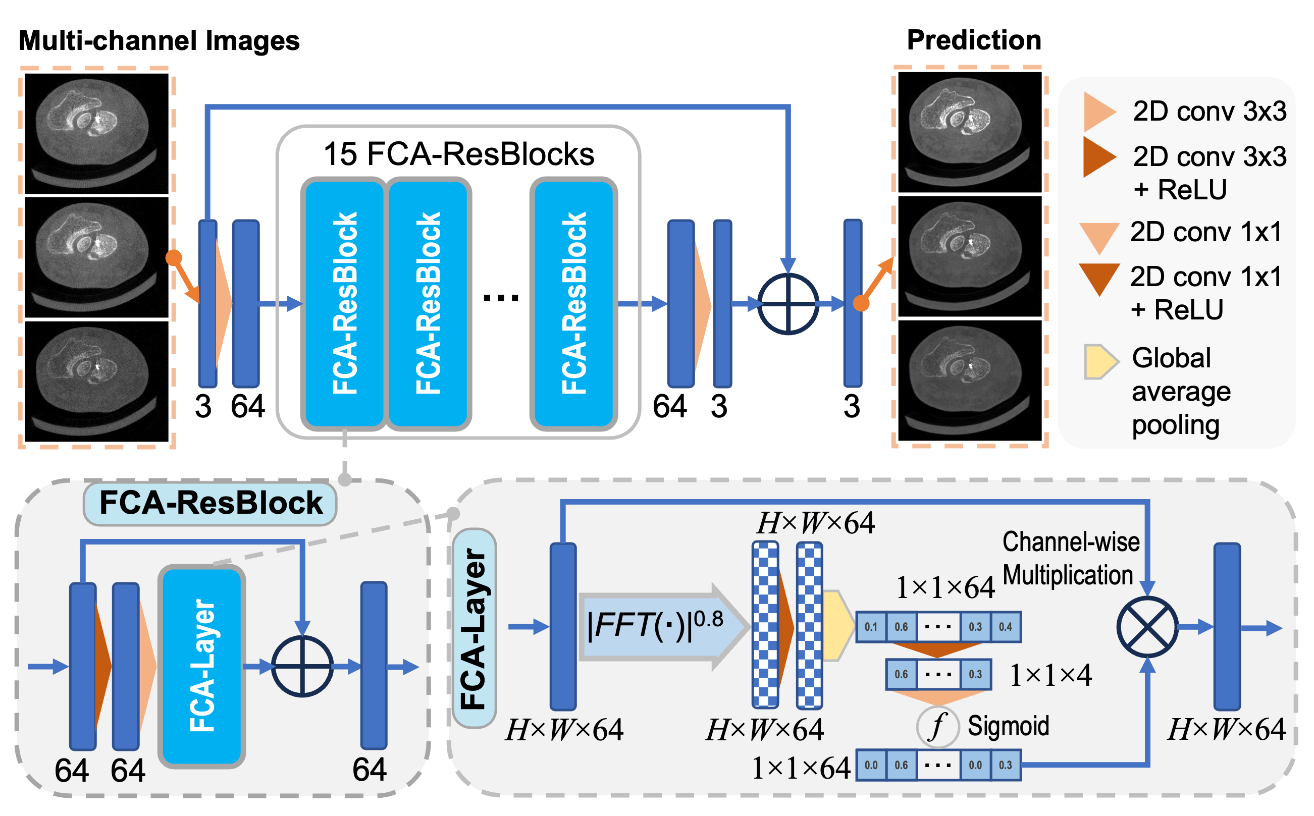
Figure 3: Architecture of the residual Fourier channel attention network (RFCAN), consisting of 15 Fourier channel attention residual blocks (FCA-ResBlocks) built upon attention layers with FCA (FCA-Layer).

II-E Interleaved Updating for Large Volume Reconstruction

The size of projection data from a patient scan can be huge, e.g., $1536\text{~{}columns}\times 128\text{~{}rows}\times 3392\text{~{}views}\times 5\text{~{}channels}$., overwhelming the GPU memory for direct reconstruction. Besides the channel-by-channel reconstruction technique described earlier, to alleviate memory burden we further use a interleaved updating technique to divide large volume reconstruction job into a batch of mini-jobs of smaller size by partitioning the projection data and reconstruction volume into different segments as illustrated in Fig. 4. The volume as well as the projection data is partitioned into $N$ segments, and each volume segment and corresponding projection data segment are carefully aligned in geometry. To ensure the data completeness everywhere, sub-volumes at the seams are also extracted with their corresponding projection data (about 1.5 to 2 rotations from the helical scan). The volume segments and seams form $2*N-1$ mini-reconstruction tasks, which are assigned to multiple GPUs for parallel computing with multi-threads or can be processed sequentially with a single GPU if on a budget server. The resultant sub-volumes are combined together in an interleaved pattern, with a few slices at one or both ends trimmed off to ensure data completeness of the resting volume and avoid overlapping, forming a complete large volume reconstruction update as shown in Fig. 4 (b).

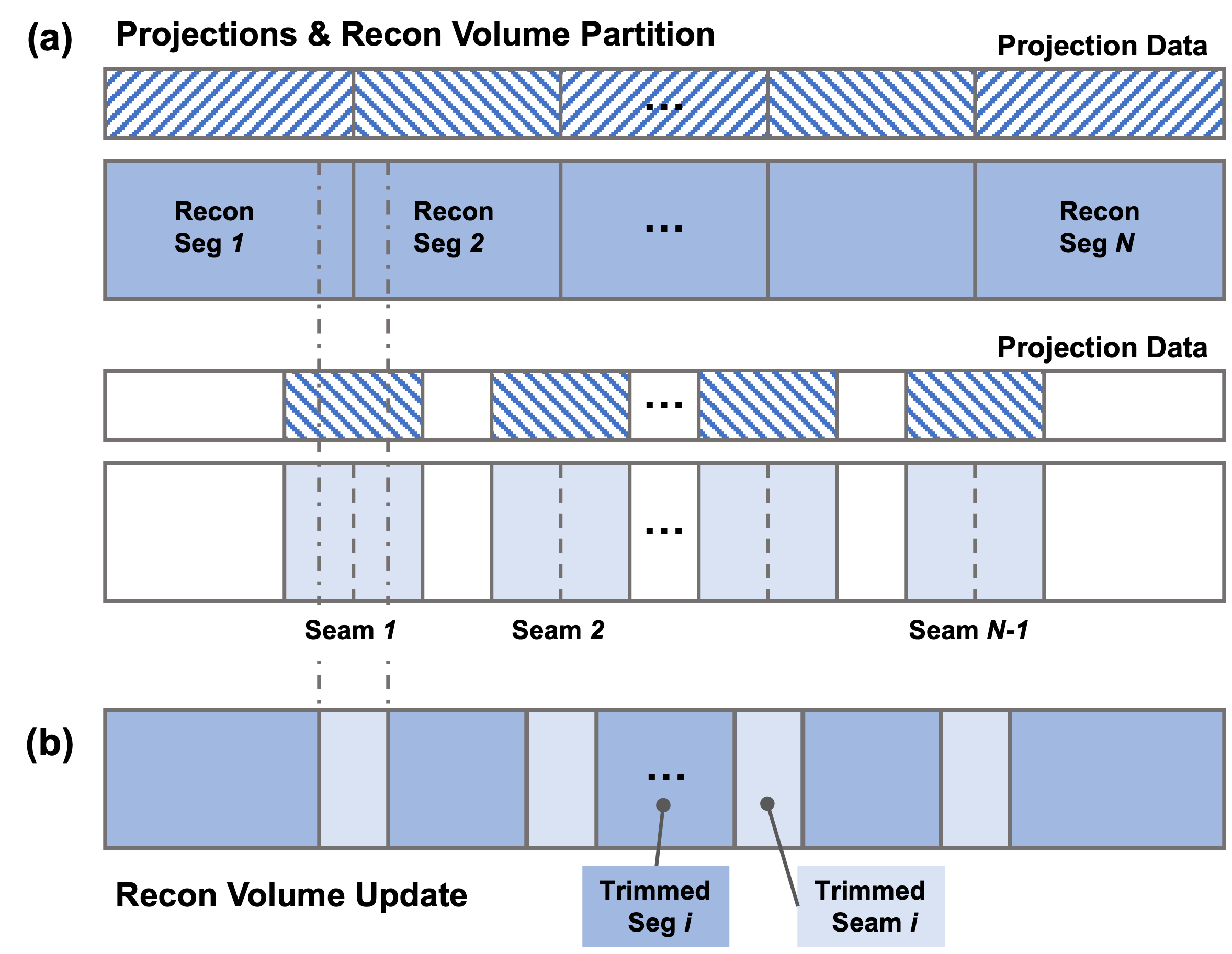
Figure 4: Interleaved updating for large volume reconstruction: (a) partitioning the projections and reconstruction volume to form a batch of reconstruction tasks on sub-volumes; and (b) combining the results in an interleaved pattern with slices at one or both ends trimmed off to ensure data completeness and avoid overlapping.

III Experiments and Results

III-A Implementation and Experimental Setup

Training Details. Our VSR-Net and FRCAN are implemented on PyTorch and trained with Adam optimizer on a single NVIDIA V100 GPU. The learning rate for VSR-Net is initially $2\times 10^{-4}$ and decayed by 0.95 every epoch. The total number of epochs is 60 with a batch size of 32. The learning rate for FRCAN is initially $1\times 10^{-4}$ and decayed by 0.6 every epoch, with a total of 10 epochs and a batch size of 32. The VSR-Net is trained on synthetic dataset described in Sec. II-C3, while FRCAN is trained on real patient data as described in Sec. II-D1.

Reconstruction Details. We use the ASTRA Toolbox [44] for GPU-based forward and backword projection operations. The patient data are reconstructed on a cluster node with eight NVIDIA V100 GPUs for parallel computation (parallel sub-volume reconstruction and patch processing), and other data are reconstructed on a server with a single RTX A5000 GPU.

Experimental Setup. First, we demonstrate the in-domain capability of our DIR method on synthetic single channel CT data. The testing volume is generated from AAPM dataset following a similar simulation protocol but from non-overlapping patients. Then, we demonstrate the enhanced generalization on out-of-domain data with our DIR compared to the conventional post-processing way of applying VSR-Net. We use phantom data, with disparate structures from training data, scanned from a micro-PCCT system for out-of-domain testing. Finally, we validate our whole PCCT reconstruction workflow (DIR followed by texture appearance tuning) on real patient data acquired on the MARS Extremity scanner. Ratings from radiologists on diagnostic value are used to assess the effectiveness of our method.

III-B In-domain Simulation Study

We first evaluate our deep iterative refinement method on simulated in-domain cone-beam CT data. Specifically, a numerical flat panel detector consists of $1536\times 128$ pixels of $0.11mm$ pitch. The source-to-detector distance and the source-to-isocenter distance are $949mm$ and $625mm$, respectively. Over a full scan, 373 projections are evenly collected, and the number of incident photons per detector element is set to 16,000 in an empty scan. The reconstruction volume is set to $420\times 420\times 60$ of $0.2^{3}mm^{3}$ voxels. The SIRT reconstruction from clean projection data with 500 iterations serves as the ground truth. The standard FDK (ramp filter) reconstruction from noisy projection data reveals the severity of image noise. It is underlined that most existing CT image deep denoising methods are based on post-processing FBP/FDK reconstructions, and will not deliver the optimal imaging performance.

Our proposed method is compared against the anisotropic total variation (TV) [45] regularized SIRT reconstruction (SIRT-TV) in both full-view and half-view scenarios [46]. SIRT-TV is a representative compressed sensing method to minimize the cost function in the following form:

$$\bm{x}^{*}=\operatorname*{arg\,min}_{\bm{x}}{\frac{1}{2}\left\lVert A\bm{x}-\bm{y}\right\rVert^{2}+\lambda TV(\bm{x})}.$$ (10)

The proximal gradient descent method is used to solve the problem, and $\lambda$ is an empirical parameter. The regularization parameter $\lambda$ for SIRT-TV is respectively set as $9.0\times 10^{-4}$ and $1.5\times 10^{-4}$ for full-view and half-view reconstructions for their best results. In our method applying DIR to half-finished SIRT reconstruction, the settings $\mu=0.01,\beta=0.5,\gamma=0.8$ and $\mu=0.015,\beta=0.5,\gamma=0.8$ are used for full-view and half-view cases respectively, and the number of gradient descent steps per iteration was set to 10 in both cases.

Representative full-view and half-view reconstructions are shown in Fig. 5. The fine details indicated by the red arrows are successfully restored with our methods for both full-view and half-view cases while missing structures or distortions are observed with the SIRT-TV particularly in the half-view scenario. Additionally, unnatural waxiness is also observed in the zoom-in regions of SIRT-TV results. Moreover, our half-view reconstruction scores are even better than the full-view reconstruction with the conventional method in terms of structural similarity index metric (SSIM) and peak signal-to-noise ratio (PSNR) metric, demonstrating the superiority of our method. More importantly, our method demonstrates impressive stable performance despite significant acquisition condition change from full-view to half-view ($<1.0\%$ loss in SSIM and $<4.0\%$ loss in PSNR), which is even more robust than the classic SIRT-TV.

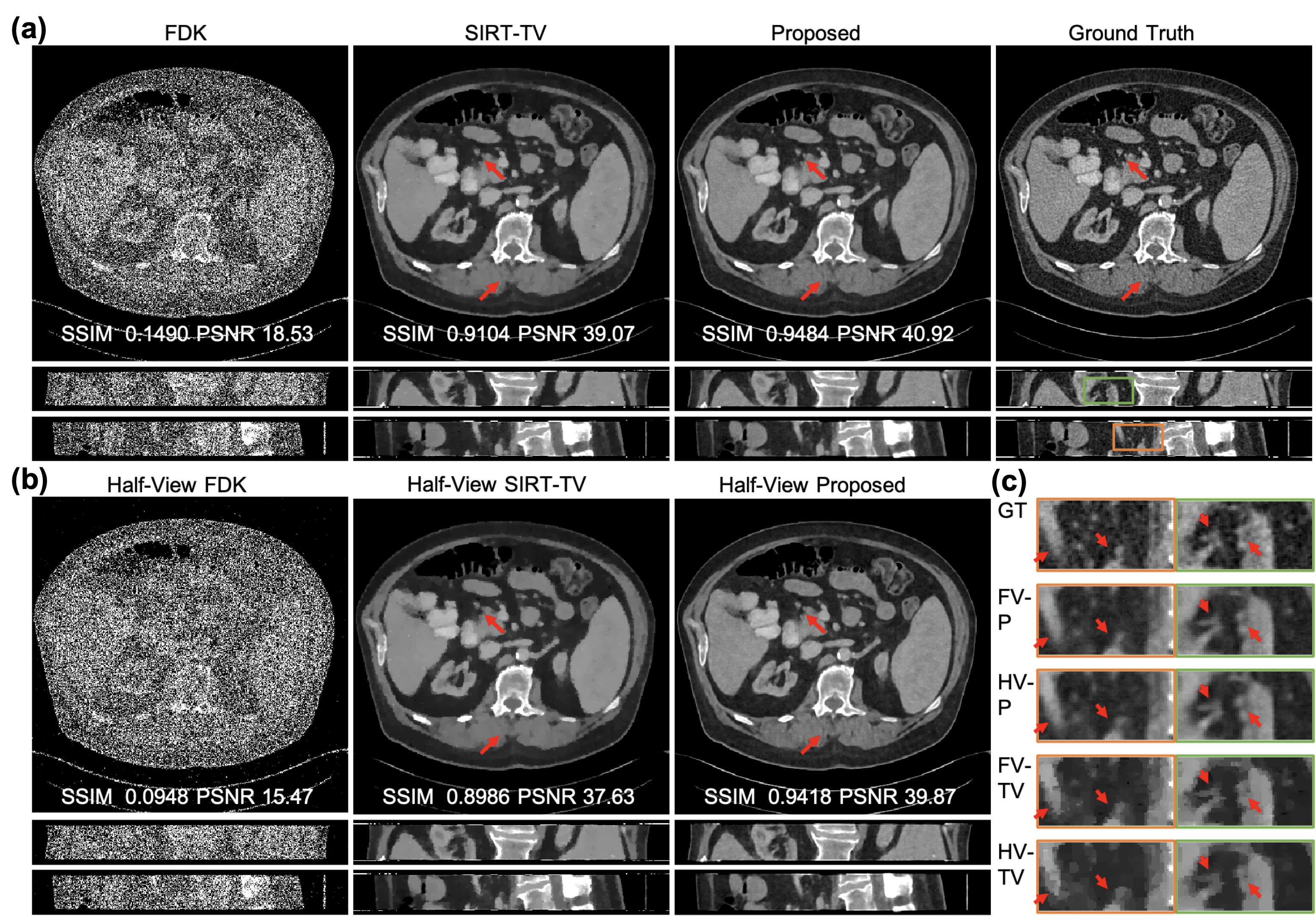
Figure 5: Representative images reconstructed using competing methods on simulated data. (a) The full-view reconstructions with FDK, SIRT-TV, and our method displayed against the ground truth, with exemplary axial, coronal, and sagittal views included from top to bottom; (b) the reconstructions from halved views; and (c) magnified regions from the coronal and sagittal views as indicated by the green and orange boxes respectively and displayed in the descent order of image sharpness and structural fidelity: ground truth (GT), our full-view and half-view reconstructions (FV-P, HV-P), and full-view and half-view reconstructions with SIRT-TV (FV-TV, HV-TV) from top to bottom. The display window is W/L:400/50 HU. The red arrows indicate the structural details are easy to recover for our methods but challenging for SIRT-TV.

III-C Out-of-domain Phantom Studies

To demonstrate the enhanced generalizability on out-of-domain data, we further test our DIR method on phantom data with totally different structures as shown in Fig. 6. The single-channel helical scan data were acquired on our custom-built micro-CT system equipped with a PCD (ADVACAM WidePIX1x5, Prague, Czech Republic) at 80$kVp$. We collected the data at five different dose levels by adjusting the exposure time per projection (0.15, 0.5, 1.0, 1.5, 2.0, and 5.0 seconds). The volumes were reconstructed using 250 SIRT iterations at size $979\times 979\times 610$ with a $35\mu m$ voxel size, serving as noisy inputs and the clean reference. Post-processing with the latest BM3D [12] and with VSR-Net are the baselines for our DIR method. The standard deviation parameters for BM3D method were found by measuring the standard deviation of values in a water region after normalized with its mean. For the DIR method, we used the half-finished reconstruction as the structure prior (60 and 40 SIRT iterations at the scale of 0.637 and 1 respectively), and refined it with 36 DIR iterations (3 gradient descent steps per iteration, $\mu=0.03$, $\beta=0.5$, $\gamma=0.8$).

Figs. 6 (a) and (b) compare the results with 0.5 and 0.15 seconds exposure from the axial view and sagittal view, respectively. Fig. 6 (c) illustrates the zoomed view of a surgical tape, and (d) displays the PSNR and SSIM distributions of the axial slices and sagittal slices of the reconstructed volumes against the reference through a violin plot. Though the phantom structures and textures are different from that in training data, our method still demonstrates great performance in improving the image quality, showing good generalizability on out-of-domain structures. In contrast, the adverse effect of such a domain gap is clearly presented in VSR-Net results under low noise in Fig. 6 (c). Although the structures are enhanced with better visibility, the appearance and the intensity do not necessarily agree with the reference shown in Fig. 6 (a), e.g., the tape structure and dots pointed by the red and green arrows. Additionally, our DIR framework also improves resistance to noise in terms of structure fidelity, particularly in high-noise scenarios, as illustrated by the suppression of those abnormal white dots appeared in VSR-Net results. For example, those on the tape structure in Fig. 6 (a) and those on the background in Fig. 6 (b) are generated when the network mistakes the noise as real structures. BM3D method is structure-agnostic and intrinsically has better generalization compared to deep learning methods. These are reflected in the quantitative comparison results shown in Fig. 6 (d) where BM3D often scores the best in PSNR and SSIM metrics particularly in high-noise situations. However, although BM3D poses the best SSIM and PSNR scores, its image quality is not necessarily the best. It suffers from some resolution loss as demonstrated by the over smoothed tape structures in the zoomed region in Figs. 6 (a) and (c), and this suggests the importance of task-relevant metrics and underlines the need for radiologists’ evaluation in the medical imaging field. Please note that we aim to demonstrate the generalization improvement with DIR over VSR-Net in this experiment rather than to compete with BM3D as the phantom is intentionally selected to be distinctly different from the VSR-Net training data. Though we already achieve tied scores with BM3D in less noisy cases, superior results can be expected if we retrain the model and narrow the domain gap.

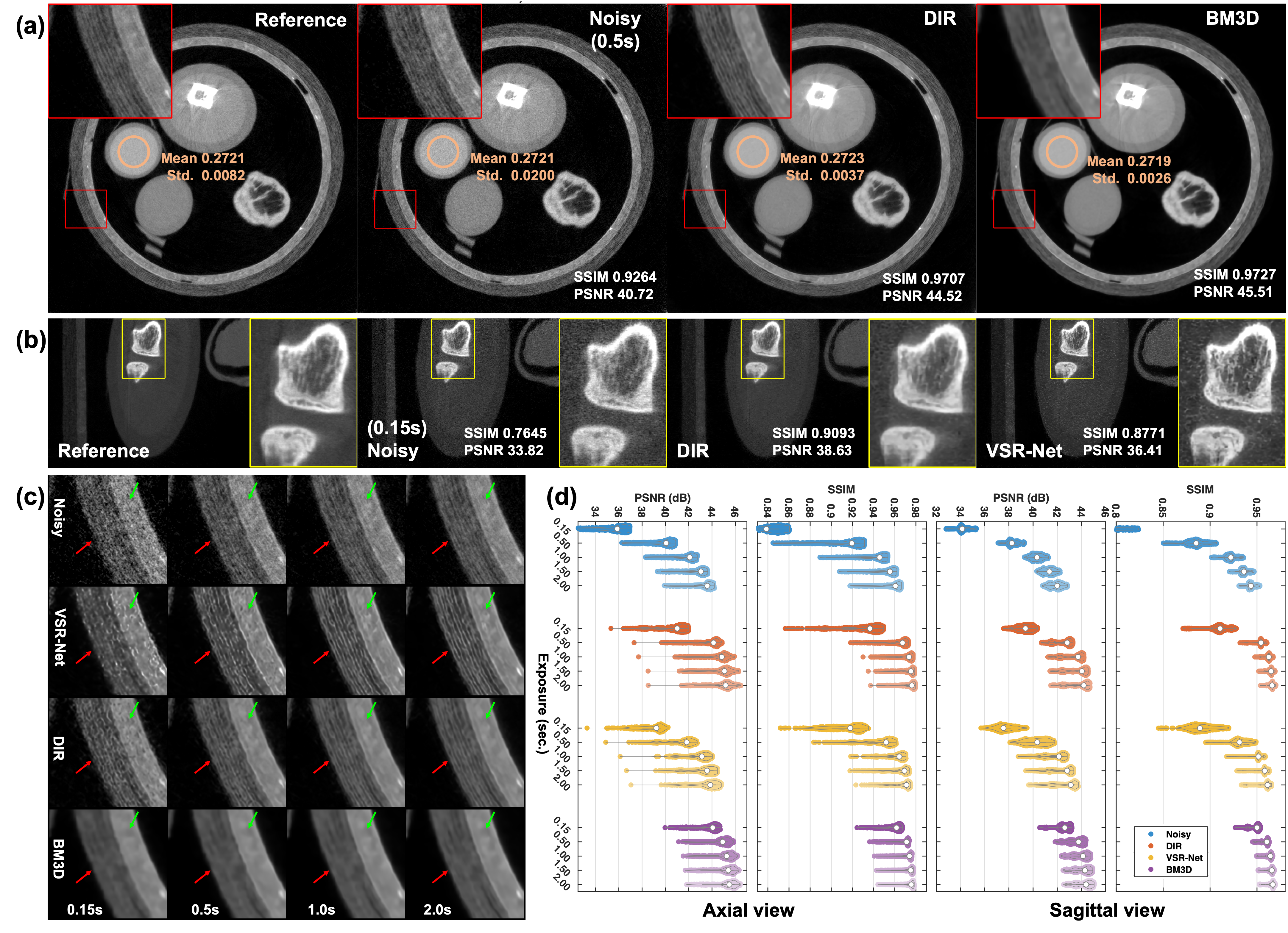
Figure 6: Out-of-domain generalization on phantom study. Comparisons between noisy input, DIR, BM3D, and VSR-Net against the long-exposure reference in: (a) axial slices from results with 0.5-second exposure; (b) sagittal slices from results with 0.15-second exposure; (c) the same magnified region as that in (a) but from results with exposures of 0.15, 0.5, 0.1, and 2.0 seconds; and (d) distributions of PSNR and SSIM values of the axial slices and sagittal slices from volumes visualized in violin plots. The display window is [0, 0.45] for axial view and [0, 1.05] for sagittal view, in unit of cm^-1. The mean and standard deviation values of a flat water region are listed for reference as well as the SSIM and PSNR values of the image.

III-D Retrospective Patient Studies

Patients aged 21 years and above referred from the fracture clinic were recruited for the clinical trial (Ethics approval:18/STH/221/AM01, Health and Disability Ethics Committee, New Zealand). The patient wrist images were acquired using our MARS Extremity PCCT scanner. The Medipix3RX PCD consists of 12 chips arranged in a non-flat arc shape. The data was acquired at $118kVp$ in a helical scan mode, using a tube current of $28\mu A$ and an exposure time of $160ms$. The images were reconstructed at $90\mu m$ using a customised polychromatic iterative reconstruction algorithm [47]. The iterative technique reconstructs a set of attenuation volumes as functions of energy from these projections, in non-overlapped energy bins. For instance, non-overlapping attenuation volumes are reconstructed in the $7-40keV$, $40-50keV$, $50-60keV$, $60-70keV$, $70-118keV$ bins, respectively.

III-D1 Experiment Setup

The images of 8 patients who provided written consents were reconstructed using the clinical proprietary algorithm from a full-view dataset and our proposed deep learning method (illustrated as Fig. 1) from a half-view dataset respectively, and then evaluated by three independent double-blinded radiologists (SG, AB, AL) on the rating scale defined in Table I based on their confidence in whether diagnostic image quality is achieved or not [48]. In our method, DIR has been applied to the structure prior (Sec. II-B, obtained with 80 and 80 SIRT iterations at the scale of 0.5 and 1 respectively) for 30 iterations (3 gradient descent steps per iteration, $\mu=0.03,\beta=0.5,\gamma=0.8$) for the reconstruction of each bin data, then the combined multi-channel volume ($1200^{3}\times 5$) are processed with RFCAN in a slice-by-slice manner for value alignment and texture enhancement (Sec. II-D), and the number of SIRT iterations is 30 and the mixing ratio is $0.5\colon 0.5$ to accommodate radiologists’ preference on image sharpness and noise characteristic.

TABLE I: Grading scale used for image quality assessment.

-2	Confident that the diagnostic criteria is not fulfilled;
-1	Somewhat confident that the criteria is not fulfilled;
0	Indecisive whether the criteria is fulfilled or not;
+1	Somewhat confident that the criteria is fulfilled;
+2	Confident that the criteria is fulfilled.

The radiologists were presented with 500 images from each patient (three energy bins $7-40keV$, $50-60keV$ and $70-118keV$) in the axial, coronal and sagittal formats. The sagittally reformatted images reconstructed using both methods and 3D rendering image using the standard method are shown in Fig. 7(a). The images were reviewed using InteleViewer (Intelerad Medical Systems). The image metrics assessed in the study were based on the “European guidelines on quality criteria for CT” for bones and joints [49]. The images were assessed on seven image quality criteria, including the visibility and sharpness of the cortical and trabecular bone, adequacy in soft tissue contrast for the visualisation of tendons, muscle and ligaments, as well as the effect of image noise (quantum noise) and artifact on the image quality.

Additionally, we also compare our result with that obtained by applying the state-of-the-art unsupervised learning method Noise2Sim [27] to the multi-channel reconstructions using 320 SIRT iterations for each channel. Despite significant enhancement over SIRT reconstruction from half-view dataset, Noise2Sim results demonstrate insufficient image quality (suffering from image blur and loss of fine structures) as shown in Fig. 7(b), hence, they are excluded from the reader study.

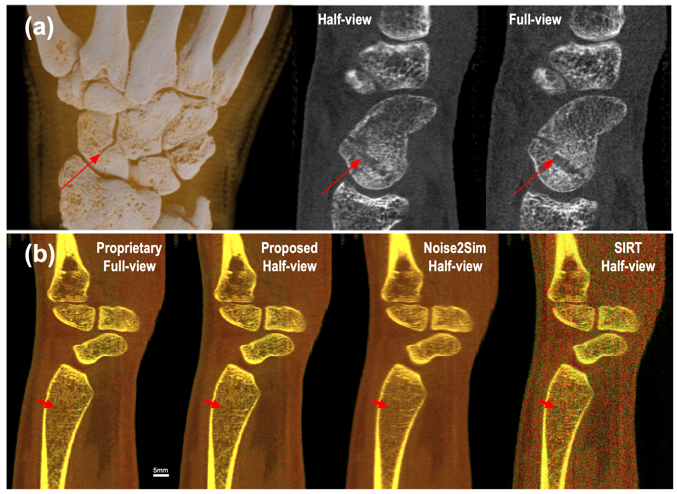
Figure 7: Sagittal reformat of a wrist joint reconstructed using standard and proposed methods respectively. (a) From left to right are 3D rendering of standard reconstruction, half-view and full-view images of channel 50-60keV. The arrow points to scaphoid fracture. (b) Color visualization of our three-channel reconstruction via linear blending [50] in reference to standard full-view result and noise2sim half-view result. Our result demonstrates high fidelity in both spectral values (same color tone and brightness as the full-view reference) and spatial structures (sharp and accurate fine details as pointed by the red arrow).

III-D2 Data Analysis

For quantitative assessment, regions of interests (ROIs), each with $\sim 250$ voxels, were drawn in the flexor carpi radialis tendon and adjacent subcutaneous fat regions in the patient images. The mean and standard deviation of linear attenuation coefficients in the ROIs were used to calculate the signal-to-noise ratio (SNR) in soft tissue regions and contrast to noise ratio (CNR) between soft tissue and fat in the ROIs. SNR and CNR values associated with both methods were compared over all patients’ datasets. For subjective evaluation, overall radiologists’ assessment grades for seven image quality measures from both methods were converted into a frequency table. Then, all three radiologists’ overall and combined ratings were compared with descriptive statistics. The hypothesis of no significant difference between the two methods was tested in the Wilcoxon signed-rank test.

Image grades from both methods in terms of each image quality measures were also converted into visual grading characteristics (VGC) points using the method described in [48]. Hence, with the current 5 images grading criteria, 4 VGC points were obtained, and 0 as the origin and 1 as the maximum value were added as well [48]. The combined VGC points (using grades from all three radiologists) of seven image quality measures were calculated, and the empirical area under the curve (AUC_VGC) were compared. The statistical significance of mean AUC_VGC of each of the seven image quality measures was analyzed through one-sample t-testing against a hypothetical AUC_VGC value of 0.5. VGC points were also obtained by combining all seven image quality measures for both methods. Full-view vs Half-view empirical AUC_VGC values and its 95% confidence intervals were obtained for each radiologist and combined scores. The statistical significance of AUC_VGC and its 95% confidence interval for each radiologist (56 samples) and all radiologists (168 samples) were interpreted according to the method described in [51]. Finally, the inter-rater agreements between radiologists were evaluated with kappa statistics. The statistical analysis was presented using GraphPad Prism 9.2.0 at a level of significance of 95%.

III-D3 Statistical Results

Image SNR in soft tissue regions and CNR between soft tissue and fat were compared in Fig. 8, where the bar charts illustrate that for all the patients, SNR and CNR in the images obtained with the proposed half-view reconstruction method are higher than that in the clinical benchmark images reconstructed using the standard proprietary method from the full dataset, except for the second one whose images showed quite comparable CNRs.

More importantly, the overall confidence ratings of diagnostic image quality with seven criteria are compared in Table II. The table shows a significantly better mean and median image quality scores with the proposed half-view reconstruction method than the current clinically used reconstruction method (proprietary reconstruction from the full-view dataset) for all radiologists despite their different scores, indicating a preference for the proposed reconstructions. The median value for the half-view reconstructions is 2 for the second radiologist, which suggests higher confidence in image interpretation. Despite the discrepancy in ratings, the combined median value is greater than 0, indicating the overall diagnostic acceptability of the images reconstructed using our method. The hypothesis was further tested in the Wilcoxon signed rank test for all three raters and combined ratings in Table III. It shows that the p-value for the Wilcoxon signed rank test is not statistically significant for the first and second radiologists, suggesting no difference in image quality from both methods. However, p-values for the other two scenarios (for the third radiologist and combined) are statistically significant, indicating the image quality from the proposed method was perceived significantly better than the proprietary method for image reconstruction from the full dataset.

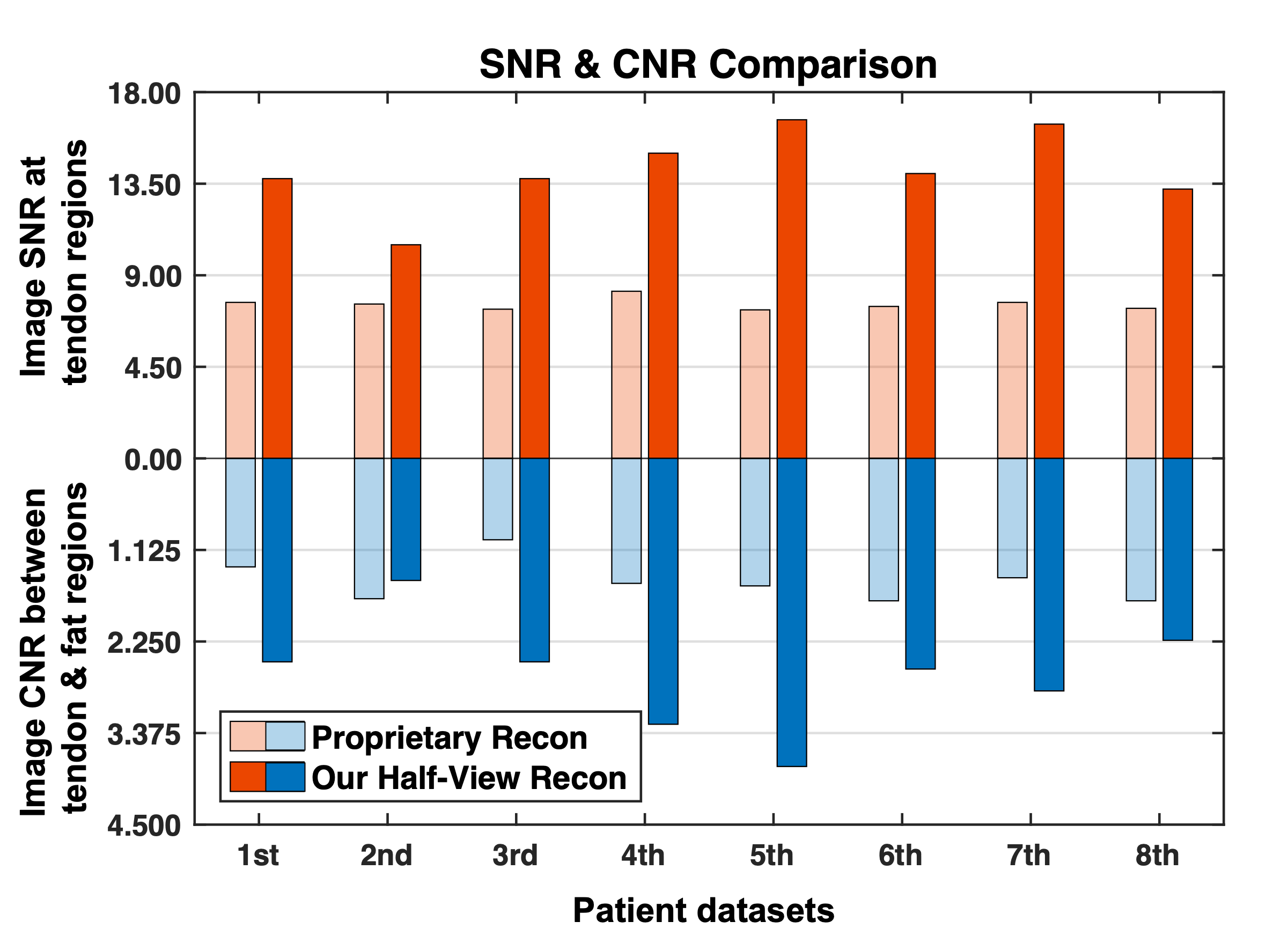
Figure 8: Quantitative evaluation of image quality of our half-view reconstruction against proprietary reconstruction from the full-view dataset.

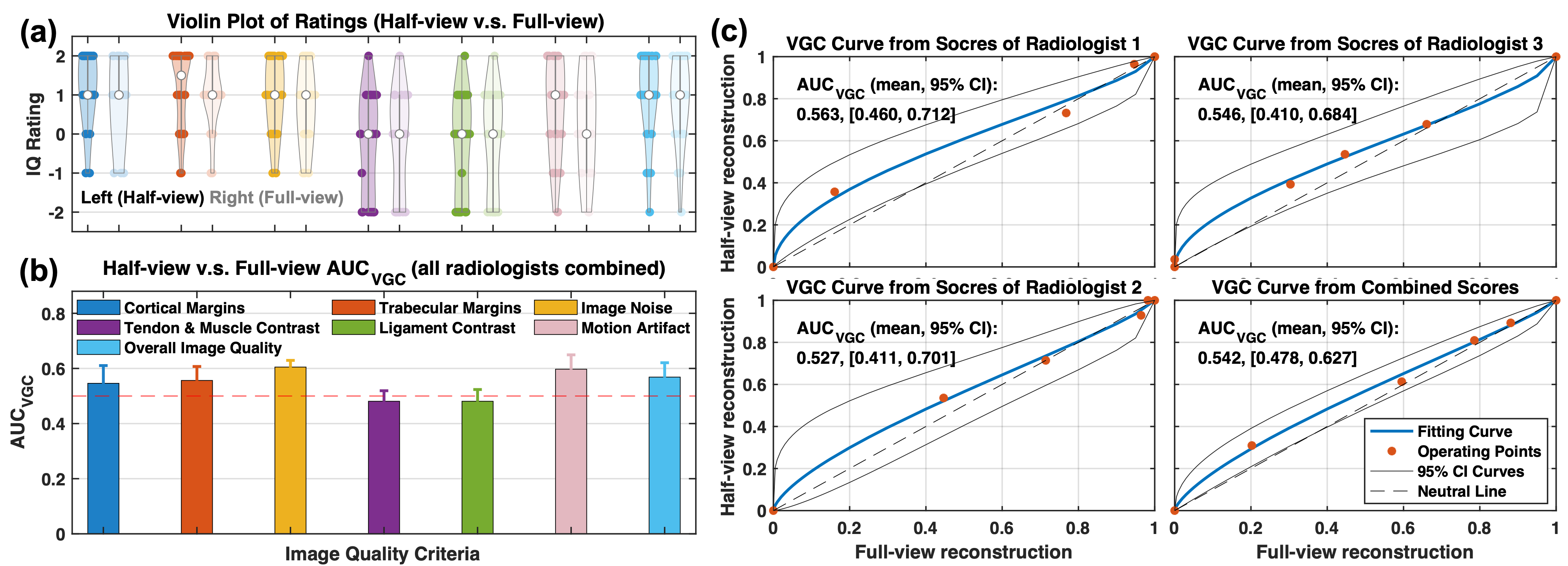
Figure 9: Subjective evaluation on seven image quality (IQ) criteria comparing our proposed half-view reconstruction and clinical full-view reconstruction. (a) Violin plot of combined radiologists’ ratings on half-view results against full-view results; (b) Slightly better than 0.5 AUC_VGC (the performance neutral threshold) from the proposed method over the conventional method for most image quality metrics, and (c) half-view versus full-view VGC plots generated from combining all the image quality metrics indicate most VGC points above the diagonal line (the performance neutral line) for all the three radiologists and combined ratings. However, to show that the AUC_VGC is significantly better than 0.5 in the 95% interval sense, more data would be needed.

TABLE II: Descriptive statistics of the radiologists’ ratings.

Methods	Raters	Median $\uparrow$	Mean $\uparrow$ (Std.)
Full	RD1	1	0.875 (0.740)
Full	RD2	1	1.107 (0.966)
Full	RD3	$-$1	$-$0.589 (1.247)
Full	COM	1	0.464 (1.252)
Half	RD1	1	1.054 (0.862)
Half	RD2	2	1.179 (1.011)
Half	RD3	0	$-$0.357 (1.354)
Half	COM	1	0.625 (1.293)
Overall	RD1	1	0.964 (0.804)
Overall	RD2	1	1.143 (0.985)
Overall	RD3	$-$1	$-$0.473 (1.301)
Overall	COM	1	0.545 (1.273)

Full, Half: proprietary Full-view reconstruction and our Half-view reconstruction; Overall: Ratings by combining two methods; RD1, RD2, RD3, COM: Three radiologists’ and combined ratings.

TABLE III: Hypothesis testing (Half-view vs Full view) in terms of the Wilcoxon signed rank.

Raters	# of Pairs	# of Ties	$p$-Value
RD1	56	22	0.2734
RD2	56	44	$0.3877$
RD3	56	38	$0.0355$
COM	168	104	$0.0166$

RD1, RD2, RD3, COM: Three radiologists’ and combined ratings.

The proposed method also performed better when image quality measures were individually evaluated. The mean area under curve for visual grading characteristics AUC_VGC values of the proposed method are consistently higher than 0.5 for each of the five image quality measures evaluated, as shown in Fig. 9(b). Similar trends are also reflected in the violin plots in Fig. 9(a) as indicated by the better median scores and narrower tails in the low end (less low scores). The mean AUC_VGC from the standard method was only slightly better than the proposed method for soft tissue contrast differentiation, mainly related to the depiction of ligaments, tendons and muscle. The statistical significance of the mean of AUC_VGC of the seven image quality measures is established using the one-sample t-test in Table IV. The VGC points obtained for overall image quality scores from the two competing methods are plotted in Fig. 9(c). Fig. 9(c) shows that AUC_VGC of the proposed method is not significantly higher than 0.5 but the mean value is slightly better than 0.5 for all radiologists and combined ratings, which explains better image quality scores with the proposed reconstruction method. As the clinical trials proceed, more datasets may help further establish a statistical significance of this comparative study.

TABLE IV: Hypothesis testing of mean of AUC_VGC from seven image quality criteria (one-sample t-test).

# of samples	Mean (Std.)	95% CI	$t$	$p$-Value
7 (df=6)	0.5479 (0.0503)	[0.0014, 0.0944]	2.52	0.0454

Note that 95% confidence interval (CI) indicates confidence in discrepant value from the hypothetical mean (0.5).

Although all the raters preferred images with the proposed reconstruction method, they provided different ratings for the same images, resulting in a lower inter-rater agreement. The agreements between raters were evaluated with kappa statistics in Table V. The table shows a fair agreement between radiologists’ scores. Also, the kappa value is higher for radiologists 1 and 2, indicating a higher degree of agreement between the first two radiologists.

TABLE V: Agreement in combined subjective scores between radiologists (kappa).

Categories	kappa	Significance
RD1-RD2	0.219	$<0.001$
RD1-RD3	0.075	0.005
RD2-RD3	0.118	$<0.001$

RD1, RD2 and RD3 denote the three radiologists, respectively.

IV Discussions and Conclusions

This study targets on developing and characterizing a new method for HR volumetric reconstruction of PCCT scans given insufficient data for network training. Compared to traditional 2D methods [14], direct volumetric reconstruction becomes necessary and advantageous when rebinning to fan-beam [52] is challenging due to complexity in detection and/or scanning trajectory, e.g., large gaps and bad pixels in detectors, complex chip arrangement, and free-form scanning with robotic arms [53, 54]. This particularly fits the need of PCCT as stitching gaps and bad pixels are very common in PCDs due to manufacturing challenges. On the other hand, HR volume reconstruction brings GPU memory and computation challenges. We tackled them with strategies of interleaved updating, patch based refinement, and low-noise prior sharing. With parallel computing using 4 V100 GPUs, we managed to complete the spectral reconstruction in 7 hours in contrast to several days that the standard proprietary method takes. Low level structural similarity has been leveraged in combination with model-based iterative refinement to alleviate domain gap issues and address the training data scarcity problem. Additionally, texture appearance is later tuned to align the spectral values and enhance structures towards the application domain and further weaken the impacts of domain gaps. In comparison with the current commercial method used in the New Zealand clinical trial. The major benefits include halved radiation dose and doubled imaging speed, relative to the standard reconstruction from the full dataset without compromising image quality in terms of both quantitative and qualitative metrics. The evaluation methods are classic and double blinded. The involved patient datasets were randomly determined, covering a range of pathological (diseased versus healthy) and technical (such as with or without motion blurring) conditions. Therefore, our results strongly suggest a great potential of our approach for PCCT image reconstruction.

PCCT is a frontier of the CT field with many promising clinical applications, and expected to be the future of CT systems. To realize the full potential of PCCT, image noise and artifacts remain challenging due to lower photon statistics from higher resolution and narrower energy windowing and incomplete image geometry such as the few-view imaging mode. Our proposed image reconstruction method can address these challenges successfully. Further improvements will be surely possible, using more advanced network architectures such as the emerging diffusion/score-matching models [55]. The current barriers for adapting the diffusion approach for PCCT include the memory requirement and the sampling overhead, and progresses are being made to address the challenges [56].

The core component DIR method produces superior results with impressive stability against different acquisition conditions in single channel few-view reconstruction on simulated in-domain datasets, compared to that with relevant traditional methods. Similarly for out-of-domain real phantom datasets, significant improvement in both image quality and stability is obtained with DIR over the conventional single-pass post-processing method using the same network. One interesting observation is that BM3D method scores slightly better or comparable in PSNR and SSIM than DIR despite the loss of some fine details, which could be caused by the noise in the reference. This suggests the necessity of using task-relevant metrics in clinical applications. In retrospective patient studies, our spectral reconstruction results surpass that with the state-of-the-art unsupervised learning method, Noise2Sim, in image quality. When evaluated in reader study, the grading results from one radiologist and the combined scores from all three radiologists have demonstrated that the proposed method is significantly better than the proprietary standard in statistics. Encouragingly, the median values of all image quality scores are on the positive side, suggesting our reconstructions are diagnostically acceptable, despite at only halved radiation dose. Furthermore, our method has been evaluated using VGC points from the radiologists’ scores against the existing method. By each of the image quality measures our method has produced significantly better results in almost all criteria, with the exception in soft tissue contrast being slightly lower than the competing method using full radiation dose, with no statistical significance. From the view of combined scores from all image quality measure, the proposed method has established competitively against the existing method though the statistical significance cannot be claimed due to the limited number of patients. Clearly, all three radiologists’ scores and combined rankings follow similar trends, supporting the findings from individual metric evaluation of image quality. Finally, a fair agreement has been obtained among radiologists, despite no formal training on their visual grading.

This study are subject to several limitations. First, the number of patients included was smaller, since our clinical trial is still in progress. Second, the radiologists were not trained for inter-rater agreement regarding image quality evaluation, because at this moment there is no protocol established in the context of PCCT, and we worry that pre-evaluation training could introduce bias. Based on this consideration, the images were randomised before being provided to the radiologists in a routine clinical flow. It is also worth mentioning that motion correction has been applied to five patients with noticeable movements using method described in [57] prior our reconstruction, which has significantly improved motion artifact assessment as shown in Fig. 9(b).

In conclusion, we have developed a novel deep learning method for few-view HR PCCT volumetric reconstruction in the New Zealand clinical trial at halved radiation dose and doubled imaging speed. Compared to the standard method used in the clinical trial for image reconstruction, the proposed method with the reduced number of projections produces equivalent or superior image quality. We plan to translate the proposed method for few-view image reconstruction into the PCCT system and keep improving the method as the clinical trial proceeds.

References

- [1] S. Joyce, O. J. O’Connor, M. M. Maher, and M. F. McEntee, “Strategies for dose reduction with specific clinical indications during computed tomography,” Radiography, vol. 26, pp. S62–S68, 2020.
- [2] M. Söderberg and M. Gunnarsson, “Automatic exposure control in computed tomography–an evaluation of systems from different manufacturers,” Acta Radiol., vol. 51, no. 6, pp. 625–634, 2010.
- [3] N. Muhammad, M. Karim, H. Harun, M. Rahman, R. Azlan, and N. Sumardi, “The impact of tube current and iterative reconstruction algorithm on dose and image quality of infant ct head examination,” Radiat. Phys. Chem., p. 110272, 2022.
- [4] M. J. Willemink, M. Persson, A. Pourmorteza, N. J. Pelc, and D. Fleischmann, “Photon-counting ct: technical principles and clinical prospects,” Radiology, vol. 289, no. 2, pp. 293–312, 2018.
- [5] O. Benjaminov, E. Perlow, Z. Romman, R. Levinson, B. Bashara, M. Cohen et al., “Novel, energy-discriminating photon counting CT system (EDCT): first clinical evaluation—CT angiography: Carotid artery stenosis,” presented at the Radiol. Soc. North Amer. 2008 Sci. Assem. Annu. Meeting, Chicago, IL, USA, 2 2008.
- [6] K. Rajendran, M. Petersilka, A. Henning, E. R. Shanblatt, B. Schmidt, T. G. Flohr et al., “First clinical photon-counting detector ct system: technical evaluation,” Radiology, vol. 303, no. 1, pp. 130–138, 2022.
- [7] R. K. Panta, A. P. Butler, P. H. Butler, N. J. de Ruiter, S. T. Bell, M. F. Walsh et al., “First human imaging with mars photon-counting ct,” in IEEE Nucl. Sci. Symp. Medi. imag. Conf. IEEE, 2018, pp. 1–7.
- [8] F. Ostadhossein, I. Tripathi, L. Benig, D. LoBato, M. Moghiseh, C. Lowe et al., “Multi-“color” delineation of bone microdamages using ligand-directed sub-5 nm hafnia nanodots and photon counting ct imaging,” Adv. Funct. Mater., vol. 30, no. 4, p. 1904936, 2020.
- [9] A. S. Wang and N. J. Pelc, “Spectral photon counting ct: Imaging algorithms and performance assessment,” IEEE Trans. Radiat. Plasma Med. Sci., vol. 5, no. 4, pp. 453–464, 2020.
- [10] E. Y. Sidky, C.-M. Kao, and X. Pan, “Accurate image reconstruction from few-views and limited-angle data in divergent-beam ct,” J. X-ray Sci. Technol., vol. 14, no. 2, pp. 119–139, 2006.
- [11] Q. Xu, H. Yu, X. Mou, L. Zhang, J. Hsieh, and G. Wang, “Low-dose x-ray ct reconstruction via dictionary learning,” IEEE Trans. Med. Imag., vol. 31, no. 9, pp. 1682–1697, 2012.
- [12] Y. Mäkinen, L. Azzari, and A. Foi, “Collaborative filtering of correlated noise: Exact transform-domain variance for improved shrinkage and patch matching,” IEEE Trans. Imag. Proc., vol. 29, pp. 8339–8354, 2020.
- [13] G. Wang, J. C. Ye, and B. De Man, “Deep learning for tomographic image reconstruciton,” Nat. Mach. Intell., vol. 2, no. 12, pp. 737–748, 2020.
- [14] J. He, Y. Yang, Y. Wang, D. Zeng, Z. Bian, H. Zhang, J. Sun, Z. Xu, and J. Ma, “Optimizing a parameterized plug-and-play admm for iterative low-dose ct reconstruction,” IEEE Trans. Med. Imag., vol. 38, no. 2, pp. 371–382, 2018.
- [15] H. Chen, Y. Zhang, Y. Chen, J. Zhang, W. Zhang, H. Sun et al., “Learn: Learned experts’ assessment-based reconstruction network for sparse-data ct,” IEEE Trans. Med. Imag., vol. 37, no. 6, pp. 1333–1347, 2018.
- [16] L. Shen, W. Zhao, and L. Xing, “Patient-specific reconstruction of volumetric computed tomography images from a single projection view via deep learning,” Nat. Biomed. Eng., vol. 3, no. 11, pp. 880–888, 2019.
- [17] W. Wu, D. Hu, C. Niu, H. Yu, V. Vardhanabhuti, and G. Wang, “Drone: Dual-domain residual-based optimization network for sparse-view ct reconstruction,” IEEE Trans. Med. Imag., vol. 40, no. 11, pp. 3002–3014, 2021.
- [18] M. Thies, F. Wagner, M. Gu, L. Folle, L. Felsner, and A. Maier, “Learned cone-beam ct reconstruction using neural ordinary differential equations,” arXiv preprint arXiv:2201.07562, 2022.
- [19] X. Li, K. Jing, Y. Yang, Y. Wang, J. Ma, H. Zheng, and Z. Xu, “Noise-generating and imaging mechanism inspired implicit regularization learning network for low dose ct reconstrution,” IEEE Trans. Med. Imag., 2023.
- [20] M. Li, P. Lorraine, J. Pack, G. Wang, and B. De Man, “Realistic ct noise modeling for deep learning training data generation and application to super-resolution,” in 17th Int. Meeting Fully 3D Imag. Recon. Radiol. Nucl. Med., Stony Brook, NY, USA, 7 2023.
- [21] M. Du, K. Liang, Y. Liu, and Y. Xing, “Investigation of domain gap problem in several deep-learning-based ct metal artefact reduction methods,” arXiv preprint arXiv:2111.12983, 2021.
- [22] J. Xu, Y. Huang, M.-M. Cheng, L. Liu, F. Zhu, Z. Xu, and L. Shao, “Noisy-as-clean: Learning self-supervised denoising from corrupted image,” IEEE Trans. Imag. Proc., vol. 29, pp. 9316–9329, 2020.
- [23] N. Moran, D. Schmidt, Y. Zhong, and P. Coady, “Noisier2noise: Learning to denoise from unpaired noisy data,” in Proc. IEEE/CVF Conf. Comput. Vis. Pattern Recognit., 2020, pp. 12 064–12 072.
- [24] A. A. Hendriksen, D. M. Pelt, and K. J. Batenburg, “Noise2inverse: Self-supervised deep convolutional denoising for tomography,” IEEE Trans. Comput. Imag., vol. 6, pp. 1320–1335, 2020.
- [25] N. Yuan, J. Zhou, and J. Qi, “Half2half: deep neural network based ct image denoising without independent reference data,” Phys. Med. Biol., vol. 65, no. 21, p. 215020, 2020.
- [26] Z. Zhang, X. Liang, W. Zhao, and L. Xing, “Noise2context: Context-assisted learning 3d thin-layer for low-dose ct,” Med. Phys., vol. 48, no. 10, pp. 5794–5803, 2021.
- [27] C. Niu, M. Li, F. Fan, W. Wu, X. Guo, Q. Lyu, and G. Wang, “Noise suppression with similarity-based self-supervised deep learning,” IEEE Trans. Med. Imag., 2022.
- [28] M. R. Hestenes, “Multiplier and gradient methods,” Journal of optimization theory and applications, vol. 4, no. 5, pp. 303–320, 1969.
- [29] S. Boyd, N. Parikh, E. Chu, B. Peleato, J. Eckstein et al., “Distributed optimization and statistical learning via the alternating direction method of multipliers,” Found. Trends Mach. Learn., vol. 3, no. 1, pp. 1–122, 2011.
- [30] Y. Wang, W. Yin, and J. Zeng, “Global convergence of admm in nonconvex nonsmooth optimization,” J. Sci. Comput., vol. 78, no. 1, pp. 29–63, 2019.
- [31] G. Alain and Y. Bengio, “What regularized auto-encoders learn from the data-generating distribution,” J. Mach. Learn. Res., vol. 15, no. 1, pp. 3563–3593, 2014.
- [32] W. Dong, P. Wang, W. Yin, G. Shi, F. Wu, and X. Lu, “Denoising prior driven deep neural network for image restoration,” IEEE Trans. Pattern Anal. Mach. Intell., vol. 41, no. 10, pp. 2305–2318, 2018.
- [33] K. Zhang, Y. Li, W. Zuo, L. Zhang, L. Van Gool, and R. Timofte, “Plug-and-play image restoration with deep denoiser prior,” IEEE Trans. Pattern Anal. Mach. Intell., 2021.
- [34] B. Zhu, J. Z. Liu, S. F. Cauley, B. R. Rosen, and M. S. Rosen, “Image reconstruction by domain-transform manifold learning,” Nature, vol. 555, no. 7697, pp. 487–492, 2018.
- [35] J. Xu and F. Noo, “Convex optimization algorithms in medical image reconstruction—in the age of ai,” Phys. Med. Biol., vol. 67, no. 7, p. 07TR01, 2022.
- [36] O. Ronneberger, P. Fischer, and T. Brox, “U-net: Convolutional networks for biomedical image segmentation,” in Int. Conf. Med. Imag. Comput. Comput. Assist. Interv. Springer, 2015, pp. 234–241.
- [37] S. Xie, R. Girshick, P. Dollár, Z. Tu, and K. He, “Aggregated residual transformations for deep neural networks,” in Proc. IEEE Conf. Comput. Vis. Pattern Recognit., 2017, pp. 1492–1500.
- [38] G. Huang, S. Liu, L. Van der Maaten, and K. Q. Weinberger, “Condensenet: An efficient densenet using learned group convolutions,” in Proc. IEEE Conf. Comput. Vis. Pattern Recognit., 2018, pp. 2752–2761.
- [39] B. Lim, S. Son, H. Kim, S. Nah, and K. Mu Lee, “Enhanced deep residual networks for single image super-resolution,” in Proc. IEEE Conf. Comput. Vis. Pattern Recognit., 2017, pp. 136–144.
- [40] C. H. McCollough, A. C. Bartley, R. E. Carter, B. Chen, T. A. Drees, P. Edwards et al., “Low-dose ct for the detection and classification of metastatic liver lesions: results of the 2016 low dose ct grand challenge,” Med. Phys., vol. 44, no. 10, pp. e339–e352, 2017.
- [41] M. Li, D. S. Rundle, and G. Wang, “X-ray photon-counting data correction through deep learning,” arXiv preprint arXiv:2007.03119, 2020.
- [42] Y. Zhang, K. Li, K. Li, L. Wang, B. Zhong, and Y. Fu, “Image super-resolution using very deep residual channel attention networks,” in Proc. Eur. Conf. Comput. Vis., 2018, pp. 286–301.
- [43] C. Qiao, D. Li, Y. Guo, C. Liu, T. Jiang, Q. Dai, and D. Li, “Evaluation and development of deep neural networks for image super-resolution in optical microscopy,” Nat. Methods, vol. 18, no. 2, pp. 194–202, 2021.
- [44] W. Van Aarle, W. J. Palenstijn, J. Cant, E. Janssens, F. Bleichrodt, A. Dabravolski et al., “Fast and flexible x-ray tomography using the astra toolbox,” Opt. Exp., vol. 24, no. 22, pp. 25 129–25 147, 2016.
- [45] M. Shamouilian, “Fast speckle noise reduction for oct imaging,” Ph.D. dissertation, New York Univ.,New York, Jan. 2021.
- [46] Z. Chen, X. Jin, L. Li, and G. Wang, “A limited-angle ct reconstruction method based on anisotropic tv minimization,” Phys. Med. Biol., vol. 58, no. 7, p. 2119, 2013.
- [47] N. J. De Ruiter, P. H. Butler, A. P. Butler, S. T. Bell, A. I. Chernoglazov, and M. F. Walsh, “Mars imaging and reconstruction challenges,” in 14th Int. Meeting Fully 3D Imag. Recon. Radiol. Nucl. Med., Xi’an, China, 2017, pp. 18–23.
- [48] M. Bath and L. Mansson, “Visual grading characteristics (vgc) analysis: a non-parametric rank-invariant statistical method for image quality evaluation,” Brit. J. Radiol., vol. 80, no. 951, pp. 169–176, 2007.
- [49] J. Carmichael, European guidelines on quality criteria for diagnostic radiographic images. Office for Official Publications of the European Communities, 1996.
- [50] M. Li, X. Guo, A. Verma, A. Rudkouskaya, A. M. McKenna, X. Intes, G. Wang, and M. Barroso, “Contrast-enhanced photon-counting micro-ct of tumor xenograft models,” bioRxiv, pp. 2024–01, 2024.
- [51] J. A. Hanley and B. J. McNeil, “The meaning and use of the area under a receiver operating characteristic (roc) curve.” Radiology, vol. 143, no. 1, pp. 29–36, 1982.
- [52] F. Noo, M. Defrise, and R. Clackdoyle, “Single-slice rebinning method for helical cone-beam ct,” Phys. Med. Biol., vol. 44, no. 2, p. 561, 1999.
- [53] M. Li, Z. Fang, W. Cong, C. Niu, W. Wu, J. Uher, J. Bennett, J. T. Rubinstein, and G. Wang, “Clinical micro-CT empowered by interior tomography, robotic scanning, and deep learning,” IEEE Access, vol. 8, pp. 229 018–229 032, 12 2020.
- [54] M. Li, J. Bohacova, J. Uher, W. Cong, J. Rubinstein, and G. Wang, “Motion correction for robot-based x-ray photon-counting CT at ultrahigh resolution,” in Proc. SPIE Dev. X-Ray Tomo. XIV, vol. 12242. SPIE, 8 2022.
- [55] Q. Gao, Z. Li, J. Zhang, Y. Zhang, and H. Shan, “Corediff: Contextual error-modulated generalized diffusion model for low-dose ct denoising and generalization,” IEEE Trans. Med. Imag., vol. 43, no. 2, pp. 745–759, 2024.
- [56] W. Xia, Q. Lyu, and G. Wang, “Low-dose ct using denoising diffusion probabilistic model for 20 speedup,” arXiv:2209.15136, 2022.
- [57] M. Li, C. Lowe, A. Butler, P. Butler, and G. Wang, “Motion correction via locally linear embedding for helical photon-counting CT,” in Proc. SPIE 7th Int. Conf. Imag. Form. X-Ray Comput. Tomo., vol. 12304, 6 2022.