A maximum penalised likelihood approach for semiparametric accelerated failure time models with time-varying covariates and partly interval censoring

Abstract

Accelerated failure time (AFT) models are frequently used for modelling survival data. This approach is attractive as it quantifies the direct relationship between the time until an event occurs and various covariates. It asserts that the failure times experience either acceleration or deceleration through a multiplicative factor when these covariates are present. While existing literature provides numerous methods for fitting AFT models with time-fixed covariates, adapting these approaches to scenarios involving both time-varying covariates and partly interval-censored data remains challenging. In this paper, we introduce a maximum penalised likelihood approach to fit a semiparametric AFT model. This method, designed for survival data with partly interval-censored failure times, accommodates both time-fixed and time-varying covariates. We utilise Gaussian basis functions to construct a smooth approximation of the nonparametric baseline hazard and fit the model via a constrained optimisation approach. To illustrate the effectiveness of our proposed method, we conduct a comprehensive simulation study. We also present an implementation of our approach on a randomised clinical trial dataset on advanced melanoma patients.

1 Introduction

Cox proportional hazard models (Cox,, 1972) and accelerated failure time (AFT) models (Prentice,, 1978) serve as two of the leading approaches in the modelling of covariate effects on survival data. The use of an AFT model is appealing as it asserts a direct relationship between the time to event and covariates, wherein the failure times are either accelerated or decelerated by a multiplicative factor in the presence of these covariates. Furthermore, the AFT model emerges as a viable alternative when the proportional hazards assumption, required to use a Cox model, does not hold.

Semiparametric AFT models are obtained when the error distribution, or the corresponding baseline hazard function, is unspecified. This complicates estimating the regression coefficients compared to a parametric AFT model, as the baseline hazard function now needs to be estimated as well. Currently, there are several model fitting methods available in the literature for fitting semiparametric AFT models with time-fixed covariates. These include rank-based estimator approaches (Prentice,, 1978; Jin et al.,, 2003; Chiou et al.,, 2014), the Buckley-James (least-squares type) estimator approach (Buckley and James,, 1979; Jin et al.,, 2006) and its generalised version (Gao et al.,, 2017), a smoothed error distribution approximation approach (Komárek et al.,, 2005) and a baseline hazard approximation approach (Li and Ma,, 2020). However, extending most of these methods to settings involving time-varying covariates poses significant challenges.

Time-varying covariates are essentially covariates whose values change over time. In biomedical research, examples of such covariates include biomarkers and measures of cumulative exposure to treatments over time. The values of these covariates are usually collected over time at pre-determined or random sampling points that occur prior to the censoring or failure time. Additionally, it is important to consider that in some cases, the monitoring of event status and the tracking of time-varying covariates may be unrelated, particularly when diagnostic methods for the event of interest are costly or invasive. Ultimately, these covariates may heavily influence the time to event and thus the inclusion of time-varying covariates in survival models is pertinent. To handle time-varying covariates, Zeng and Lin, (2007) proposed an approach that involves constructing a kernel-smoothed approximation to the profile likelihood function to allow for gradient-based optimisation and estimation of the regression parameters. Partly interval-censored data, however, was not considered in this work.

For partly interval-censored survival data as defined in Kim, (2003), exact event times coexist with left, right, and interval censoring times as part of the observed survival data. Consider, for example, the treatment of long-term illnesses or medical studies that require periodic follow-up clinician appointments. At each of these visits, the event status is monitored and this process usually leads to the occurrence of interval-censored data. Since interval censoring is a common phenomenon in practice, it is important to consider this type of data when developing a survival regression model. A commonly used strategy of replacing a censoring interval with a single imputation, such as the middle-point, is not ideal as it may introduce biases in the estimated regression coefficients (Ma et al.,, 2021; Webb and Ma,, 2023). Multiple imputation can be employed to handle interval censoring for the Cox model (Pan,, 2000); however, its computational burden is significant because it requires fitting the model for a large number of times. Due to the complexity involved in parameter estimation of the AFT model with time-varying covariates and interval censoring, multiple imputation becomes infeasible. Therefore, we will develop an efficient approach to fit such a model in this paper.

Building on the foundations laid by Li and Ma, (2020) and Ma et al., (2023), this paper extends the methodology to accommodate both partly interval censoring and time-varying covariates. Instead of the kernel-smoothed profile likelihood approach of Zeng and Lin, (2007), we construct a smooth approximation to the unknown baseline hazard by using Gaussian basis functions. The choice of the number of basis functions is guided by the sample size of the dataset. We then alternate between implementing a pseudo-Newton method and the multiplicative iterative (MI) algorithm (Chan and Ma,, 2012) to carry out maximum penalised likelihood (MPL) estimation. The pseudo-Newton steps update the regression parameters, while the MI step updates the Gaussian basis parameters. Here, imposing a penalty term allows one to enforce an additional layer of smoothness, complementing the Gaussian basis functions, in the approximation of the baseline hazard function. It also provides greater flexibility in the estimation of the baseline hazard as the solutions become less dependent on the number of basis functions and their locations. As demonstrated in the simulation study in Section 5, this approach yields small biases in the regression coefficients for both time-fixed and time-varying covariates across different sample sizes. Moreover, the mean estimated baseline hazard functions closely align with the true baseline functions.

The remainder of this paper is organised as follows. In Section 2, we introduce the notation required for this paper. Section 3 formally presents the model definition for a semiparametric AFT model with time-varying covariates. In Section 4, we discuss how maximum penalised likelihood estimation can be carried out to estimate the regression coefficients and baseline hazard. We also discuss readily available asymptotic results, particularly for the case when active constraints are present. The results from the simulation studies and data application are reported in Sections 5 and 6 respectively. Finally, we conclude with a discussion in Section 7.

2 Notation

For an individual $i$, where $1\leq i\leq n$, let $T_{i}$ denote the event time of interest or failure time. Under a partly interval censoring scheme, each individual is associated with a random vector $\boldsymbol{Y_{i}}=[Y_{i}^{L},Y_{i}^{R}]^{T}$ such that $T_{i}\in[Y_{i}^{L},Y_{i}^{R}]$ and $Y_{i}^{L}\leq Y_{i}^{R}$. The observed value of this random vector is denoted as $\boldsymbol{y_{i}}=[y_{i}^{L},y_{i}^{R}]^{T}$.

Throughout this article, we assume independent censoring given the covariates; see, for example, Chapter 1 of Sun, (2006). Let $\delta_{i}$ denote the indicator variable corresponding to the observed failure time and let $\delta_{i}^{L},\delta_{i}^{R}$ and $\delta_{i}^{I}$ denote the indicator variables corresponding to left, right and interval censoring respectively. These indicator variables are introduced to help simplify the likelihood expression. Subsequently, each $\boldsymbol{y_{i}}$ either corresponds to an event time ($y_{i}^{L}=y_{i}^{R}=t_{i},\delta_{i}=1$), left censoring time ($y_{i}^{L}=0,\delta_{i}^{L}=1$), right censoring time ($y_{i}^{R}=\infty,\delta_{i}^{R}=1$) or interval censoring time ($y_{i}^{L}<y_{i}^{R},\delta_{i}^{I}=1$).

Each individual can have both time-fixed and time-varying covariates, and their values are denoted by a $1\times p$ vector $\boldsymbol{x}_{i}=(x_{i1},\dots,x_{ip})$ and a $1\times q$ vector $\boldsymbol{z}_{i}(t)=(z_{i1}(t),\dots,z_{iq}(t))$ respectively. Let $\tilde{\boldsymbol{z}}_{i}(t)$ denote the history of $\boldsymbol{z}_{i}(s)$ up to time $t$, namely $\tilde{\boldsymbol{z}}_{i}(t)=\{\boldsymbol{z}_{i}(s):s\leq t\}$. Thus, the observations we consider are $(\boldsymbol{y}_{i},\delta_{i},\delta_{i}^{L},\delta_{i}^{R},\delta_{i}^{I},\boldsymbol{x}_{i},\tilde{\boldsymbol{z}}_{i}(y_{i}^{*}))$, for $1\leq i\leq n$, where $y_{i}^{*}=y_{i}^{L}I(y_{i}^{R}=\infty)+y_{i}^{R}I(y_{i}^{R}\neq\infty)$ with $I(\cdot)$ denoting an indicator function.

In practice, $z_{ir}(t)$, where $1\leq r\leq q$, are rarely given as continuous functions of $t$. Instead, when an intermittent sampling scheme is used, we obtain values of $\boldsymbol{z}_{i}(t)$ at certain time points $t_{i1},\dots,t_{in_{i}}$. This indicates that we allow various individuals to have different sampling points for their time-varying covariates. In addition, note that the event status assessment times may not necessarily correspond to the times when the time-varying covariates are observed. Explicitly, there may or may not be a value $a$, where $a=1,\dots,n_{i}$, such that $t_{ia}=y_{i}^{L}$ when the failure time is interval-censored.

Table 1 allows us to visualise the long data format of such time-varying covariates, a format widely used when dealing with time-varying covariates in Cox models. The entries in the “Status” column indicate whether or not the event of interest may have occurred within the corresponding time interval. In the example, individual 1 has 1 sampling point and is right-censored. On the other hand, individual 2 has 2 sampling points and is interval-censored, with $t_{21}\leq y_{2}^{L}<t_{22}$.

Now let $\boldsymbol{z}_{i}(t_{ia})=(z_{i1}(t_{ia}),\dots,z_{iq}(t_{ia}))$ correspond to the vector of time-varying covariates observed at a particular sampling point $t_{ia}$ for an individual $i$. Then, define the $n_{i}\times q$ matrix $\boldsymbol{Z}_{i}=(\boldsymbol{z}_{i}(t_{i1})^{T},\dots,\boldsymbol{z}_{i}(t_{in_{i}})^{T})^{T}$. Combining these $\boldsymbol{Z}_{i}$ matrices together, a $N\times q$ matrix is formed as follows

$$\boldsymbol{Z}=(\boldsymbol{Z}_{1}^{T},\dots,\boldsymbol{Z}_{n}^{T})^{T},$$

where $N=\sum^{n}_{i=1}n_{i}$.

Table 1: An example of a snippet of time-varying data with different sampling points.

Individual	Start	End	Status	$z_{i1}(t)$	…	$z_{iq}(t)$
1	$0$	$t_{11}$	0	$z_{11}(0)$	…	$z_{1q}(0)$
	$t_{11}$	$y_{1}^{L}$	0	$z_{11}(t_{11})$	…	$z_{1q}(t_{11})$
2	$0$	$t_{21}$	0	$z_{21}(0)$	…	$z_{2q}(0)$
	$t_{21}$	$t_{22}$	1	$z_{21}(t_{21})$	…	$z_{2q}(t_{21})$
	$t_{22}$	$y_{2}^{R}$	1	$z_{21}(t_{22})$	…	$z_{2q}(t_{22})$
⋮	$\cdots$	$\cdots$	$\cdots$	$\cdots$	$\cdots$	$\cdots$

3 Semiparametric AFT model with time-varying covariates

When AFT models only contain time-fixed covariates, a linear regression model is assumed for the natural logarithm of the failure times as follows

$$\log T_{i}=\boldsymbol{x}_{i}\boldsymbol{\beta}+\varepsilon_{i},$$ (1)

where $\boldsymbol{\beta}$ is a $p\times 1$ vector of unknown regression coefficients for the time-fixed covariates. We assume that the $\varepsilon_{i}$, for $1\leq i\leq n$, which represent the error terms, are independent with each $\varepsilon_{i}$ having the same distribution as the random vector $\varepsilon$. An alternative to describing the model in (1) is to make use of the hazard function of $T_{i}$. Here the relationship between the hazard and baseline hazard function is modeled as

$$\lambda(t|\boldsymbol{x}_{i})=\lambda_{0}(te^{-\boldsymbol{x}_{i}\boldsymbol{\beta}})e^{-\boldsymbol{x}_{i}\boldsymbol{\beta}},$$ (2)

in which $\lambda_{0}(t)$ represents the baseline hazard function, the hazard function of $T_{0}=e^{\varepsilon}$. In semiparametric AFT models, the distribution of $\varepsilon$ is unspecified and hence the baseline hazard $\lambda_{0}(t)$ is unknown.

Let $\boldsymbol{\gamma}$ be a $q\times 1$ vector of unknown regression coefficients for the time-varying covariates. In order to introduce time-varying covariates into the AFT model, the following model is assumed for the failure times (Cox and Oakes,, 1987)

$$\log\Big{(}\int_{0}^{T_{i}}e^{-\boldsymbol{z_{i}(s)\boldsymbol{\gamma}}}ds\Big{)}=\boldsymbol{x_{i}}\boldsymbol{\beta}+\varepsilon_{i}.$$ (3)

However, it is preferable to adopt the hazard function model formulation as in (2). Then a semiparametric AFT model with time-varying covariates can be defined as follows

$$\lambda(t|\boldsymbol{x}_{i},\tilde{\boldsymbol{z}}_{i}(t))=\lambda_{0}(\kappa_{i}(t))e^{-\boldsymbol{x}_{i}\boldsymbol{\beta}-\boldsymbol{z}_{i}(t)\boldsymbol{\gamma}},$$ (4)

where

$$\kappa_{i}(t;\boldsymbol{\beta},\boldsymbol{\gamma})=e^{-\boldsymbol{x}_{i}\boldsymbol{\beta}}\int^{t}_{0}e^{-\boldsymbol{z}_{i}(s)\boldsymbol{\gamma}}ds.$$ (5)

From the hazard function in (4), the cumulative hazard is

$$\Lambda(t|\boldsymbol{x}_{i},\tilde{\boldsymbol{z}}_{i}(t))=\Lambda_{0}(\kappa_{i}(t)),$$

where $\Lambda_{0}(\kappa)=\int^{\kappa}_{0}\lambda_{0}(s)ds$ is the cumulative hazard of $T_{0}$. The survival function can then be expressed as

$$S(t|\boldsymbol{x}_{i},\tilde{\boldsymbol{z}}_{i}(t))=S_{0}(\kappa_{i}(t)),$$

where $S_{0}(\kappa)=\exp\{-\Lambda_{0}(\kappa)\}$. To simplify the notation in this article, we will henceforth denote $\lambda(t|\boldsymbol{x}_{i},\tilde{\boldsymbol{z}}_{i}(t))$ and $\Lambda(t|\boldsymbol{x}_{i},\tilde{\boldsymbol{z}}_{i}(t))$ by $\lambda_{i}(t)$ and $\Lambda_{i}(t)$ respectively.

Note that the nonparametric baseline hazard, $\lambda_{0}(\kappa)$, is an infinite-dimensional parameter. Thus, attempting to estimate $\lambda_{0}(\kappa)$ without any restrictions is an ill-conditioned problem as we only have a finite number of observations. By adopting the method-of-sieves (Geman and Hwang,, 1982), we make use of a sum of $m$ basis functions, where $m<<n$, to formulate a smooth approximation to $\lambda_{0}(\kappa)$ as follows

$$\lambda_{0}(\kappa)=\sum_{u=1}^{m}\theta_{u}\psi_{u}(\kappa),$$ (6)

where $\theta_{u}$ is an unknown but fixed coefficient for each basis function $\psi_{u}(\kappa)$. Each basis function is chosen such that $\psi_{u}(\kappa)\geq 0$. This ensures that the constraint $\lambda_{0}(\kappa)\geq 0$ is fullfilled simply by implementing the constraint $\theta_{u}\geq 0$ for all $u$.

Note that $\kappa$ is dependent on $\boldsymbol{\beta}$ and $\boldsymbol{\gamma}$. Since $\boldsymbol{\beta}$ and $\boldsymbol{\gamma}$ are estimated iteratively in our approach, the boundary points of $\kappa$ constantly shift. To avoid setting inaccurate boundary points for our basis functions, we employ the use of a Gaussian basis function since its boundary points are $-\infty$ and $\infty$ (Ma et al.,, 2023).

In accordance with (6), a Gaussian basis function is defined by

$$\psi_{u}(\kappa)=\frac{\exp\{-(\kappa-\mu_{u})^{2}/(2\sigma_{u}^{2})\}}{\sqrt{2\pi\sigma_{u}^{2}}},$$

for $1\leq u\leq m$, where $\mu_{u}$ is defined as the central location, or knot, of a particular basis function. Let $\phi(x)$ and $\Phi(x)$ denote the probability density function and the cumulative distribution function of a standard normal distribution respectively. Then, the Gaussian basis function can be re-defined as $\psi_{u}(\kappa)=\phi((\kappa-\mu_{u})/\sigma_{u})/\sigma_{u}$. Similarly, the cumulative basis function can be expressed as $\Psi_{u}(\kappa)=\int_{0}^{\kappa}\psi_{u}(s)ds=\Phi((\kappa-\mu_{u})/\sigma_{u})-\Phi(-\mu_{u}/\sigma_{u})$. Hence, the cumulative baseline hazard may now be expressed as follows

$$\Lambda_{0}(\kappa)=\sum_{u=1}^{m}\theta_{u}\Psi_{u}(\kappa).$$ (7)

4 Maximum penalised likelihood estimation

4.1 Penalised likelihood

Using the hazard formulation of the semiparametric AFT model shown in (4), the log-likelihood for the observations $(\boldsymbol{y}_{i},\delta_{i},\delta_{i}^{L},\delta_{i}^{R},\delta_{i}^{I},\boldsymbol{x}_{i},\tilde{\boldsymbol{z}}_{i}(y_{i}^{*}))$, $1\leq i\leq n$, can be written as

$$\ell(\boldsymbol{\beta},\boldsymbol{\gamma},\boldsymbol{\theta}) =\sum^{n}_{i=1}\Big{[}\delta_{i}\{\log\lambda_{i}(y_{i})-\Lambda_{i}(y_{i})\}+\delta_{i}^{R}\{-\Lambda_{i}(y_{i}^{L})\}+\delta_{i}^{L}\log\{1-S_{i}(y_{i}^{R})\}$$ (8)

$$\qquad+\delta_{i}^{I}\log\{S_{i}(y_{i}^{L})-S_{i}(y_{i}^{R})\}\Big{]},$$

where $\kappa_{i}(t)$ is given as in (5) and $\lambda_{0}(\kappa)$ and $\Lambda_{0}(\kappa)$ are given as in (6) and (7) respectively. By rewriting the survival functions, the expression in (8) can be further evaluated as follows

$$\ell(\boldsymbol{\beta},\boldsymbol{\gamma},\boldsymbol{\theta}) =\sum^{n}_{i=1}\Big{(}\delta_{i}\{\log\lambda_{0}(\kappa_{i}(y_{i}))-(\boldsymbol{x}_{i}\boldsymbol{\beta}+\boldsymbol{z}_{i}(y_{i})\boldsymbol{\gamma})-\Lambda_{0}(\kappa_{i}(y_{i}))\}-\delta_{i}^{R}\Lambda_{0}(\kappa_{i}(y_{i}^{L}))$$ (9)

$$\qquad+\delta_{i}^{L}\log\left[1-\exp\{-\Lambda_{0}(\kappa_{i}(y_{i}^{R}))\}\right]$$

$$\qquad+\delta_{i}^{I}\log\left[\exp\{-\Lambda_{0}(\kappa_{i}(y_{i}^{L}))\}-\exp\{-\Lambda_{0}(\kappa_{i}(y_{i}^{R}))\}\right]\Big{)}.$$

To penalise the log-likelihood in (9), a roughness penalty function is imposed. This penalty not only imposes smoothness on the $\lambda_{0}(\kappa)$ estimate, but it also reduces the reliance of the estimates on the number of basis functions and the locations of their knots. Hence, greater flexibility and stability in the estimation of the baseline hazard is achieved. In addition to the use of Gaussian basis functions, the penalty also enforces an extra level of smoothness on the approximation to the baseline hazard function.

Let $\boldsymbol{\theta}$ be the $m\times 1$ vector of unknown but fixed coefficients for the basis functions. The roughness penalty (Eubank,, 1999) that we will use in our approach is given by

$$\int^{d_{2}}_{d_{1}}\{\lambda_{0}^{{}^{\prime\prime}}(s)\}^{2}ds=\boldsymbol{\theta}^{T}\boldsymbol{R}\boldsymbol{\theta},$$ (10)

where $d_{1}$ and $d_{2}$, respectively, denote the minimum and maximum of all $\kappa_{i}(y_{i})$ and each $(u,v)$-th element of matrix $\boldsymbol{R}$ is calculated as $\int^{d_{2}}_{d_{1}}\psi_{u}^{{}^{\prime\prime}}(s)\psi_{v}^{{}^{\prime\prime}}(s)ds$.

Combining (9) and (10), the penalised log-likelihood can be expressed as

$$P(\boldsymbol{\beta},\boldsymbol{\gamma},\boldsymbol{\theta})=\ell(\boldsymbol{\beta},\boldsymbol{\gamma},\boldsymbol{\theta})-h\boldsymbol{\theta}^{T}\boldsymbol{R}\boldsymbol{\theta},$$

where $h\geq 0$ is the smoothing parameter and $\boldsymbol{R}$ is assumed to be fixed after a predetermined number of initial iterations. Thus, the maximum likelihood estimates of $(\boldsymbol{\beta},\boldsymbol{\gamma},\boldsymbol{\theta})$ can be obtained by solving the following constrained optimisation problem

$$(\hat{\boldsymbol{\beta}},\hat{\boldsymbol{\gamma}},\hat{\boldsymbol{\theta}})=\underset{\boldsymbol{\beta},\boldsymbol{\gamma},\boldsymbol{\theta}}{\text{argmax}}P(\boldsymbol{\beta},\boldsymbol{\gamma},\boldsymbol{\theta}),$$ (11)

where $\boldsymbol{\theta}\geq 0$, with the inequality interpreted elementwise.

4.2 Computation of solutions

For the constrained solution to (11), the Karush-Kuhn-Tucker (KKT) necessary conditions are:

$$\frac{\partial P}{\partial\beta_{j}}=0,\quad j=1\dots p;$$

$$\frac{\partial P}{\partial\gamma_{r}}=0,\quad r=1\dots q;$$

$$\frac{\partial P}{\partial\theta_{u}}=0\text{ if }\theta_{u}>0\text{ and }\frac{\partial P}{\partial\theta_{u}}<0\text{ if }\theta_{u}=0,\quad u=1\dots m,$$

where the case in which $\theta_{u}=0$ with a negative gradient signifies an active constraint.

To solve these equations, following the approach of Ma et al., (2023), we utilise an algorithm that alternates between pseudo-Newton methods and the MI algorithm within each iteration to update the estimates of $\boldsymbol{\beta}$, $\boldsymbol{\gamma}$, and $\boldsymbol{\theta}$. Specifically, for the pseudo-Newton methods, negative definite terms are extracted from the Hessians to construct pseudo-Hessians. These pseudo-Hessians are then employed in the pseudo-Newton methods to update $\boldsymbol{\beta}$ and $\boldsymbol{\gamma}$ in an uphill direction. Subsequently, the MI algorithm is applied to update each $\theta_{u}$, $1\leq u\leq m$, while ensuring that they remain non-negative. This entire process is repeated across multiple iterations until convergence is achieved. Moreover, a line search is also implemented to determine the required stepsize, ensuring an increase in the value of the penalised log-likelihood with each update of the model parameter estimates. The procedure is detailed further below.

To update from $\boldsymbol{\beta}^{(k)}$ to $\boldsymbol{\beta}^{(k+1)}$, we use the following pseudo-Newton method

$$\boldsymbol{\beta}^{(k+1)}=\boldsymbol{\beta}^{(k)}+a_{\boldsymbol{\beta}}^{(k)}\left\{H^{-}_{\boldsymbol{\beta}}P(\boldsymbol{\beta}^{(k)},\boldsymbol{\gamma}^{(k)},\boldsymbol{\theta}^{(k)})\right\}^{-1}\nabla_{\boldsymbol{\beta}}P(\boldsymbol{\beta}^{(k)},\boldsymbol{\gamma}^{(k)},\boldsymbol{\theta}^{(k)}),$$

where $a_{\boldsymbol{\beta}}^{(k)}$ denotes the stepsize used in iteration $k$ to ensure that $P(\boldsymbol{\beta}^{(k)},\boldsymbol{\gamma}^{(k)},\boldsymbol{\theta}^{(k)})\leq P(\boldsymbol{\beta}^{(k+1)},\boldsymbol{\gamma}^{(k)},\boldsymbol{\theta}^{(k)})$. The general analytic expressions of the gradient vector $\nabla_{\boldsymbol{\beta}}P(\boldsymbol{\beta},\boldsymbol{\gamma},\boldsymbol{\theta})$ and the pseudo-Hessian matrix $H^{-}_{\boldsymbol{\beta}}P(\boldsymbol{\beta},\boldsymbol{\gamma},\boldsymbol{\theta})$ are given in the supplementary material.

Similarly, to update from $\boldsymbol{\gamma}^{(k)}$ to $\boldsymbol{\gamma}^{(k+1)}$, the following pseudo-Newton method is used

$$\boldsymbol{\gamma}^{(k+1)}=\boldsymbol{\gamma}^{(k)}+a_{\boldsymbol{\gamma}}^{(k)}\left\{H^{-}_{\boldsymbol{\gamma}}P(\boldsymbol{\beta}^{(k+1)},\boldsymbol{\gamma}^{(k)},\boldsymbol{\theta}^{(k)})\right\}^{-1}\nabla_{\boldsymbol{\gamma}}P(\boldsymbol{\beta}^{(k+1)},\boldsymbol{\gamma}^{(k)},\boldsymbol{\theta}^{(k)}),$$

where $a_{\boldsymbol{\gamma}}^{(k)}$ denotes the stepsize used in iteration $k$ to ensure that $P(\boldsymbol{\beta}^{(k+1)},\boldsymbol{\gamma}^{(k)},\boldsymbol{\theta}^{(k)})\leq P(\boldsymbol{\beta}^{(k+1)},\boldsymbol{\gamma}^{(k+1)},\boldsymbol{\theta}^{(k)})$. The general analytic expressions of the gradient vector $\nabla_{\boldsymbol{\gamma}}P(\boldsymbol{\beta},\boldsymbol{\gamma},\boldsymbol{\theta})$ and the pseudo-Hessian matrix $H^{-}_{\boldsymbol{\gamma}}P(\boldsymbol{\beta},\boldsymbol{\gamma},\boldsymbol{\theta})$ are also provided in the supplementary material.

After the estimates of $\boldsymbol{\beta}$ and $\boldsymbol{\gamma}$ are updated for the current iteration, we move on to update the estimate of $\boldsymbol{\theta}$. The MI algorithm is useful for performing this update while constraining $\boldsymbol{\theta}$ to be non-negative. Therefore to update from $\boldsymbol{\theta}^{(k)}$ to $\boldsymbol{\theta}^{(k+1)}$, we use the following MI scheme

$$\boldsymbol{\theta}^{(k+1)}=\boldsymbol{\theta}^{(k)}+a_{\boldsymbol{\theta}}^{(k)}S_{\boldsymbol{\theta}}P(\boldsymbol{\beta}^{(k+1)},\boldsymbol{\gamma}^{(k+1)},\boldsymbol{\theta}^{(k)})\frac{\partial P(\boldsymbol{\beta}^{(k+1)},\boldsymbol{\gamma}^{(k+1)},\boldsymbol{\theta}^{(k)})}{\partial\boldsymbol{\theta}},$$ (12)

where once again $a_{\boldsymbol{\theta}}^{(k)}$ denotes the stepsize used to ensure that $P(\boldsymbol{\beta}^{(k+1)},\boldsymbol{\gamma}^{(k+1)},\boldsymbol{\theta}^{(k)})\leq P(\boldsymbol{\beta}^{(k+1)},\boldsymbol{\gamma}^{(k+1)},\boldsymbol{\theta}^{(k+1)})$ in iteration $k$. In (12), $S_{\boldsymbol{\theta}}$ is a diagonal matrix with elements as provided in Section 1.4.3 of the supplementary material. The algorithm ensures that $\boldsymbol{\theta}^{(k+1)}\geq 0$ when $\boldsymbol{\theta}^{(k)}\geq 0$.

4.3 Automatic smoothing parameter selection

A crucial part of our penalised likelihood approach is the inclusion of an automatic selection process for the smoothing parameter. Traditional methods may require manual tuning of smoothing parameters, which introduces subjectivity into the estimation process. On the other hand, automatic selection methods help in avoiding this subjectivity by providing an objective and data-driven approach to choose the smoothing parameter. In addition, the choice of smoothing parameter directly impacts the performance of penalised likelihood methods. Selecting an optimal smoothing parameter helps in achieving a balance between fitting the data well and avoiding overfitting.

We adopt a marginal likelihood-based method to estimate the smoothing parameter $h$. As noted by Cai and Betensky, (2003), Ma et al., (2021) and others, the penalty function can be represented as the log-prior density of $\boldsymbol{\theta}$ where $\boldsymbol{\theta}\sim N(\boldsymbol{0}_{m\times 1},\sigma_{h}^{2}\boldsymbol{R}^{-1})$ with the smoothing parameter introduced through $\sigma_{h}^{2}=1/{2h}$. After omitting the terms independent of $\boldsymbol{\beta},\boldsymbol{\gamma},\boldsymbol{\theta}$ and $\sigma_{h}^{2}$, the log-posterior can be expressed as

$$\ell_{P}(\boldsymbol{\beta},\boldsymbol{\gamma},\boldsymbol{\theta},\sigma_{h}^{2})\approx-\frac{m}{2}\log(\sigma^{2}_{h})+\ell(\boldsymbol{\beta},\boldsymbol{\gamma},\boldsymbol{\theta})-\frac{1}{2\sigma^{2}_{h}}\boldsymbol{\theta}^{T}\boldsymbol{R}\boldsymbol{\theta}.$$ (13)

From (13), the marginal likelihood of $\sigma^{2}_{h}$ can be obtained by integrating out $\boldsymbol{\beta},\boldsymbol{\gamma}$ and $\boldsymbol{\theta}$ from $\exp\{\ell_{P}(\boldsymbol{\beta},\boldsymbol{\gamma},\boldsymbol{\theta},\sigma_{h}^{2})\}$, the posterior density. This integral, however, is intractable. One way to circumvent this issue is by making use of a Laplace approximation to the high-dimensional integral and obtaining an approximate marginal likelihood of $\sigma_{h}^{2}$ instead. Taking the logarithm of this approximation gives us

$$\ell_{m}(\sigma^{2}_{h})\approx\frac{d}{2}\ln(2\pi)-\frac{m}{2}\log(\sigma^{2}_{h})+\ell(\hat{\boldsymbol{\beta}},\hat{\boldsymbol{\gamma}},\hat{\boldsymbol{\theta}})-\frac{1}{2\sigma^{2}_{h}}\hat{\boldsymbol{\theta}}^{T}\boldsymbol{R}\hat{\boldsymbol{\theta}}-\frac{1}{2}\log|\hat{\boldsymbol{F}}+\boldsymbol{Q}(\sigma^{2}_{h})|,$$ (14)

where $\hat{\boldsymbol{F}}$ is the negative Hessian of the log-likelihood $\ell(\boldsymbol{\beta},\boldsymbol{\gamma},\boldsymbol{\theta})$ evaluated at $\hat{\boldsymbol{\beta}},\hat{\boldsymbol{\gamma}}$ and $\hat{\boldsymbol{\theta}}$ and

$$\boldsymbol{Q}(\sigma^{2}_{h})=\begin{pmatrix}0&0&0\\ 0&0&0\\ 0&0&\frac{1}{\sigma^{2}_{h}}\boldsymbol{R}\end{pmatrix}.$$

Since $\partial\ell_{m}(\sigma^{2}_{h})/\partial\sigma^{2}_{h}$ is non-linear in $\sigma^{2}_{h}$, we avoid optimising the marginal likelihood expression in (14). Instead, notice that the solution maximising $\ell_{m}(\sigma^{2}_{h})$ satisfies

$$\hat{\sigma}^{2}_{h}=\frac{\hat{\boldsymbol{\theta}}^{T}\boldsymbol{R}\hat{\boldsymbol{\theta}}}{m-\nu},$$ (15)

where

$$\nu=\text{tr}\{(\hat{\boldsymbol{F}}+\boldsymbol{Q}(\hat{\sigma}^{2}_{h}))^{-1}\boldsymbol{Q}(\hat{\sigma}^{2}_{h})\},$$

represents the model degrees of freedom.

Since updating the MPL estimates of $\boldsymbol{\beta},\boldsymbol{\gamma}$ and $\boldsymbol{\theta}$ depend on the estimate of $\sigma^{2}_{h}$, we employ an alternating scheme to update all of the parameters. Firstly, with the estimate of $\sigma^{2}_{h}$ fixed, we obtain the estimates of $\boldsymbol{\beta},\boldsymbol{\gamma}$ and $\boldsymbol{\theta}$ by maximising the penalised log-likelihood. Then, once the values of $\hat{\boldsymbol{\beta}},\hat{\boldsymbol{\gamma}}$ and $\hat{\boldsymbol{\theta}}$ are obtained, the estimate of $\hat{\sigma}^{2}_{h}$ is updated by (15). This process repeats itself until $\nu$ is stabilised, which is done by observing the values of $\nu$ obtained and halting the optimisation process once the fluctuation of $\nu$ is bounded within a pre-determined tolerance level.

4.4 Asymptotic properties

By following the approach of Ma et al., (2021) and Ma, (2024), asymptotic results are readily available for the MPL estimates of $\boldsymbol{\beta},\boldsymbol{\gamma}$ and $\boldsymbol{\theta}$. Specifically, asymptotic consistency and asymptotic normality are obtained under the conditions listed in Ma, (2024, §4.4). Hence, we will omit the technical details here.

Let $\boldsymbol{\eta}_{0}=(\boldsymbol{\theta}_{0}^{T},\boldsymbol{\beta}_{0}^{T},\boldsymbol{\gamma}_{0}^{T})^{T}$ denote the $(m+p+q)\times 1$ vector of true parameter values. In order to facilitate inferences on $\boldsymbol{\beta},\boldsymbol{\gamma}$ and the baseline hazard, $\lambda_{0}(t)$, we make use of the asymptotic normality of $\boldsymbol{\eta}$.

However, as is often encountered in practice in the MPL approach for survival analysis, some of the $\boldsymbol{\theta}\geq 0$ constraints can be active. This occurs especially when there are more knots than necessary. In such instances, the penalty function will suppress unnecessary $\theta_{u}$ values to zero. If the effects of these active constraints are not accounted for in the asymptotic normality results, one may encounter unwanted issues, such as obtaining negative asymptotic variances for the estimators of the model parameters. To avoid this, the general result of Moore et al., (2008) and results in Ma et al., (2021) have been adopted to derive asymptotic normality results for the constrained MPL estimators proposed in this paper. The result involves a matrix $\boldsymbol{U}$ to accommodate the active constraints. To define $\boldsymbol{U}$, without loss of generality, assume that the first $\tilde{m}$ of the $\boldsymbol{\theta}\geq 0$ constraints are active. Then $\boldsymbol{U}=[\boldsymbol{0}_{(m-\tilde{m}+p+q)\times\tilde{m}},\boldsymbol{I}_{(m-\tilde{m}+p+q)\times(m-\tilde{m}+p+q)}]$, which satisfies $\boldsymbol{U}^{T}\boldsymbol{U}=\boldsymbol{I}_{(m-\tilde{m}+p+q)\times(m-\tilde{m}+p+q)}$.

As stated in Ma, (2024), assuming that the required assumptions are met, the distribution of $\hat{\boldsymbol{\eta}}$ is approximately multivariate normal when $n$ is large. In addition, the covariance matrix can be calculated using

$$\text{var}(\hat{\boldsymbol{\eta}})=-\boldsymbol{B}(\hat{\boldsymbol{\eta}})^{-1}\frac{\partial^{2}\ell(\hat{\boldsymbol{\eta}})}{\partial\boldsymbol{\eta}\partial\boldsymbol{\eta}^{T}}\boldsymbol{B}(\hat{\boldsymbol{\eta}})^{-1}$$ (16)

where

$$\boldsymbol{B}(\hat{\boldsymbol{\eta}})^{-1}=\boldsymbol{U}\left(\boldsymbol{U}^{T}\left(-\frac{\partial^{2}\ell(\hat{\boldsymbol{\eta}})}{\partial\boldsymbol{\eta}\partial\boldsymbol{\eta}^{T}}+h\boldsymbol{R}\right)\boldsymbol{U}\right)^{-1}\boldsymbol{U}^{T}.$$

Here, the $\boldsymbol{U}$ matrix aids in deleting the rows and columns associated with the active constraints in $-\left(\partial^{2}\ell(\hat{\boldsymbol{\eta}})/\partial\boldsymbol{\eta}\partial\boldsymbol{\eta}^{T}\right)+h\boldsymbol{R}$. Then, $\boldsymbol{B}(\hat{\boldsymbol{\eta}})^{-1}$ is obtained by padding the inverse of $\boldsymbol{U}^{T}\left\{-\left(\partial^{2}\ell(\hat{\boldsymbol{\eta}})/\partial\boldsymbol{\eta}\partial\boldsymbol{\eta}^{T}\right)+h\boldsymbol{R}\right\}\boldsymbol{U}$ with zeros in the deleted rows and columns.

In practical terms, identifying active constraints involves assessing both the value of $\theta_{u}$ and its associated gradient. Following the convergence of the Newton-MI algorithm, certain $\theta_{u}$ values may precisely reach zero with negative gradients, clearly designating them as active constraints. However, there may be $\theta_{u}$ values that are very close to, but not exactly at, zero. In such cases, a negative gradient indicates that they are also subject to an active constraint. Therefore, in practical terms, active constraints are determined where, for a given $u$, $\theta_{u}<10^{-2}$ and the corresponding gradient is less than $-\epsilon$, where $\epsilon$ represents a positive threshold value such as $10^{-2}$.

5 A simulation study

A simulation study was conducted to evaluate the methodology proposed in this paper. As of now, to the best of our knowledge, there are no other approaches or publicly available R packages for fitting semiparametric AFT models with time-varying covariates under partly interval censoring. Therefore, the simulation study will solely assess the accuracy of the estimates obtained using our approach. We first explain the data generation mechanism employed.

For this particular simulation study, there are two time-fixed covariates included, with the values of $x_{i1}$ and $x_{i2}$ generated according to a Bernoulli distribution, $\text{Bernoulli}(0.5)$, and a uniform distribution, $\text{Unif}[0,1]$, respectively. We also assumed a single time-varying covariate, $z_{i}(t)$, which is a discrete function of $t$ containing a single change-point, defined as

$$z_{i}(t)=\begin{cases}0&\text{if }0<t<\tau_{i};\\ 1&\text{if }t\geq\tau_{i}.\end{cases}$$ (17)

Here $\tau_{i}>0$ can be considered as the time when an individual i receives a particular treatment. We generated $\tau_{i}$ according to a uniform distribution: $\tau_{i}\sim\text{Unif}[0,1]$. The hazard for $T_{0}=e^{\epsilon}$ was selected to be a Weibull hazard given by $\lambda_{0}(t)=3t^{2}$. Then, the corresponding baseline survival function is $S_{0}(t)=\exp(-t^{3})$. In accordance with (17), the survival function for an individual $i$ can subsequently be written as

$$S_{i}(t)=\begin{cases}\exp\{-(te^{-\boldsymbol{x}_{i}\boldsymbol{\beta}})^{3}\}&\text{if }0<t<\tau_{i};\\ \exp[-\{\tau_{i}e^{-\boldsymbol{x}_{i}\boldsymbol{\beta}}+(t-\tau_{i})e^{-\boldsymbol{x}_{i}\boldsymbol{\beta}-\gamma}\}^{3}]&\text{if }t\geq\tau_{i}.\end{cases}$$

Since $0\leq S_{i}(t)\leq 1$, we use the inverse transform sampling approach to simulate exact failure times. For $i=1\dots,n$, we first generate a standard uniform random number, $u_{i}\sim\text{Unif}[0,1]$. Then, the event time of individual $i$ can be simulated as follows: if $e^{\boldsymbol{x}_{i}\boldsymbol{\beta}}\sqrt[3]{-\log u_{i}}<\tau_{i}$ then $t_{i}=e^{\boldsymbol{x}_{i}\boldsymbol{\beta}}\sqrt[3]{-\log u_{i}}$; otherwise, $t_{i}=\tau_{i}+e^{\gamma}(e^{\boldsymbol{x}_{i}\boldsymbol{\beta}}\sqrt[3]{-\log u_{i}}-\tau_{i})$. After simulating the event times $t_{i}$, $1\leq i\leq n$, an observed survival time interval was generated for each individual according to the following specifications in Webb and Ma, (2023):

$$y_{i}^{L}=t_{i}^{I(U_{i}^{E}<\pi^{E})}(\alpha_{L}U_{i}^{L})^{I(\pi^{E}\leq U_{i}^{E},\alpha_{L}U_{i}^{L}\leq t_{i}\leq\alpha_{R}U_{i}^{R})}(\alpha_{R}U_{i}^{R})^{I(\pi^{E}\leq U_{i}^{E},\alpha_{R}U_{i}^{R}<t_{i})}0^{I(\pi^{E}\leq U_{i}^{E},t_{i}<\alpha_{L}U_{i}^{L})}$$

and

$$y_{i}^{R}=t_{i}^{I(U_{i}^{E}<\pi^{E})}(\alpha_{L}U_{i}^{L})^{I(\pi^{E}\leq U_{i}^{E},t_{i}<\alpha_{L}U_{i}^{L})}(\alpha_{R}U_{i}^{R})^{I(\pi^{E}\leq U_{i}^{E},\alpha_{L}U_{i}^{L}\leq t_{i}\leq\alpha_{R}U_{i}^{R})}\infty^{I(\pi^{E}\leq U_{i}^{E},\alpha_{R}U_{i}^{R}<t_{i})},$$

where $\pi^{E}$ denotes the event proportion and $U_{i}^{E},U_{i}^{L}$ and $U_{i}^{R}$ denote independent standard uniform random variables for generating the event times and interval censoring times. In addition, $\alpha_{L}$ and $\alpha_{R}$ denote scalar quantities that control the width of the censoring intervals and hence, can affect the proportions of events that are left, right or interval-censored.

The true values of the regression coefficients of the time-fixed covariates, $\beta_{1}^{0}$ and $\beta_{2}^{0}$, were set as $1$ and $-1$ respectively. Meanwhile the true parameter value of $\gamma^{0}$, the regression coefficient of the time-varying covariate, was set to be $-0.1$. Two sample sizes, $n=100$ and $n=1000$, were chosen to represent both small and large samples. Additionally, we considered two levels of event proportions: $\pi^{E}=0.3$ and $\pi^{E}=0.7$. Let $\pi^{L}$, $\pi^{I}$, and $\pi^{R}$ represent the proportions of left, interval, and right censoring, respectively. When $\pi^{E}=0.3$, the average values were $\pi^{L}=0.17$, $\pi^{I}=0.20$, and $\pi^{R}=0.33$. Conversely, when $\pi^{E}=0.7$, the average proportions were $\pi^{L}=0.08$, $\pi^{I}=0.14$, and $\pi^{R}=0.08$. Finally, a smooth approximation to the baseline hazard was constructed using Gaussian basis functions. The number of basis functions used, $m$, was set to the cubic root of the sample size $n$. The exact locations of the knots were chosen using a quantile function.

The algorithm used was based on the model formulation presented in Section 3 and the strategy discussed in Section 4. Note that the values of $\kappa_{i}(t_{i})$ change for each and every update of the estimates for $\boldsymbol{\beta}$ and $\boldsymbol{\gamma}$ in the algorithm. To manage convergence times, we stabilise the boundary values of the $\kappa_{i}(t_{i})$s’ after 100 iterations.

The results of our simulation study are presented in Table 2. In this table, we report values of the bias, Monte Carlo standard deviation (MCSD), average asymptotic standard deviation (AASD) and the coverage probabilities (CP) calculated from generating $95\%$ confidence intervals using both the MCSDs and AASDs. The MCSDs are compared with the associated AASDs to assess the accuracy of the asymptotic variance formula given in (16).

Table 2: Results obtained for $\hat{\beta}_{1}$, $\hat{\beta}_{2}$ and $\hat{\gamma}$ for varying exact event proportions and sample sizes. These results are based on 200 repetitions.

	$\pi^{E}=0.3$			$\pi^{E}=0.7$
	$n=100,m=5$			$n=100,m=5$
	$\hat{\beta}_{1}$	$\hat{\beta}_{2}$	$\hat{\gamma}$	$\hat{\beta}_{1}$	$\hat{\beta}_{2}$	$\hat{\gamma}$
Bias	0.0374	-0.0944	-0.1075	0.0005	-0.0343	-0.0395
MCSD	0.1290	0.2347	0.1855	0.0968	0.1655	0.1494
AASD	0.1195	0.1603	0.1573	0.0879	0.1238	0.1205
CP (MCSD)	0.925	0.940	0.905	0.950	0.925	0.950
CP (AASD)	0.890	0.795	0.850	0.930	0.870	0.895
	$n=1000,m=10$			$n=1000,m=10$
	$\hat{\beta}_{1}$	$\hat{\beta}_{2}$	$\hat{\gamma}$	$\hat{\beta}_{1}$	$\hat{\beta}_{2}$	$\hat{\gamma}$
Bias	0.0062	0.0054	0.0010	0.0010	-0.0081	-0.0030
MCSD	0.0332	0.0555	0.0448	0.0280	0.0480	0.0390
AASD	0.0345	0.0497	0.0475	0.0270	0.0417	0.0386
CP (MCSD)	0.965	0.950	0.955	0.955	0.950	0.960
CP (AASD)	0.970	0.900	0.965	0.940	0.915	0.960

From the results, we observe that the biases are generally small across sample sizes. Both the MCSDs and AASDs show significant improvement with increased sample size. These values also improve as the proportion of exact event times observed increases. The AASDs are close to the MCSDs for $\hat{\beta}_{1}$ and $\hat{\gamma}$ when $n=100$. However, some discrepancies exist between the MCSDs and AASDs for $\hat{\beta}_{2}$. As the sample size increases, the asymptotic expressions used to obtain the AASDs grow in accuracy, resulting in the disappearance of these discrepancies when $n=1000$. Furthermore, the coverage probability values obtained from the MCSDs are all close to their nominated value of $95\%$, indicating a correct balance between the bias and MCSD results obtained.

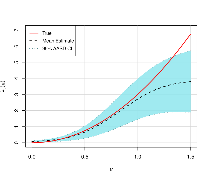
(a) $\pi^{E}=0.3,n=100,m=5$

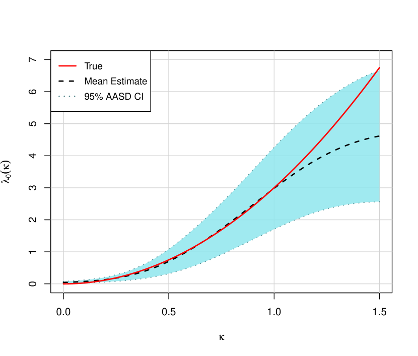
(b) $\pi^{E}=0.7,n=100,m=5$

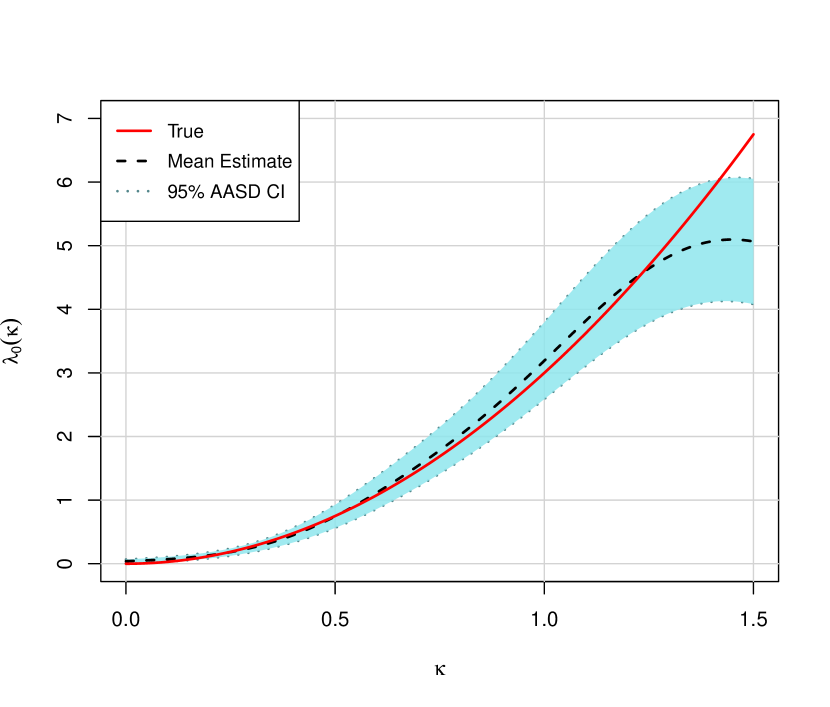
(c) $\pi^{E}=0.3,n=1000,m=10$

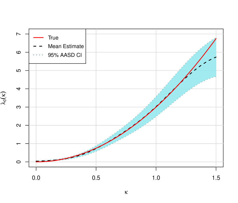
(d) $\pi^{E}=0.7,n=1000,m=10$

Figure 1: Figures of the baseline hazard functions on a grid of $\kappa$ values. Each plot includes the true baseline hazard curve (solid red line), the mean estimated baseline hazard curve (dashed black line) and area bound by the 95% pointwise confidence interval generated using AASD (coloured region).

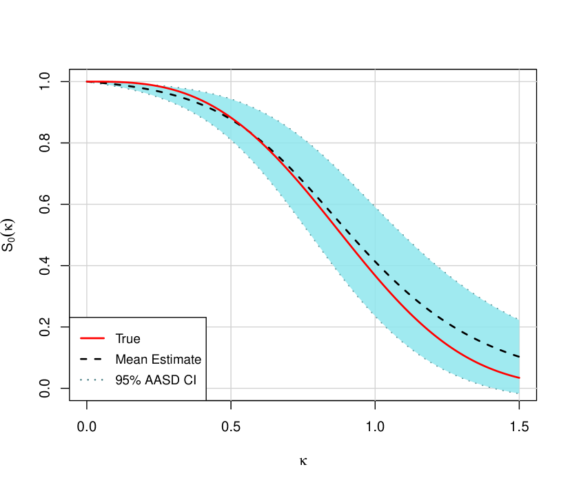
(a) $\pi^{E}=0.3,n=100,m=5$

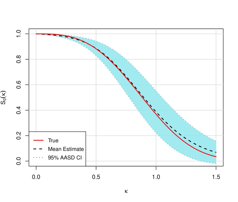
(b) $\pi^{E}=0.7,n=100,m=5$

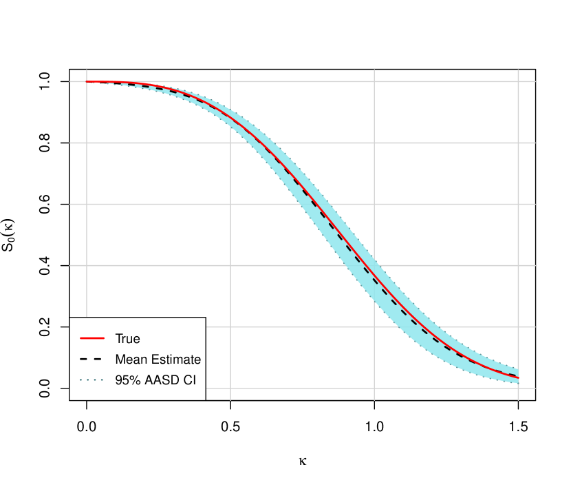
(c) $\pi^{E}=0.3,n=1000,m=10$

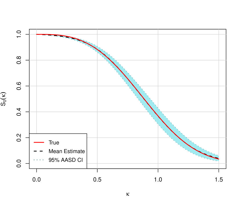
(d) $\pi^{E}=0.7,n=1000,m=10$

Figure 2: Figures of the baseline survival functions on a grid of $\kappa$ values. Each plot includes the true baseline survival curve (solid red line), the mean estimated baseline survival curve (dashed black line) and area bound by the 95% pointwise confidence interval generated using AASD (coloured region).

Figures 1 and 2 contain plots illustrating the mean estimated baseline hazard, $\lambda_{0}(\kappa)$, and the mean estimated baseline survival, $S_{0}(\kappa)$, against $\kappa$ for varying proportions of exact event times and sample sizes. The results reveal that the averages of the estimated baseline functions closely align with the true baseline functions especially when $\kappa\leq 1$. An improvement in the accuracy of these estimated baseline functions can be observed over a longer range with an increase in either the proportion of exact failure times or the sample size. In addition, the widths of the pointwise AASD CIs significantly decrease with an increase in sample size, highlighting the improved precision of the estimation. Notably in Figure 1, the deviations between the true and mean estimated baseline hazards towards the ends of the curves are attributed to the use of a mixture of Gaussian basis functions in estimating the monotonic Weibull hazard.

Note that in the special case involving a single time-varying covariate as defined in (17), the expression for the failure times in (3) can be simplified as follows

$$T_{i}=\begin{cases}e^{\boldsymbol{x_{i}}\beta+\varepsilon_{i}}&\text{if }0<t_{i}<\tau_{i};\\ e^{\gamma}(e^{\boldsymbol{x_{i}}\beta+\varepsilon}-\tau_{i})+\tau_{i}&\text{if }t_{i}\geq\tau_{i}.\end{cases}$$ (18)

Unlike AFT models with only time-fixed covariates, we will need to consider the values of $\tau_{i}$ as well and thus the estimated coefficients cannot be as easily interpreted. Therefore, we assess the effects of the time-fixed and time-varying covariates based on the survival functions instead. First let us assess the effect of a unit increase in a particular time-fixed covariate. Assuming that the event history of the time-varying covariates is given, the ratio between the survival functions depicting the effect of increasing $x_{1}$ by one unit is given below

$$\frac{S(t|x_{1}^{*}=x_{1}+1,x_{2},\tilde{\boldsymbol{z}}(t),\tau)}{S(t|x_{1},x_{2},\tilde{\boldsymbol{z}}(t),\tau)} =\frac{S_{0}\left(e^{-\{x_{1}^{*}\beta_{1}+x_{2}\beta_{2}\}}\{e^{-\gamma}(t-\tau)+\tau\}\right)}{S_{0}\left(e^{-\boldsymbol{x}\boldsymbol{\beta}}\{e^{-\gamma}(t-\tau)+\tau\}\right)}$$ (19)

$$=\frac{S_{0}\left(e^{-(\boldsymbol{x}\boldsymbol{\beta}+\beta_{1})}\{e^{-\gamma}(t-\tau)+\tau\}\right)}{S_{0}\left(e^{-\boldsymbol{x}\boldsymbol{\beta}}\{e^{-\gamma}(t-\tau)+\tau\}\right)}.$$

With $\tau=0.2$ designated for demonstration purposes, Figure 3 contains the predicted survival curves that allow us to compare the effect of a unit increase in $x_{1}$ in our simulation study. This figure illustrates that increasing $x_{1}$ by one unit positively affects the predicted survival probabilities. This is as expected as $\beta_{1}^{0}$ is positively valued at 1. Additionally, the computed survival ratios between the two curves across all $t$, in accordance with the reciprocal of (19) (for ease of understanding), is also provided.

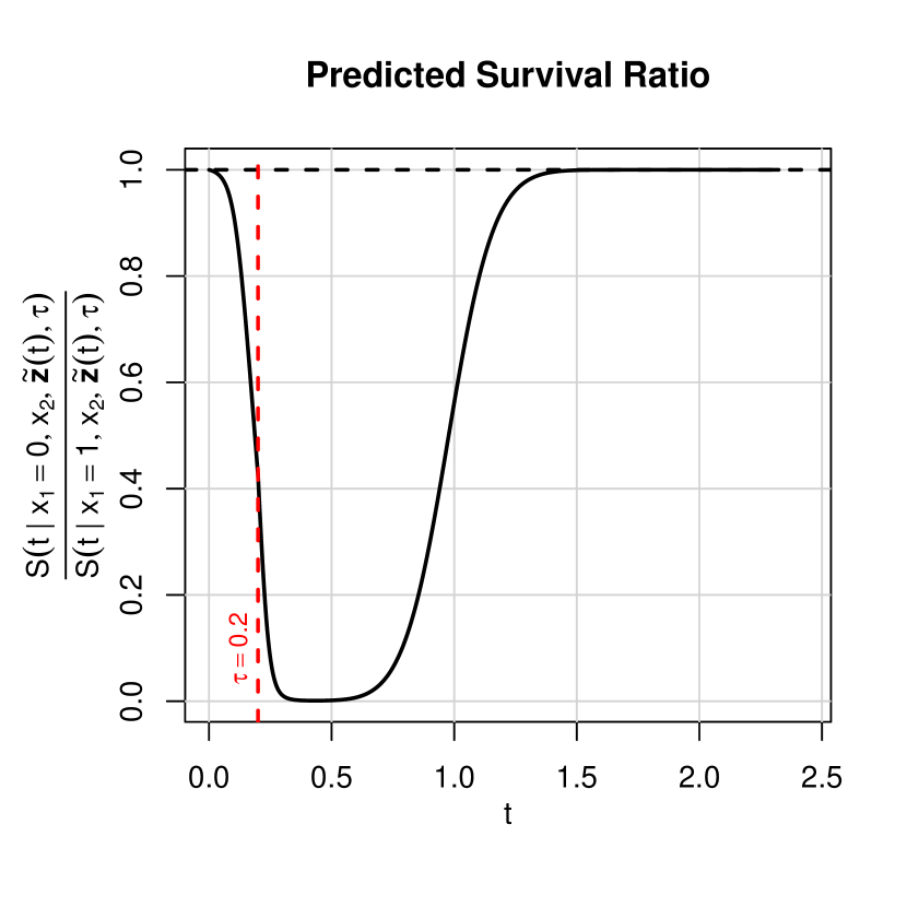
Figure 3: Effect of a time-fixed covariate on survival probability and survival time: plots of two predicted survival curves ($S(t|x_{1}=1,x_{2},\tilde{\boldsymbol{z}}(t),\tau=0.2)$ vs $S(t|x_{1}=0,x_{2},\tilde{\boldsymbol{z}}(t),\tau=0.2)$) and the ratio between these two survival curves, based on a single generated sample with settings ${\pi}^{E}=0.7$, $n=1000$, $m=10$. The value of $x_{2}$ adopts the median of $\boldsymbol{x}_{2}$ of the generated sample. The time-varying covariate $\tilde{\boldsymbol{z}}(t)$ is defined in (17).

Similarly, comparisons for an individual who receives treatment at time $\tau$ versus not receiving any treatment can also be made. The ratio between the survival functions for such a case is quantified by the ratio given below

$$\frac{S(t|\boldsymbol{x},\tilde{\boldsymbol{z}}(t),\tau)}{S(t|\boldsymbol{x},\tilde{\boldsymbol{z}}(t)=\boldsymbol{0})} =\frac{S_{0}\left(e^{-\boldsymbol{x}\boldsymbol{\beta}}\{e^{-\gamma}(t-\tau)+\tau\}\right)}{S_{0}\left(te^{-\boldsymbol{x}\boldsymbol{\beta}}\right)}.$$ (20)

In Figure 4, the predicted survival curves allow us to compare the effect of having time-varying treatment versus not having time-varying treatment. Here, we still choose $\tau=0.2$. The plot indicates that the predicted survival probabilities worsen post-treatment, which coincides with $\gamma^{0}$ being negatively valued at $-0.5$. Once again, we provide the computed survival ratios between the two curves across all $t$, in accordance with (20).

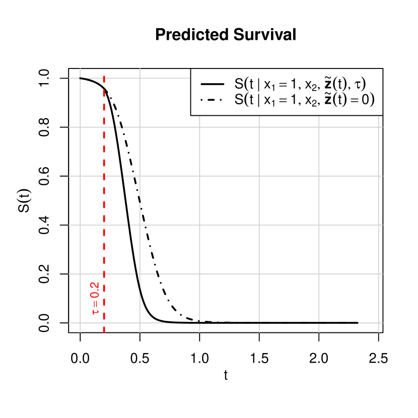
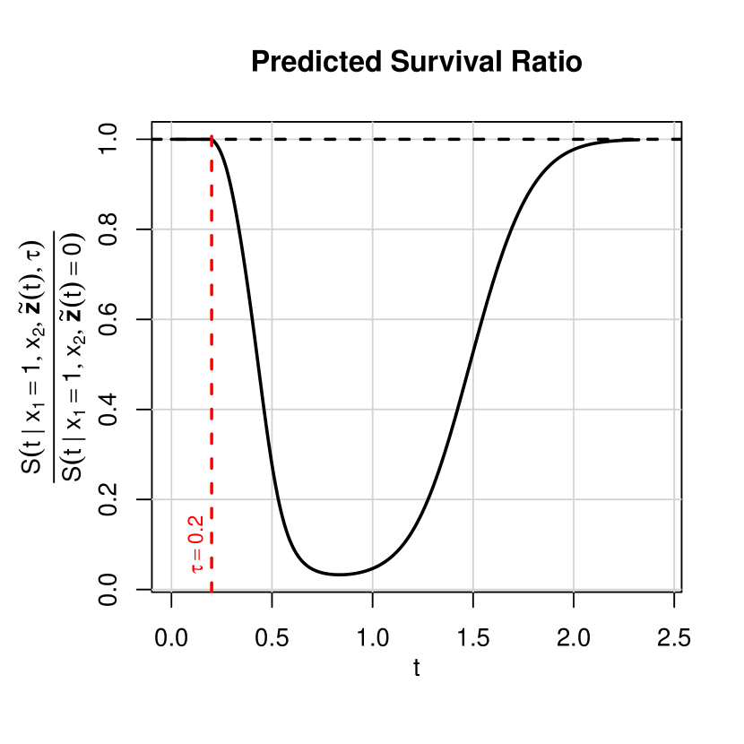
Figure 4: Effect of a time-varying covariate on survival probability and survival time: plots of two predicted survival curves ($S(t|x_{1}=1,x_{2},\tilde{\boldsymbol{z}}(t),\tau=0.2)$ vs $S(t|x_{1}=1,x_{2},\tilde{\boldsymbol{z}}(t)=\boldsymbol{0}))$ and the ratio between these two survival curves, based on a generated sample with settings ${\pi}^{E}=0.7$, $n=1000$, $m=10$. The value of $x_{2}$ adopts the median of $\boldsymbol{x}_{2}$ of the generated sample. The time-varying covariate $\tilde{\boldsymbol{z}}(t)$ is defined in (17).

6 Application

The WBRTMel trial is a multinational, open-label, phase III randomised controlled trial that compared whole brain radiotherapy (WBRT) to observation (control). Eligible patients were randomised after first local treatment (surgical excision and/or stereotactic irradiation treatment) of 1 to 3 melanoma brain metastases. The primary outcome was the proportion of patients with distant intracranial failure as determined by magnetic resonance imaging within 12 months from the randomisation date. The study concluded that adjuvant WBRT does not provide evidence of clinical benefit in terms of distant intracranial control (Hong et al.,, 2019). This result was based on the non-statistically significant effect of WBRT on the primary outcome using logistic regression as planned in the statistical analysis plan (Lo et al.,, 2019). We re-analysed the trial data using our new approach to evaluate the effectiveness of WBRT treatment on time to intracranial failure.

The dataset considered here includes basic demographic information and medical records for 207 patients (100 patients were randomly assigned to the WBRT arm and 107 patients to the observation arm), totaling 1187 longitudinal entries. Of the full cohort, 86 patients (41.5%) experienced interval-censored failure times, 28 patients (13.5%) experienced left-censored failure times, and the remaining 93 (45%) of time-to-event records are right-censored. Notably, there were no exactly observed events in this dataset.

We incorporated five time-fixed covariates: the treatment group (observation or whole-brain radiation therapy (WBRT)), gender (female or male), presence of extracranial disease at baseline (absent or present), number of melanoma brain metastases (MBM) (1 or 2-3) and age (in years, rounded off to one decimal place). In addition, one time-varying (dichotomous) covariate is considered in this application, which is the use of systemic therapy (no or yes), where the values are constant between any two consecutive examinations. Here, the number of longitudinal entries for the patients varies between 1 and 44. Out of 207 patients, 12 have their longitudinal records of systemic therapy use partially missing. These missing values are imputed as ”no” in this study, assuming patients did not receive systemic therapy during these periods.

A summary of the variables is shown in Table 3. Two-thirds of the patients are male and the average age is 61.3 (SD=12.2). At the time of randomisation two-thirds of the patients had extracranial disease and nearly 40% had more than one MBM. With regards to the time-varying covariate, 55.6% of the patients had received systemic therapy at some point in time during the study. These patients received systemic therapy for 39.6% of the follow-up duration on average.

Table 3: Covariates of interest in the MBM dataset

Covariates	Levels	# Patients	Percentage
Treatment	Observation (reference group)	107	51.7%
	WBRT	100	48.3%
Gender	Female (reference group)	69	33.3%
	Male	138	66.7%
Number of MBM	$=1$ (reference group)	127	61.4%
	$>1$	80	38.6%
Extracranial disease	Absent (reference group)	68	32.9%
	Present	139	67.1%
Covariates		Mean (median)	Standard deviation
Age	(in years)	61.3 (63.3)	12.2
Covariates	Levels	# Patients (# records)	Average duration percentage
Systemic therapy	No	115 (1029)	–
	Yes	92 (158)	39.6%

To analyse the dataset obtained from the WBRTMel trial, we once again utilised the algorithm based on the model formulation outlined in Section 3 and the strategy detailed in Section 4. For this analysis, we chose to adopt 5 basis functions with their locations determined using a quantile function. Using more than 5 knots resulted in a higher number of active constraints. The optimization process was halted once the change in the estimates of the model parameters were within a tolerance level of $10^{-6}$ and the smoothing parameters converged. Specifically for this dataset, the algorithm took 3.6 minutes to converge. The results obtained, including the estimated coefficients and their associated standard errors, are presented in Table 4. Since the estimators for the regression and basis coefficients are asymptotically normal, we also provide the Wald test statistics and p-values in the table. From the table, it is evident that all covariates are significant, except for the presence of extracranial disease at baseline. To further assess the effects of the time-fixed and time-varying covariates included in our model, it is advisable to examine the predicted survival curves and the ratios of survival curves quantified according to (19) or (20).

Table 4: Results for the covariates in the MBM dataset

	$\hat{\beta}$	se($\hat{\beta}$)	Wald statistic	P-value
Treatment (WBRT vs observation)	0.574	0.152	3.773	$<0.001$
Gender (male vs female)	-0.473	0.143	-3.297	$<0.001$
Number of MBM ($>1$ vs $=1$)	-0.705	0.147	-4.780	$<0.001$
Extracranial disease (present vs absent)	-0.037	0.141	-0.260	0.795
Age (in years)	-0.025	0.002	-11.058	$<0.001$
	$\hat{\gamma}$	se($\hat{\gamma}$)	Wald statistic	P-value
Systemic therapy (yes vs no)	0.483	0.246	1.967	0.049

As an illustration, Figure 5 displays plots of predicted distant intracranial free survival (in years) for a time-fixed covariate of interest, treatment (WBRT vs observation), under four different scenarios of the time-varying covariate, systemic therapy. For illustrative purposes, we designate $\tau=2$ years (the minimum follow-up time of the study) as the transition point for the time-varying systemic therapy. More explicitly, Figure 5(a) corresponds to the situation when a patient does not receive systemic therapy throughout the follow-up period; Figure 5(b) depicts the case where a patient receives systemic therapy after but not before $\tau=2$; Figure 5(c) showcases the scenario when a patient receives systemic therapy before but not after $\tau=2$; Figure 5(d) demonstrates the case that a patient receives systemic therapy throughout the follow-up period. For each of the predicted survival plots, the time-fixed covariates not of interest for prediction purposes are configured based on the following default settings: gender as female, number of MBM as $>1$, extracranial disease as present and age as its median value (63.3).

Figure 5 illustrates that patients who received WBRT generally have a larger median time to distant intracranial control, compared to those in the observation group, in the four scenarios considered with respect to systemic therapy status. Hence, WBRT appears to delay the time to intracranial failure in this study, which can also be generally concluded from the corresponding positively valued regression coefficient. Similar analyses can be performed for the other significant time-fixed covariates, the predicted survival curves of which are provided in the supplementary material.

In terms of receiving systemic therapy, a time-varying covariate, one can interpret that receiving systemic therapy generally results in longer survival times due to the positively valued coefficient. By further observing the plots in Figure 5, within the same treatment group (either WBRT or observation), we conclude that those who receive systemic therapy continuously throughout the follow-up period (Figure 5(d)) exhibit the longest distant intracranial failure. On the other hand, those who never receive systemic therapy demonstrate the shortest survival time. Comparing Figure 5(b) and Figure 5(c), it is notable that up to $t=4$, the survival probabilities of patients who receive systemic therapy between $t=0$ and $t=2$ consistently display higher survival probabilities than those who receive systemic therapy between $t=2$ and $t=4$. In conclusion, time-varying systemic therapy has a beneficial impact on the survival probabilities (and/or survival times) of patients. Administering systemic therapy earlier and for longer durations correlates with higher rate of distant intracranial control for patients.

Our conclusion offers new insights regarding the efficacy of WBRT in treating advanced melanoma patients. These results, obtained from an AFT model that was adjusted with systemic therapy as a time-varying covariate, complement the main findings reported by Hong et al., (2019), which were based on standard logistic regression and the Fine and Gray model without covariate adjustment. We refrain from providing a detailed numerical interpretation of the plots, as the effects of covariates on survival probabilities or duration are nonlinear over time. However, the ratios of survival probabilities in Figure 5 can be derived in a similar manner to (19) and (20), if necessary. Additional predictive plots can be found in the supplementary material.

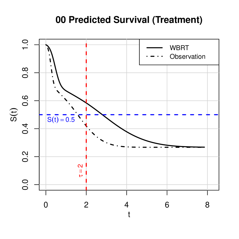
(a) No systemic therapy throughout follow-up period

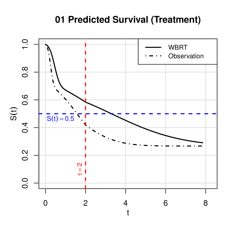
(b) Given systemic therapy after but not before $\tau=2$

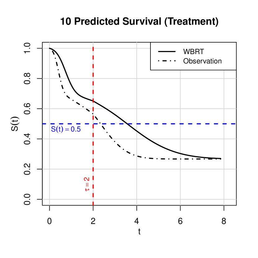
(c) Given systemic therapy before but not after $\tau=2$

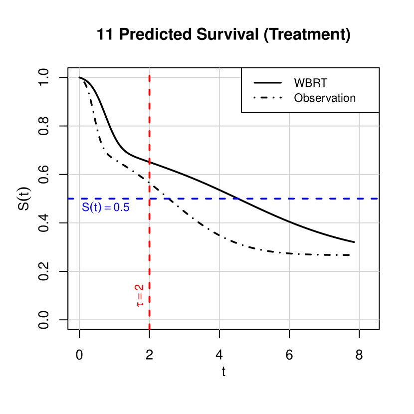
(d) Given systemic therapy throughout follow-up period

Figure 5: Predicted distant intracranial control rate (during follow-up time in years) for the time-fixed covariate, treatment (WBRT vs observation), assuming four different scenarios of the time-varying covariate: systemic therapy.

7 Discussion

Accelerated failure time models allow for the modelling of survival data where the failure times are either accelerated or decelerated by a multiplicative factor in the presence of several covariates. In this paper, we considered semiparametric AFT models and provided a pathway to estimating such models with time-varying covariates under partly interval censoring, previously unavailable in the literature.

In our approach, we selected Gaussian basis functions to approximate the unknown baseline hazard, which also help avoid numerical instabilities. Additionally, a roughness penalty was introduced to construct a smooth approximation of the baseline hazard function. We proposed an algorithm alternating between pseudo-Newton and MI steps to carry out constrained optimisation. Together with a marginal likelihood-based automatic smoothing parameter selection, the algorithm successfully obtained the required maximum penalised likelihood estimates. In Section 4.4, the stated asymptotic results allow for statistical inference to be carried out even in the presence of active constraints. The simulation results presented in Section 5 show that the proposed algorithm provides satisfactory results. In Section 6, our approach was further illustrated using a dataset on melanoma brain metastases. In both the simulation and application sections, we provided examples of survival ratios and predictive survival plots to help assess the effects of the various time-fixed and time-varying covariates in the model considered.

With regards to computational times, each replication in the simulation study with a small sample size ($n=100$) required 15 seconds on average to optimise. In comparison, the dataset from the WBRTMel trial ($n=207$) required 3.5 minutes to optimise. On the other hand, each replication in the simulation study with a large sample size ($n=1000$) required an average of 5 minutes to optimise. The R code used for the simulation studies and data analysis in this paper is publicly available at https://github.com/aishwarya-b22/AFT_TVC_PIC, where we provide a comprehensive vignette for fitting the model. In future work, we aim to reduce computational times using tools such as Rcpp in order to ease the implementation of accelerated failure time models.

The methodology proposed in the paper can be easily extended to a joint AFT model capturing both survival time and longitudinal predictors. The integration of longitudinal and survival data through joint models is especially pertinent in numerous observational studies. In such cases, repeated measurements from longitudinal biomarkers often exhibit significant associations with time-to-event outcomes or overall survival. This approach specifically models the correlation between longitudinal data and time-to-event data and can account for the potential measurement error in the biomarkers.

Data Availability Statement

The WBRTMel dataset may be accessed upon reasonable request from the Melanoma Institute Australia.

Supplementary Materials for

by Aishwarya Bhaskaran, Ding Ma, Benoit Liquet, Angela Hong, Serigne N Lo, Stephane Heritier and Jun Ma

Appendix A Vector and matrix representations for the gradients, Hessians and pseudo Hessians

A.1 Notation

Let us define

$$d_{\boldsymbol{\beta}}P(\boldsymbol{\beta},\boldsymbol{\gamma},\boldsymbol{\theta}),\quad D_{\boldsymbol{\beta}}P(\boldsymbol{\beta},\boldsymbol{\gamma},\boldsymbol{\theta}),\quad\nabla_{\boldsymbol{\beta}}P(\boldsymbol{\beta},\boldsymbol{\gamma},\boldsymbol{\theta})\quad\text{and}\quad H_{\boldsymbol{\beta}}P(\boldsymbol{\beta},\boldsymbol{\gamma},\boldsymbol{\theta}),$$

as the vector of differentials, derivative vector, gradient and Hessian of the penalized log-likelihood, $P(\boldsymbol{\beta},\boldsymbol{\gamma},\boldsymbol{\theta})$, with respect to $\boldsymbol{\beta}$. In addition, let

$$H^{-}_{\boldsymbol{\beta}}P(\boldsymbol{\beta},\boldsymbol{\gamma},\boldsymbol{\theta}),$$

denote the pseudo Hessian of the penalized log-likelihood with respect to $\boldsymbol{\beta}$. The pseudo Hessian is obtained from the original expression of the Hessian by only extracting the negative terms.

The notation in this subsection applies to other model parameters as well.

A.2 Expressions with respect to $\boldsymbol{\beta}$

Firstly note that,

$$d_{\boldsymbol{\beta}}\kappa_{i}(y_{i}) =e^{-\boldsymbol{X}_{i}\boldsymbol{\beta}}\int_{0}^{y_{i}}e^{-z_{i}(s)\boldsymbol{\gamma}}ds\hskip 2.84526ptd(-\boldsymbol{X}_{i}\boldsymbol{\beta})$$

$$=-\kappa_{i}(y_{i})\boldsymbol{X}_{i}d\boldsymbol{\beta},$$

and

$$d_{\boldsymbol{\beta}}\exp\{-\Lambda_{0}(\kappa_{i}(y_{i}))\} =-\exp\{-\Lambda_{0}(\kappa_{i}(y_{i}))\}d\{\Lambda_{0}(\kappa_{i}(y_{i}))\}$$

$$=-\exp\{-\Lambda_{0}(\kappa_{i}(y_{i}))\}\lambda_{0}(\kappa_{i}(y_{i}))d\{\kappa_{i}(y_{i})\}$$

$$=\exp\{-\Lambda_{0}(\kappa_{i}(y_{i}))\}\lambda_{0}(\kappa_{i}(y_{i}))\kappa_{i}(y_{i})\boldsymbol{X}_{i}d\boldsymbol{\beta}.$$

A.2.1 Gradient with respect to $\boldsymbol{\beta}$

The gradient of $P(\boldsymbol{\beta},\boldsymbol{\gamma},\boldsymbol{\theta})$ with respect to $\boldsymbol{\beta}$ can be derived as,

$$\nabla_{\boldsymbol{\beta}}P(\boldsymbol{\beta},\boldsymbol{\gamma},\boldsymbol{\theta})=D_{\boldsymbol{\beta}}P(\boldsymbol{\beta},\boldsymbol{\gamma},\boldsymbol{\theta})^{T},$$

which can be shown to be,

$$D_{\boldsymbol{\beta}}P(\boldsymbol{\beta},\boldsymbol{\gamma},\boldsymbol{\theta})^{T}$$

$$=\sum_{i=1}^{n}\boldsymbol{X}_{i}^{T}\Bigg{(}\delta_{i}\left\{-\frac{\lambda_{0}^{{}^{\prime}}(\kappa_{i}(y_{i}))\kappa_{i}(y_{i})}{\lambda_{0}(\kappa_{i}(y_{i}))}-1+\lambda_{0}(\kappa_{i}(y_{i}))\kappa_{i}(y_{i})\right\}+\delta^{R}_{i}\lambda_{0}(\kappa_{i}(y_{i}^{L}))\kappa_{i}(y_{i}^{L})\Big{)}$$

$$\qquad-\delta^{L}_{i}\left[\frac{\exp\{-\Lambda_{0}(\kappa_{i}(y_{i}^{R}))\}\lambda_{0}(\kappa_{i}(y_{i}^{R}))\kappa_{i}(y_{i}^{R})}{1-\exp\{-\Lambda_{0}(\kappa_{i}(y_{i}^{R}))\}}\right]$$

$$\qquad+\delta^{I}_{i}\left[\frac{\exp\{-\Lambda_{0}(\kappa_{i}(y_{i}^{L}))\}\lambda_{0}(\kappa_{i}(y_{i}^{L}))\kappa_{i}(y_{i}^{L})-\exp\{-\Lambda_{0}(\kappa_{i}(y_{i}^{R}))\}\lambda_{0}(\kappa_{i}(y_{i}^{R}))\kappa_{i}(y_{i}^{R})}{\exp\{-\Lambda_{0}(\kappa_{i}(y_{i}^{L}))\}-\exp\{-\Lambda_{0}(\kappa_{i}(y_{i}^{R}))\}}\right]\Bigg{)}.$$

A.2.2 Hessian with respect to $\boldsymbol{\beta}$

Note that

$$H_{\boldsymbol{\beta}}P(\boldsymbol{\beta},\boldsymbol{\gamma},\boldsymbol{\theta})=D_{\boldsymbol{\beta}}\left(D_{\boldsymbol{\beta}}P(\boldsymbol{\beta},\boldsymbol{\gamma},\boldsymbol{\theta})^{T}\right).$$

Then the Hessian of $P(\boldsymbol{\beta},\boldsymbol{\gamma},\boldsymbol{\theta})$ with respect to $\boldsymbol{\beta}$ can be shown to be,

$$H_{\boldsymbol{\beta}}P(\boldsymbol{\beta},\boldsymbol{\gamma},\boldsymbol{\theta})$$

$$=\sum_{i=1}^{n}\boldsymbol{X}_{i}^{T}\Bigg{[}\delta_{i}\Bigg{(}\left[\frac{\lambda_{0}(\kappa_{i}(y_{i}))\lambda_{0}^{{}^{\prime\prime}}(\kappa_{i}(y_{i}))-\{\lambda_{0}^{{}^{\prime}}(\kappa_{i}(y_{i}))\}^{2}}{\{\lambda_{0}(\kappa_{i}(y_{i}))\}^{2}}-\lambda_{0}^{{}^{\prime}}(\kappa_{i}(y_{i}))\right]\{\kappa_{i}(y_{i})\}^{2}+\left\{\frac{\lambda_{0}^{{}^{\prime}}(\kappa_{i}(y_{i}))}{\lambda_{0}(\kappa_{i}(y_{i}))}-\lambda_{0}(\kappa_{i}(y_{i}))\right\}\kappa_{i}(y_{i})\Bigg{)}$$

$$\qquad-\delta^{R}_{i}\{\lambda_{0}^{{}^{\prime}}(\kappa_{i}(y_{i}^{L}))\kappa_{i}(y_{i}^{L})+\lambda_{0}(\kappa_{i}(y_{i}^{L}))\}\kappa_{i}(y_{i}^{L})-\delta^{L}_{i}\Bigg{\{}\Bigg{(}\frac{\exp\{-\Lambda_{0}(\kappa_{i}(y_{i}^{R}))\}\left[\{\lambda_{0}(\kappa_{i}(y_{i}^{R}))\}^{2}-\lambda_{0}^{{}^{\prime}}(\kappa_{i}(y_{i}^{R}))\right]}{1-\exp\{-\Lambda_{0}(\kappa_{i}(y_{i}^{R}))\}}$$

$$\qquad\quad+\left[\frac{\exp\{-\Lambda_{0}(\kappa_{i}(y_{i}^{R}))\}\lambda_{0}(\kappa_{i}(y_{i}^{R}))}{1-\exp\{-\Lambda_{0}(\kappa_{i}(y_{i}^{R}))\}}\right]^{2}\Bigg{)}\{\kappa_{i}(y_{i}^{R})\}^{2}-\left[\frac{\exp\{-\Lambda_{0}(\kappa_{i}(y_{i}^{R}))\}\lambda_{0}(\kappa_{i}(y_{i}^{R}))}{1-\exp\{-\Lambda_{0}(\kappa_{i}(y_{i}^{R}))\}}\right]\kappa_{i}(y_{i}^{R})\Bigg{\}}$$

$$\qquad+\delta^{I}_{i}\Bigg{\{}\Bigg{(}\frac{\exp\{-\Lambda_{0}(\kappa_{i}(y_{i}^{L}))\}\left[\{\lambda_{0}(\kappa_{i}(y_{i}^{L}))\}^{2}-\lambda_{0}^{{}^{\prime}}(\kappa_{i}(y_{i}^{L}))\right]}{\exp\{-\Lambda_{0}(\kappa_{i}(y_{i}^{L}))\}-\exp\{-\Lambda_{0}(\kappa_{i}(y_{i}^{R}))\}}-\left[\frac{\exp\{-\Lambda_{0}(\kappa_{i}(y_{i}^{L}))\}\lambda_{0}(\kappa_{i}(y_{i}^{L}))}{\exp\{-\Lambda_{0}(\kappa_{i}(y_{i}^{L}))\}-\exp\{-\Lambda_{0}(\kappa_{i}(y_{i}^{R}))\}}\right]^{2}\Bigg{)}\{\kappa_{i}(y_{i}^{L})\}^{2}$$

$$\qquad\quad-\left[\frac{\exp\{-\Lambda_{0}(\kappa_{i}(y_{i}^{L}))\}\lambda_{0}(\kappa_{i}(y_{i}^{L}))}{\exp\{-\Lambda_{0}(\kappa_{i}(y_{i}^{L}))\}-\exp\{-\Lambda_{0}(\kappa_{i}(y_{i}^{R}))\}}\right]\kappa_{i}(y_{i}^{L})-\Bigg{(}\frac{\exp\{-\Lambda_{0}(\kappa_{i}(y_{i}^{R}))\}\left[\{\lambda_{0}(\kappa_{i}(y_{i}^{R}))\}^{2}-\lambda_{0}^{{}^{\prime}}(\kappa_{i}(y_{i}^{R}))\right]}{\exp\{-\Lambda_{0}(\kappa_{i}(y_{i}^{L}))\}-\exp\{-\Lambda_{0}(\kappa_{i}(y_{i}^{R}))\}}$$

$$\qquad\quad+\left[\frac{\exp\{-\Lambda_{0}(\kappa_{i}(y_{i}^{R}))\}\lambda_{0}(\kappa_{i}(y_{i}^{R}))}{\exp\{-\Lambda_{0}(\kappa_{i}(y_{i}^{L}))\}-\exp\{-\Lambda_{0}(\kappa_{i}(y_{i}^{R}))\}}\right]^{2}\Bigg{)}\{\kappa_{i}(y_{i}^{R})\}^{2}+\left[\frac{\exp\{-\Lambda_{0}(\kappa_{i}(y_{i}^{R}))\}\lambda_{0}(\kappa_{i}(y_{i}^{R}))}{\exp\{-\Lambda_{0}(\kappa_{i}(y_{i}^{L}))\}-\exp\{-\Lambda_{0}(\kappa_{i}(y_{i}^{R}))\}}\right]\kappa_{i}(y_{i}^{R})$$

$$\qquad\quad+2\left(\frac{\exp\{-\Lambda_{0}(\kappa_{i}(y_{i}^{L}))\}\lambda_{0}(\kappa_{i}(y_{i}^{L}))\kappa_{i}(y_{i}^{L})\exp\{-\Lambda_{0}(\kappa_{i}(y_{i}^{R}))\}\lambda_{0}(\kappa_{i}(y_{i}^{R}))\kappa_{i}(y_{i}^{R})}{\left[\exp\{-\Lambda_{0}(\kappa_{i}(y_{i}^{L}))\}-\exp\{-\Lambda_{0}(\kappa_{i}(y_{i}^{R}))\}\right]^{2}}\right)\Bigg{\}}\Bigg{]}\boldsymbol{X}_{i}.$$

A.2.3 Pseudo Hessian with respect to $\boldsymbol{\beta}$

Subsequently, the pseudo Hessian of $P(\boldsymbol{\beta},\boldsymbol{\gamma},\boldsymbol{\theta})$ with respect to $\boldsymbol{\beta}$ is,

$$H^{-}_{\boldsymbol{\beta}}P(\boldsymbol{\beta},\boldsymbol{\gamma},\boldsymbol{\theta})$$

$$=-\sum_{i=1}^{n}\boldsymbol{X}_{i}^{T}\Bigg{[}\delta_{i}\Bigg{[}\left\{\frac{\lambda_{0}^{{}^{\prime}}(\kappa_{i}(y_{i}))\kappa_{i}(y_{i})}{\lambda_{0}(\kappa_{i}(y_{i}))}\right\}^{2}+\lambda_{0}(\kappa_{i}(y_{i}))\kappa_{i}(y_{i})\Bigg{]}+\delta^{R}_{i}\lambda_{0}(\kappa_{i}(y_{i}^{L}))\kappa_{i}(y_{i}^{L})$$

$$\qquad+\delta^{L}_{i}\Bigg{\{}\Bigg{(}\frac{\exp\{-\Lambda_{0}(\kappa_{i}(y_{i}^{R}))\}\{\lambda_{0}(\kappa_{i}(y_{i}^{R}))\}^{2}}{1-\exp\{-\Lambda_{0}(\kappa_{i}(y_{i}^{R}))\}}+\left[\frac{\exp\{-\Lambda_{0}(\kappa_{i}(y_{i}^{R}))\}\lambda_{0}(\kappa_{i}(y_{i}^{R}))}{1-\exp\{-\Lambda_{0}(\kappa_{i}(y_{i}^{R}))\}}\right]^{2}\Bigg{)}\{\kappa_{i}(y_{i}^{R})\}^{2}\Bigg{\}}$$

$$\qquad+\delta^{I}_{i}\Bigg{\{}\left[\frac{\exp\{-\Lambda_{0}(\kappa_{i}(y_{i}^{L}))\}\lambda_{0}(\kappa_{i}(y_{i}^{L}))}{\exp\{-\Lambda_{0}(\kappa_{i}(y_{i}^{L}))\}-\exp\{-\Lambda_{0}(\kappa_{i}(y_{i}^{R}))\}}\right]^{2}\{\kappa_{i}(y_{i}^{L})\}^{2}+\left[\frac{\exp\{-\Lambda_{0}(\kappa_{i}(y_{i}^{L}))\}\lambda_{0}(\kappa_{i}(y_{i}^{L}))}{\exp\{-\Lambda_{0}(\kappa_{i}(y_{i}^{L}))\}-\exp\{-\Lambda_{0}(\kappa_{i}(y_{i}^{R}))\}}\right]\kappa_{i}(y_{i}^{L})$$

$$\qquad\quad+\Bigg{(}\frac{\exp\{-\Lambda_{0}(\kappa_{i}(y_{i}^{R}))\}\{\lambda_{0}(\kappa_{i}(y_{i}^{R}))\}^{2}}{\exp\{-\Lambda_{0}(\kappa_{i}(y_{i}^{L}))\}-\exp\{-\Lambda_{0}(\kappa_{i}(y_{i}^{R}))\}}+\left[\frac{\exp\{-\Lambda_{0}(\kappa_{i}(y_{i}^{R}))\}\lambda_{0}(\kappa_{i}(y_{i}^{R}))}{\exp\{-\Lambda_{0}(\kappa_{i}(y_{i}^{L}))\}-\exp\{-\Lambda_{0}(\kappa_{i}(y_{i}^{R}))\}}\right]^{2}\Bigg{)}\{\kappa_{i}(y_{i}^{R})\}^{2}\Bigg{]}\boldsymbol{X}_{i}.$$

A.3 Expressions with respect to $\boldsymbol{\gamma}$

Next note that,

$$d_{\boldsymbol{\gamma}}\kappa_{i}(y_{i}) =e^{-\boldsymbol{X}_{i}\boldsymbol{\beta}}\int_{0}^{y_{i}}e^{-z_{i}(s)\boldsymbol{\gamma}}d(-z_{i}(s)\boldsymbol{\gamma})ds$$

$$=-e^{-\boldsymbol{X}_{i}\boldsymbol{\beta}}\int_{0}^{y_{i}}e^{-z_{i}(s)\boldsymbol{\gamma}}z_{i}(s)dsd\boldsymbol{\gamma},$$

$$D_{\boldsymbol{\gamma}}\kappa_{i}(y_{i}) =-e^{-\boldsymbol{X}_{i}\boldsymbol{\beta}}\int_{0}^{y_{i}}e^{-z_{i}(s)\boldsymbol{\gamma}}z_{i}(s)ds,$$

and

$$D_{\boldsymbol{\gamma}}\{D_{\boldsymbol{\gamma}}\kappa_{i}(y_{i})^{T}\}=e^{-\boldsymbol{X}_{i}\boldsymbol{\beta}}\int_{0}^{y_{i}}e^{-z_{i}(s)\boldsymbol{\gamma}}z_{i}(s)^{T}z_{i}(s)ds.$$

Also note that,

$$d\exp\{-\Lambda_{0}(\kappa_{i}(y_{i}))\}=-\exp\{-\Lambda_{0}(\kappa_{i}(y_{i}))\}\lambda_{0}(\kappa_{i}(y_{i}))d_{\boldsymbol{\gamma}}\kappa_{i}(y_{i}).$$

A.3.1 Gradient with respect to $\boldsymbol{\gamma}$

The gradient of $P(\boldsymbol{\beta},\boldsymbol{\gamma},\boldsymbol{\theta})$ with respect to $\boldsymbol{\gamma}$ can be derived as,

$$\nabla_{\boldsymbol{\gamma}}P(\boldsymbol{\beta},\boldsymbol{\gamma},\boldsymbol{\theta})=D_{\boldsymbol{\gamma}}P(\boldsymbol{\beta},\boldsymbol{\gamma},\boldsymbol{\theta})^{T}\,$$

which can be shown to be,

$$D_{\boldsymbol{\gamma}}P(\boldsymbol{\beta},\boldsymbol{\gamma},\boldsymbol{\theta})^{T}$$

$$=\sum_{i=1}^{n}\Bigg{(}-\delta_{i}z_{i}(y_{i})^{T}+\delta_{i}\left\{\frac{\lambda_{0}^{{}^{\prime}}(\kappa_{i}(y_{i}))}{\lambda_{0}(\kappa_{i}(y_{i}))}-\lambda_{0}(\kappa_{i}(y_{i}))\right\}D_{\boldsymbol{\gamma}}\kappa_{i}(y_{i})^{T}-\delta^{R}_{i}\lambda_{0}(\kappa_{i}(y_{i}^{L}))D_{\boldsymbol{\gamma}}\kappa_{i}(y_{i}^{L})^{T}$$

$$\qquad+\delta^{L}_{i}\left[\frac{\exp\{-\Lambda_{0}(\kappa_{i}(y_{i}^{R}))\}\lambda_{0}(\kappa_{i}(y_{i}^{R}))}{1-\exp\{-\Lambda_{0}(\kappa_{i}(y_{i}^{R}))\}}\right]D_{\boldsymbol{\gamma}}\kappa_{i}(y_{i}^{R})^{T}$$

$$\qquad+\delta^{I}_{i}\left[\frac{-\exp\{-\Lambda_{0}(\kappa_{i}(y_{i}^{L}))\}\lambda_{0}(\kappa_{i}(y_{i}^{L}))D_{\boldsymbol{\gamma}}\kappa_{i}(y_{i}^{L})^{T}+\exp\{-\Lambda_{0}(\kappa_{i}(y_{i}^{R}))\}\lambda_{0}(\kappa_{i}(y_{i}^{R}))D_{\boldsymbol{\gamma}}\kappa_{i}(y_{i}^{R})^{T}}{\exp\{-\Lambda_{0}(\kappa_{i}(y_{i}^{L}))-\exp\{-\Lambda_{0}(\kappa_{i}(y_{i}^{R}))\}}\right]\Bigg{)}.$$

A.3.2 Hessian with respect to $\boldsymbol{\gamma}$

Similar to the computation of $H_{\boldsymbol{\beta}}P(\boldsymbol{\beta},\boldsymbol{\gamma},\boldsymbol{\theta})$, note that

$$H_{\boldsymbol{\gamma}}P(\boldsymbol{\beta},\boldsymbol{\gamma},\boldsymbol{\theta})=D_{\boldsymbol{\gamma}}\left(D_{\boldsymbol{\gamma}}P(\boldsymbol{\beta},\boldsymbol{\gamma},\boldsymbol{\theta})^{T}\right).$$

Then the Hessian of $P(\boldsymbol{\beta},\boldsymbol{\gamma},\boldsymbol{\theta})$ with respect to $\boldsymbol{\gamma}$ can be shown to be,

$$H_{\boldsymbol{\gamma}}P(\boldsymbol{\beta},\boldsymbol{\gamma},\boldsymbol{\theta})$$

$$=\sum_{i=1}^{n}\Bigg{[}\delta_{i}\Bigg{(}D_{\boldsymbol{\gamma}}\kappa_{i}(y_{i})^{T}\left[\frac{\lambda_{0}(\kappa_{i}(y_{i}))\lambda_{0}^{{}^{\prime\prime}}(\kappa_{i}(y_{i}))-\{\lambda_{0}^{{}^{\prime}}(\kappa_{i}(y_{i}))\}^{2}}{\{\lambda_{0}(\kappa_{i}(y_{i}))\}^{2}}-\lambda_{0}^{{}^{\prime}}(\kappa_{i}(y_{i}))\right]D_{\boldsymbol{\gamma}}\kappa_{i}(y_{i})$$

$$\qquad\quad+\left\{\frac{\lambda_{0}^{{}^{\prime}}(\kappa_{i}(y_{i}))}{\lambda_{0}(\kappa_{i}(y_{i}))}-\lambda_{0}(\kappa_{i}(y_{i}))\right\}D\{D_{\boldsymbol{\gamma}}\kappa_{i}(y_{i})^{T}\}\Bigg{)}-\delta^{R}_{i}\left[\lambda_{0}(\kappa_{i}(y_{i}^{L}))D\{D_{\boldsymbol{\gamma}}\kappa_{i}(y_{i}^{L})^{T}\}+D_{\boldsymbol{\gamma}}\kappa_{i}(y_{i}^{L})^{T}\lambda_{0}^{{}^{\prime}}(\kappa_{i}(y_{i}^{L}))D_{\boldsymbol{\gamma}}\kappa_{i}(y_{i}^{L})\right]$$

$$\qquad+\delta^{L}_{i}\Bigg{\{}\left[\frac{\exp\{-\Lambda_{0}(\kappa_{i}(y_{i}^{R}))\}\lambda_{0}(\kappa_{i}(y_{i}^{R}))}{1-\exp\{-\Lambda_{0}(\kappa_{i}(y_{i}^{R}))\}}\right]D\{D_{\boldsymbol{\gamma}}\kappa_{i}(y_{i}^{R})^{T}\}$$

$$\qquad\quad+D_{\boldsymbol{\gamma}}\kappa_{i}(y_{i}^{R})^{T}\Bigg{(}\frac{\exp\{-\Lambda_{0}(\kappa_{i}(y_{i}^{R}))\}\left[\lambda_{0}^{{}^{\prime}}(\kappa_{i}(y_{i}^{R}))-\{\lambda_{0}(\kappa_{i}(y_{i}^{R}))\}^{2}\right]}{1-\exp\{-\Lambda_{0}(\kappa_{i}(y_{i}^{R}))\}}-\left[\frac{\exp\{-\Lambda_{0}(\kappa_{i}(y_{i}^{R}))\}\lambda_{0}(\kappa_{i}(y_{i}^{R}))}{1-\exp\{-\Lambda_{0}(\kappa_{i}(y_{i}^{R}))\}}\right]^{2}\Bigg{)}D_{\boldsymbol{\gamma}}\kappa_{i}(y_{i}^{R})\Bigg{\}}$$

$$\qquad+\delta^{I}_{i}\Bigg{\{}D_{\boldsymbol{\gamma}}\kappa_{i}(y_{i}^{L})^{T}\Bigg{(}\frac{\exp\{-\Lambda_{0}(\kappa_{i}(y_{i}^{L}))\}\left[\{\lambda_{0}(\kappa_{i}(y_{i}^{L}))\}^{2}-\lambda_{0}^{{}^{\prime}}(\kappa_{i}(y_{i}^{L}))\right]}{\exp\{-\Lambda_{0}(\kappa_{i}(y_{i}^{L}))\}-\exp\{-\Lambda_{0}(\kappa_{i}(y_{i}^{R}))\}}-\left[\frac{\exp\{-\Lambda_{0}(\kappa_{i}(y_{i}^{L}))\}\lambda_{0}(\kappa_{i}(y_{i}^{L}))}{\exp\{-\Lambda_{0}(\kappa_{i}(y_{i}^{L}))\}-\exp\{-\Lambda_{0}(\kappa_{i}(y_{i}^{R}))\}}\right]^{2}\Bigg{)}$$

$$\qquad\qquad\times D_{\boldsymbol{\gamma}}\kappa_{i}(y_{i}^{L})-\left[\frac{\exp\{-\Lambda_{0}(\kappa_{i}(y_{i}^{L}))\}\lambda_{0}(\kappa_{i}(y_{i}^{L}))}{\exp\{-\Lambda_{0}(\kappa_{i}(y_{i}^{L}))\}-\exp\{-\Lambda_{0}(\kappa_{i}(y_{i}^{R}))\}}\right]D\{D_{\boldsymbol{\gamma}}\kappa_{i}(y_{i}^{L})^{T}\}$$

$$\qquad\quad-D_{\boldsymbol{\gamma}}\kappa_{i}(y_{i}^{R})^{T}\Bigg{(}\frac{\exp\{-\Lambda_{0}(\kappa_{i}(y_{i}^{R}))\}\left[\{\lambda_{0}(\kappa_{i}(y_{i}^{R}))\}^{2}-\lambda_{0}^{{}^{\prime}}(\kappa_{i}(y_{i}^{R}))\right]}{\exp\{-\Lambda_{0}(\kappa_{i}(y_{i}^{L}))\}-\exp\{-\Lambda_{0}(\kappa_{i}(y_{i}^{R}))\}}+\left[\frac{\exp\{-\Lambda_{0}(\kappa_{i}(y_{i}^{R}))\}\lambda_{0}(\kappa_{i}(y_{i}^{R}))}{\exp\{-\Lambda_{0}(\kappa_{i}(y_{i}^{L}))\}-\exp\{-\Lambda_{0}(\kappa_{i}(y_{i}^{R}))\}}\right]^{2}\Bigg{)}$$

$$\qquad\qquad\times D_{\boldsymbol{\gamma}}\kappa_{i}(y_{i}^{R})+\left[\frac{\exp\{-\Lambda_{0}(\kappa_{i}(y_{i}^{R}))\}\lambda_{0}(\kappa_{i}(y_{i}^{R}))}{\exp\{-\Lambda_{0}(\kappa_{i}(y_{i}^{L}))\}-\exp\{-\Lambda_{0}(\kappa_{i}(y_{i}^{R}))\}}\right]D\{D_{\boldsymbol{\gamma}}\kappa_{i}(y_{i}^{R})^{T}\}$$

$$\qquad\quad+D_{\boldsymbol{\gamma}}\kappa_{i}(y_{i}^{L})^{T}\Bigg{(}\frac{\exp\{-\Lambda_{0}(\kappa_{i}(y_{i}^{L}))\}\lambda_{0}(\kappa_{i}(y_{i}^{L}))\exp\{-\Lambda_{0}(\kappa_{i}(y_{i}^{R}))\}\lambda_{0}(\kappa_{i}(y_{i}^{R}))}{\left[\exp\{-\Lambda_{0}(\kappa_{i}(y_{i}^{L}))\}-\exp\{-\Lambda_{0}(\kappa_{i}(y_{i}^{R}))\}\right]^{2}}\Bigg{)}D_{\boldsymbol{\gamma}}\kappa_{i}(y_{i}^{R})$$

$$\qquad\quad+D_{\boldsymbol{\gamma}}\kappa_{i}(y_{i}^{R})^{T}\Bigg{(}\frac{\exp\{-\Lambda_{0}(\kappa_{i}(y_{i}^{R}))\}\lambda_{0}(\kappa_{i}(y_{i}^{R}))\exp\{-\Lambda_{0}(\kappa_{i}(y_{i}^{L}))\}\lambda_{0}(\kappa_{i}(y_{i}^{L}))}{\left[\exp\{-\Lambda_{0}(\kappa_{i}(y_{i}^{L}))\}-\exp\{-\Lambda_{0}(\kappa_{i}(y_{i}^{R}))\}\right]^{2}}\Bigg{)}D_{\boldsymbol{\gamma}}\kappa_{i}(y_{i}^{L})\Bigg{\}}\Bigg{]}.$$

A.3.3 Pseudo Hessian with respect to $\boldsymbol{\gamma}$

Hence, the pseudo Hessian of $P(\boldsymbol{\beta},\boldsymbol{\gamma},\boldsymbol{\theta})$ with respect to $\boldsymbol{\gamma}$ can be derived as,

$$H_{\boldsymbol{\gamma}}^{-}P(\boldsymbol{\beta},\boldsymbol{\gamma},\boldsymbol{\theta})$$

$$=-\sum_{i=1}^{n}\Bigg{[}\delta_{i}\Bigg{(}D_{\boldsymbol{\gamma}}\kappa_{i}(y_{i})^{T}\left\{\frac{\lambda_{0}^{{}^{\prime}}(\kappa_{i}(y_{i}))}{\lambda_{0}(\kappa_{i}(y_{i}))}\right\}^{2}D_{\boldsymbol{\gamma}}\kappa_{i}(y_{i})+\lambda_{0}(\kappa_{i}(y_{i}))D\{D_{\boldsymbol{\gamma}}\kappa_{i}(y_{i})^{T}\}\Bigg{)}-\delta^{R}_{i}\lambda_{0}(\kappa_{i}(y_{i}^{L}))D\{D_{\boldsymbol{\gamma}}\kappa_{i}(y_{i}^{L})^{T}\}$$

$$\qquad+\delta^{L}_{i}\Bigg{\{}D_{\boldsymbol{\gamma}}\kappa_{i}(y_{i}^{R})^{T}\Bigg{(}\frac{\exp\{-\Lambda_{0}(\kappa_{i}(y_{i}^{R}))\}\{\lambda_{0}(\kappa_{i}(y_{i}^{R}))\}^{2}}{1-\exp\{-\Lambda_{0}(\kappa_{i}(y_{i}^{R}))\}}+\left[\frac{\exp\{-\Lambda_{0}(\kappa_{i}(y_{i}^{R}))\}\lambda_{0}(\kappa_{i}(y_{i}^{R}))}{1-\exp\{-\Lambda_{0}(\kappa_{i}(y_{i}^{R}))\}}\right]^{2}\Bigg{)}D_{\boldsymbol{\gamma}}\kappa_{i}(y_{i}^{R})\Bigg{\}}$$

$$\qquad+\delta^{I}_{i}\Bigg{\{}D_{\boldsymbol{\gamma}}\kappa_{i}(y_{i}^{L})^{T}\left[\frac{\exp\{-\Lambda_{0}(\kappa_{i}(y_{i}^{L}))\}\lambda_{0}(\kappa_{i}(y_{i}^{L}))}{\exp\{-\Lambda_{0}(\kappa_{i}(y_{i}^{L}))\}-\exp\{-\Lambda_{0}(\kappa_{i}(y_{i}^{R}))\}}\right]^{2}D_{\boldsymbol{\gamma}}\kappa_{i}(y_{i}^{L})$$

$$\qquad\quad+\left[\frac{\exp\{-\Lambda_{0}(\kappa_{i}(y_{i}^{L}))\}\lambda_{0}(\kappa_{i}(y_{i}^{L}))}{\exp\{-\Lambda_{0}(\kappa_{i}(y_{i}^{L}))\}-\exp\{-\Lambda_{0}(\kappa_{i}(y_{i}^{R}))\}}\right]D\{D_{\boldsymbol{\gamma}}\kappa_{i}(y_{i}^{L})^{T}\}$$

$$\qquad\quad+D_{\boldsymbol{\gamma}}\kappa_{i}(y_{i}^{R})^{T}\Bigg{(}\frac{\exp\{-\Lambda_{0}(\kappa_{i}(y_{i}^{R}))\}\{\lambda_{0}(\kappa_{i}(y_{i}^{R}))\}^{2}}{\exp\{-\Lambda_{0}(\kappa_{i}(y_{i}^{L}))\}-\exp\{-\Lambda_{0}(\kappa_{i}(y_{i}^{R}))\}}+\left[\frac{\exp\{-\Lambda_{0}(\kappa_{i}(y_{i}^{R}))\}\lambda_{0}(\kappa_{i}(y_{i}^{R}))}{\exp\{-\Lambda_{0}(\kappa_{i}(y_{i}^{L}))\}-\exp\{-\Lambda_{0}(\kappa_{i}(y_{i}^{R}))\}}\right]^{2}\Bigg{)}D_{\boldsymbol{\gamma}}\kappa_{i}(y_{i}^{R})\Bigg{\}}\Bigg{]}.$$

A.4 Expressions with respect to $\boldsymbol{\theta}$

Let

$$\boldsymbol{\psi}(\kappa_{i}(y_{i}))=[\psi_{1}(\kappa_{i}(y_{i})),\dots,\psi_{m}(\kappa_{i}(y_{i}))]^{T}\quad\text{and}\quad\boldsymbol{\Psi}(\kappa_{i}(y_{i}))=[\Psi_{1}(\kappa_{i}(y_{i})),\dots,\Psi_{m}(\kappa_{i}(y_{i}))]^{T}.$$

Also note that,

$$d\lambda_{0}(\kappa_{i}(y_{i}))=\boldsymbol{\psi}(\kappa_{i}(y_{i}))d\boldsymbol{\theta}\quad\text{and}\quad d\Lambda_{0}(\kappa_{i}(y_{i}))=\boldsymbol{\Psi}(\kappa_{i}(y_{i}))d\boldsymbol{\theta}.$$

A.4.1 Gradient with respect to $\boldsymbol{\theta}$

The gradient of $P(\boldsymbol{\beta},\boldsymbol{\gamma},\boldsymbol{\theta})$ with respect to $\boldsymbol{\gamma}$ can be derived as,

$$\nabla_{\boldsymbol{\theta}}P(\boldsymbol{\beta},\boldsymbol{\gamma},\boldsymbol{\theta})=D_{\boldsymbol{\theta}}P(\boldsymbol{\beta},\boldsymbol{\gamma},\boldsymbol{\theta})^{T}\,$$

which can be shown to be,

$$D_{\boldsymbol{\theta}}P(\boldsymbol{\beta},\boldsymbol{\gamma},\boldsymbol{\theta})^{T}$$

$$=\sum_{i=1}^{n}\Bigg{(}\delta_{i}\left\{\frac{1}{\lambda_{0}(\kappa_{i}(y_{i}))}\boldsymbol{\psi}(\kappa_{i}(y_{i}))-\boldsymbol{\Psi}(\kappa_{i}(y_{i}))\right\}-\delta^{R}_{i}\boldsymbol{\Psi}(\kappa_{i}(y_{i}^{L}))+\delta^{L}_{i}\left[\frac{\exp\{-\Lambda_{0}(\kappa_{i}(y_{i}^{R}))\}}{1-\exp\{-\Lambda_{0}(\kappa_{i}(y_{i}^{R}))\}}\right]\boldsymbol{\Psi}(\kappa_{i}(y_{i}))$$

$$\qquad+\delta^{I}_{i}\left[\frac{1}{\exp\{-\Lambda_{0}(\kappa_{i}(y_{i}^{L}))\}-\exp\{-\Lambda_{0}(\kappa_{i}(y_{i}^{R}))\}}\right]\Big{[}-\boldsymbol{\Psi}(\kappa_{i}(y_{i}^{L}))\exp\{-\Lambda_{0}(\kappa_{i}(y_{i}^{L}))\}$$

$$\qquad\quad+\boldsymbol{\Psi}(\kappa_{i}(y_{i}^{R}))\exp\{-\Lambda_{0}(\kappa_{i}(y_{i}^{R}))\}\Big{]}\Bigg{)}-2h\boldsymbol{\theta}^{T}\boldsymbol{R}.$$

A.4.2 Hessian with respect to $\boldsymbol{\theta}$

We have that,

$$H_{\boldsymbol{\theta}}P(\boldsymbol{\beta},\boldsymbol{\gamma},\boldsymbol{\theta})=D_{\boldsymbol{\theta}}\left(D_{\boldsymbol{\theta}}P(\boldsymbol{\beta},\boldsymbol{\gamma},\boldsymbol{\theta})^{T}\right).$$

Then the Hessian of $P(\boldsymbol{\beta},\boldsymbol{\gamma},\boldsymbol{\theta})$ with respect to $\boldsymbol{\theta}$ can be derived as,

$$H_{\boldsymbol{\theta}}P(\boldsymbol{\beta},\boldsymbol{\gamma},\boldsymbol{\theta})$$

$$=\sum_{i=1}^{n}\Bigg{\{}-\delta_{i}\left[\frac{1}{\{\lambda_{0}(\kappa_{i}(y_{i}))\}^{2}}\right]\boldsymbol{\psi}(\kappa_{i}(y_{i}))\boldsymbol{\psi}(\kappa_{i}(y_{i}))^{T}-\delta^{L}_{i}\boldsymbol{\Psi}(\kappa_{i}(y_{i}^{R}))\left(\frac{\exp\{-\Lambda_{0}(\kappa_{i}(y_{i}^{R}))\}}{[1-\exp\{-\Lambda_{0}(\kappa_{i}(y_{i}^{R}))\}]^{2}}\right)\boldsymbol{\Psi}(\kappa_{i}(y_{i}^{R}))^{T}$$

$$\qquad+\delta^{I}_{i}\Bigg{(}\left[\frac{1}{\exp\{-\Lambda_{0}(\kappa_{i}(y_{i}^{L}))\}-\exp\{-\Lambda_{0}(\kappa_{i}(y_{i}^{R}))\}}\right]\Big{[}\exp\{-\Lambda_{0}(\kappa_{i}(y_{i}^{L}))\}\boldsymbol{\Psi}(\kappa_{i}(y_{i}^{L}))\boldsymbol{\Psi}(\kappa_{i}(y_{i}^{L}))^{T}$$

$$\qquad\quad-\exp\{-\Lambda_{0}(\kappa_{i}(y_{i}^{R}))\}\boldsymbol{\Psi}(\kappa_{i}(y_{i}^{R}))\boldsymbol{\Psi}(\kappa_{i}(y_{i}^{R}))^{T}\Big{]}-\left(\frac{1}{\left[\exp\{-\Lambda_{0}(\kappa_{i}(y_{i}^{L}))\}-\exp\{-\Lambda_{0}(\kappa_{i}(y_{i}^{R}))\}\right]^{2}}\right)$$

$$\qquad\qquad\times\left[-\exp\{-\Lambda_{0}(\kappa_{i}(y_{i}^{L}))\}\boldsymbol{\Psi}(\kappa_{i}(y_{i}^{L}))+\exp\{-\Lambda_{0}(\kappa_{i}(y_{i}^{R}))\}\boldsymbol{\Psi}(\kappa_{i}(y_{i}^{R}))\right]$$

$$\qquad\qquad\times\left[-\exp\{-\Lambda_{0}(\kappa_{i}(y_{i}^{L}))\}\boldsymbol{\Psi}(\kappa_{i}(y_{i}^{L}))+\exp\{-\Lambda_{0}(\kappa_{i}(y_{i}^{R}))\}\boldsymbol{\Psi}(\kappa_{i}(y_{i}^{R}))\right]^{T}\Bigg{)}\Bigg{\}}-2h\boldsymbol{R}.$$

A.4.3 Expression for $S_{\theta}$

From $\nabla_{\boldsymbol{\theta}}P(\boldsymbol{\beta},\boldsymbol{\gamma},\boldsymbol{\theta})$, $S_{\boldsymbol{\theta}}$ can be calculated and shown to be a diagonal matrix with elements

$$\frac{\theta_{u}}{\sum_{i=1}^{n}\left[\delta_{i}\Psi_{u}(\kappa_{i}(y_{i}))+\delta_{i}^{R}\Psi_{u}(\kappa_{i}(y_{i}^{L}))+\delta_{i}^{I}\left\{\frac{\Psi_{u}(\kappa_{i}(y_{i}^{L}))\exp(-\Lambda_{0}(\kappa_{i}(y_{i}^{L})))}{\exp(-\Lambda_{0}(\kappa_{i}(y_{i}^{L})))-\exp(-\Lambda_{0}(\kappa_{i}(y_{i}^{R})))}\right\}\right]+2h[\boldsymbol{R}_{u}\boldsymbol{\theta}]^{+}},$$

where $\boldsymbol{R}_{u}$ denotes the $u$-th row of matrix $\boldsymbol{R}$ and $[\boldsymbol{\eta}]^{+}=\max\{0,\boldsymbol{\eta}\}$.

A.5 Second derivative with respect to $\boldsymbol{\beta}$ and $\boldsymbol{\gamma}$

The second derivative of $P(\boldsymbol{\beta},\boldsymbol{\gamma},\boldsymbol{\theta})$ with respect to $\boldsymbol{\beta}$ and $\boldsymbol{\gamma}$ is,

$$D_{\boldsymbol{\gamma}}\left(D_{\boldsymbol{\beta}}P(\boldsymbol{\beta},\boldsymbol{\gamma},\boldsymbol{\theta})^{T}\right),$$

which can be expressed as,

$$D_{\boldsymbol{\gamma}}\left(D_{\boldsymbol{\beta}}P(\boldsymbol{\beta},\boldsymbol{\gamma},\boldsymbol{\theta})^{T}\right)$$

$$=\sum_{i=1}^{n}\boldsymbol{X}_{i}^{T}\Bigg{\{}\delta_{i}\Bigg{[}-\frac{\left\{\lambda_{0}(\kappa_{i}(y_{i}))\lambda_{0}^{{}^{\prime}}(\kappa_{i}(y_{i}))+\lambda_{0}(\kappa_{i}(y_{i}))\lambda_{0}^{{}^{\prime\prime}}(\kappa_{i}(y_{i}))\kappa_{i}(y_{i})-(\lambda_{0}^{{}^{\prime}}(\kappa_{i}(y_{i})))^{2}\kappa_{i}(y_{i})\right\}}{\{\lambda_{0}(\kappa_{i}(y_{i}))\}^{2}}$$

$$\qquad\quad+\{\lambda_{0}(\kappa_{i}(y_{i}))+\lambda_{0}^{{}^{\prime}}(\kappa_{i}(y_{i}))\kappa_{i}(y_{i})\}\Bigg{]}D_{\boldsymbol{\gamma}}\kappa_{i}(y_{i})\Bigg{\}}+\delta^{R}_{i}\left\{\lambda_{0}^{{}^{\prime}}(\kappa_{i}(y_{i}^{L}))\kappa_{i}(y_{i}^{L})+\lambda_{0}(\kappa_{i}(y_{i}^{L}))\right\}D_{\boldsymbol{\gamma}}\kappa_{i}(y_{i}^{L})$$

$$\qquad-\delta^{L}_{i}\Bigg{(}\frac{\exp\{-\Lambda_{0}(\kappa_{i}(y_{i}^{R}))\}\left\{\lambda_{0}(\kappa_{i}(y_{i}^{R}))+\lambda_{0}^{{}^{\prime}}(\kappa_{i}(y_{i}^{R}))\kappa_{i}(y_{i}^{R})\right\}D_{\boldsymbol{\gamma}}\kappa_{i}(y_{i}^{R})}{1-\exp\{-\Lambda_{0}(\kappa_{i}(y_{i}^{R}))\}}$$

$$\qquad\quad-\frac{\{\lambda_{0}(\kappa_{i}(y_{i}^{R}))\}^{2}\kappa_{i}(y_{i}^{R})\exp\{\Lambda_{0}(\kappa_{i}(y_{i}^{R}))\}D_{\boldsymbol{\gamma}}\kappa_{i}(y_{i}^{R})}{[1-\exp\{-\Lambda_{0}(\kappa_{i}(y_{i}^{R}))\}]^{2}}\Bigg{)}$$

$$\qquad+\delta^{I}_{i}\Bigg{[}\Bigg{\{}\frac{\exp\{-\Lambda_{0}(\kappa_{i}(y_{i}^{L}))\}\left(\kappa_{i}(y_{i}^{L})[\lambda_{0}^{{}^{\prime}}(\kappa_{i}(y_{i}^{L}))-\{\lambda_{0}(\kappa_{i}(y_{i}^{L}))\}^{2}]+\lambda_{0}(\kappa_{i}(y_{i}^{L}))\right)}{\exp\{-\Lambda_{0}(\kappa_{i}(y_{i}^{L}))\}-\exp\{-\Lambda_{0}(\kappa_{i}(y_{i}^{R}))\}}\Bigg{\}}D_{\boldsymbol{\gamma}}\kappa_{i}(y_{i}^{L})$$

$$\qquad\quad-\Bigg{\{}\frac{\exp\{-\Lambda_{0}(\kappa_{i}(y_{i}^{R}))\}\left(\kappa_{i}(y_{i}^{R})[\lambda_{0}^{{}^{\prime}}(\kappa_{i}(y_{i}^{R}))-\{\lambda_{0}(\kappa_{i}(y_{i}^{R}))\}^{2}]+\lambda_{0}(\kappa_{i}(y_{i}^{R}))\right)}{\exp\{-\Lambda_{0}(\kappa_{i}(y_{i}^{L}))\}-\exp\{-\Lambda_{0}(\kappa_{i}(y_{i}^{R}))\}}\Bigg{\}}D_{\boldsymbol{\gamma}}\kappa_{i}(y_{i}^{R})$$

$$\qquad\quad+\frac{[\lambda_{0}(\kappa_{i}(y_{i}^{R}))\exp\{-\Lambda_{0}(\kappa_{i}(y_{i}^{R}))\}D_{\boldsymbol{\gamma}}\kappa_{i}(y_{i}^{R})-\lambda_{0}(\kappa_{i}(y_{i}^{L}))\exp\{-\Lambda_{0}(\kappa_{i}(y_{i}^{L}))\}D_{\boldsymbol{\gamma}}\kappa_{i}(y_{i}^{L})]}{[\exp\{-\Lambda_{0}(\kappa_{i}(y_{i}^{L}))\}-\exp\{-\Lambda_{0}(\kappa_{i}(y_{i}^{R}))\}]^{2}}$$

$$\qquad\quad\times[\lambda_{0}(\kappa_{i}(y_{i}^{R}))\exp\{-\Lambda_{0}(\kappa_{i}(y_{i}^{R}))\}\kappa_{i}(y_{i}^{R})-\lambda_{0}(\kappa_{i}(y_{i}^{L}))\exp\{-\Lambda_{0}(\kappa_{i}(y_{i}^{L}))\}\kappa_{i}(y_{i}^{L})]\Bigg{]}\Bigg{\}}.$$

A.6 Second derivative with respect to $\boldsymbol{\beta}$ and $\boldsymbol{\theta}$

Next, the second derivative of $P(\boldsymbol{\beta},\boldsymbol{\gamma},\boldsymbol{\theta})$ with respect to $\boldsymbol{\beta}$ and $\boldsymbol{\theta}$ is,

$$D_{\boldsymbol{\theta}}\left(D_{\boldsymbol{\beta}}P(\boldsymbol{\beta},\boldsymbol{\gamma},\boldsymbol{\theta})^{T}\right),$$

which can be derived as,

$$D_{\boldsymbol{\theta}}\left(D_{\boldsymbol{\beta}}P(\boldsymbol{\beta},\boldsymbol{\gamma},\boldsymbol{\theta})^{T}\right)$$

$$=\sum^{n}_{i=1}\boldsymbol{X}_{i}\Bigg{\{}-\delta_{i}\left[\frac{\lambda_{0}(\kappa_{i}(y_{i}))\psi^{{}^{\prime}}(\kappa_{i}(y_{i}))-\lambda_{0}^{{}^{\prime}}(\kappa_{i}(y_{i}))\psi(\kappa_{i}(y_{i}))}{\{\lambda_{0}(\kappa_{i}(y_{i}))\}^{2}}-\psi(\kappa_{i}(y_{i}))\right]\kappa_{i}(y_{i})+\delta^{R}_{i}\kappa_{i}(y_{i}^{L})\psi(\kappa_{i}(y_{i}^{L}))$$

$$\qquad-\delta^{L}_{i}\left(\frac{\exp\{-\Lambda_{0}(\kappa_{i}(y_{i}^{R}))\}\{\psi(\kappa_{i}(y_{i}^{R}))-\Psi(\kappa_{i}(y_{i}^{R}))\lambda_{0}(\kappa_{i}(y_{i}^{R}))\}}{1-\exp\{-\Lambda_{0}(\kappa_{i}(y_{i}^{R}))\}}-\frac{[\exp\{-\Lambda_{0}(\kappa_{i}(y_{i}^{R}))\}]^{2}\lambda_{0}(\kappa_{i}(y_{i}^{R}))\Psi(\kappa_{i}(y_{i}^{R}))}{[1-\exp\{-\Lambda_{0}(\kappa_{i}(y_{i}^{R}))\}]^{2}}\right)\kappa_{i}(y_{i}^{R})$$

$$\qquad+\delta^{I}_{i}\Bigg{(}\frac{\exp\{-\Lambda_{0}(\kappa_{i}(y_{i}^{L}))\}\{\psi(\kappa_{i}(y_{i}^{L}))-\Psi(\kappa_{i}(y_{i}^{L}))\lambda_{0}(\kappa_{i}(y_{i}^{L}))\}\kappa_{i}(y_{i}^{L})}{\exp\{-\Lambda_{0}(\kappa_{i}(y_{i}^{L}))\}-\exp\{-\Lambda_{0}(\kappa_{i}(y_{i}^{R}))\}}$$

$$\qquad\quad-\frac{\exp\{-\Lambda_{0}(\kappa_{i}(y_{i}^{R}))\}\{\psi(\kappa_{i}(y_{i}^{R}))\Psi(\kappa_{i}(y_{i}^{R}))\lambda_{0}(\kappa_{i}(y_{i}^{R}))\}\kappa_{i}(y_{i}^{R})}{\exp\{-\Lambda_{0}(\kappa_{i}(y_{i}^{L}))\}-\exp\{-\Lambda_{0}(\kappa_{i}(y_{i}^{R}))\}}$$

$$\qquad\quad+\frac{[\lambda_{0}(\kappa_{i}(y_{i}^{R}))\exp\{-\Lambda_{0}(\kappa_{i}(y_{i}^{R}))\}\kappa_{i}(y_{i}^{R})-\lambda_{0}(\kappa_{i}(y_{i}^{L}))\exp\{-\Lambda_{0}(\kappa_{i}(y_{i}^{L}))\}\kappa_{i}(y_{i}^{L})]}{[\exp\{-\Lambda_{0}(\kappa_{i}(y_{i}^{L}))\}-\exp\{-\Lambda_{0}(\kappa_{i}(y_{i}^{R}))\}]^{2}}$$

$$\qquad\qquad\times[\Psi(\kappa_{i}(y_{i}^{R}))\exp\{-\Lambda_{0}(\kappa_{i}(y_{i}^{R}))\}-\Psi(\kappa_{i}(y_{i}^{L}))\exp\{-\Lambda_{0}(\kappa_{i}(y_{i}^{L}))\}]\Bigg{)}\Bigg{\}}.$$

A.7 Second derivative with respect to $\boldsymbol{\gamma}$ and $\boldsymbol{\theta}$

Finally, the second derivative of $P(\boldsymbol{\beta},\boldsymbol{\gamma},\boldsymbol{\theta})$ with respect to $\boldsymbol{\gamma}$ and $\boldsymbol{\theta}$ is,

$$D_{\boldsymbol{\theta}}\left(D_{\boldsymbol{\gamma}}P(\boldsymbol{\beta},\boldsymbol{\gamma},\boldsymbol{\theta})^{T}\right),$$

which can be derived as,

$$D_{\boldsymbol{\theta}}\left(D_{\boldsymbol{\gamma}}P(\boldsymbol{\beta},\boldsymbol{\gamma},\boldsymbol{\theta})^{T}\right)$$

$$=\sum^{n}_{i=1}\Bigg{\{}\delta_{i}D_{\boldsymbol{\gamma}}\kappa_{i}(y_{i})^{T}\left[\frac{\lambda_{0}(\kappa_{i}(y_{i}))\psi^{{}^{\prime}}(\kappa_{i}(y_{i}))-\lambda_{0}^{{}^{\prime}}(\kappa_{i}(y_{i}))\psi(\kappa_{i}(y_{i}))}{\{\lambda_{0}(\kappa_{i}(y_{i}))\}^{2}}-\psi(\kappa_{i}(y_{i}))\right]-\delta^{R}_{i}D_{\boldsymbol{\gamma}}\kappa_{i}(y_{i}^{L})^{T}\psi(\kappa_{i}(y_{i}^{L}))$$

$$\qquad+\delta^{L}_{i}D_{\boldsymbol{\gamma}}\kappa_{i}(y_{i}^{R})^{T}\Big{(}\frac{\exp\{-\Lambda_{0}(\kappa_{i}(y_{i}^{R}))\}\{\psi(\kappa_{i}(y_{i}^{R}))-\Psi(\kappa_{i}(y_{i}^{R}))\lambda_{0}(\kappa_{i}(y_{i}^{R}))\}}{1-\exp\{-\Lambda_{0}(\kappa_{i}(y_{i}^{R}))\}}$$

$$\qquad\quad-\frac{[\exp\{-\Lambda_{0}(\kappa_{i}(y_{i}^{R}))\}]^{2}\lambda_{0}(\kappa_{i}(y_{i}^{R}))\Psi(\kappa_{i}(y_{i}^{R}))}{[1-\exp\{-\Lambda_{0}(\kappa_{i}(y_{i}^{R}))\}]^{2}}\Big{)}$$

$$\qquad+\delta^{I}_{i}\Big{(}\frac{\exp\{\Lambda_{0}(\kappa_{i}(y_{i}^{R}))\}\{\psi(\kappa_{i}(y_{i}^{R}))-\Psi(\kappa_{i}(y_{i}^{R}))\lambda_{0}(\kappa_{i}(y_{i}^{R}))\}D_{\boldsymbol{\gamma}}\kappa_{i}(y_{i}^{R})^{T}}{\exp\{-\Lambda_{0}(\kappa_{i}(y_{i}^{L}))\}-\exp\{-\Lambda_{0}(\kappa_{i}(y_{i}^{R}))\}}$$

$$\qquad\quad-\frac{\exp\{\Lambda_{0}(\kappa_{i}(y_{i}^{L}))\}\{\psi(\kappa_{i}(y_{i}^{L}))-\Psi(\kappa_{i}(y_{i}^{L}))\lambda_{0}(\kappa_{i}(y_{i}^{L}))\}D_{\boldsymbol{\gamma}}\kappa_{i}(y_{i}^{L})^{T}}{\exp\{-\Lambda_{0}(\kappa_{i}(y_{i}^{L}))\}-\exp\{-\Lambda_{0}(\kappa_{i}(y_{i}^{R}))\}}$$

$$\qquad\quad+\frac{[\lambda_{0}(\kappa_{i}(y_{i}^{L}))\exp\{-\Lambda_{0}(\kappa_{i}(y_{i}^{L}))\}D_{\boldsymbol{\gamma}}\kappa_{i}(y_{i}^{L})^{T}-\lambda_{0}(\kappa_{i}(y_{i}^{R}))\exp\{-\Lambda_{0}(\kappa_{i}(y_{i}^{R}))\}D_{\boldsymbol{\gamma}}\kappa_{i}(y_{i}^{R})^{T}]}{[\exp\{-\Lambda_{0}(\kappa_{i}(y_{i}^{L}))\}-\exp\{-\Lambda_{0}(\kappa_{i}(y_{i}^{R}))\}]^{2}}$$

$$\qquad\qquad\times[\Psi(\kappa_{i}(y_{i}^{R}))\exp\{-\Lambda_{0}(\kappa_{i}(y_{i}^{R}))\}-\Psi(\kappa_{i}(y_{i}^{L}))\exp\{-\Lambda_{0}(\kappa_{i}(y_{i}^{L}))\}]\Big{)}\Bigg{\}}.$$

Appendix B Predictive survival curves for use of systemic therapy

As an illustration, Figure 6 showcases four plots of predicted survival curves (in years) corresponding to the time-fixed covariates, namely, treatment (WBRT vs observation), gender (male vs female), number of MBM ($>1$ vs $=1$) and age (high vs middle vs low). To generate the predicted survival curves for the age covariate, the sample of individuals is firstly stratified into high-aged, middle-aged and low-aged groups based on the 33.3rd percentile (57.4) and the 66.7th percentile (68.7) of age. Then the medians of these three groups (73, 63.3 and 48.9) are employed. In addition, four potential trajectories of the time-varying covariate (use of systemic therapy) were considered. These trajectories are namely “00” (not receiving systemic therapy throughout the follow-up time), “01” (not receiving systemic therapy before $t=\tau$, followed by receiving systemic therapy after $t=\tau$), “10” (receiving systemic therapy before $t=\tau$, followed by not receiving systemic therapy after $t=\tau$) and “11” (continuously receiving systemic therapy throughout the follow-up time). For simplicity, we designate $\tau=2$ as the transition point for the time-varying systemic therapy.

As shown in Figure 6, patients who received WBRT exhibit prolonged survival time compared to those in the observation group. As compared to females, the survival time for males is severely shortened. Patients with more than one MBM experience shorter survival duration. With regards to age, the results depict a shorter survival time with an increase in age. In addition, all four plots illustrate a consistent trend where the time-varying systemic therapy notably extends survival duration. Within each level defined by the four fixed time covariates, up to $t=4$, those who receive systemic therapy continuously throughout the follow-up period (“11” trajectory) experience longer survival times. They are followed by patients who follow the “10” trajectory, then by those who follow the “01” trajectory and finally by the patients who follow the “00” trajectory.

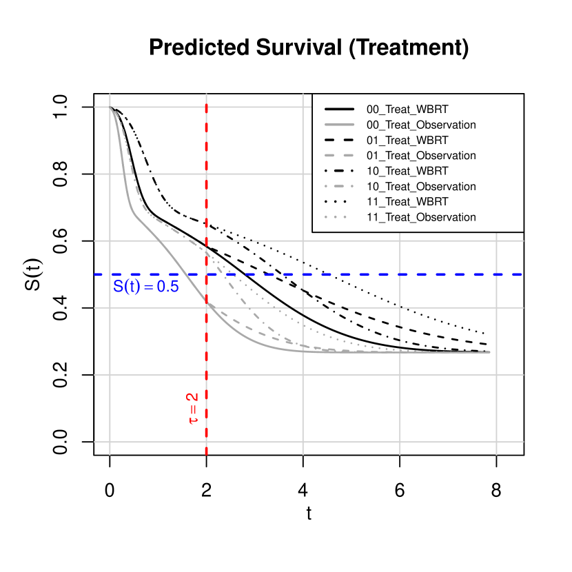
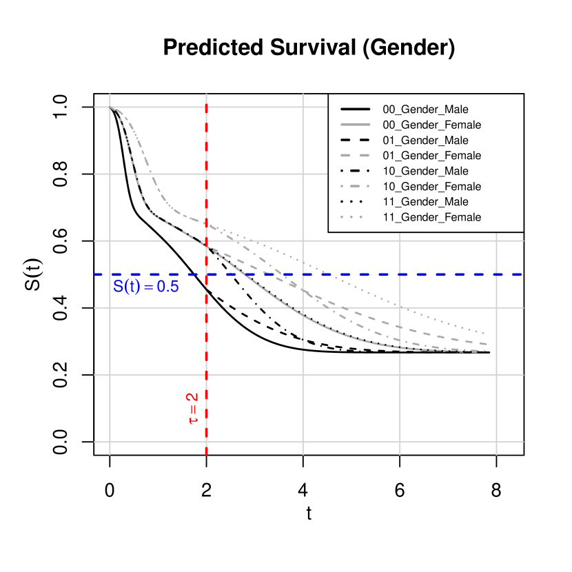
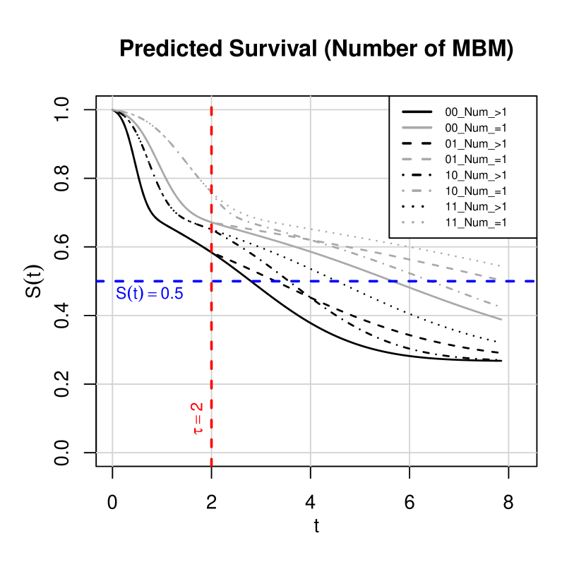
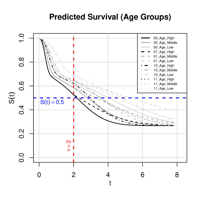
Figure 6: Figures of predicted survival curves (in years) for the five time-fixed covariates, treatment: WBRT (black lines) vs observation (dark grey lines), gender: male (black lines) vs female (dark grey lines), number of MBM: $>1$ (black lines) vs $=1$ (dark grey lines) and age: high (black lines) vs middle (dark grey lines) vs low (light grey lines), based on the four trajectories (line types) of the time-varying covariate, use of systemic therapy.

References

- Buckley and James, (1979) Buckley, J. and James, I. (1979). Linear regression with censored data. Biometrika, 66(3):429–436.
- Cai and Betensky, (2003) Cai, T. and Betensky, R. A. (2003). Hazard regression for interval-censored data with penalized spline. Biometrics, 59(3):570–579.
- Chan and Ma, (2012) Chan, R. H. and Ma, J. (2012). A multiplicative iterative algorithm for box-constrained penalized likelihood image restoration. IEEE Trans. Image Processing, 21:3168–3181.
- Chiou et al., (2014) Chiou, S. H., Kang, S., and Yan, J. (2014). Fitting accelerated failure time models in routine survival analysis with r package aftgee. Journal of Statistical Software, 61(11):1–23.
- Cox, (1972) Cox, D. R. (1972). Regression models and life-tables. Journal of the Royal Statistical Society: Series B, 34:187–202.
- Cox and Oakes, (1987) Cox, D. R. and Oakes, D. (1987). Analysis of Survival Data. Chapman and Hall, London.
- Eubank, (1999) Eubank, R. L. (1999). Nonparametric regression and spline smoothing. CRC press.
- Gao et al., (2017) Gao, F., Zeng, D., and Lin, D.-Y. (2017). Semiparametric estimation of the accelerated failure time model with partly interval-censored data. Biometrics, 73:1161–1168.
- Geman and Hwang, (1982) Geman, S. and Hwang, C.-R. (1982). Nonparametric maximum likelihood estimation by the method of sieves. The Annals of Statistics, 10(2):401–414.
- Hong et al., (2019) Hong, A., Fogarty, G., Dolven-Jacobsen, K., Burmeister, B., Lo, S., Haydu, L., Vardy, J., Nowak, A., Dhillon, H., Ahmed, T., Shivalingam, B., Long, G., Menzies, A., Hruby, G., Drummond, K., Mandel, C., Middleton, M., Reisse, C., Paton, E., and Thompson, J. (2019). Adjuvant whole-brain radiation therapy compared with observation after local treatment of melanoma brain metastases: A multicenter, randomized phase iii trial. Journal of Clinical Oncology, 37(33).
- Jin et al., (2003) Jin, Z., Lin, D., Wei, L., and Ying, Z. (2003). Rank-based inference for the accelerated failure time model. Biometrika, 90(2):341–353.
- Jin et al., (2006) Jin, Z., Lin, D. Y., and Ying, Z. (2006). On least-squares regression with censored data. Biometrika, 93(1):147–161.
- Kim, (2003) Kim, J. S. (2003). Maximum likelihood estimation for the proportional hazard model with partly interval-censored data. JRSSB, 65:489–502.
- Komárek et al., (2005) Komárek, A., Lesaffre, E., and Hilton, J. F. (2005). Accelerated failure time model for arbitrarily censored data with smoothed error distribution. Journal of Computational and Graphical Statistics, 14(3):726–745.
- Li and Ma, (2020) Li, J. and Ma, J. (2020). On hazard-based penalized likelihood estimation of accelerated failure time model with partly interval censoring. Stat Methods Med Res, 29(12):3804–3817.
- Lo et al., (2019) Lo, S. N., Hong, A., Haydu, L. E., Ahmed, T., Paton, E. J., Steel, V., Hruby, G., Tran, A., Morton, R. L., K, N. A., Vardy, J. L., Drummond, K. a. J., Dhillon, H. M., Mandel, C., Scolyer, R. A., R, M. M., Burmeister, B. H., Thompson, J. F., and B, F. G. (2019). Whole brain radiotherapy (wbrt) after local treatment of brain metastases in melanoma patients: Statistical analysis plan. Trials, 20(1):477.
- Ma, (2024) Ma, D. (2024). Semiparametric accelerated failure time model estimation with time-varying covariates. PhD thesis, Macquarie University.
- Ma et al., (2023) Ma, D., Ma, J., and Graham, P. L. (2023). On semiparametric accelerated failure time models with time-varying covariates: A maximum penalised likelihood estimation. Statistics in Medicine, 42(30):5577–5595.
- Ma et al., (2021) Ma, J., Couturier, D.-L., Heritier, S., and Marschner, I. (2021). Penalized likelihood estimation of the proportional hazards model for survival data with interval censoring. Int J Biostat, 18(2):553–575.
- Moore et al., (2008) Moore, T. J., Sadler, B. M., and Kozick, R. J. (2008). Maximum-likelihood estimation, the cramÉr–rao bound, and the method of scoring with parameter constraints. IEEE Transactions on Signal Processing, 56(3):895–908.
- Pan, (2000) Pan, W. (2000). A multiple imputation approach to Cox regression with interval-censored data. Biometrics, 56:199–203.
- Prentice, (1978) Prentice, R. L. (1978). Linear rank tests with right censored data. Biometrika, 65(1):167–179.
- Sun, (2006) Sun, J. (2006). The statistical analysis of interval-censored failure time data. Springer.
- Webb and Ma, (2023) Webb, A. and Ma, J. (2023). Cox models with time-varying covariates and partly-interval censoring–a maximum penalised likelihood approach. Statistics in Medicine, 42(6):815–833.
- Zeng and Lin, (2007) Zeng, D. and Lin, D. Y. (2007). Efficient estimation for the accelerated failure time model. Journal of the American Statistical Association, 102:1387–1396.