††thanks: * These authors contributed equally to this work.
Exact Thermal Eigenstates of Nonintegrable Spin Chains at Infinite Temperature
Yuuya Chiba*,chiba@as.c.u-tokyo.ac.jpDepartment of Basic Science, The University of Tokyo, 3-8-1 Komaba, Meguro, Tokyo 153-8902, Japan
Yasushi Yoneta*,yasushi.yoneta@riken.jpCenter for Quantum Computing, RIKEN, 2-1 Hirosawa, Wako, Saitama 351-0198, Japan
Abstract
The eigenstate thermalization hypothesis (ETH) plays a major role in explaining thermalization of isolated quantum many-body systems. However, there has been no proof of the ETH in realistic systems due to the difficulty in the theoretical treatment of thermal energy eigenstates of nonintegrable systems. Here, we write down analytically, for the first time, thermal eigenstates of nonintegrable spin chains. We consider a class of theoretically tractable volume-law states, which we call entangled antipodal pair (EAP) states. These states are thermal, in the most strict sense that they are indistinguishable from the Gibbs state with respect to all local observables, with infinite temperature. We then identify Hamiltonians having the EAP state as an eigenstate and rigorously show that some of these Hamiltonians are nonintegrable. Furthermore, a thermal pure state at an arbitrary temperature is obtained by the imaginary time evolution of an EAP state. Our results offer a potential avenue for providing a provable example of the ETH.
Introduction.—
Understanding the mechanism of thermalization in quantum many-body systems has been a pivotal issue in statistical physics [1, 2, 3]. Notably, the eigenstate thermalization hypothesis (ETH) [4, 5, 6] has served as a cornerstone in this field. It posits that all the energy eigenstates of quantum many-body systems exhibit thermal properties, thereby giving a plausible explanation of thermalization.
While the ETH is anticipated to hold in most nonintegrable systems, the verification of whether this hypothesis holds in realistic many-body systems relies on numerical calculations, and a theoretical verification has remained elusive [7, 8, 9, 10]. Thus, a significant challenge lies in theoretically addressing the nature of energy eigenstates, particularly in nonintegrable systems. However, it has not been clear whether thermal eigenstates of nonintegrable systems can be treated theoretically. This stems from the difficulty of writing down quantum states whose entanglement entropy obeys a volume law.
One approach to treat quantum many-body states theoretically is to use variational wave functions. Particularly for states that contain a small amount of entanglement, they can be represented via tensor network states such as a matrix product state (MPS) [11, 12]. Tensor network states are highly tractable, making them not only practical but also significantly contributing to theoretical advancements. Indeed, by utilizing the MPS, it has been successful to exactly describe finite-energy-density low-entangled (thus nonthermal) eigenstates even for nonintegrable systems [13, 14, 15], which are examples of many-body scars [16, 17, 18, 19, 20]. However, there has been a lack of variational wave functions suitable for theoretical analysis of volume-law states, which is one of the reasons why thermal eigenstates have not yet been obtained. Hence, there is a craving for a class of volume-law states amenable to the theoretical treatment [21, 22, 23, 24, 25].
In this Letter, we provide, for the first time, pairs of a nonintegrable Hamiltonian and its thermal eigenstate at infinite temperature.
We consider a class of volume-law states, which we call the entangled antipodal pair (EAP) states, that are amenable to theoretical calculations.
Then we fully characterize Hamiltonians having the EAP state as an eigenstate.
It is rigorously shown that some of these Hamiltonians are nonintegrable.
In addition, by evolving an EAP state in imaginary time, we construct a thermal pure state at arbitrary temperature, which is locally indistinguishable from the Gibbs state.
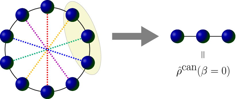
Figure 1: Schematic diagram depicting an entangled antipodal pair state . The antipodal pairs of spins linked by dotted lines are in the Bell states . For any subsystem with diameter smaller than or equal to half of the size of the entire system , the reduced density matrix coincides with the maximally mixed state, i.e., the Gibbs state at the inverse temperature .
Entangled antipodal pair state.—
We consider quantum spin- systems on the one-dimensional lattice with periodic boundary conditions. We assume that the number of lattice sites is even. Let be the Pauli matrices acting on the -th site, and and be the eigenvectors of .
Our goal is to obtain pairs of a nonintegrable Hamiltonian and its thermal eigenstate. To achieve this, we adopt the following strategy. First, we introduce a class of volume-law states that are theoretically tractable. Next, for each of these volume law states, we search for Hamiltonians that have it as a thermal eigenstate. Finally, we prove that some of these Hamiltonians are nonintegrable.
Following this strategy, as the first step, we introduce the entangled antipodal pair (EAP) state as 111Some special EAP states appear in the study of integrable systems [38, 39, 40].
(1)
Here are the Bell states between sites and defined by
(2)
where represents the negation of .
It is straightforward to check that
(3)
where , , and . Hence, the EAP state is uniquely characterized by and .
As a consequence of Eq. (3), the action of on the EAP state is equivalent to the action of , except for the factor of , i.e.,
(4)
This plays a key role in the proof of our main results.
Characteristically, the reduced density matrix of the EAP state for any subsystem with diameter of or less equals the maximally mixed state . Therefore, since the maximally mixed state coincides with the Gibbs state at the inverse temperature , it follows that the EAP state cannot be distinguished from the thermal equilibrium state at by any local measurement. Moreover, this implies that the bipartite entanglement between the subsystem consisting of contiguous spins and its complement is maximal. That is, the entanglement entropy of the EAP state obeys a volume low, with a coefficient reaching the maximum value .
This should be contrasted with the rainbow state [21, 22, 23, 24], which is a product of the Bell states between sites and . For a subsystem , the entanglement entropy of the rainbow state is and follows a volume law. However, for a subsystem , it strictly equals and follows an area law. As can be seen from this, the rainbow state is an athermal state that can be distinguished from the Gibbs state with an appropriate local observable.
EAP state as an energy eigenstate.—
As explained above, in the following, we search for Hamiltonians that have the EAP state as a thermal eigenstate. To this end, we consider the most general form of the Hamiltonian written as
(5)
In the first sum, represents a subset of . In the second sum, represents a combination of for . Here the origin of the energy is taken such that is traceless. Now we impose a very mild condition on the locality of interactions: for any subset with . (For instance, a nearest neighbor interacting system, where for , obviously satisfies the above condition for large .)
We are interested in the Hamiltonian where some EAP state is an energy eigenstate. Such Hamiltonians can be completely characterized by the following theorem 222See Supplemental Material for proofs of theorems, additional numerical results, and discussions..:
Theorem 1.
The following three statements are equivalent:
(i)
An EAP state is an eigenstate of .
(ii)
An EAP state is an eigenstate of with the eigenvalue .
(iii)
For all and ,
(6)
where and for .
Note that Eq. (6) has many solutions. In fact, for any given EAP state, one can construct many trivial Hamiltonians that consist of only a few local terms, e.g., with and satisfying Eq. (6). However, in most cases, such trivial Hamiltonians will be outside the scope of statistical mechanics. Therefore, in the following, we focus on cases where the Hamiltonian is translation invariant and show that only several EAP states are allowed as solutions of Eq. (6).
Translation-invariant nonintegrable Hamiltonians.—
Let us consider translation-invariant Hamiltonians with nearest neighbor interactions. They can include only interaction terms, , and magnetic field terms, . Solving Eq. (6) in Theorem 1, we can find all solutions of , and [27].
Interestingly, there are some nontrivial solutions whose are not invariant by single-site shift but invariant by -site shift for . To express such solutions efficiently, we introduce the following notation for EAP states that are invariant by -site shift 333Note that, for some of states (7), -site shift can cause a phase change, such as , where is the one-site translation operator.:
When is a multiple of ,
(7)
denotes the EAP state characterized by satisfying and for and .
For example, when is even, .
Using this notation, we can list all nontrivial solutions as follows:
Theorem 2.
By excluding noninteracting Hamiltonians 444There are only two solutions whose Hamiltonians are noninteracting [27]., the solution of Eq. (6) whose Hamiltonian is translation invariant and includes only nearest neighbor interactions and magnetic fields is restricted to the following:
1.
The EAP state is an eigenstate of
(8)
for arbitrary values of .
2.
When is a multiple of three, the EAP state is an eigenstate of
(9)
for arbitrary values of .
3.
When is a multiple of four,
the EAP state is an eigenstate of
(10)
for arbitrary values of .
and their equivalents obtained by appropriate permutations of directions of the Pauli matrices.
As shown in this theorem, there exist not so many solutions in the case of translation-invariant Hamiltonians, and this implies that our condition Eq. (6) is strong enough. Considering the importance of these models, we call the models described by , and Models 1, 2 and 3, respectively. Note that, since Model 2 is included in Model 1, the EAP state is also an eigenstate of .
Furthermore, we can obtain the following theorem regarding the nonintegrability of Models 2 and 3 [27]:
Theorem 3.
For Model 2 with and for Model 3 with , there exists no local conserved quantity other than a linear combination of the identity and the Hamiltonian (i.e., trivial one).
Because it is known that integrable systems have many [ number of] nontrivial local conserved quantities [30, 31, 32], the above theorem implies that these models are indeed nonintegrable.
In addition, since Model 2 (which is case of Model 1) is nonintegrable for any nonzero , Model 1 will be nonintegrable, at least for nonaccidental values of the parameters [27].
Combining Theorems 2 and 3 with the fact that EAP states are thermal as explained above, we first obtain, to our knowledge, an analytic expression of a thermal energy eigenstate of a nonintegrable system.
This highly contrasts with the recent progress made by H. Tasaki [33] in attempts to prove the ETH. He proved, only with respect to special observables, that all energy eigenstates of a certain noninteracting (integrable) system are indistinguishable from the thermal state. However, problems in nonintegrable systems remained elusive in his work. In addition, the restriction on observables is essential in his result because the integrable system has many local observables by which energy eigenstates can be distinguished from the thermal state. By contrast, our approach is to construct, in a nonintegrable system, an energy eigenstate that is indistinguishable from a thermal state with respect to any local observables.
Finite-temperature state.—
So far, we have only considered states at . Can we describe thermal states at using the EAP state? Here, we provide a method for constructing finite-temperature states using the EAP state. It should be noted that Hamiltonians considered here are not restricted to those having the EAP state as an eigenstate, which we have considered thus far.
Consider a system with translationally invariant short-range interactions. Suppose that is a real matrix with respect to the products of eigenstates of , . This class includes many well studied models in statistical mechanics, such as the Ising model and the Heisenberg model.
Here, we utilize the EAP state characterized by , i.e., in the notation introduced in Eq. (7). Then, as will be discussed below, the imaginary time evolution of the EAP state
(11)
is locally indistinguishable from the Gibbs state at the inverse temperature with an exponentially small error, although it is not an eigenstate of 555Some readers may wonder, if the EAP state is an energy eigenstate, then it is invariant under the imaginary time evolution, and hence cannot describe a finite temperature state. However, by using Theorem 1, it immediately follows that cannot be an energy eigenstate provided that is translation invariant (for single-site translations) and is a real matrix..
Let be a local observable of interest. Since both and are translation invariant, without loss of generality, we can assume that has support around . We then introduce an approximation for as
(12)
Here represents the interaction between the left half and the right half of the whole system, defined as a sum of interaction terms when is decomposed into a linear combination of the Pauli strings as in Eq. (5).
The imaginary time evolution is expected to be stable against local perturbations. Indeed, the Gibbs state, which is proportional to the imaginary time evolution operator, is not affected by perturbations on infinitely distant points because systems under consideration are one dimensional and do not exhibit the first-order phase transition [27]. Therefore, since is a sum of local observables defined around or at a distance of from the support of , it is expected that approximate around in the limit of , i.e.,
(13)
Under this assumption, we have the following [27]:
Theorem 4.
Suppose that is short ranged and translation invariant and is a real matrix in the basis formed by products of and . Let be an arbitrary local observable. Then, if Eq. (13) is satisfied, it holds that
(14)
In other words, is a thermal pure state at finite temperature while it is not an energy eigenstate. This is true for various systems where the Hamiltonian is a real matrix in the spin basis.
We finally confirm the validity of Eq. (14) by numerically testing our prediction on the transverse field Ising chain, defined by the Hamiltonian
(15)
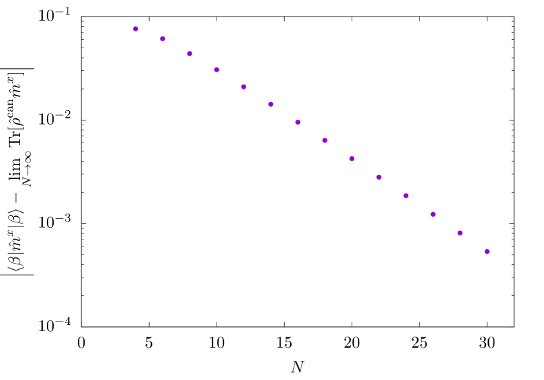
We plot in Fig. 2 the dependence of the difference in the expectation value of the transverse magnetization between the Gibbs state in the thermodynamic limit and the imaginary time evolved EAP state . We can confirm that the expectation value in converges to the correct value. Furthermore, the convergence is exponentially fast. Thus, by utilizing the EAP state evolved in imaginary time, one can calculate the thermal equilibrium values of local observables.
Here we discuss the relation with the cTPQ state [35], which is also a type of thermal pure states. The cTPQ state is the imaginary time evolution of a Haar random state. The Haar random state is (almost) maximally entangled and is locally indistinguishable from the maximally mixed state, as is the EAP state. However, while constructing the TPQ state requires an imaginary time evolution for , constructing requires only half of that, .
In addition, unlike the cTPQ state, does not entail statistical uncertainties. This means that generating a single suffices, without incurring any sampling costs.
Figure 2: dependence of the difference in the expectation value of the transverse magnetization between the Gibbs state in the thermodynamic limit and the imaginary time evolved EAP state for the transverse field Ising model. We set the transverse field to and the inverse temperature to .
Discussion.—
We have studied a class of volume-law states, which we call entangled antipodal pair (EAP) states, and thoroughly characterized these states by providing the necessary and sufficient conditions that Hamiltonians must satisfy in order to have an EAP state as an eigenstate. Moreover, we have rigorously shown that some of such Hamiltonians are nonintegrable. Our EAP states are indistinguishable from the Gibbs state at infinite temperature. In other words, we have written down, for the first time, analytic expressions for thermal energy eigenstates of nonintegrable many-body systems. We have also devised a method for constructing finite-temperature thermal states using an EAP state.
Some readers may be concerned that the energy eigenspace containing the EAP state is excessively large because, with an exponentially large number of states, it can be not so difficult to obtain a highly entangled state as their linear combination, even when each is hardly entangled.
However, numerical results show that in Model 1, the degeneracy of the EAP state is only two in the momentum sector 666Furthermore, by extending the locality of interactions from two to three, we have also obtained an example of a pair of the EAP eigenstate and the nonintegrable Hamiltonian that does not have degeneracy in the corresponding momentum sector [27].
In addition, we can also confirm that all states in the degenerate eigenspace obey a volume law with the maximal coefficient . Hence, the nontriviality of our findings is not diminished by the degeneracy.
Our result suggests that theoretical analysis may be feasible even for thermal eigenstates of nonintegrable systems and may pave the way for giving a provable example of the ETH. Since EAP states themselves are at infinite temperature, constructing finite temperature thermal eigenstates remains challenging. However, as we have shown, one can obtain thermal states at arbitrary temperature by applying an imaginary time evolution, a low-complexity operation that can be well approximated via a matrix product operator with small bond dimension [37], to the EAP state. This implies that the expressivity of states derived from EAP states is quite high. Thus, EAP states would be one of the most promising starting points for constructing thermal eigenstates at finite temperature.
Furthermore, it will provide theoretical methodologies not only for thermalization, but also for various areas of quantum statistical mechanics that use thermal pure states, such as the formulation of statistical mechanics and finite temperature simulations.
Acknowledgement.—
We are grateful to N. Shiraishi, A. Shimizu, H. Katsura, K. Fujii, K. Mizuta, H. Kono, M. Yamaguchi, and Z. Wei for useful discussions.
We would like to especially thank H. K. Park for careful reading and valuable comments on a draft of this paper.
YY is supported by the Special Postdoctoral Researchers Program at RIKEN. YC is supperted by Japan Society for the Promotion of Science KAKENHI Grant No. JP21J14313.
Note added:
After the completion of this work, we became aware of a recent related work by A. N. Ivanov and O. I. Motrunich (arXiv:2403.05515) which constructs an exact volume-law eigenstate of the PXP and related models.
References
D’Alessio et al. [2016]L. D’Alessio, Y. Kafri, A. Polkovnikov, and M. Rigol, Adv. Phys. 65, 239 (2016).
Bernien et al. [2017]H. Bernien, S. Schwartz, A. Keesling, H. Levine, A. Omran, H. Pichler, S. Choi, A. S. Zibrov, M. Endres, M. Greiner, V. Vuletic, and M. D. Lukin, Nature (London) 551, 579 (2017).
Turner et al. [2018a]C. J. Turner, A. A. Michailidis, D. A. Abanin, M. Serbyn, and Z. Papić, Nat. Phys. 14, 745 (2018a).
Turner et al. [2018b]C. J. Turner, A. A. Michailidis, D. A. Abanin, M. Serbyn, and Z. Papić, Phys. Rev. B 94, 155134 (2018b).
Note [5]Some readers may wonder, if the EAP state is an energy eigenstate, then it is invariant under the imaginary time evolution, and hence cannot describe a finite temperature state. However, by using Theorem 1, it immediately follows that cannot be an energy eigenstate provided that is translation invariant (for single-site translations) and is a real matrix.
Note [6]Furthermore, by extending the locality of interactions from two to three, we have also obtained an example of a pair of the EAP eigenstate and the nonintegrable Hamiltonian that does not have degeneracy in the corresponding momentum sector [27].
Note [9]The results of exact diagonalization also show that, at least for , degeneracy at in the whole Hilbert space remains only two. This means that all eigenstates of the Hamiltonian (S221) with eigenenergy are given by (linear combinations of) the EAP states .
Supplemental Material for
“Exact Thermal Eigenstates of Nonintegrable Spin Chains at Infinite Temperature”
For the proof of Theorem 1, the following lemma is crucial:
Lemma 1.
Let and be subsets of satisfying and . For any EAP state , we have
(S1)
Proof.
We divide the lattice into four equally sized parts, .
Since , without loss of generality, we can take .
Since , cannot have any intersection with both and ,
or with both and .
Suppose that and let .
Because no Pauli operator acts on its antipodal site in the left hand side of Eq. (S1), we have
(S2)
If , we can obtain the same result in almost the same manner.
Therefore, in the following, we only need to consider the two cases and .
Next we consider the case of .
In the left hand side of Eq. (S1), at most two Pauli operators act on each site , and no Pauli operator acts on its antipodal site .
Therefore, unless and for all ,
the left hand side of Eq. (S1) becomes zero.
On the other hand, if and for all , we obviously have
(S3)
Finally we consider the case of .
In the left hand side of Eq. (S1), at most one Pauli operator acts on each site , and at most one Pauli operator acts on its antipodal site .
Using Eq. (4) of the main text, we have
(S4)
Applying the arguments of the previous paragraph, we can obtain the following: Unless and for all ,
the left hand side of Eq. (S1) becomes zero.
On the other hand, if and for all , we have
which is equivalent to statement (ii). It obviously implies statement (i).
∎
Remark: The above proof also shows that, if we only need to show (iii) (ii), we can relax the condition on the locality of interactions in the main text, “ for any subset with ” to “ for any subset with .”
II List of translation-invariant and nearest-neighbor-interacting Hamiltonians
We provide a list of translation-invariant (for single-site translations) and nearest-neighbor-interacting Hamiltonians having an EAP state as an eigenstate. First, we exclude the case of free spins, as it is trivial. Next, for some cases where only one of is non-zero, we find that EAP states are degenerate, so we also exclude such cases. Then pairs of the EAP state and the Hamiltonian are limited to the following five types (and their equivalents obtained by appropriate permutations of directions of the Pauli matrices). It can be readily confirmed through direct calculations that the pairs of the EAP state and the Hamiltonian listed below satisfy Eq. (6).
II.1 Case where the EAP state is invariant under -site translation
The EAP state is an eigenstate of the Hamiltonian defined by
(S14)
for arbitrary values of .
This model is Model 1 in Theorem 2.
II.2 Case where the EAP state is invariant under -site translation
Suppose that is a multiple of two.
The EAP state is an eigenstate of the Hamiltonian defined by
(S15)
for arbitrary values of .
This model can be mapped onto free fermions via the Jordan-Wigner transformation.
In addition, the EAP state is an eigenstate of the Hamiltonian defined by
(S16)
for arbitrary values of .
This model can also be mapped onto free fermions via the Jordan-Wigner transformation.
II.3 Case where the EAP state is invariant under -site translation
Suppose that is a multiple of three.
The EAP state is an eigenstate of the Hamiltonian defined by
(S17)
for arbitrary values of .
This model is Model 2 in Theorem 2. As shown in Theorem 3, this model is nonintegrable.
II.4 Case where the EAP state is invariant under -site translation
Suppose that is a multiple of four.
The EAP state is an eigenstate of the Hamiltonian defined by
(S18)
for arbitrary values of .
This model is Model 3 in Theorem 2. As shown in Theorem 3, this model is nonintegrable.
First we define a -local conserved quantity (which is the same as one given in Ref. [41]) by the operator that commutes with the Hamiltonian
(S19)
and can be written as
(S20)
Here represents a sequence of symbols, satisfying
(S21)
(S22)
and represents the product of the corresponding Pauli operators on the sites :
(S23)
In Eq. (S20), are the expansion coefficients. [We add the superscript in order to emphasize its value.] The crucial point of Eq. (S20) is that does not include with .
Now we give the precise expression of Theorem 3 of the main text, which is represented by the following two theorems:
Theorem 3.A.
In Model 2 with , and for ,
there is no -local conserved quantity that is linearly independent of the Hamiltonian and the identity.
Theorem 3.B.
In Model 3 with , and for ,
there is no -local conserved quantity that is linearly independent of the Hamiltonian and the identity.
In the remaining of this section, we prove these theorems by adapting the theoretical approach to prove the absence of local conserved quantities, which was introduced by N. Shiraishi [42]. There are only a few examples of such proofs [42, 41, 43]. This approach starts from solving Eq. (S19) with respect to the coefficients with largest locality, , and showing that . When solving Eq. (S19), we need to calculate many commutators such as
(S24)
(S25)
For simplicity of notation, we write in place of . In order to express such calculations efficiently, we use the following diagrammatic notation:
(S38)
These four diagrams correspond to the four terms in Eq. (S25). In each diagram, the first row represents the term from , the second row the term from , and the third row the result of the commutator.
For simplicity of notation, we add the site index only for the leftmost operators in the third row. In addition, we call the first row of the diagram “-local input”, and the third row of the diagram “-local output”, when they consist of , , , and on consecutive sites.
This subsection proves Theorem 3.A.
Throughout this subsection, we consider Model 2 and assume and .
(The reason for the assumption is the same as one discussed in Sec. VI A of Ref. [41].)
Proof.
The proof of Theorem 3.A is divided into three parts.
The first part investigates the coefficients with largest locality, . For the coefficients of the form , we have
(S42)
Because a -local output can be obtained only when the Hamiltonian term is applied to the edges of -local inputs, there are at most two -local inputs that contribute to one -local output.
However, since the left end of the output of Eq. (S42) is , the other contribution does not exist.
Furthermore, from Eq. (S19), the sum of all contribution to the output must vanish, and therefore we have
(S43)
In a similar manner, we can obtain the following lemma:
for all .
Here the symbols that are not specified can be any symbols satisfying Eqs. (S21) and (S22).
Furthermore, we can obtain relation between two of the remaining -local inputs as in
(S64)
which results in
(S65)
If is not , we have from Lemma 3, and hence .
By using such a relation, we can shift the symbols to the left and we can determine these symbols.
As a result, we can obtain the following proposition:
Proposition 1.
For any and for any , the solution of Eq. (S19) satisfies
(S66)
except for
(S67)
In addition, these remaining coefficients are independent of the site and satisfy
(S68)
Here we used a shorthand notation of a sequence of symbols
(S69)
Therefore we only need to show that one of these remaining coefficients is zero.
As the second part of the proof, we examine the coefficient .
We consider the contribution from to a -local output which can also include the contribution from -local inputs.
For instance,
(S76)
are the only contribution to the -local output , and hence we have
(S77)
For coefficients of -local inputs, we obtain the following:
All contributions to -local output (for ) are given by
(S84)
(S91)
which result in
(S92)
For the coefficient , which appears in case of the above equation, we can obtain another relation
(S93)
in a similar manner.
We can also obtain the following relation for the coefficient ,
(S94)
by considering the contributions to ,
(S107)
Because the sum of the left-hand sides of Eqs. (S77), (S92)–(S94) (by choosing the site appropriately) become zero, we have
This means that is a -local conserved quantity.
Applying the same argument to , ,…, and -local conserved quantity, we can show that any -local conserved quantity with have to be a -local conserved quantity.
As the third part of the proof, we analyze the coefficients with in the case of .
From Lemma 2, we only need to consider the coefficients of the form and .
Furthermore, the coefficient vanishes because
(S115)
is the only contribution to the -local output .
The coefficient vanishes by a similar reason.
In addition, because -local output comes only from -local input,
we can easily show that .
For the remaining coefficients and , we can easily show that they are independent of the site and are related to each other by
(S116)
which results in the following proposition:
Proposition 3.
Any -local conserved quantity can be written as
(S117)
with arbitrary constants .
From Eq. (S111) and Proposition 3, we obtain Theorem 3.A.
∎
This subsection proves Theorem 3.B.
Throughout this subsection, we consider Model 3 and assume and .
(The reason for the assumption is the same as one discussed in Sec. VI A of Ref. [41].)
Proof.
The proof of Theorem 3.A is divided into three parts.
The first part investigates the coefficients with largest locality, .
In a manner similar to the proof of Lemma 2, we can show the following lemma:
for all .
Here the symbols that are not specified can be any symbols satisfying Eqs. (S21) and (S22).
By shifting the symbols to the left as we did to obtain Proposition 1, many coefficients can be shown to be zero.
To explain the result, we introduce a version of “doubling product.”
It was originally introduced by N. Shiraishi [42].
Our version is modified for analyzing Model 3 as follows:
We call a sequence of the Pauli operators doubling product, if it can by written as , where
(S124)
(S125)
Here is chosen from to make its coefficient .
In addition, we introduce by
(S126)
(S127)
Then we can obtain the following proposition:
Proposition 4.
For any and for any other than doubling product, the solution of Eq. (S19) satisfies
(S128)
For the case where is given by a doubling product Eqs. (S124) and (S125), these remaining coefficients are independent of the site and are related to each other by
(S129)
for any .
Therefore we only need to show that one of these remaining coefficients is zero.
As the second part of the proof, we examine the coefficient .
We consider the contribution from the -local input to a -local output which can also include the contribution from -local inputs. For instance,
(S142)
are the only contribution to the -local output .
Note that the contribution from the third diagram vanishes because of Lemma 4, and the contribution from the second diagram satisfies
(S143)
because can be written as a doubling product and Eq. (S129) in Proposition 4 is applicable.
Hence we have
(S144)
In a similar manner, we can obtain
(S145)
(S146)
(S147)
(S148)
from the diagrams
(S161)
(S174)
(S181)
(S188)
(S198)
respectively.
Because the sum of the left-hand sides of Eq. (S144) and of Eqs. (S145)–(S148) (by choosing the site appropriately) become zero, we have
This means that is a -local conserved quantity.
Applying the same argument to , ,…, and -local conserved quantity, we can show that any -local conserved quantity with have to be a -local conserved quantity.
As the third part of the proof, it is straightforward to show the following proposition:
Proposition 6.
Any -local conserved quantity can be written as
(S203)
with arbitrary constants .
From Eq. (S202) and Proposition 6, we obtain Theorem 3.B.
∎
In the paragraph below Theorem 3 of the main text, we explained that Model 1 is expected to be nonintegrable.
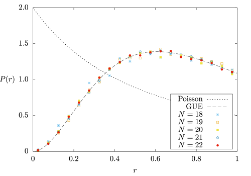
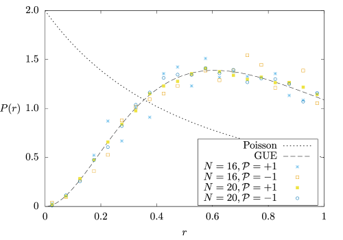
To confirm this expectation, we numerically investigate the level spacing statistics [44, 45] of Model 1 by exact diagonalization. Figure S1 plots the distribution of the ratio of consecutive level spacings [45]
(S204)
constructed from eigenenergy in the eigenspace of translation with momentum 777To remove the possibility of accidental discrete symmetries, we avoid eigenspace of special momentum such as and .
(sorted in descending order). We set the parameters as 888We can always take by an appropriate rotation around axis.. The plot is well described by the Gaussian unitary ensemble distribution [45] (dashed line) and well separated from the Poisson distribution [45] (dotted line). This shows that Model 1 (with above mentioned parameters) has no nontrivial local conserved quantity, implying nonintegrability of the model.
Figure S1: Distribution of the ratio of consecutive level spacings of Model 1 in Theorem 2 in the main text. We use eigenenergies in the subspace of momentum .
Let be a bit string of length . Then, using , we define the the computational basis as
(S205)
As a preparation, we clarify the properties of the Hamiltonian satisfying the assumptions of the theorem. Since Pauli strings form an orthogonal basis of operators on the whole Hilbert space, the Hamiltonian can be uniquely expressed as a linear combination of them:
(S206)
With this notation, in the main text is written as
(S207)
where and . Since, is translation invariant by assumption, we have
(S208)
Here, is the Hamiltonian for the same system of length , but with open boundary conditions rather than periodic boundary conditions:
(S209)
Under the complex conjugation with respect to the computational basis, the Pauli string behaves as
(S210)
where is the number of Pauli matrices along the -direction, , within the Pauli string. Thus, the complex conjugation transforms the Hamiltonian as
(S211)
Since the expansion in terms of Pauli strings is unique, for to be a real matrix in the computational basis (i.e., ), must be zero when is odd. Hence, we obtain
(S212)
Therefore, is also a real matrix in the computational basis.
We now proceed to prove Eq. (14). The EAP state can be expanded in the computational basis for subsystems and as
Since is a real matrix with respect to the computational basis, it holds that
(S215)
for any and .
Substituting this into Eq. (S214), we obtain
(S216)
Therefore, for any observable defined on the subsystem , we get
(S217)
where is the Gibbs state for . Hence the thermodynamic limit yields
(S218)
In the thermodynamic limit, the Gibbs state converges to the KMS state regardless of whether periodic or open boundary conditions are imposed. Since we are now considering a one-dimensional system, there exists a unique KMS state at finite temperature [48, 49]. Consequently, expectation values of local observables in the Gibbs state do not depend on boundary conditions in the thermodynamic limit. Thus, using Eq. (13), we finally obtain
According to Theorem 2, the EAP state is an energy eigenstate with an eigenvalue of Model 1 for arbitrary parameters. Without loss of generality, we can take by an appropriate rotation around axis, so we set the parameters of Model 1 as . By the exact diagonalization, we find that is doubly degenerate in the zero-momentum sector for . Let us investigate entanglement properties of states in this eigenspace, which we will write as . Let denote the state orthogonal to in . All states in can be expressed as a linear combination of and :
(S220)
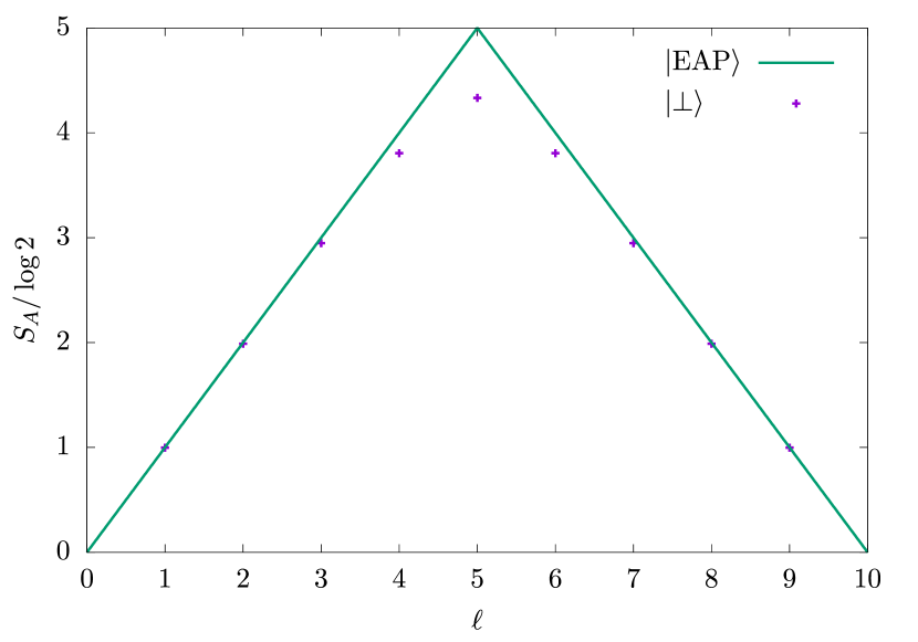
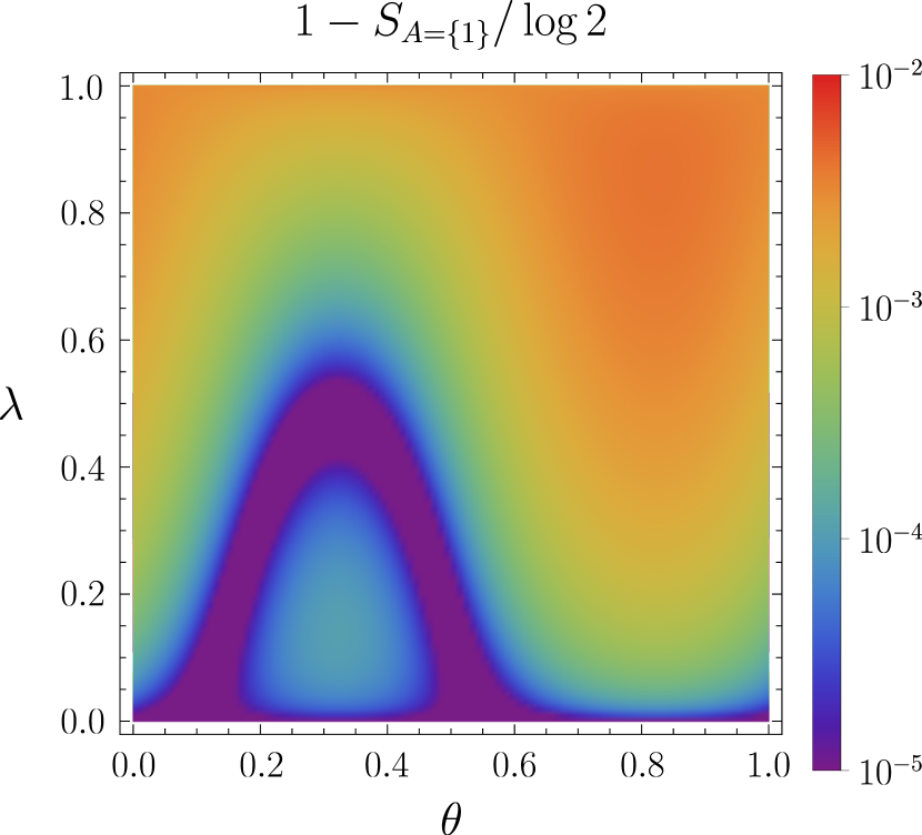
First, we investigate the bipartite entanglement in (corresponding to the case of ). We plot in Fig. S3 the entanglement entropy between a subsystem of length and its complement as a function of . It can be seen that is almost maximally entangled, but is different from EAP states.
Next, we confirm that all states in the eigenspace are maximally entangled states. To investigate the coefficient of the volume-law scaling, we compute the entanglement entropy of between a subsystem of length and its complement for various and and show in Fig. S3 the deviation from the coefficient of the maximally entangled state, . It can be observed that for all states in , the volume-law coefficients are significantly close to the maximal coefficient.
Thus, there are not any low entangled states in the eigenspace, and hence the EAP state is not a superposition of such states.
Figure S2: Entanglement entropy of the EAP state and its orthogonal degenerate state between a subsystem of length and its complement as a function of for Model 1 with . We set the parameters as .
Figure S3: Deviation of the volume-law coefficient of the entanglement entropy of zero-energy eigenstates defined by Eq. (S220) in the zero-momentum sector of Model 1 from that of the maximally entangled state. We set the parameters as and .
VI.2 Nondegenerate Hamiltonian with next-nearest-neighbor interactions
In this subsection, by extending the Hamiltonian (S16) to the next-nearest-neighbor interacting one, we provide a Hamiltonian having an EAP state as an eigenstate that is nondegenerate in the corresponding momentum sector.
Suppose that is translation invariant and satisfies for any subset with . Then, it can be characterized by coupling constants, , and ( and , where ). From Theorem 1 of the main text, it is straightforward to show that, when is a multiple of , the EAP states and are eigenstates of if and only if can be written as
(S221)
Here all parameters are arbitrary, and hence it is an extension of Eq. (S16).
Because the EAP states and are related to each other by translation as
(S222)
(S223)
their superposition is included in the eigenspace of translation with the momentum . Therefore, we investigate degeneracy of energy eigenvalues in the subspace of . We set , , , , , , , , , and . By exact diagonalization, we numerically find that, at least for , the eigenvalue is nondegenerate in the subspace of .
We also verify the nonintegrability of model (S221). Because of the existence of , model (S221) is not mapped to a free fermionic (integrable) system by the Jordan-Wigner transformation. We confirm nonintegrability of model (S221) by calculating the distribution of the ratio of consecutive level spacings, as in Fig. S1. Figure S4 plots the distribution constructed from energy eigenvalues in the eigenspace of translation and transformation with momentum and parity . This plot is well described by the Gaussian unitary ensemble distribution [45] (dashed line) and well separated from the Poisson distribution [45] (dotted line), indicating the nonintegrability of the model.
Figure S4: Distribution of the ratio of consecutive level spacings of model (S221). We use eigenenergies in the subspace of momentum and parity (regarding rotation by around -axis). The parameters are given below Eq. (S223).
Note that, because the interference term between and does not affect the expectation values of local observables whose support size are less than , any state described by a linear combination of and is locally indistinguishable from the maximally mixed state.
Combining all results of this subsection, we can say that the state is a thermal eigenstate of the nonintegrable Hamiltonian (S221), and is nondegenerate in the corresponding momentum sector 999The results of exact diagonalization also show that, at least for , degeneracy at in the whole Hilbert space remains only two. This means that all eigenstates of the Hamiltonian (S221) with eigenenergy are given by (linear combinations of) the EAP states ..