ALP contribution to the Strong CP problem

Abstract

We compute the one-loop contribution to the $\bar{\theta}$-parameter of an axion-like particle (ALP) with CP-odd derivative couplings. Its contribution to the neutron electric dipole moment is shown to be orders of magnitude larger than that stemming from the one-loop ALP contributions to the up- and down-quark electric and chromoelectric dipole moments. This strongly improves existing bounds on ALP-fermion CP-odd interactions, and also sets limits on previously unconstrained couplings. The case of a general singlet scalar is analyzed as well. In addition, we explore how the bounds are modified in the presence of a Peccei-Quinn symmetry.

I Introduction

Axion-like particles (ALPs) are singlet pseudo-Goldstone bosons (pGBs) that emerge as a consequence of the spontaneous breaking of a global symmetry. They are motivated by a variety of scenarios that aim to solve some of the shortcomings of the Standard Model of Particle Physics (SM). This includes scenarios which solve the strong CP problem Peccei:1977hh ; Peccei:1977ur ; Weinberg:1977ma ; Wilczek:1977pj , theories with extra space-time dimensions ArkaniHamed:1998pf ; Dienes:1999gw ; Chang:1999si ; DiLella:2000dn , some dynamical flavour theories Wilczek:1982rv ; Ema:2016ops ; Calibbi:2016hwq , dark matter models Abbott:1982af ; Dine:1982ah ; Preskill:1982cy , scenarios which explore a dynamical origin for Majorana neutrino masses Gelmini:1980re and string theory models Cicoli:2013ana , among others. Consequently, the study of ALPs is currently under intense investigation, marked by a surge in experimental proposals and robust theoretical endeavors. The most prominent among those pGB candidates is the QCD axion Peccei:1977hh ; Peccei:1977ur ; Weinberg:1977ma ; Wilczek:1977pj , which aims to explain the absence of CP violation in the strong sector by dynamically relaxing the $\bar{\theta}$-parameter to the CP conserving point.

Flavour preserving, low energy CP-odd observables are predicted by the SM to be very small, since they are suppressed by a combination of small quark masses and small CKM mixing angles, and first arise at multi-loop level in the perturbative expansion. Hence they are powerful probes of new sources of CP violation. Prime among these observables is the electric dipole moment (EDM) of the neutron (nEDM) which is estimated at $d_{n}\sim 10^{-34}\;e\cdot\text{cm}$ Khriplovich:1981vs ; Khriplovich:1981ca ; Khriplovich:1985jr , some seven orders of magnitude smaller than the current experimental bound Abel:2020pzs ; Pendlebury:2015lrz .

In this work, we focus on the case of a generic ALP (i.e. with shift-symmetric couplings to SM fermions). Inspired by the QCD axion, most of the effort in ALP phenomenology has been devoted to study the CP-conserving couplings of ALPs to SM particles. However, CP-violating ALP signatures are gaining increased interest DiLuzio:2020oah ; OHare:2020wah ; Dekens:2022gha ; DiLuzio:2023edk ; Plakkot:2023pui ; Bonnefoy:2022rik ; Grojean:2023tsd ; Bauer:2021mvw .

Indeed, derivative ALP-fermion interactions can have CP-odd couplings, and it turns out that they may contribute to quark electric dipole moments (qEDMs) at one loop. These and the resulting contribution to the nEDM have been computed elsewhere DiLuzio:2020oah . In this work, we compute instead the one-loop contribution to $\bar{\theta}$ of an ALP with CP-odd derivative couplings to the SM quarks. We will show that its contribution to the nEDM is parametrically distinct than that of quark electric dipole moments and can be numerically much more important. For completeness, the contribution to $\bar{\theta}$ of a generic scalar is also computed and compared.

Figure -1019: One loop corrections to the fermion masses.

II Set-up: Derivative fermionic ALP Lagrangian

Let us consider an ALP $a$, defined as a spin-0 field, singlet of the SM, and described by a Lagrangian invariant under the shift symmetry $a\rightarrow a+\textrm{constant}$, except for a small mass term $m_{a}\ll f_{a}$ where $f_{a}$ is the ALP physics scale. We focus here on effective ALP-fermion interactions up to $\mathcal{O}(1/f_{a})$ terms. At scales $\mu\lesssim f_{a}$, these purely derivative interactions are encoded in the following effective Lagrangian:

$$\mathcal{L}_{a}\supset\frac{1}{2}\partial_{\mu}a\partial^{\mu}a-\frac{1}{2}m_{a}^{2}a^{2}+\big{(}\bar{u}_{L}\bm{M}_{u}u_{R}+\bar{d}_{L}\bm{M}_{d}d_{R}+\text{h.c.}\big{)}\\ +\bar{\theta}_{0}\frac{\alpha_{s}}{8\pi}G_{\mu\nu}\widetilde{G}^{\mu\nu}+\frac{\partial_{\mu}a}{f_{a}}\big{(}\bar{u}_{L}\gamma^{\mu}\bm{C}_{Q}u_{L}+\bar{u}_{R}\gamma^{\mu}\bm{C}_{u_{R}}u_{R}\\ +\bar{d}_{L}\gamma^{\mu}\bm{C}_{Q}d_{L}+\bar{d}_{R}\gamma^{\mu}\bm{C}_{d_{R}}d_{R}\big{)},$$ (1)

where $m_{a}$ is the ALP mass, $\bm{C}_{Q,u_{R},d_{R}}$ are hermitian $3\times 3$ matrices in flavour space and $\bm{M}_{u,d}$ are the up-type and down-type quark $3\times 3$ mass matrices. Note that the ALP couplings to $u_{L}$ and to $d_{L}$ are identical as mandated by the SM electroweak $SU(2)\times U(1)$ gauge invariance. Because of the hermiticity of the ALP-fermion coefficient matrices, only the flavour off-diagonal ALP-fermion couplings can lead to observable effects of CP-violation. The SM fermion mass terms are also shown in Eq. (1) and taken to be real and diagonal, so that the overall phase of the argument of the determinant of the mass matrices is already included in the $\bar{\theta}$-term, where $\bar{\theta}_{0}\equiv\bar{\theta}(\mu=\mu_{0})\big{|}_{\rm tree}$ and $\mu_{0}\equiv f_{a}$.

Our objective in this work is to compute the leading contribution of the fermionic ALP couplings to $\bar{\theta}$ (and its subsequent impact on the nEDM), which arises at one loop, as we will see next; see Fig. -1019. We assume that the ALP mass is larger than the QCD scale, $m_{a}\gtrsim 1\,\text{GeV}$. Let us consider an effective field theory (EFT) below the scale $\mu_{2}=\text{min}(m_{t},m_{a})$. The parameters in this EFT are computed by matching at the scale $\mu=\mu_{2}$, and receive contributions from integrating out both the ALP and the top quark. Let us focus first on the contribution to the phase of the up quark mass. The details of the computation of the one-loop diagram in Fig. -1019 are given in the next section, but let us anticipate that the contribution to $\bar{\theta}$ will turn out to be dominated by the top loop, provided all entries of $\bm{C}_{Q,u_{R},d_{R}}$ are of the same order, and reads

$$\Delta\bar{\theta}_{\rm ALP}\simeq\frac{m_{t}\,\text{max}(m_{a}^{2},m_{t}^{2})}{16\pi^{2}f_{a}^{2}m_{u}}\text{Im}(\bm{C}_{Q}^{13}\bm{C}_{u_{R}}^{*13})\,.$$ (2)

The dependence of this formula on the top mass is highly relevant, e.g. for $m_{a}<m_{t}$ it is cubic, a behaviour that will be transmitted to the ensuing contribution to the nEDM. This $\bar{\theta}$-induced contribution to the nEDM will be shown to be several orders of magnitude larger than that obtained in Ref. DiLuzio:2020oah through the contribution to the quark EDMs, as the latter only depends on $m_{t}$ linearly.

The mass dependence in Eq. 2 can be readily understood using the chirality-flip basis (described in App. A) instead of the derivative basis in Eq. 1. In the chirality-flip basis, there are two relevant Feynman diagrams to be considered, shown in Fig. -1016. In order for the upper diagram in Fig. -1016 with an internal top quark to contribute to the $\bar{u}_{L}u_{R}$ term, a mass insertion $\propto m_{t}$ inside the loop provides the required chirality flip. Each vertex contributes a factor of $m_{t}/f_{a}$. Since the loop depends on the renormalization scale only logarithmically the diagram gives a contribution that scales with $m_{t}$ and $f_{a}$ as $m_{t}^{3}/f_{a}^{2}$. The loop in the second diagram in Fig. -1016 is quadratic in $m_{a}$ and the vertex contributes a factor of $m_{t}/f_{a}^{2}$. So the contributions of the first and second diagram scale as $m_{t}^{3}/f_{a}^{2}$ and $m_{t}m_{a}^{2}/f_{a}^{2}$, respectively, and both contain a factor of $\bm{C}_{Q}^{13}\bm{C}_{u_{R}}^{*13}$. Finally, since we are computing the contribution to the phase of the up quark mass term, the result is inversely proportional to the absolute value of the quark mass itself, explaining the $1/m_{u}$ factor in Eq. 2 (see footnote 2).

The result can also be understood in the derivative basis in Eq. 1, in which only the diagram in Fig. -1019 contributes, but rather than obtaining the factors of $m_{t}^{2}$ and $m_{a}^{2}$ from the vertices, they arise from the quadratically divergent loop integral. We have verified that both bases give the same results for the explicit computations presented in Sec. III.

It is easy to see as well that the contributions to other CP-violation observables do not scale as $m_{t}\text{max}(m_{t}^{2},m_{a}^{2})$. Take for example the contribution to the quark EDM, $d_{q}$, and use again the chirality-flip basis of the Lagrangian. At one-loop it arises exclusively from the diagram in Fig. -1017; there is no contribution from the analogue of that for the up quark mass from the bottom diagram in Fig. -1016 because the photon cannot couple to the neutral axion. The chirality flip and the vertices give a factor of $m_{t}^{3}/f_{a}^{2}$, but now dimensional analysis dictates that the loop integral gives an additional factor of $1/m_{t}^{2}$, so that $d_{q}\sim m_{t}/f_{a}^{2}$.

The Lagrangian in Eq. 1 includes all operators that contribute at order ${\mathcal{O}}(1/f_{a}^{2})$ to $\Delta{\bar{\theta}}_{\rm ALP}$ in the derivative basis. There exist a single shift-symmetric operator with mass dimension 5 Georgi:1986df ; Brivio:2017ije ; Gavela:2019wzg and another one with dimension 6 Weinberg:2013kea ; Bauer:2022rwf , both involving the Higgs. They are not displayed in Eq. 1 since they are CP-even and thus do not contribute to $\Delta{\bar{\theta}}_{\rm ALP}$. Beyond these, there are CP-odd operators with mass dimension 7 and thus $\mathcal{O}(1/f_{a}^{3})$.

It is also worth noting that, since we are assuming $m_{a}\gtrsim 1\,\text{GeV}$, including the operator $aG\tilde{G}$ in the Lagrangian would not introduce a dynamical mechanism relaxing ${\bar{\theta}}$ to zero. That is, it would not amount to promoting the ALP to a QCD axion with a true PQ symmetry (that would require $m_{a}\to 0$).

III Computation of the contribution to $\bar{\theta}$

We perform in this section the one-loop matching of the Lagrangian in Eq. 1 to the following QCD Lagrangian:

$$\mathcal{L}_{\rm QCD,CPV}=\bar{\theta}\frac{\alpha_{s}}{8\pi}G_{\mu\nu}\widetilde{G}^{\mu\nu}+\sum_{q=u,d,s}\bar{q}\,m_{q}q\;-\\ -\frac{i}{2}\sum_{q=u,d,s}\left[d_{q}F_{\mu\nu}\;\bar{q}\sigma^{\mu\nu}\gamma_{5}q+g_{s}\,\tilde{d}_{q}\,G_{\mu\nu}\;\bar{q}\sigma^{\mu\nu}\gamma_{5}q\;\right]+\cdots$$ (3)

where $q=u,d,s$ denote the three lighter quark fields(up-, down- and strange-quarks), while $d_{u,d,s}$ and $\tilde{d}_{u,d,s}$ stand for their respective qEDMs and chromo-EDMs (cEDMs), and $F_{\mu\nu}$ and $G_{\mu\nu}$ denote the QED and QCD field strength tensors, respectively. Other dimension five operators (such as the Weinberg operator) are left implicit in the ellipsis.

The calculation of $\bar{\theta}$ proceeds in standard effective field theoretical fashion: starting from the EFT defined in Eq. 1, we run $\bar{\theta}$ from $\mu_{0}$ to $\mu_{1}\approx\text{max}(m_{t},m_{a})$, and then match $\theta$ to $\theta^{\prime}$ defined in EFT^′, a new effective theory where the heaviest of the top quark and the ALP has been integrated out. Then run $\bar{\theta}^{\prime}$ to $\mu_{2}$ where the lighter of the top quark and the ALP is integrated out and a new $\theta^{\prime\prime}$ for a new EFT^′′ is computed. This effective theory is QCD+QED with 5 flavours of quarks. To perform the calculation we find the renormalization group equation (RGE) in the EFT, use it to determine the functional form of $\bar{\theta}(\mu)$, giving $\bar{\theta}(\mu_{1})$ in terms of the initial (prescribed) value $\bar{\theta}(\mu_{0})$, and then compute a threshold correction $\delta\bar{\theta}(\mu_{1})$ that fixes the parameter in the EFT^′: $\bar{\theta}^{\prime}(\mu_{1})=\bar{\theta}(\mu_{1})+\delta\bar{\theta}(\mu_{1})$. The process is then repeated in going from EFT^′ to EFT^′′. Finally the RGE is used in the EFT^′′ to compute $\bar{\theta}^{\prime\prime}(\mu_{IR})$ where the choice $\mu_{IR}\approx 1$ GeV is common as it is appropriate for computing physical effects such as the nEDM. Henceforth we drop the double prime in $\bar{\theta}^{\prime\prime}(\mu_{IR})$. If the ALP is lighter than the $b$ quark the procedure above is accordingly modified.

At leading order the ALP contribution to both the running and matching of $\bar{\theta}$ can be obtained using $\bar{\theta}=\theta+\arg\det(\bm{M}_{u}^{\rm 1\,loop}\bm{M}_{d}^{\rm 1\,loop})$ by evaluating the ALP-exchange contribution to the one-loop quark mass matrices,

$$\bm{M}_{u,d}^{\rm 1\,loop}=\bm{M}_{u,d}+\Delta\bm{M}_{u,d}\,,$$ (4)

where $\bm{M}_{u,d}$ is the tree level mass and $\Delta\bm{M}_{u,d}$ is the correction at one loop, thus

$$\Delta{\bar{\theta}}_{\rm ALP}(\mu) =\sum_{q=u,d}\arg\left[\operatorname{det}\left({\bm{M}}_{q}\left(1+{\bm{M}}_{q}^{-1}\Delta{\bm{M}}_{q}\right)\right)\right]$$

$$=\sum_{q=u,d}\operatorname{Im}\left(\operatorname{Tr}\log\left(1+{\bm{M}}_{q}^{-1}\Delta{\bm{M}}_{q}\right)\right)$$

$$\simeq\sum_{q=u,d}\operatorname{Im}\operatorname{Tr}\left({\bm{M}}_{q}^{-1}\Delta{\bm{M}}_{q}\right)\,.$$ (5)

Here, as stated earlier, ${\bm{M}}_{q}$ in Eq. 1 is taken to be real, and in the last step we assumed that the loop correction to the mass is small, ${\bm{M}}_{u,d}\gg\Delta{\bm{M}}_{u,d}$.

We have computed the one-loop diagram in Fig. -1019. The final result using dimensional regularization and the $\overline{\text{MS}}$ scheme reads

$$\Delta{\bar{\theta}}_{\rm ALP}(\mu)\simeq\frac{1}{f_{a}^{2}}\sum_{q=u,d}\operatorname{Im}\text{Tr}\left[{\bm{M}}_{q}^{-1}\mathbf{C}_{Q}\bm{L}\mathbf{C}_{{q_{R}}}\right]\,,$$ (6)

where $\bm{L}\equiv\text{diag}(L_{1},L_{2},L_{3})\,$ and

$$L_{k}=\frac{m_{q_{k}}}{16\pi^{2}}\left[\left(m_{a}^{2}+m_{q_{k}}^{2}\right)\right. \left(1+\log\frac{\mu^{2}}{m_{a}^{2}}\right)$$

$$\left.+\frac{m_{q_{k}}^{4}}{m_{q_{k}}^{2}-m_{a}^{2}}\log\frac{m_{a}^{2}}{m_{q_{k}}^{2}}\right]\,,$$ (7)

which explicitly depends on the renormalization scale $\mu$ and also includes the finite contributions. In this expression $q_{k}$ stands for the different type of quarks, i.e. $\{u_{1},u_{2},u_{3}\}\equiv\{u,c,t\}$ and $\{d_{1},d_{2},d_{3}\}\equiv\{d,s,b\}$. The running of ${\bar{\theta}}(\mu)$ is determined by the renormalization group equation,

$$\frac{d\bar{\theta}}{d\mu}=\sum_{q=u,d}\text{Im}\frac{d}{d\mu}\ln\det\bm{\mathcal{M}}_{q}=\sum_{q=u,d}\text{Im}\frac{d}{d\mu}\operatorname{Tr}\ln\bm{\mathcal{M}}_{q}\\ =\sum_{q=u,d}\text{Im}\operatorname{Tr}\left(\bm{\mathcal{M}}_{q}^{-1}\frac{d}{d\mu}\bm{\mathcal{M}}_{q}\right)$$ (8)

where, to leading order, $\bm{\mathcal{M}}_{u,d}\equiv\bm{M}_{u,d}^{\rm 1\,loop}$ as given in Eq. 4. Taking into account that the tree-level contribution ${\bm{M}}_{u,d}$ is $\mu$-independent, it follows that

$$\mu\frac{d\bar{\theta}}{d\mu}\simeq\sum_{q=u,d}\operatorname{Im}\operatorname{Tr}\left({\bm{M}}_{q}^{-1}\mu\frac{d}{d\mu}\Delta{\bm{M}}_{q}\right)\,,$$ (9)

which, given Eq. (6), leads to

$$\mu\frac{d\bar{\theta}}{d\mu}\simeq\frac{1}{f_{a}^{2}}\sum_{q=u,d}\operatorname{Im}\text{Tr}\left[{\bm{M}}_{q}^{-1}\mathbf{C}_{{Q}}\bm{\mathcal{L}}\mathbf{C}_{{q_{R}}}\right]$$ (10)

where $\bm{\mathcal{L}}\equiv\text{diag}(\mathcal{L}_{1},\mathcal{L}_{2},\mathcal{L}_{3})\,,$ and

$$\mathcal{L}_{k}=\frac{m_{q_{k}}}{8\pi^{2}}\left(m_{a}^{2}+m_{q_{k}}^{2}\right)\,.$$ (11)

Neglecting threshold corrections, that is, dropping the matching contribution $\delta{\bar{\theta}}$ at $\mu_{1}$ and $\mu_{2}$, the result of the calculation is

$${\bar{\theta}}(\mu_{\rm IR}) \simeq{\bar{\theta}}_{0}+$$ (12)

$$\sum_{{u_{i}}=\{u,c,t\}}\!\!\!\!\frac{m_{u_{k}}\,(m_{a}^{2}+\widehat{m}_{u_{k}}^{2})}{16\pi^{2}f_{a}^{2}m_{u_{i}}}\text{Im}(\bm{C}_{Q}^{ik}\bm{C}_{u_{R}}^{*ik})\log\frac{f_{a}^{2}}{\texttt{max}(m_{a}^{2},m_{u_{k}}^{2})}$$

$$+\sum_{{d_{i}}=\{d,s,b\}}\!\!\!\!\frac{m_{d_{k}}\,(m_{a}^{2}+\widehat{m}_{d_{k}}^{2})}{16\pi^{2}f_{a}^{2}m_{d_{i}}}\text{Im}(\bm{C}_{Q}^{ik}\bm{C}_{d_{R}}^{*ik})\log\frac{f_{a}^{2}}{\texttt{max}(m_{a}^{2},m_{d_{k}}^{2})}\,.$$

In this expression we have included the leading log resummation capturing the effect of QCD, as this is needed to account properly for the $\mu$-dependence of the quark masses as explained in Appendix D. This is encoded in the modified masses $\widehat{m}_{u_{k}}$ and $\widehat{m}_{d_{k}}$, as given in Eq. 39, and implicitly in computing the ratios of masses as $m_{u_{k}}/m_{u_{i}}=\overline{m}_{u_{k}}(\mu)/\overline{m}_{u_{i}}(\mu)$ or $m_{d_{k}}/m_{d_{i}}=\overline{m}_{d_{k}}(\mu)/\overline{m}_{d_{i}}(\mu)$, that is, a ratio of running masses at a common renormalization scale $\mu$, cf Eq. 38. As discussed after Eq. 2, under the assumption that the combinations $\text{Im}(\bm{C}_{Q}^{ik}\bm{C}_{{u,d}_{R}}^{*ik})$ are comparable, the dominant contribution to ${\bar{\theta}}$ arises from the top loop affecting the phase of the up quark.

Finally, note that Eqs. (6) and (7) produce in addition finite contributions to ${\bar{\theta}}$ which add to the putative initial value ${\bar{\theta}}(\mu_{0}=f_{a})$. Assuming no cancellations, all contributions need to separately comply with the experimental limit ${\bar{\theta}}\ll 10^{-10}$.

IV Neutron EDM and cEDM impact

The stringent experimental limit on the nEDM, $d_{n}<1.8\times 10^{-26}\,e\cdot$cm (90% C.L.) Abel:2020pzs ; Pendlebury:2015lrz , sets important constraints on CP-odd couplings. Furthermore future experiments are proposed to probe the nEDM at level of $d_{n}\sim(2-3)\times 10^{-28}\,e\cdot$cm Ahmed_2019 . The contribution of the $\bar{\theta}$-parameter to the nEDM, together with that stemming from the up, down and strange qEDMs and cEDMs, $d_{u,d,{\color[rgb]{0,0,1}s}}$ and $\tilde{d}_{u,d,s}$, can be estimated to be  Kley:2021yhn ; Gupta:2018lvp ; Pospelov:2005pr ; Pospelov:2000bw

$$d_{n} =0.6(3)\times 10^{-16}\,\bar{\theta}\,[e\cdot\mathrm{cm}]$$

$$-0.204(11)\,d_{u}+0.784(28)\,d_{d}-0.0028(17)\,d_{s}$$

$${-0.32(15)\,e\,\tilde{d}_{u}+0.32(15)\,e\,\tilde{d}_{d}-0.014(7)\,e\,\tilde{d_{s}}\,.}$$ (13)

The coefficients of the qEDMs have been obtained with a $\sim 5\%$ accuracy by the lattice computation in Ref. Gupta:2018lvp , whereas the rest of the coefficients, which present larger errors, are taken from QCD sum rule estimates Pospelov:2005pr ; Pospelov:2000bw ; Hisano:2012cc . In particular, we use the analytical estimates computed in Ref. Hisano:2012cc and update some of the input parameters, see Appendix B for additional details.

Even though nEDM experiments provide at the moment the leading bounds on the CP-odd couplings under discussion, storage ring facilities Alexander:2022rmq are expected to provide limits on the proton EDM (pEDM) of the order of $d_{p}\sim 10^{-29}\,e\cdot$ cm in the near future Balashov:2007zj . Therefore, the projections of the pEDM bounds are competitive with those for future nEDM measurements. The corresponding dependence of the pEDM reads Cirigliano:2019vfc

$$d_{p} =-1.0(5)\times 10^{-16}\,\bar{\theta}\,[e\cdot\mathrm{cm}]$$

$$+0.784(28)\,d_{u}-0.204(11)\,d_{d}-0.0028(17)\,d_{s}$$

$$-0.26(14)\,e\,\tilde{d}_{u}+0.28(14)\,e\,\tilde{d}_{d}+0.02(1)\,e\,\tilde{d}_{s}\,,$$ (14)

The estimates for $d_{p}({\bar{\theta}})$ and $d_{p}(\tilde{d}_{u,d})$ are obtained from the nEDM analytical formulas in Ref. Hisano:2012cc by interchanging $u\leftrightarrow d$, see Appendix B for details. The coefficient of ${d}_{u,d}$ in the pEDM formula is taken again from the lattice result in Ref. Gupta:2018lvp .

Using our final result for the ALP contribution to $\bar{\theta}$ in Eq. (12), and barring cancellations with the ${\bar{\theta}}_{0}$ value or other terms, the following constraint on the CP-odd ALP parameters involving the top quark is obtained

$$\frac{\operatorname{Im}[\bm{C}_{Q}^{13}\bm{C}_{u_{R}}^{*13}]}{f_{a}^{2}}\Bigg{|}_{{\bar{\theta}}}\lesssim\Big{(}\frac{m_{t}^{2}}{m_{a}^{2}+m_{t}^{2}}\Big{)}\,2\times 10^{-17}\,\,\text{GeV}^{-2}\,.$$ (15)

Here and below we conservatively assume $\log f_{a}^{2}/m_{a}^{2}\sim 1$, and also disregard the running of the quark masses (although the bounds could become stronger by over an order of magnitude for $f_{a}/m_{a}>10^{2}$, see Appendix D). Projections from future nEDM and pEDM measurements are expected to improve this bound by 3 orders of magnitude.

$$\begin{array}[c]{cc}\hline\cr\\[-10.0pt] \operatorname{Im}[\bm{C}_{Q}^{13}\bm{C}_{u_{R}}^{*13}]/f_{a}^{2}\,<&\left(\frac{m_{t}^{2}}{m_{a}^{2}+m_{t}^{2}}\right)\,2\times 10^{-17}\\[2.84526pt] \operatorname{Im}[\bm{C}_{Q}^{23}\bm{C}_{u_{R}}^{*23}]/f_{a}^{2}\,<&\left(\frac{m_{t}^{2}}{m_{a}^{2}+m_{t}^{2}}\right)\,1\times 10^{-14}\\[2.84526pt] \operatorname{Im}[\bm{C}_{Q}^{13}\bm{C}_{d_{R}}^{*13}]/f_{a}^{2}\,<&\left(\frac{m_{b}^{2}}{m_{a}^{2}+m_{b}^{2}}\right)\,3\times 10^{-12}\\[2.84526pt] \operatorname{Im}[\bm{C}_{Q}^{12}\bm{C}_{u_{R}}^{*12}]/f_{a}^{2}\,<&\left(\frac{m_{c}^{2}}{m_{a}^{2}+m_{c}^{2}}\right)\,5\times 10^{-11}\\[2.84526pt] \operatorname{Im}[\bm{C}_{Q}^{23}\bm{C}_{d_{R}}^{*23}]/f_{a}^{2}\,<&\left(\frac{m_{b}^{2}}{m_{a}^{2}+m_{b}^{2}}\right)\,6\times 10^{-11}\\[2.84526pt] \operatorname{Im}[\bm{C}_{Q}^{12}\bm{C}_{d_{R}}^{*12}]/f_{a}^{2}\,<&\left(\frac{m_{s}^{2}}{m_{a}^{2}+m_{s}^{2}}\right)\,3\times 10^{-7}\\[5.0pt] \hline\cr\end{array}$$

Table 1: ALP case. Bounds on $\operatorname{Im}[\bm{C}_{Q}^{ij}\bm{C}_{q_{R}}^{*ij}]/f_{a}^{2}$ in GeV^-2 obtained from the $\bar{\theta}$ correction.

In Table 1, we show the corresponding results for all the other combinations of couplings $\operatorname{Im}[\bm{C}_{Q}^{ij}\bm{C}_{q_{R}}^{*ij}]/f_{a}^{2}$. All bounds in this paper consider one coupling combination at a time. We have used the PDG values for the quark masses Workman:2022ynf . The same bounds are also represented with solid colors in Fig. -1018 as a function of $m_{a}$. The region below $m_{a}=1$ GeV appears shaded in grey –here and in all figures below– since it lies outside the validity of our approximations and a proper treatment would require an alternative computation where the ALP is included in the chiral Lagrangian, similarly to Refs. Dekens:2022gha ; DiLuzio:2023edk . For improved plot clarity, future projections are exclusively depicted for the most constrained coupling combination, $\operatorname{Im}\left(\bm{C}_{Q}^{13}\bm{C}_{q_{R}}^{13}\right)$. However, it is important to note that all solid regions will be shifted downwards by the same factor based on forthcoming nEDM and pEDM measurements.

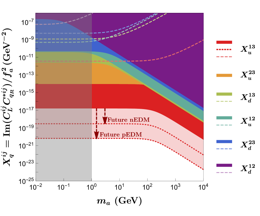
Figure -1018: ALP case. Bounds as a function of $m_{a}$. Upper bounds on $X_{q}^{ij}\equiv\operatorname{Im}\left(\bm{C}_{Q}^{ij}\bm{C}_{q_{R}}^{ij}\right)/f_{a}^{2}$ from the $\bar{\theta}$ correction (solid regions) and from qEDMs and cEDMs (dashed lines). Future bounds stemming from nEDM and pEDM projections  EuropeanStrategyforParticlePhysicsPreparatoryGroup:2019qin are indicated for $\bm{X}^{13}_{u}$ with a red dotted line. For ALP masses near or below the QCD threshold ($m_{a}\lesssim 1$ GeV, shaded region) the results are outside the validity of our approximations, see text.

Comparison with quark EDM contributions

Figure -1017: ALP-induced one loop contribution to the fermion-photon vertex as considered in Ref. DiLuzio:2020oah .

The Lagrangian in Eq. 1 also generates a contribution to the individual qEDMs $d_{u,d,s}$ and cEDMs $\tilde{d}_{u,d,s}$, which in turn contribute to the final nEDM value through Eq. (13). The corresponding Feynman diagram – see Fig. -1017 – has been previously computed DiLuzio:2020oah ; DasBakshi:2023lca , and for the up-quark EDM it contributes as

$$\frac{d_{u}}{e} \equiv\frac{Q_{u}}{32\pi^{2}f_{a}^{2}}\operatorname{Im}\left[\mathbf{C}_{Q}\bm{G}\,\mathbf{C}_{u_{R}}^{\dagger}\right]_{11}\,,$$ (16)

with $\bm{G}=\operatorname{diag}\left(G(x_{u}),\,G(x_{c}),\,G(x_{t})\right)$ and

$$G(x_{k}) \equiv m_{a}\,x_{k}^{3/2}\frac{(3-4\,x_{k}+x_{k}^{2}+2\,\log(x_{k}))}{(x_{k}-1)^{3}}$$

$$\sim\frac{m_{k}}{m_{a}^{2}}\texttt{min}(m_{a}^{2},3m_{k}^{2})\,,$$ (17)

where $x_{k}\equiv m_{k}^{2}/m_{a}^{2}$ , $Q_{u}=+2/3$ is the charge of the up-quark in units of $e$, and the last expression captures the order of magnitude for either $m_{a}\ll m_{k}$ or $m_{a}\gg m_{k}$. An analogous expression holds for the ALP induced $d_{d}$. Also, the same Feynman diagram depicts the one-loop contribution to the quark cEDM $\tilde{d}_{q}$ by replacing the photon with a gluon, and its computation can be simply recast from that for the qEDM as $\tilde{d}_{q}=d_{q}/e\,Q_{u,d}$, where the $g_{s}$ factor is customarily factored out in the definition, see Eq. (3).

The ${d}_{q}$ and $\tilde{d}_{q}$ contributions to the nEDM are comparable, and again the strongest bound corresponds to that involving the top quark in the loop,

$$\frac{\operatorname{Im}(\bm{C}_{Q}^{13}{\bm{C}_{u_{R}}^{*13}})}{f_{a}^{2}}\Bigg{|}_{{d}_{q},\,\tilde{d}_{q}}\lesssim 3.7\times 10^{-12}\,\text{GeV}^{-2}\,,$$ (18)

which is several orders of magnitude weaker than that obtained in Eq. 15 from ${\bar{\theta}}$.

$$\begin{array}[c]{ccc}\hbox{\multirowsetup\text{Combination}}&\text{$\bar{\theta}$-bounds}&\hbox{\multirowsetup\text{qEDM \& cEDM}}\\[-5.69054pt] &\text{{\small(GeV${}^{-2}$)}}&\text{{\small(GeV${}^{-2}$)}}\\[0.0pt] \hline\cr\\[-10.0pt] \operatorname{Im}[\bm{C}_{Q}^{13}\bm{C}_{u_{R}}^{*13}]/f_{a}^{2}&1.8\times 10^{-17}&3.7\times 10^{-12}\\[2.84526pt] \operatorname{Im}[\bm{C}_{Q}^{23}\bm{C}_{u_{R}}^{*23}]/f_{a}^{2}&1.1\times 10^{-14}&-\\[2.84526pt] \operatorname{Im}[\bm{C}_{Q}^{13}\bm{C}_{d_{R}}^{*13}]/f_{a}^{2}&1.1\times 10^{-12}&1.9\times 10^{-9}\\[2.84526pt] \operatorname{Im}[\bm{C}_{Q}^{12}\bm{C}_{u_{R}}^{*12}]/f_{a}^{2}&2.7\times 10^{-12}&2.3\times 10^{-9}\\[2.84526pt] \operatorname{Im}[\bm{C}_{Q}^{23}\bm{C}_{d_{R}}^{*23}]/f_{a}^{2}&2.3\times 10^{-11}&8.7\times 10^{-9}\\[2.84526pt] \operatorname{Im}[\bm{C}_{Q}^{12}\bm{C}_{d_{R}}^{*12}]/f_{a}^{2}&8.6\times 10^{-11}&1.2\times 10^{-5}\\[5.0pt] \hline\cr\end{array}$$

Table 2: ALP case. Bounds from ${\bar{\theta}}$ contributions versus qEDM and cEDM bounds. Experimental bounds on $\operatorname{Im}[\bm{C}_{Q}^{ij}\bm{C}_{q_{R}}^{*ij}]/f_{a}^{2}$ for the particular case $m_{a}=5$ GeV. The last column corresponds to the sum of the qEDM and cEDM contributions. The bounds can be extrapolated to other values of $m_{a}$ using Eq. (11) and Eq. (17), respectively.

Similarly, separate bounds on the other possible combinations of parameters can be obtained using Eqs. 13 and 17. As an example, in Table 2 we compare the bounds for the CP-odd combinations $X_{q}^{ij}\equiv\operatorname{Im}(\bm{C}_{Q}^{ij}\bm{C}_{q_{R}}^{ij})/f_{a}^{2}$ stemming from the qEDM and cEDM with those resulting from our analysis of the ${\bar{\theta}}$-parameter, for an ALP mass $m_{a}=5$ GeV. Fig. -1018 depicts, as a function of $m_{a}$, the bounds from ${\bar{\theta}}$ in solid regions and those from qEDM and cEDM with dashed lines. It is seen that, for $m_{a}\gtrsim 1$ GeV, the dominant bounds on $X^{ij}_{q}$ arise from the ALP contribution to $\bar{\theta}$. Notice as well that the qEDM and cEDM contributions do not allow to extract a bound on the combination $\operatorname{Im}[\bm{C}_{Q}^{23}\bm{C}_{u_{R}}^{*23}]/f_{a}^{2}$, while the $\bar{\theta}$ parameter is sensitive to it and leads to a strong bound (in blue).

We have cross-checked our results by performing the computation in an alternative basis, see Appendix A. Indeed, the chirality-preserving ALP-fermion interactions in Eq. 1 can be traded for a specific combination of Yukawa-like operators in the so-called “chirality-flip basis” via a suitable field redefinition of the fields. As this is only a change of basis, the number of free parameters does not change.

V Generic scalar with CP-odd fermionic interactions

Figure -1016: Scalar exchange one-loop contribution to the quark masses.

In this section, the previous analysis is extended to a theory of a singlet scalar $\phi$ with mass $m_{\phi}$ and coupled to SM fermions without imposing shift symmetry.

The most general CP-odd fermion-scalar interactions are described by a Lagrangian exhibiting Yukawa-like left-right interactions,

$$\mathcal{L} \supset\bar{u}_{L}\,v\,\left[i\,\bm{K}_{u}\frac{\phi}{\Lambda}\ +\bm{F}_{u}\frac{\phi^{2}}{\Lambda^{2}}\right]u_{R}$$

$$\hskip 28.45274pt+\bar{d}_{L}\,v\,\left[i\frac{\phi}{\Lambda}\bm{K}_{d}+\frac{\phi^{2}}{\Lambda^{2}}\bm{F}_{d}\right]d_{R}+\text{h.c.}$$ (19)

where $\bm{K}_{q}$ and $\bm{F}_{q}$ are arbitrary $3\times 3$ dimensionless coefficient matrices in flavour space and $\Lambda$ denotes the new physics scale. The dependence on the Higgs vacuum expectation value, $v=246$ GeV, is a remnant of the couplings ancestry above the electroweak scale, which corresponds to Yukawa-like operators of mass dimension 5 ($\bm{K}_{q}$ terms) and 6 ($\bm{F}_{q}$ terms). The $\mathcal{O}(1/\Lambda^{2}$) $\bm{F}_{q}$ terms have been included as this is required by the consistency of the EFT analysis at one-loop. They contribute to ${\bar{\theta}}$ through the lower diagram in Fig. -1016, at the same order as the first one (which presents two insertions of the coupling proportional to $\bm{K}_{d}/\Lambda$). Even considering only the $\bm{K}_{q}$ terms, this Lagrangian has more free parameters than that for the ALP in Eq. (1) (see also App. A). Those extra parameters include flavour-diagonal ones which can be complex, thus sourcing additional CP-violation effects, in contrast to the case of the ALP theory.

In the literature, it is also common to use the alternative notation

$$\bar{q}_{L}\,i\,v\,\frac{a}{f_{a}}\bm{K}_{q}\,q_{R}\equiv\frac{a}{f_{a}}\,v\,\left(\bar{q}\,\bm{y}_{qS}\,q+i\,\bar{q}\,\bm{y}_{qP}\gamma_{5}q\,\right)\,,$$ (20)

with

$$\bm{y}_{qS} \equiv i\,\frac{\bm{K}_{q}-\bm{K}_{q}^{\dagger}}{2}\,, \bm{y}_{qP} \equiv\frac{\bm{K}_{q}+\bm{K}_{q}^{\dagger}}{2}\,.$$ (21)

The contribution of the $\bm{K}_{q}$ and $\bm{F}_{q}$ parameters to ${\bar{\theta}}$ through its running reads:

$$\bar{\theta}\left(\mu_{IR}\right)\simeq{\bar{\theta}}_{0}+\frac{v^{2}}{16\pi^{2}\Lambda^{2}}\times\Bigg{(}\sum_{i,k}\bigg{[}\frac{m_{u_{k}}\operatorname{Im}\left(\bm{K}_{u}^{ik}\bm{K}_{u}^{ki}\right)}{m_{u_{i}}}-\frac{m_{\phi}^{2}\operatorname{Im}\left(\bm{F}_{u}^{ik}\right)}{m_{u_{i}}}\bigg{]}\log\frac{\Lambda^{2}}{\texttt{max}(m_{\phi}^{2},m_{u_{k}}^{2})}$$

$$\hskip 170.71652pt+\sum_{i,k}\bigg{[}\frac{m_{d_{k}}\operatorname{Im}\left(\bm{K}_{d}^{ik}\bm{K}_{d}^{ki}\right)}{m_{d_{i}}}-\frac{m_{\phi}^{2}\operatorname{Im}\left(\bm{F}_{d}^{ik}\right)}{m_{d_{i}}}\bigg{]}\log\frac{\Lambda^{2}}{\texttt{max}(m_{\phi}^{2},m_{d_{k}}^{2})}\Bigg{)}\,.$$ (22)

In turn, their contribution to the up-quark EDM is given by

$$\frac{d_{u}}{e} \equiv\frac{Q_{u}}{32\pi^{2}}\frac{v^{2}}{\Lambda^{2}}\operatorname{Im}\left[\mathbf{K}_{q}\bm{G^{\prime}}\,\mathbf{K}_{q}^{\dagger}\right]_{11}\,,$$ (23)

with $\bm{G}^{\prime}=\operatorname{diag}\left(G^{\prime}(x_{u}),\,G^{\prime}(x_{c}),\,G^{\prime}(x_{t})\right)$, where $x_{k}\equiv m_{k}^{2}/m^{2}_{\phi}$, and

$$G^{\prime}(x_{k}) \equiv\frac{x_{k}^{1/2}}{m_{\phi}}\frac{(3-4\,x_{k}+x_{k}^{2}+2\,\log(x_{k}))}{(x_{k}-1)^{3}}\,,$$

and analogously for the other flavours and for the quark cEDMs DiLuzio:2020oah .

Stringent restrictions on this enlarged $\{\bm{K}_{q},\bm{F}_{q}\}$ parameter space follow from the nEDM experimental limit Abel:2020pzs ; Afach:2015sja , with an impact comparable to that found in the previous sections for the CP-odd couplings of a generic ALP. Using again Eq. 13, the nEDM is seen to be sensitive to the combinations $W_{q}^{ij}\equiv\operatorname{Im}(\bm{K}_{q}^{ij}\bm{K}_{q}^{ji})/\Lambda^{2}$ and $V_{q}^{ii}\equiv\operatorname{Im}(\bm{F}_{q}^{ii})/\Lambda^{2}$. The corresponding bounds are displayed in Table 3 and depicted as a function of $m_{\phi}$ in Figs. -1015 and -1014. For most $W_{q}^{ij}$’s, the constraint imposed by their contribution to $\bar{\theta}$ dominates strongly over that from contributions to qEDMs and cEDMs. In addition, the contributions to $\bar{\theta}$ also provide a handle into several combinations of parameters —$W_{u}^{23}$, $W_{u}^{22}$, $W_{u,d}^{33}$ and the $V^{ii}_{q}$’s — which do not contribute to neither the qEDMs nor the cEDMs.

In summary, much as in the case of ALPS, the bounds obtained for a general scalar are several orders of magnitude stronger than those existing in the literature, due to the impact of the ${\bar{\theta}}$ parameter. Furthermore, some new combinations of parameters have become accessible via the present $\bar{\theta}$ analysis.

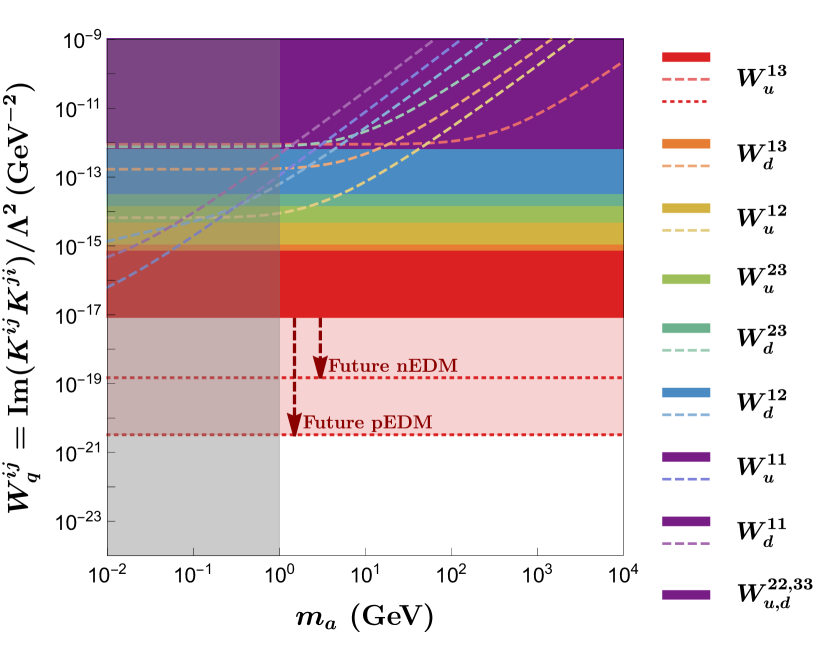
Figure -1015: General scalar. Upper bounds on $W_{q}^{ij}\equiv\operatorname{Im}(\bm{K}_{q}^{ij}\bm{K}_{q}^{ji})/\Lambda^{2}$ stemming from the contributions of $\bar{\theta}$ (solid regions) and from the sum of qEDMs and cEDMs (dashed lines) to the nEDM. The red dotted line shows the projected bounds on $W_{u}^{13}$ from future nEDM and pEDM experiments  Alexander:2022rmq ; Balashov:2007zj . The grey shaded area is as described in Fig. -1018.

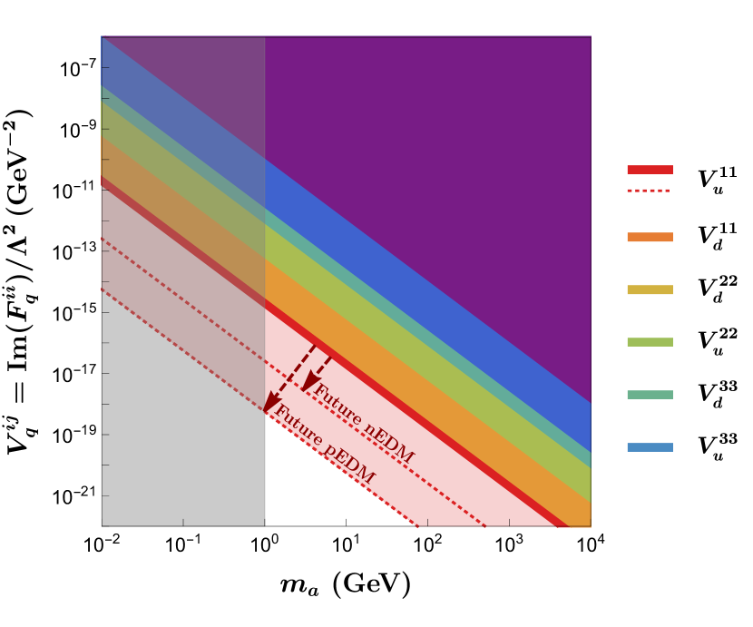
Figure -1014: General scalar. Upper bounds on $V_{q}^{ij}\equiv\operatorname{Im}\left(F_{q}^{ij}\right)/\Lambda^{2}$ stemming from the contributions of $\bar{\theta}$ (solid regions) to the nEDM. The red dotted line shows the projected bounds on $V_{u}^{11}$ from future nEDM and pEDM experiments Alexander:2022rmq ; Balashov:2007zj . The grey shaded area is as described in previous plots.

$$\begin{array}[c]{ccc}\hbox{\multirowsetup\text{Combination}}&\text{$\bar{\theta}$-bounds}&\hbox{\multirowsetup\text{qEDM \& cEDM}}\\[-5.69054pt] &\text{{\small(GeV${}^{-2}$)}}&\text{{\small(GeV${}^{-2}$)}}\\[0.0pt] \hline\cr\\[-10.0pt] \operatorname{Im}(\bm{K}_{u}^{13}\bm{K}_{u}^{31})/\Lambda^{2}&8.8\times 10^{-12}&9.0\times 10^{-7}\\[2.84526pt] \operatorname{Im}(\bm{K}_{d}^{13}\bm{K}_{d}^{31})/\Lambda^{2}&7.9\times 10^{-10}&2.8\times 10^{-7}\\[2.84526pt] \operatorname{Im}(\bm{K}_{u}^{12}\bm{K}_{u}^{21})/\Lambda^{2}&1.2\times 10^{-9}&3.1\times 10^{-8}\\[2.84526pt] \operatorname{Im}(\bm{K}_{u}^{23}\bm{K}_{u}^{32})/\Lambda^{2}&5.2\times 10^{-9}&-\\[2.84526pt] \operatorname{Im}(\bm{K}_{d}^{23}\bm{K}_{d}^{32})/\Lambda^{2}&1.6\times 10^{-8}&1.3\times 10^{-6}\\[2.84526pt] \operatorname{Im}(\bm{K}_{d}^{12}\bm{K}_{d}^{21})/\Lambda^{2}&3.5\times 10^{-8}&8.2\times 10^{-7}\\[2.84526pt] \operatorname{Im}(\bm{K}_{u}^{11}\bm{K}_{u}^{11})/\Lambda^{2}&7.1\times 10^{-7}&2.2\times 10^{-6}\\[2.84526pt] \operatorname{Im}(\bm{K}_{d}^{11}\bm{K}_{d}^{11})/\Lambda^{2}&7.1\times 10^{-7}&8.7\times 10^{-6}\\[2.84526pt] \operatorname{Im}(\bm{K}_{d}^{22}\bm{K}_{d}^{22})/\Lambda^{2}&7.1\times 10^{-7}&1.8\times 10^{-6}\\[2.84526pt] \operatorname{Im}(\bm{K}_{u}^{22}\bm{K}_{u}^{22})/\Lambda^{2}&7.1\times 10^{-7}&-\\[2.84526pt] \operatorname{Im}(\bm{K}_{u,d}^{33}\bm{K}_{u,d}^{33})/\Lambda^{2}&7.1\times 10^{-7}&-\\[2.84526pt] \operatorname{Im}(\bm{F}_{u}^{11})/\Lambda^{2}&6.1\times 10^{-11}&-\\[2.84526pt] \operatorname{Im}(\bm{F}_{d}^{11})/\Lambda^{2}&1.3\times 10^{-10}&-\\[2.84526pt] \operatorname{Im}(\bm{F}_{d}^{22})/\Lambda^{2}&2.6\times 10^{-9}&-\\[2.84526pt] \operatorname{Im}(\bm{F}_{u}^{22})/\Lambda^{2}&3.6\times 10^{-8}&-\\[2.84526pt] \operatorname{Im}(\bm{F}_{d}^{33})/\Lambda^{2}&1.2\times 10^{-7}&-\\[2.84526pt] \operatorname{Im}(\bm{F}_{u}^{33})/\Lambda^{2}&4.9\times 10^{-6}&-\\[5.69054pt] \hline\cr\end{array}$$

Table 3: General scalar. Bounds on $\operatorname{Im}(\bm{K}_{q}^{ij}\bm{K}_{q}^{ji})/\Lambda^{2}$ and $\operatorname{Im}(\bm{F}_{q}^{ii})/\Lambda^{2}$ stemming from their contribution to the nEDM. The bounds on $\operatorname{Im}(\bm{K}_{q}^{ij}\bm{K}_{q}^{ji})/\Lambda^{2}$ inferred from their contribution to $\bar{\theta}$ are independent of $m_{\phi}$, while those stemming from the sum of qEDMs and cEDMs are evaluated for $m_{\phi}=5$ GeV.

VI Discussion

In this work, we have computed the one-loop contribution to the $\bar{\theta}$-parameter of an ALP with CP-odd derivative couplings to fermions. Its impact on the nEDM is such that the bounds obtained on the CP-odd ALP-fermion couplings are many orders of magnitude stronger than those stemming from the contributions to up- and down-quark electric and chromo-electric dipole moments. The same conclusion applies to the CP-odd fermionic couplings of a generic scalar particle.

Finally, it is worth mentioning that the strong novel bounds found above, either for an ALP theory or for a general scalar, do not apply if those theories are extended by including in the Lagrangian –in addition to the ALP– an extra true QCD axion which solves the strong CP problem via a Peccei-Quinn mechanism. In that case, the QCD axion would absorb all contributions to ${\bar{\theta}}$ computed in this work. Still a non-zero induced ${\bar{\theta}}_{\text{ind}}$ Bigi:1991rh ; Pospelov:1999ha ; Pospelov:1997uv ; Pospelov:2000bw would remain, leading to weaker but significant bounds on the studied couplings Dekens:2022gha ; DiLuzio:2020oah . We expand on that case in Appendix C.

Acknowledgments.

—We thank Jesús Bonilla and María Ramos for illuminating discussions in the early stages of this project. We thank Jonathan Kley for pointing us to the most updated estimation of the qEDM contributions to the nEDM. We also thank Luca di Luzio and Maxim Pospelov for clarifications on their work. This project has received funding /support from the European Union’s Horizon 2020 research and innovation programme under the Marie Sklodowska-Curie grant agreement No. 860881-HIDDeN, and under the Marie Sklodowska-Curie Staff Exchange grant agreement No. 101086085-ASYMMETRY. The work of B.Gr. and P.Q. is supported in part by the U.S. Department of Energy Grant No. DE-SC0009919. The work of V.E. was supported by the Spanish MICIU through the National Program FPI-Severo Ochoa (grant number PRE2020-094281). B.Ga. and V. E. acknowledge as well partial financial support from the Spanish Research Agency (Agencia Estatal de Investigación) through the grant IFT Centro de Excelencia Severo Ochoa No CEX2020-001007-S, the grants PID2019-108892RB-I00 and PID2022-137127NB-I00 funded by MCIN/AEI/10.13039/501100011033/ FEDER, UE. B.Ga. and V. E. thank very much the Particle Physics group of the University of California, San Diego, where part of this work was carried out.

Appendix A Chirality-flip basis

As a double check and to facilitate the comparison of our results with the rest of the literature, we have also computed the ALP-fermion contribution to ${\bar{\theta}}$ in the chirality-flip basis. It is well-known Georgi:1986df ; Chala:2020wvs ; Bonilla:2021ufe that by applying the transformation

$$u_{L} \longrightarrow e^{i\frac{a}{f_{a}}\bm{C}_{Q}}u_{L}\,, d_{L} \longrightarrow e^{i\frac{a}{f_{a}}\bm{C}_{Q}}d_{L}\,,$$ (24)

$$u_{R} \longrightarrow e^{i\frac{a}{f_{a}}\bm{C}_{u_{R}}}u_{R}\,, d_{R} \longrightarrow e^{i\frac{a}{f_{a}}\bm{C}_{d_{R}}}d_{R}\,$$ (25)

to the Lagrangian in Eq. 1 one can trade the derivative ALP-fermionic interactions by Yukawa-like left-right interactions as described by

$$\mathcal{L} \supset\bar{u}_{L}\,v\,\left[i\frac{a}{f_{a}}\bm{K}_{u}+\frac{a^{2}}{f_{a}^{2}}\bm{F}_{u}\right]u_{R}$$

$$\hskip 28.45274pt+\bar{d}_{L}\,v\,\left[i\frac{a}{f_{a}}\bm{K}_{d}+\frac{a^{2}}{f_{a}^{2}}\bm{F}_{d}\right]d_{R}+\text{h.c.}+\dots$$ (26)

where the $\bm{K}_{q}$ and $\bm{F}_{q}$ coefficient matrices are given by

$$\begin{aligned} v\,\bm{K}_{q}&\equiv\bm{C}_{Q}\bm{M}_{q}-\bm{M}_{q}\bm{C}_{q_{R}}\,,\\ 2\,v\,\bm{F}_{q}&\equiv 2\bm{C}_{Q}\bm{M}_{q}\bm{C}_{q_{R}}-\bm{C}_{Q}^{2}\bm{M}_{q}-\bm{M}_{q}\bm{C}_{q_{R}}^{2}\,,\end{aligned}$$ (27)

and the ellipsis stands for higher order terms $\mathcal{O}(1/f_{a}^{3})$.

The Lagrangian in Eq. (26) is formally the same than that in Eq. (19) for a general scalar (with the replacement $\phi\to a$ and $\Lambda\to f_{a}$), but the relations in Eq. (27) reduce its degrees of freedom. They ensure that it is shift-symmetric under $a\to a+\rm{constant}$ and equivalent to the ALP Lagrangian in Eq.(1).

In this chirality-flip basis the two diagrams in Fig. -1016 contribute to the one-loop corrections to the quark masses (in contrast with the derivative basis where only the first topology contributes). It is straightforward to check that the result obtained in the derivative basis, Eq. 12, is recovered by substituting Eq. 27 into Eq. 22.

Appendix B nEDM estimates from QCD sum rules without a Peccei-Quinn symmetry

Various methods, including naive dimensional analysis Manohar:1983md , chiral lagrangians Crewther:1979pi ; Guo:2012vf , lattice simulations Gupta:2018lvp and QCD sum rules Shifman:1978bx ; Pospelov:2005pr can be employed to obtain estimates of the nEDM and pEDM as a function of $\bar{\theta},\,d_{q}$ and $\tilde{d}_{q}$. Their corresponding results do not always agree with each other and present a large span of uncertanties.

Thoughout this paper we will use the lattice result in Ref. Gupta:2018lvp for the coefficients of the qEDMs in the nEDM and pEDM formulae,

$$d_{n}(d_{q}) =-0.204(11)\,d_{u}+0.784(28)\,d_{d}-0.0028(17)\,d_{s}$$

$$d_{p}(d_{q}) =+0.784(28)\,d_{u}-0.204(11)\,d_{d}-0.0028(17)\,d_{s}$$ (28)

Note that the estimation in Ref. DiLuzio:2020oah has a typographical error as the numerical coefficients for $d_{u}$ and $d_{d}$ appear interchanged with respect to the lattice results in Ref. Gupta:2018lvp .

For the rest of the coefficients $d_{n}(\bar{\theta},\tilde{d}_{q})$ we will use the analytical formulas from QCD sum rule estimates in Ref. Hisano:2012cc for the nEDM. The formula for $d_{p}(\bar{\theta},\tilde{d}_{q})$ is obtained by interchanging $u\leftrightarrow d$ in $d_{n}(\bar{\theta},\tilde{d}_{q})$. The result reads

$$d_{n,p}\left(\bar{\theta},\tilde{d}_{q},d_{q}\right)=-c_{0}\frac{\langle\bar{q}q\rangle}{\lambda_{N}^{2}m_{n,p}}{\Theta_{n,p}}\left(\bar{\theta},\tilde{d}_{q},d_{q}\right),$$ (29)

where $c_{0}=1.8\times 10^{-2}\,{\rm GeV}^{4}$ Hisano:2012cc , $m_{n,p}$ respectively denote the neutron and proton mass, the value of the chiral condensate will be taken from the recent computation in Ref. Gubler:2018ctz $\langle\bar{q}q\rangle=-(0.272(5)\mathrm{GeV})^{3}$ and the low-energy constant $\lambda_{N}=-0.0436(131)\mathrm{GeV}^{3}$ will be taken from a lattice calculation Hisano:2012cc . The ${\Theta_{n,p}}$ functions are given by

$$\Theta_{n}\left(\bar{\theta},\tilde{d}_{q},d_{q}\right) =\chi m_{*}\left[\left(4e_{d}-e_{u}\right)\left(\bar{\theta}-\frac{m_{0}^{2}}{2}\frac{\tilde{d}_{s}}{m_{s}}\right)+\frac{m_{0}^{2}}{2}\left(\tilde{d}_{d}-\tilde{d}_{u}\right)\left(\frac{4e_{d}}{m_{u}}+\frac{e_{u}}{m_{d}}\right)+\frac{m_{0}^{2}}{2}\,\left(\frac{4\,e_{d}}{m_{s}}\tilde{d}_{d}-\frac{e_{u}}{m_{s}}\tilde{d}_{u}\right)\right]+$$

$$\hskip 256.0748pt+\big{(}\kappa-\frac{1}{2}\xi\big{)}\left(4e_{d}\tilde{d}_{d}-e_{u}\tilde{d}_{u}\right)+\left(4d_{d}-d_{u}\right)\,,$$

$$\Theta_{p}\left(\bar{\theta},\tilde{d}_{q},d_{q}\right) =\chi m_{*}\left[\left(4e_{u}-e_{d}\right)\left(\bar{\theta}-\frac{m_{0}^{2}}{2}\frac{\tilde{d}_{s}}{m_{s}}\right)+\frac{m_{0}^{2}}{2}\left(\tilde{d}_{u}-\tilde{d}_{d}\right)\left(\frac{4e_{u}}{m_{d}}+\frac{e_{d}}{m_{u}}\right)+\frac{m_{0}^{2}}{2}\,\left(\frac{4\,e_{u}}{m_{s}}\tilde{d}_{u}-\frac{e_{d}}{m_{s}}\tilde{d}_{d}\right)\right]+$$

$$\hskip 256.0748pt+\big{(}\kappa-\frac{1}{2}\xi\big{)}\left(4e_{u}\tilde{d}_{u}-e_{d}\tilde{d}_{d}\right)+\left(4d_{u}-d_{d}\right)\,.$$ (30)

where $m_{*}\equiv\big{(}1/m_{u}+1/m_{s}+1/m_{s}\big{)}^{-1}$, $e_{u}$ and $e_{d}$ denote the electromagnetic charges of the up and down quarks ($e_{u}=+2/3\,e\,,\,e_{d}=-1/3\,e$) and the parameters $m_{0}^{2}=0.8(2)\,\mathrm{GeV}^{2},$ $\kappa=-0.34(10)$, $\chi=-5.7(6)\,\mathrm{GeV}^{-2}$ Belyaev:1982sa ; Ioffe:1983ju and $\xi=-0.74(20)$ Khatsymovsky:1990jb ; Kogan:1991en are as defined in Eqs. (48-50) in Ref. Hisano:2012cc . Substituting these input parameters in Eqs. 29 and 30 we finally obtain:

$$d_{n}(\bar{\theta},\tilde{d}_{q},d_{q}) ={0.6(3)\times 10^{-16}\,\bar{\theta}[e\cdot\mathrm{cm}]}$$ (31)

$$-0.2(1)\,d_{u}+0.8(4)\,d_{d}-0.0028(17)\,d_{s}$$

$${-0.32(16)\,e\,\tilde{d}_{u}+0.32(16)\,e\,\tilde{d}_{d}-0.014(7)\,e\,\tilde{d_{s}}\,,}$$

$$d_{p}(\bar{\theta},\tilde{d}_{q},d_{q}) =-1.0(5)\times 10^{-16}\,\bar{\theta}[e\cdot\mathrm{cm}]$$ (32)

$$+0.8(4)\,d_{u}-0.2(1)\,d_{d}-0.0028(17)\,d_{s}$$

$${-0.26(13)\,e\,\tilde{d}_{u}+0.28(14)\,e\,\tilde{d}_{d}+0.02(1)\,e\,\tilde{d}_{s}}\,.,$$

Note that the coefficients of the qEDMs predicted from these QCD sum rules, with the updated the input values we use, are in good agreement with the lattice QCD result in Eq. 28. The difference between our numerical results in Eq. 31 and (32) and those in Hisano:2012cc result solely because we use an updated value for the quark condensate. Note that the apparent discrepancy in the powers of $m_{n}$ in Eq. 29 with respect to the expression in Ref.Hisano:2015rna results from the fact that the definition of the $c_{0}$ coefficient in Ref. Hisano:2012cc (and our results) differs by a factor of $m_{n}^{4}$ with respect to that in Ref. Hisano:2015rna .

Appendix C nEDM estimates in the presence of a Peccei-Quinn symmetry

The presence of a Peccei-Quinn symmetry (with its corresponding QCD axion) modifies the nEDM estimates in Eq. 13. Firstly, the vev of the QCD axion will cancel the direct ${\bar{\theta}}$ dependence in the first term of Eq. 13. Secondly, the presence of explicit CP violation, e.g. via dipole moment couplings, shifts the minimum of the QCD axion potential away from the CP-conserving minimum, generating an induced ${\bar{\theta}}_{\rm ind}$ Bigi:1991rh ; Pospelov:1999ha ; Pospelov:1997uv ; Pospelov:2000bw . Indeed, for a chiral CP-odd theory such as that under consideration in Eq. 1, the Vafa-Witten Vafa:1983tf theorem does not apply and therefore cannot guarantee that the minimum of the axion sits exactly at the CP-conserving minimum. The value of ${\bar{\theta}}_{\rm ind}$ is dominated by the cEDM Pospelov:1997uv ,

$${\bar{\theta}}_{\text{ind }}=\frac{m_{0}^{2}}{2}\sum_{q=u,d,s}\frac{\tilde{d}_{q}}{m_{q}}\,,$$ (33)

where our sign convention for $m_{0}^{2}$ is that of belyaev1982 . Taking this induced $\bar{\theta}_{\text{ind}}$ into account results into a modification of the coefficients in Eqs. 13 and 14 which now read Pospelov:2005pr ; Cirigliano:2019vfc

$$d_{n}^{\rm PQ} =-0.204(11)d_{u}+0.784(28)d_{d}$$

$$\hskip 28.45274pt-0.31(15)e\,\tilde{d}_{u}+0.62(31)\,e\,\tilde{d}_{d}\,,$$ (34)

$$d_{p}^{\rm PQ} =0.784(28)d_{u}-0.204(11)d_{d}$$

$$\hskip 28.45274pt-1.21(60)\,e\,\tilde{d}_{u}-0.15(7)\,e\,\tilde{d}_{d}$$ (35)

This result was obtained by substituting, in the estimation of Eq. 13, ${\bar{\theta}}$ by the expression for ${\bar{\theta}}_{\rm ind}$ in Eq. 33, i.e. $d_{n,p}^{\rm PQ}(d_{u,d},\tilde{d}_{u,d})=d_{n,p}({\bar{\theta}}={\bar{\theta}}_{\rm ind},d_{u,d},\tilde{d}_{u,d})$. It differs from the result in Ref. Pospelov:2005pr because we are using a more refined estimation of $d_{n,p}({\bar{\theta}})$ Guo:2012vf . Note that in these two equations the dependence on the qEDMs did not suffer any modification with respect to the estimation without PQ symmetry in Eqs. (13) and (14) since the induced ${\bar{\theta}}_{\rm ind}$ due to the existence of the qEDM is negligible Pospelov:1997uv , while the impact on the cEDMs is significant as earlier explained.

The resulting bounds on ALP-fermion CP-odd couplings are shown in Table 4 for the case of an ALP with derivative couplings, and in Table 5 for the case of a general scalar. In the latter case no bounds results on the $\operatorname{Im}(\bm{F}_{q}^{ii})/\Lambda^{2}$ coefficients, as their contribution is completely reabsorbed away by the Peccei-Quinn symmetry.

Combination	With PQ	Without PQ
	(GeV-2)	(GeV-2)
$\operatorname{Im}(\bm{C}_{L}^{13}\bm{C}_{u_{R}}^{13})/f_{a}^{2}$	$3.7\times 10^{-12}$	$3.7\times 10^{-12}$
$\operatorname{Im}(\bm{C}_{L}^{13}\bm{C}_{d_{R}}^{13})/f_{a}^{2}$	$1.9\times 10^{-9}$	$3.2\times 10^{-9}$
$\operatorname{Im}(\bm{C}_{L}^{12}\bm{C}_{u_{R}}^{12})/f_{a}^{2}$	$2.3\times 10^{-9}$	$2.4\times 10^{-9}$
$\operatorname{Im}(\bm{C}_{L}^{23}\bm{C}_{d_{R}}^{23})/f_{a}^{2}$	$8.7\times 10^{-9}$	$1.2\times 10^{-7}$
$\operatorname{Im}(\bm{C}_{L}^{12}\bm{C}_{d_{R}}^{12})/f_{a}^{2}$	$1.2\times 10^{-5}$	$1.9\times 10^{-6}$

Table 4: ALP case. Comparison of bounds w/o the presence of a PQ symmetry. All bounds are in units of GeV^-2, and $m_{a}=5$ GeV has been assumed for illustration.

$$\begin{array}[c]{ccc}\hbox{\multirowsetup\text{Combination}}&\text{With PQ}&\hbox{\multirowsetup\text{Without PQ}}\\[-2.84526pt] &\text{{\small(GeV${}^{-2}$)}}&\text{{\small(GeV${}^{-2}$)}}\\[0.0pt] \hline\cr\\[-10.0pt] \operatorname{Im}(\bm{K}_{u}^{13}\bm{K}_{u}^{31})/\Lambda^{2}&9.0\times 10^{-7}&9.2\times 10^{-7}\\[2.84526pt] \operatorname{Im}(\bm{K}_{d}^{13}\bm{K}_{d}^{31})/\Lambda^{2}&2.8\times 10^{-7}&4.6\times 10^{-8}\\[2.84526pt] \operatorname{Im}(\bm{K}_{u}^{12}\bm{K}_{u}^{21})/\Lambda^{2}&3.1\times 10^{-8}&3.1\times 10^{-8}\\[2.84526pt] \operatorname{Im}(\bm{K}_{d}^{23}\bm{K}_{d}^{23})/\Lambda^{2}&1.3\times 10^{-6}&1.8\times 10^{-5}\\[2.84526pt] \operatorname{Im}(\bm{K}_{d}^{12}\bm{K}_{d}^{21})/\Lambda^{2}&8.2\times 10^{-7}&1.4\times 10^{-7}\\[2.84526pt] \operatorname{Im}(\bm{K}_{d}^{22}\bm{K}_{d}^{22})/\Lambda^{2}&3.8\times 10^{-6}&5.3\times 10^{-5}\\[2.84526pt] \operatorname{Im}(\bm{K}_{u}^{11}\bm{K}_{u}^{11})/\Lambda^{2}&2.2\times 10^{-6}&2.2\times 10^{-6}\\[2.84526pt] \operatorname{Im}(\bm{K}_{d}^{11}\bm{K}_{d}^{11})/\Lambda^{2}&8.7\times 10^{-6}&1.4\times 10^{-6}\\[2.84526pt] \hline\cr\hline\cr\end{array}$$

Table 5: General scalar. Comparison of bounds w/o the presence of a PQ symmetry. All bounds are in units of GeV^-2, and for $m_{\phi}=5$ GeV.

Appendix D Leading Logs in the quark mass running

Consider integration of Eq. 10 retaining dependence on the QCD coupling, $\alpha_{s}$, so that the effect of running masses is retained. We neglect electroweak interactions since their effect is much smaller. To incorporate these effects we solve Eq. 10 making use of the explicit derivative

$$\mu\frac{d}{d\mu}=\mu\frac{\partial}{\partial\mu}+\beta(g_{s})\frac{\partial}{\partial g_{s}}+\sum_{q}m_{q}\gamma_{m}(g_{s})\frac{\partial}{\partial m_{q}}$$ (36)

and the observation that the couplings $\mathbf{C}_{L,u_{R},d_{R}}$ have vanishing anomalous dimensions, because the corresponding operators in the Lagrangian of Eq. 1 are partially conserved currents in QCD. Denoting by $\bar{g}$ and $\bar{m}$ the running coupling and quark mass in QCD, that is the solutions to

$$\mu\frac{d\bar{g}}{d\mu}=\beta(\bar{g})\quad\text{and}\quad\mu\frac{d\overline{m}}{d\mu}=\gamma_{m}(\bar{g})\overline{m}\,,$$

integration of Eq. 10 including the full $\mu$-derivative of Eq. 36 is equivalent to using only the $\mu\partial{\bar{\theta}}/\partial\mu$ on the left hand side and substituting running couplings for the couplings on the right hand side.

Leading-log resummation is achieved using one-loop running couplings. Using

$$\beta(g)=-b_{0}\frac{g^{3}}{16\pi^{2}}\quad\text{and}\quad\gamma_{m}(g)=a_{m}\frac{g^{2}}{16\pi^{2}}$$

with $b_{0}=11-2n_{f}/3$ and $a_{m}=-8$ , the running couplings $\overline{\alpha}_{s}(\mu)$ are

$$\frac{1}{\overline{\alpha}_{s}(\mu)}-\frac{1}{\overline{\alpha}_{s}(\mu^{\prime})}=\frac{b_{0}}{2\pi}\ln(\mu/\mu^{\prime})$$ (37)

and

$$\overline{m}(\mu)=\overline{m}(\mu^{\prime})\left(\frac{\bar{\alpha}_{s}(\mu)}{\bar{\alpha}_{s}(\mu^{\prime})}\right)^{-a_{m}/2b_{0}}\,.$$ (38)

Notice that the running of the factor of $\mathbf{M}^{-1}$ on the right hand side on Eq. 10 cancels with the explicit overall mass factor in $\mathcal{L}$ of Eq. 11. What remains is an integral over $m_{a}^{2}+m_{q}^{2}$. The first of these is $\mu$-independent so that integration simply gives a logarithm of the ratio of scales, as in Eq. 12. For the second term one needs

$$\int_{\mu^{\prime}}^{\mu}\frac{d\mu}{\mu}\overline{m}^{2}=\int_{g^{\prime}}^{g}\frac{d\bar{g}}{\beta(\bar{g})}\overline{m}(\bar{g})^{2}=-\frac{16\pi^{2}}{b_{0}}\overline{m}^{2}(\mu^{\prime})\int_{g^{\prime}}^{g}\frac{d\bar{g}}{\bar{g}^{3}}\left(\frac{g^{\prime}}{\bar{g}}\right)^{2a_{m}/b_{0}}=\frac{8\pi^{2}}{b_{0}(1+a_{m}/b_{0})}\left(\frac{\overline{m}^{2}(\mu)}{\bar{g}^{2}(\mu)}-\frac{\overline{m}^{2}(\mu^{\prime})}{\bar{g}^{2}(\mu^{\prime})}\right)\,.$$

In the limit of vanishing coupling, $g\to 0$ this gives $m^{2}\ln(\mu/\mu_{0})$, reproducing the explicit log in Eq. 12. Accordingly one should use

$$\hat{m}^{2}_{q_{k}}\log(\mu_{0}^{2}/\mu_{1}^{2})=\frac{4\pi}{b_{0}(1+a_{m}/b_{0})}\left(\frac{\overline{m}^{2}(\mu_{0})}{\overline{\alpha}_{s}(\mu_{0})}-\frac{\overline{m}^{2}(\mu_{1})}{\overline{\alpha}_{s}(\mu_{1})}\right)\,,$$ (39)

with $\mu_{0}=f_{a}$ and $\mu_{1}=\texttt{max}(m_{a}^{2},m_{d_{k}}^{2})$ in Eq. 12.

A couple of remarks are in order. First, when computing the ratios $m_{u_{k}}/m_{u_{i}}=\overline{m}_{u_{k}}(\mu)/\overline{m}_{u_{i}}(\mu)$ and $m_{d_{k}}/m_{d_{i}}=\overline{m}_{d_{k}}(\mu)/\overline{m}_{d_{i}}(\mu)$ at a common renormalization scale $\mu$, the running of the mass and coupling constant may change as they cross through thresholds. For example, for the $m_{u_{k}}/m_{u_{i}}=m_{t}/m_{u}$ case one writes the ratio in terms of $\overline{m}_{t}(m_{t})$ and $\overline{m}_{u}(\mu_{IR})$ with $\mu_{IR}=\text{2\;GeV}$, the values at the scales where they are often reported, as

$$\frac{m_{t}}{m_{u}}=\left(\frac{\overline{\alpha}^{(5)}_{s}(m_{t})}{\overline{\alpha}^{(5)}_{s}(m_{b})}\right)^{\frac{12}{23}}\left(\frac{\overline{\alpha}^{(4)}_{s}(m_{b})}{\overline{\alpha}^{(4)}_{s}(\mu_{IR})}\right)^{\frac{12}{25}}\frac{\overline{m}_{t}(m_{t})}{\overline{m}_{u}(\mu_{IR})}$$

where $\overline{\alpha}_{s}^{(n_{f})}(\mu)$ is the running coupling of Eq. 37 computed with $n_{f}$ active quark flavours. And second, similarly, the effective mass in Eq. 39 accounts for threshold effects additively. For example, if $m_{a}<m_{b}$ one should use

$$\widehat{m}^{2}_{b}\log(\mu_{0}^{2}/m_{b}^{2})=4\pi\overline{m}_{b}^{2}(m_{b})\left[\left(\frac{\overline{\alpha}^{(5)}_{s}(m_{t})}{\overline{\alpha}^{(5)}_{s}(m_{b})}\right)^{\frac{24}{23}}\left(\frac{1}{\overline{\alpha}^{(6)}_{s}(m_{t})}-\frac{1}{\overline{\alpha}_{s}^{(6)}(\mu_{0})}\left(\frac{\overline{\alpha}^{(6)}_{s}(\mu_{0})}{\overline{\alpha}^{(6)}_{s}(m_{t})}\right)^{\frac{24}{21}}\right)\right.\\ \left.+3\left(\frac{1}{\overline{\alpha}^{(5)}_{s}(m_{b})}-\frac{1}{\overline{\alpha}_{s}^{(5)}(m_{t})}\left(\frac{\alpha^{(5)}_{s}(m_{t})}{\alpha^{(5)}_{s}(m_{b})}\right)^{\frac{24}{23}}\right)\right]\,.$$ (40)

To get a sense of the magnitude of the leading log (LL) resummation we take $m_{a}<m_{t}$ and $f_{a}=10^{8}\;\text{GeV}$ which would be the minimum required from our conservative bounds in Table 1 for $\operatorname{Im}[\bm{C}_{L}^{13}\bm{C}_{u_{R}}^{*13}]\sim 10^{-2}$. Then we use, naively, $\widehat{m}_{q}=\overline{m}_{q}(m_{q})$ and then compare both sides of Eq. 39 and of Eq. 40. Using $\overline{\alpha}_{s}^{(5)}(M_{z})=0.12$, $m_{t}=175\;\text{GeV}$, $m_{b}=4.2\;\text{GeV}$ we obtain that the naive log overestimates the LL by factors of 1.8 and 2.8 in Eq. 39 and Eq. 40, respectively. It is a curious coincidence that the running of the up-quark from 1.0 GeV to $m_{t}$ required to compute the factor $m_{t}(m_{t})/m_{u}(m_{t})$ in Eq. 12 is 1.8, exactly compensating for the LL resummation:

$$\frac{\overline{m}_{t}(m_{t})}{\overline{m}_{u}(1\;\text{GeV})}\overline{m}_{t}^{2}(m_{t})\approx\frac{\overline{m}_{t}(m_{t})}{\overline{m}_{u}(m_{t})}\widehat{m}_{t}^{2}$$

This coincidence is not generic; the running of the $d$ or $s$ quark masses from 1.0 GeV to $m_{b}$ gives an enhancement of 1.3 to the ratio $m_{b}/m_{d,s}$, so the overall LL resummation effect is a a factor of 2.1 suppression.

We hasten to remind the reader that the bounds on couplings in Sec. IV use, conservatively, $\widehat{m}_{q}^{2}\log(f_{a}^{2}/\mu_{1}^{2})\to m_{q}^{2}$, with $m_{q}=\overline{m}_{q}(m_{q})$ for $q=t,b,c$ and $\overline{m}_{q}(1\;\text{GeV})$ for $q=u,d,s$. For the parameters chosen in the examples above the neglected logarithmic factor is $\sim 20$. It goes without saying that including this rather large logarithmic factor results in stronger bounds than the ones we obtained.