Mono- and oligochromatic extreme-mass ratio inspirals

Abstract

The gravitational capture of a stellar-mass object by a supermassive black hole represents a unique probe of warped spacetime. The small object, typically a stellar-mass black hole, describes a very large number of cycles before crossing the event horizon. Because of the mass difference, we call these captures extreme-mass ratio inspirals (EMRIs). Their merger event rate at the Galactic Centre is negligible, but the amount of time spent in the early inspiral is not. Early EMRIs (E-EMRIs) spend hundreds of thousands of years in band during this phase. At very early stages, the peak of the frequency will not change during an observational time. At later stages in the evolution, it will change a bit and finally the EMRI explores a wide range of them when it close to merger. We distinguish between “monocromatic” E-EMRIs, which do not change their (peak) frequency, oligochromatic E-EMRIs, which explore a short range and polychromatic ones, the EMRIs which have been discussed so far in the literature. We derive the number of E-EMRIs at the Galactic Centre, and we also calculate their signal-to-noise ratios (SNR) and perform a study of parameter extraction. We show that parameters such as the spin and the mass can be extracted with an error which can be as small as $10^{-11}$ and $10^{-5}\,M_{\odot}$. There are between hundreds and thousands of E-EMRIs in their monochromatic stage at the GC, and tens in their oligochromatic phase. The SNR ranges from a minimum of $10$ (larger likelihood) to a maximum of $10^{6}$ (smaller likelihood). Moreover, we derive the contribution signal corresponding to the incoherent sum of continuous sources of oligochromatic E-EMRIs with two representatives masses; $10\,M_{\odot}$ and $40\,M_{\odot}$ and show that their curves will cover a significant part of LISA’s sensitivity curve. Depending on their level of circularisation, they might be detected as individual sources or form a foreground population.

I Introduction

When a stellar-mass compact object such as a white dwarf, a neutron star or, more likely due to mass segregation, a black hole forms a binary with a supermassive one (MBH), the system radiates energy in gravitational waves (Einstein, 1916, 1918). The large mass-ratio of the system is large, ranging between $10^{6}$ for a neutron star or white dwarf forming a binary with a MBH of mass $10^{6}\,M_{\odot}$, to $10^{5}$ for a stellar-mass blach hole of $10\,M_{\odot}$. Therefore we call these systems extreme-mass ratio inspirals (Amaro-Seoane, 2018a; Amaro Seoane, 2022; Amaro-Seoane et al., 2007), and they constitute one of the main targets of the Laser Interferometer Space Antenna (LISA Amaro-Seoane et al., 2017). We can envisage these sources as a kind of camera taking snapshots of warped spacetime around a MBH. They will allow us to probe very closely the event horizon of the MBH and the geometry of spacetime in this regime of strong gravity (Amaro-Seoane et al., 2015).

The timescale associated to a gravitational-wave source can be approximated thanks to the work of Peters (1964). This timescale has the strongest dependency with the semimajor axis of the binary, which is to the power of four, i.e. $T\propto a^{4}$. The binary will hence spend most of its lifetime in the early phases of the inspiral, to then “accelerate” towards the merger and ringdown. Moreover, the number of cycles that a binary spends is roughly proportional to the mass ratio of the two compact objects (see, e.g. Maggiore, 2018, 2008). In the case of an EMRI, this number can be as large as $10^{7}$ if we consider a MBH of mass $10^{7}\,M_{\odot}$ and a neutron star. This means that an EMRI can spend, as we will see, up to $10^{5}$ years in the band of the detector if we consider a stellar-mass black hole.

Depending on their evolution stage, i.e. how far they are from plunging through the event horizon, they will evolve little or nothing in frequency. They are early-stage EMRIs (E-EMRIs), which have a complete different behavour as compared to late-type ones, the ones we have been talking about all along. Depending on their evolution stage, we call them (1) “monochromatic”, meaning that the peak of frequencies will not evolve for the observational time (but obviously the sources will have a spread of harmonics), (2) oligochromatic, i.e. they explore a short range of frequencies which however is significantly smaller than that of (3) polychromatic EMRIs, the sources which have been studied in detail until now in the literature.

Even though the merger event rate (i.e. how many of them cross the event horizon of the supermassive black hole) can be as low as $10^{-6}\text{yr}^{-1}$ for our Milky Way (Amaro-Seoane, 2019), because of the time spent in the detection band, what matters is the total number of E-EMRIs. This can be derived by multiplying the event rate times the lifetime of the binary with a signal-to-noise ratio (SNR) above a detection threshold, which we set to 10 in this work.

We find that in our Milky Way, at any given moment, there are hundreds of E-EMRIs as far as $10^{5}$ years from plunge fulfilling this requirement, and that they can achieve SNRs $\gtrsim 10^{3}$ tens of thousands of years before the plunge. Using “realistic” waveforms (i.e. not just the quadrupole, but based in the work of (Barack and Cutler, 2004a, b)), we do a Fisher matrix parameter study and find that we can obtain the spin and mass of SgrA* with a negligible errors, as small as $10^{-11}$ and $10^{-5}\,M_{\odot}$, respectively. As a side note, we calculate the asymptotic behaviour of the quadrupole approximation when the eccentricity tends to 1 and find that the equations in the work of (Peters, 1964) coincides with the asymptotic solution for eccentricities as large as $e=0.99999$ and higher.

We additionally calculate the incoherent contribution of individual E-EMRIs per bin of frequency with the proviso that they are continuous. This means that, from the population of thousands of E-EMRIs, we only select those which have a continuous signal. To illustrate this, we consider a population of only two masses, $10$ and $40\,M_{\odot}$. Because we are taking into account only continuous signals, from the thousands of sources we are left with about 160 of them. These nonetheless are sufficient to build up a foreground signal which can cover a significant fraction of LISA’s sensitivity area, between $10^{-4}$ to $3\times 10^{-3}$ Hz and from $10^{-16}$ to $10^{-21}$ in the characteristic strain.

Depending on (1) the mission duration, which affects the binning in frequency, and (2) the stage in their evolution, some of the sources will be resolved individually. In this work, however, we are limited to a binning of $10^{-5}$ Hz to depict the incoherent contribution. A narrower binning interval would render the computational calculations much more intensive and is hence not included in this study.

It is important to note that discontinuous sources will however also contribute at the Galactic Centre. These sources will spend only a fraction of their orbit in the LISA band, and might enter and leave the band in a repeated fashion. Because of this, we dub them as “popcorn EMRIs”. Even if they correspond to non-continuous signals, it is possible to calculate their Fourier transform via Schwarz functions. We will address these sources and their contribution elsewhere, in a separate work.

II EMRI waveforms with extreme eccentricities: SNR calculation and parameter extraction

To understand how E-EMRIs located at the Galactic Centre appear in the observatory band, in this section we first make an analysis by decomposing the approximate quadrupole waveform into harmonics. The advantage of this technique is that it gives us relevant information regarding the evolution as a function of frequency that is hidden if we represent the source with the full waveform. We hence approximate the source as a Keplerian ellipse which only changes over time due to the emission of energy (Peters, 1964). I.e. it shrinks but we do not take into account the periapsis shift, nor the effects of the spin of SgrA*. However simplified, this first study allows us to understand the relevance of E-EMRIs. Later we address more complex waveforms which require a computational analysis. Thanks to them we perform a Fisher matrix study and extract the parameters for a few representative examples.

II.1 A first study via Keplerian ellipses

From the work of (Peters, 1964) we can do a first analysis if we take into account that at a given distance $D$, a source of gravitational radiation emitting a given power $P$ and with a varying frequency $\dot{f}$ has a characteristic strain which can be expressed as a sum of harmonics $h_{\rm c,\,n}={(2\dot{E}_{n}/\dot{f}_{n})}^{1/2}/(\pi D)$, as described by Finn and Thorne (2000); Barack and Cutler (2004a, b), with $\dot{E}_{n}$ the power radiated to infinity in gravitational waves at a given frequency $f_{n}=n\,\nu$, and $n$ an integer larger than 0. Therefore, the contribution of each harmonic $n$ is given by

$$h_{c,\,n} =\frac{G^{2}\,M_{\rm BH}m_{*}}{D\,ac^{4}}\left(\frac{n^{4}}{32}\right)\Bigg{\{}\Big{[}J_{n-2}(ne)-2eJ_{n-1}(ne)$$

$$+\frac{2}{n}J_{n}(ne)+2eJ_{n+1}(ne)-J_{n+2}(ne)\Big{]}^{2}$$

$$+\left(1-e^{2}\right)\Big{[}J_{n-2}(ne)-2J_{n}(ne)+J_{n+2}(ne)\Big{]}^{2}$$

$$+\frac{4}{3n^{2}}\Big{[}J_{n}(ne)\Big{]}^{2}\Bigg{\}},$$ (1)

with $J_{n}(x)$ the Bessel functions of the first kind for an argument $x$.

In Fig. (1) we depict the first ten harmonics in this approximation for an EMRI which covers all of the evolutionary phases at the Galactic Centre, assumed to be at a distance of $D=8$ kpc. The binary enters the LISA band as a “monochromatic” source (and we insist that this is just terminology, to mean that the peak of frequency will not evolve during the observational time), to then slowly evolve on timescales of thousands of years towards the moment in which it circularises, which is when the second harmonic becomes the dominant one. The E-EMRI will gradually explore more frequencies in shorter timescales, which is when it becomes oligochromatic, to then cover a larger range of frequencies when the time to cross the event horizon of the MBH is of the order of an observational time. This is the defining characteristic of polychromatic EMRIs, which makes them interesting to do a “geo”desic mapping of warped spacetime. To the best of our knowledge, all EMRIs which have been discussed in the literature refer only to this last state in the frequency evolution of an EMRI, when they are polychromatic.

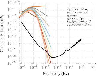
Figure 1: First harmonics of the characteristic amplitude as a function of the frequency for a standard EMRI (see e.g. Amaro-Seoane, 2018b) in the approximation of Peters (1964). We adopt values for the Galactic Centre, so that $M_{\text{BH}}=4.3\times 10^{6}M_{\odot}$ and the distance $D=8\,\text{kpc}$. We consider a one-year duration for the mission. The V-shaped, solid line corresponds to the noise curve $\sqrt{f\,S_{h}(f)}$ for LISA. On the top, right corner we show the initial parameters of the binary which we have considered, which is composed by the massive black hole in our Galaxy, SgrA*, a compact object of mass $m_{*}=10\,M_{\odot}$, with initial semi-major axis $a=10^{-3}\,\text{pc}$ and eccentricity $e=0.997$. Initially, the pericentre of the orbit is located in this approximation at $R_{\text{p}}=7.3\,R_{\text{S}}$, with $R_{\text{S}}$ the Schwarzschild radius of SgrA*. At the beginning of the evolution, the time for the binary to merge due to the emission of gravitational waves is of $T_{\text{mrg}}=7.68\times 10^{4}\,\text{yrs}$.

II.2 Waveforms with extreme eccentricities

Most used EMRI waveforms are based on the work of Peters (1964) and Peters and Mathews (1963), which adopt Keplerian ellipses shriking over time due to the emission of gravitational radiation, as in Eq. (1). Usually it is assumed that a limitation of this derivation is that the eccentricity cannot be arbitrarily large, since the orbit would be like a pulse and non-integrable.

However, EMRIs naturally form via two-body relaxation which leads to extreme eccentricities (see e.g. Amaro Seoane, 2022; Amaro-Seoane, 2018a). It is claimed that none of the existing waveforms can deal with eccentricities typically larger than $e\gtrsim 0.8$, while in the case of EMRIs we are looking at $e\gtrsim 0.99$, in particular if the central supermassive black hole is spinning (Amaro-Seoane et al., 2013), in which case they can achieve higher values. Since a correct calculation of the SNR is important for the problem that we are addressing, in this section we present a way to investigate this apparent problem of extreme eccentricities in an analytical way.

We wish to investigate the behaviour of the solutions to the equations

$$\frac{de}{dt}=-\frac{304e}{15}\frac{G^{3}m_{1}m_{2}(m_{1}+m_{2})}{c^{5}a^{4}(1-e^{2})^{5/2}}\left(1+\frac{121}{304}e^{2}\right),$$ (2)

$$\frac{da}{de}=\frac{12}{19}\frac{a}{e}\frac{\big{[}1+(73/24)e^{2}+(37/96)e^{4}\big{]}}{(1-e^{2})\big{[}1+(121/304)e^{2}\big{]}},$$ (3)

with the initial condition $e(0)\rightarrow 1$, with $e(0)$ the initial eccentricity. For $t$ sufficiently small such that $e(t)$ is close enough to 1, the asymptotic behaviour of these equations is

$$\frac{de}{dt}=-\frac{85}{3}\frac{G^{3}m_{1}m_{2}(m_{1}+m_{2})}{c^{5}}\frac{1}{a^{4}(1-e^{2})^{5/2}},$$ (4)

$$\frac{da}{de}=\frac{2a}{1-e^{2}}.$$ (5)

We start by integrating the second equation.

$$\ln a=\ln\left(\frac{1+e}{1-e}\right)+C,$$ (6)

and therefore

$$a=C\left(\frac{1+e}{1-e}\right).$$ (7)

The integration constant $C$ is fixed by the equation

$$a(0)=C\left(\frac{1+e(0)}{1-e(0)}\right),$$ (8)

with $a(0)$ the initial semi-major axis. Setting $a(0)=a_{0}$ and $e(0)=e_{0}$ gives us

$$a=\underbrace{a_{0}\left(\frac{1-e_{0}}{1+e_{0}}\right)}_{=C}\left(\frac{1+e}{1-e}\right).$$ (9)

We now have to calculate the eccentricity as a function of time. Substituting eq. Eq. (9) to Eq. (4) gives us

$$\frac{de}{dt}=-\frac{1}{\tau}(1-e)^{3/2}(1+e)^{-13/2},$$ (10)

where

$$\frac{1}{\tau}=\frac{85}{3}\frac{G^{3}m_{1}m_{2}(m_{1}+m_{2})}{a_{0}^{4}c^{5}}\left(\frac{1+e_{0}}{1-e_{0}}\right)^{4}.$$ (11)

Again, the equation Eq. (10) is solved by integrating:

$$\int_{e_{0}}^{e}de^{\prime}\,(1-e^{\prime})^{-3/2}(1+e^{\prime})^{13/2}=-\frac{t}{t_{0}}.$$ (12)

The indefinite integral on the left term of the equation above is given by

$$\int de\, (1-e)^{-3/2}(1+e)^{13/2}=\frac{3003}{8}\tan^{-1}\left(\sqrt{\frac{1-e}{1+e}}\right)$$

$$-\frac{\sqrt{e+1}}{240\sqrt{1-e}}\left(40e^{6}+344e^{5}+1406e^{4}\right.$$

$$\left.+3842e^{3}+8933e^{2}+25499e-70784\right).$$ (13)

Thus, in the limit $e\rightarrow 1$ the asymptotic behaviour of the integral is

$$\int_{e_{0}}^{e}de^{\prime}\,(1-e^{\prime})^{-3/2}(1+e^{\prime})^{13/2}=$$

$$128\sqrt{2}\left(\frac{1}{\sqrt{1-e_{0}}}-\frac{1}{\sqrt{1-e}}\right),$$ (14)

giving us the function of the eccentricity as a function of time:

$$e(t)=1-\frac{1-e_{0}}{\left(1+t/t_{0}\right)^{2}},$$ (15)

where

$$t_{0} =\frac{128\sqrt{2}}{\sqrt{1-e_{0}}}\,\tau=$$

$$\frac{384\sqrt{2}}{85}\frac{G^{3}m_{1}m_{2}(m_{1}+m_{2})}{c^{5}}\frac{(1-e_{0})^{7/2}}{a_{0}^{4}(e_{0}+1)^{4}}$$ (16)

The semi-major axis is given by the relation Eq. (9).

In Fig. (2) we show this result for the relationship between the semi-major axis and the eccentricity, and compare it to the numerical integration of the set of equations given by Eq. (3). As we can see, the asymptotic limit describes the numerical result well down to eccentricities of about $e\sim 0.2$ This also confirms that the Peters approximation is a perfectly valid one for eccentricities of up to $e=0.99999$, since it overlaps with the asymptotic solution.

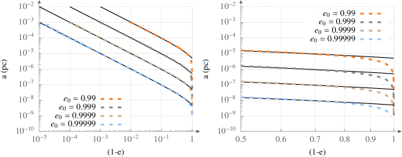
Figure 2: Left panel: Relationship between the semi-major axis and the eccentricity (displayed as $1-e$) as integrated numerically from Eqs. (3), dashed, coloured curves, and the asymptotic solution presented in this section (solid, black lines). We depict different initial eccentricities.

II.3 Signal-to-noise ratio calculation and parameter extraction

The SNR of the n-th harmonic can be approximately calculated using

$$\left(\frac{S}{N}\right)^{2}_{n} \approx\frac{h^{2}_{\rm c,\,n}(f_{n})}{5S_{h}(f_{n})}\frac{\dot{f}_{n}}{f_{n}^{2}}T_{\mathrm{obs}},$$

$$\dot{f}_{n} \approx n\dot{f}_{\mathrm{orb}},$$ (17)

where $T_{\mathrm{obs}}$ is the observation time and $\dot{f}_{\mathrm{orb}}$ is the time derivative of the orbital frequency, which follows from Peters (1964). To be specific, the square of SNR of the n-th harmonic can be written as

$$\left(\frac{S}{N}\right)^{2}_{n} \approx\frac{256}{5}\frac{(G\mathcal{M}_{c})^{10/3}}{c^{8}D^{2}}\frac{g(n,e)}{n^{2}}(2\pi f_{\mathrm{orb}})^{4/3}\times$$

$$\frac{T_{\mathrm{obs}}}{5S_{h}(nf_{\mathrm{orb}})}.$$ (18)

This way we can see the loudness of each harmonic. This approximation is inaccurate when the binary is evolving rapidly, when the timescale is shorter than the observation time. However, since we are focusing on mono- and oligochromatic E-EMRIs in this work, this is not a problem. Polychromatic EMRIs will however need a different treatment.

Therefore, for those cases in which the E-EMRI is close to merger, we generate the corresponding numerical waveforms and obtain the SNR using

$$\left(\frac{S}{N}\right)^{2}=(h|h),$$ (19)

where the inner product of two waveforms $\left(a|b\right)$ is defined in the usual way as

$$\left(a|b\right):=2\int\mathrm{d}f\ \frac{\tilde{a}(f)\tilde{b}^{*}(f)+\tilde{a}^{*}(f)\tilde{b}(f)}{S_{h}(f)}.$$ (20)

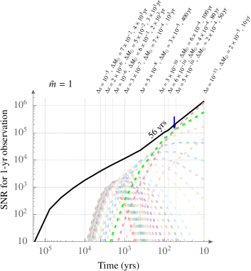
Figure 3: Signal-to-noise calculation for a one-year observation of an E-EMRI at the Galactic Centre with a mass of $\tilde{m}:=1=10\,M_{\odot}$. The solid, black line corresponds to the summation of all individual contributions coming from the different harmonics (dashed, colour curves). The blue arrow shows from which moment the source is circular, i.e. when the second harmonic dominates the contribution to the SNR. The vertical, dotted lines show the times at which the error in the estimation of the spin of the supermassive black hole and its mass, $\Delta s$ and $\Delta M_{\odot}$, respectively, have been calculated. Due to the short distance to the source, which is assumed to be located at the Galactic Centre, the errors are very small, and they become smaller as the source evolves with time.

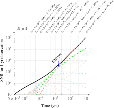
Figure 4: Same as Fig. (3) but for a mass of $\tilde{m}:=4=40\,M_{\odot}$.

A full comparison between the SNRs obtained in different approach can be found in Table 1.

$T_{\mathrm{mrg}}$ (yr)	$n$	$\mathrm{SNR_{0}}$	$\mathrm{SNR_{aprx}}$	$\mathrm{SNR^{\prime}_{aprx}}$	$\mathrm{SNR_{LW}}$
10	$1-10$	$1.45\times 10^{6}$	$4.99\times 10^{5}$	$4.99\times 10^{5}$	$3.66\times 10^{5}$
50	$1-10$	$2.27\times 10^{5}$	$1.24\times 10^{5}$	$1.24\times 10^{5}$	$1.25\times 10^{5}$
80	$1-10$	$1.24\times 10^{5}$	$7.75\times 10^{4}$	$7.75\times 10^{4}$	$8.55\times 10^{4}$
100	$1-10$	$1.05\times 10^{5}$	$6.85\times 10^{4}$	$6.85\times 10^{4}$	$7.65\times 10^{4}$
400	$1-30$	$2.71\times 10^{4}$	$2.32\times 10^{4}$	$2.32\times 10^{4}$	$2.89\times 10^{4}$
2000	$9-38$	$7.16\times 10^{3}$	$6.93\times 10^{3}$	$7.10\times 10^{3}$	$9.57\times 10^{3}$
3000	$19-48$	$4.63\times 10^{3}$	$4.62\times 10^{3}$	$5.17\times 10^{3}$	$7.04\times 10^{3}$
4000	$31-60$	$3.06\times 10^{3}$	$3.08\times 10^{3}$	$3.88\times 10^{3}$	$5.36\times 10^{3}$

Table 1: The SNRs calculated in different approaches. The first column shows the merger time of the system in years and the second the harmonic number. The 3rd column ’$\mathrm{SNR_{0}}$’ is calculated by generating the waveforms and taking the square-root of the inner product of the waveform and itself. The Waveforms are generated with the 10 or 30 loudest harmonics, which are given in the 2nd column ’n’. The 4th column ’$\mathrm{SNR_{aprx}}$’ is calculated using the approximation given in 17 and considering only the 10 or 30 loudest harmonics given in the 2nd column. The 5th column ’$\mathrm{SNR^{\prime}_{aprx}}$’ uses the same approximation but consider the first 10000 harmonics. The 6th column ’$\mathrm{SNR_{LW}}$’ is calculated using the python package LEGWORK(Wagg et al., 2022).

Fig. (3) shows the contribution of the first 30 harmonics of an E-EMRI with a mass of $10\ M_{\odot}$, and Fig. (4) for an E-EMRI of mass $40\ M_{\odot}$. The SNRs are calculated using Equation (17), while the SNRs of the cases $\leq 100$ yr are calculated using Equation (19).

	$T_{\mathrm{mrg}}(\mathrm{yr})$	$R_{\mathrm{p}}(R_{\mathrm{S}})$	$e$	$a(\mathrm{pc})$
in-band	$1.85\times 10^{5}$	7.31	0.999333	$4.52\times 10^{-3}$
threshold	$56$	4.08	0.2244	$2.17\times 10^{-6}$

Table 2: Time before merger ($T_{\mathrm{mrg}}$) in years, pericentre distance in Schwarzschild radii units ($R_{\mathrm{p}}$), eccentricity and semi-major axis in pc of an E-EMRI with a mass of $10\ M_{\odot}$ at two specific moments: (1) in-band, the moment when the SNR of this system reaches 10; (2) threshold, the moment from which the source becomes circular, i.e. the second harmonic dominates. These data are used later for the calculation of number of sources in band when they are eccentric and circular.

	$T_{\mathrm{mrg}}(\mathrm{yr})$	$R_{\mathrm{p}}(R_{\mathrm{S}})$	$e$	$a(\mathrm{pc})$
in-band	$5\times 10^{5}$	23.93	0.959765	$2.45\times 10^{-4}$
threshold	$650$	11.47	0.1541	$5.59\times 10^{-6}$

Table 3: Same as Table (2) but for a mass of $40\,M_{\odot}$.

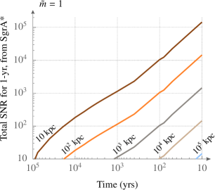
Figure 5: SNR for sources located at different distances from our Galaxy, assuming a one-year observation time. We can see that LISA can in principle observe E-EMRIs (of mass $10\,M_{\odot}$) in galaxies out to distance of approximately 0.1 Gpc.

We perform a Fisher matrix analysis to see how precise we can measure the mass and the spin of the SMBH with a single event. The results at different time are listed in Table (4) for the $10\,M_{\odot}$ source and Table (5) for the $40\,M_{\odot}$ one. The analysis is carried out numerically and requires generation of the numerical waveforms of. The generation of such waveforms can be time-consuming when the eccentricity of the orbit is very large, since more harmonics contribute and must hence be calculated. Due to limited computation time, we have only calculated those cases close to merger (with low eccentricity). The case with the lowest orbital frequency in both tables is the last line in Table 5 (corresponding to $40\ M_{\odot}$ and $4\times 10^{4}$ years before plunge), in which the compact object can still make $>100$ orbits in 1-yr observation time and thus guarantees the reliability of the Fisher matrix analysis.

$T_{\mathrm{mrg}}$ ($\mathrm{yr}$)	$e$	$R_{\mathrm{p}}^{\,0}(R_{\mathrm{S}})$	$n$	$\Delta$ s	$\Delta M$ ($M_{\odot}$)
10	0.1216	3.0	$1-10$	$1\times 10^{-11}$	$2\times 10^{-5}$
50	0.21515	4.0	$1-10$	$5\times 10^{-10}$	$2\times 10^{-4}$
80	0.25489	4.4	$1-10$	$6\times 10^{-10}$	$4\times 10^{-4}$
100	0.27592	4.5	$1-10$	$3\times 10^{-10}$	$6\times 10^{-4}$
400	0.45551	5.5	$1-30$	$5\times 10^{-8}$	$3\times 10^{-5}$
1000	0.60832	6.2	$3-32$	$3\times 10^{-7}$	$7\times 10^{-4}$
2000	0.72767	6.5	$9-38$	$1\times 10^{-6}$	$6\times 10^{-3}$
3000	0.79255	6.7	$19-48$	$2\times 10^{-6}$	$5\times 10^{-2}$
4000	0.83423	6.9	$31-60$	$1\times 10^{-5}$	$7\times 10^{-2}$

Table 4: Parameter extraction via Fisher matrix analysis of an E-EMRI with a mass of $10\ M_{\odot}$. From the left to the right we show the time for merger in years, the eccentricity, the initial periapsis distance, the loudest harmonics used in the generation of the waveforms, the error in the spin measurement and the error in the measurement of the mass of the MBH, SgrA*.

$T_{\mathrm{mrg}}$ ($\mathrm{yr}$)	$e$	$R_{\mathrm{p}}^{\,0}(R_{\mathrm{S}})$	$n$	$\Delta$ s	$\Delta M$ ($M_{\odot}$)
10	0.029	4.5	$1-10$	$5\times 10^{-11}$	$9\times 10^{-10}$
30	0.046	5.9	$1-10$	$4\times 10^{-10}$	$3\times 10^{-4}$
100	0.074	7.7	$1-10$	$1\times 10^{-9}$	$2\times 10^{-4}$
400	0.130	10.5	$1-10$	$5\times 10^{-7}$	$9\times 10^{-4}$
1000	0.180	12.4	$1-10$	$2\times 10^{-6}$	$1\times 10^{-1}$
2000	0.237	14.1	$1-15$	$7\times 10^{-6}$	$2\times 10^{-1}$
4000	0.311	15.9	$1-15$	$5\times 10^{-6}$	$5\times 10^{-1}$
$1\times 10^{4}$	0.430	18.1	$1-20$	$2\times 10^{-4}$	$2$
$2\times 10^{4}$	0.538	19.7	$1-30$	$6\times 10^{-4}$	$1$
$4\times 10^{4}$	0.692	21.4	$8-37$	$4\times 10^{-3}$	$7$

Table 5: Same as Table (4) but for a mass of $40\ M_{\odot}$

III Number of E-EMRIs in band at the Galactic Centre

In order to calculate the number of these sources in band, we adopt the result of Amaro-Seoane (2019), which can be directly applied to our problem. In his work, the author derives the event rate ${\Gamma}$ for merging stellar-mass black holes with supermassive black holes as a test in his Eq. (40),

$${\Gamma} \sim 1.92\times 10^{-6}\,\textrm{yrs}^{-1}\tilde{N}_{0}\,\tilde{\Lambda}\,\tilde{R}_{0}^{-2}\,\tilde{m}^{2}\times$$

$$\Bigg{\{}1.6\times 10^{-1}\tilde{R}_{0}^{1/2}\tilde{N}_{0}^{-1/2}\tilde{\Lambda}^{-1/2}\tilde{m}^{1/2}\,{\cal W}(\iota,\,{\rm s})^{-5/4}\times$$

$$\left[\ln\left(9138\,\tilde{R}_{0}\,\tilde{N}_{0}^{-1}\tilde{\Lambda}^{-1}\tilde{m}\,{\cal W}(\iota,\,{\rm s})^{-5/2}\right)-2\right]-$$

$$4\times 10^{-2}\tilde{R}_{0}^{1/2}\times\left[\ln\left(618\,\tilde{R}_{0}\right)-2\right]\Bigg{\}},$$ (21)

with the following notation,

$$\tilde{\Lambda} :=\left(\frac{\ln(\Lambda)}{13}\right),~{}\tilde{N}_{0}:=\left(\frac{N_{0}}{12000}\right)$$

$$\tilde{R}_{0} :=\left(\frac{R_{\rm h}}{1\textrm{pc}}\right),~{}\tilde{m}:=\left(\frac{m}{10\,M_{\odot}}\right).$$ (22)

Here $\ln(\Lambda)\simeq\ln(M_{\rm BH}/m)$, with $M_{\rm BH}$ the mass of the MBH, $m$ the mass of the stellar-mass black hole (see Amaro-Seoane, 2018a) and $N_{0}$ the number of stellar-mass black holes within a radius $R_{0}$ where relaxation can be enviaged to be completely dominated by this kind of compact objects. In the same work, Amaro-Seoane (2019) explains why $R_{0}$ should be set to the influence radius $R_{\rm h}$ (which we accordingly use in the numerator of the equation). The function $\cal{W}(\iota,\,{\rm s})$ reflects the location of the separatrix of a Kerr MBH as compared to a Schwarzschild case, and depends on the magnitude of the spin of the MBH, $\rm{s}$ and the inclination of the orbit, $\iota$ (Amaro-Seoane et al., 2013).

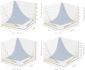
Figure 6: Upper panels: Event rates, i.e. mergers, as derived in Eq. (21) for a stellar-mass black hole of mass $\tilde{m}=1$, which corresponds to $10\,M_{\odot}$ for an influence radius of 3pc (left panel) and 1 pc (right panel). We depict the rates as a function of the value of the spin of the supermassive black hole, whose mass is set to $4.3\times 10^{6}\,M_{\odot}$ and the inclination of the orbit in radians. Lower panels: Same but for a mass of $40\,M_{\odot}$.

We note that Eq. (21) is self-contained. This means that it contains the information about the integration limits to derive the event rates; i.e. the number of stellar-mass black holes plunging through the event horizon of the MBH per year. These two limits are the minimum radius, the distance within which we expect to have at least one object to start the integration, and the threshold radius which divides the relaxation-dominated regime and the one in which the driving mechanism is the emission of gravitational waves (see Amaro-Seoane, 2019, 2018a, for a more detailed explanation and derivation). This radius is given in Eq.(28) of Amaro-Seoane (2019) in a general expression. In the particular case of a stellar-mass black hole, this radius is

$$a_{\rm crit} =R_{0}\Bigg{[}\frac{20480}{1207}(3-\gamma)(1+\gamma)^{3/2}\times$$

$$\times C\,{\cal W}(\iota,\,{\rm s})^{5/2}\,N_{0}\ln(\Lambda)\left(\frac{M_{\rm BH}}{m}\right)^{-1}\Bigg{]}^{\frac{1}{\gamma-3}},$$ (23)

where $C$ is a factor of order 1 and $\gamma$ is the exponential of the power-law cusp that the stellar-mass black holes form around the MBH. For an initial-mass function which represents our Galaxy, this is $\gamma=2$ (Preto and Amaro-Seoane, 2010; Alexander and Hopman, 2009).

Hence, we can use Eq. (21) for any mass of stellar-mass black hole that we want to address. We only need to choose the mass of the object, since $\tilde{\Lambda}$ and $\tilde{N_{0}}$ are the same for all masses. With the choice of the mass, the rest of the parameters is accordingly fixed.

In order to obtain the number of sources in band, we follow exactly the same argument we introduced in Amaro-Seoane (2019), and we therefore refer the reader to that work for details. Although in that work we were focusing on a different kind of source, the physical idea remains the same. We succinctly summarise the fundamentals. One could think that the total number of sources in band can be obtained by simply multiplying the event rate by the time spent in band. The total number of sources that the observatory is to detect can be derived by solving a differential equation. We know the influx of new sources from the stellar system thanks to relaxation theory, which allows us to define the critical radius which we presented before, and we know how often one of them disappears from the system through the sink, since we have the rates, i.e. how often it merges with the central MBH. By multiplying the number of sources per year by the time spent on band, we should obtain the number of sources at any given time.

This argument is however not correct, since the energy of the E-EMRIs sources must be below a threshold value in phase-space, as specified in Amaro-Seoane (2019). It is not enough to diffuse in energy to achieve semi-major axis values below $a_{\text{crit}}$ as given by Eq. (23). We recall that $a_{\text{crit}}$ merely marks the transition in the value of the semi-major axis from the regime in which dynamics dominates the evolution of the binary to the one dominated by general relativity (see Fig. 5 of Amaro-Seoane (2019)). From that value, the binary still has a long way to do until it enters the band of the detector. I.e. the orbital period must become much shorter. Not all sources crossing the critical radius will successfully arrive to that point.

Therefore, E-EMRIs approach must first shrink their semi-major axes to values lower than $a_{\text{crit}}$, and only a fraction of them will arrive to a value which we call $a_{\text{band}}$, in which the source is in band. From there they will slowly circularise and cross $a_{\text{thr}}$ to finally cross the minimum semi-major axis which leads to a merger, $a_{\text{min}}$.

In physical space, finding which sources do arrive corresponds to solving in the limit in which $\Delta t\to 0$ the following continuity equation for a line density function $l\equiv dN/da$ with $N$ the number of sources with a given energy

$$\frac{\partial}{\partial a}\Big{[}\,\dot{a}(a,\,e)\,l\,\Big{]}+\frac{\partial l}{\partial t}=0.$$ (24)

Following Amaro-Seoane (2019), we now introduce two different regimes, which will allow us to normalise $N$ and obtain the total number of sources. We thus distinguish the circular and the eccentric regime and a threshold distance $a_{\rm thr}$ which marks that transition. In the eccentric regime, we will approximate the eccentricity to be $e\sim 1$ and vice-versa, in the circular regime we will take $e\sim 0$. In practice, $a_{\rm thr}$ can be determined by finding out when the second harmonic dominates over the rest of them. We have this information from the previous section. We can take a representative case, for instance that of Fig. (1), in which this transition happens at a pericentre distance of $R_{\text{p}}=3.67\,R_{\text{S}}$ and an eccentricity of $e\sim 0.18$. Therefore we have that $a_{\rm thr}=R_{\text{p}}/(1-e)\sim 4.5\,R_{\text{S}}\sim 2\times 10^{-6}\,\text{pc}$, since for $M_{\text{BH}}=4.3\times 10^{6}\,M_{\odot}$, we have $R_{\text{S}}\sim 4\times 10^{-7}\,\text{pc}$. On the other hand, the minimum semi-major axis can be defined to be $a_{\text{min}}=2\times R_{\text{S}}\sim 8\times 10^{-7}\,\text{pc}$.

Let us call the number of sources comprised between $a_{\text{min}}$ and $a_{\text{thr}}$, $N_{\text{I}}$, the number comprised between $a_{\text{thr}}$ and $a_{\text{band}}$, $N_{\text{II}}$ and from there to $a_{\text{crit}}$, $N_{\text{III}}$ (as in Fig. 7 of Amaro-Seoane (2019)). From the same work, the solution to the differential equation is

$$\frac{N_{\rm II}}{N_{\rm III}} =\frac{a_{\rm band}^{1/2}-a_{\rm thr}^{1/2}}{a_{\rm crit}^{1/2}-a_{\rm band}^{1/2}}$$

$$\frac{N_{\rm I}}{N_{\rm II}+N_{\rm III}} =\frac{1}{8}\times\frac{1-\left(a_{\rm min}/a_{\rm thr}\right)^{4}}{\left(a_{\rm crit}/a_{\rm thr}\right)^{1/2}-1}$$

$$N_{\rm I}+N_{\rm II} ={\Gamma}\times T\left(a,\,e\right),$$ (25)

with $T\left(a,\,e\right)$ the amount of time spent on band with a minimum SNR of 10.

Therefore, the full expression for each number of E-EMRIs per interval is given by the expressions

$$N_{\rm I} =\frac{CD(1+A)}{A+(1+A)D}$$

$$N_{\rm II} =\frac{CA}{A+(1+A)D}$$

$$N_{\rm III} =\frac{C}{A+(1+A)D},$$ (26)

with

$$A \equiv\frac{a_{\rm band}^{1/2}-a_{\rm thr}^{1/2}}{a_{\rm crit}^{1/2}-a_{\rm band}^{1/2}}$$

$$D \equiv\frac{1}{8}\frac{1-\left(a_{\rm min}/a_{\rm thr}\right)^{4}}{\left(a_{\rm crit}/a_{\rm thr}\right)^{1/2}-1}$$

$$C \equiv{\Gamma}\times T\left(a,\,e\right).$$ (27)

More explicitly,

$$N_{\rm I} ={\Gamma}\times T\left(a,\,e\right)\times\Omega_{1}$$

$$N_{\rm II} ={\Gamma}\times T\left(a,\,e\right)\times\Omega_{2}$$

$$N_{\rm III} ={\Gamma}\times T\left(a,\,e\right)\times\Omega_{3},$$ (28)

where we have introduced the weighting functions $\Omega_{1}$, $\Omega_{2}$ and $\Omega_{3}$ given in Eqs. (29)

$$\Omega_{1} \equiv\frac{(\sqrt{a_{\rm thr}}-\sqrt{a_{\rm crit}})(a_{\rm min}^{4}-a_{\rm thr}^{4})}{(a_{\rm thr}^{4}(8\sqrt{a}(\sqrt{a_{\rm crit}/a_{\rm thr}}-1)+\sqrt{a_{\rm crit}})+a_{\rm thr}^{9/2}(7-8\sqrt{a_{\rm crit}/a_{\rm thr}})+a_{\rm min}^{4}(\sqrt{a_{\rm thr}}-\sqrt{a_{\rm crit}})}$$

$$\Omega_{2} \equiv\frac{8a_{\rm thr}^{4}(\sqrt{a}-\sqrt{a_{\rm thr}})(\sqrt{a_{\rm crit}/a_{\rm thr}}-1)}{a_{\rm thr}^{4}(8\sqrt{a}(\sqrt{a_{\rm crit}/a_{\rm thr}}-1)+\sqrt{a_{\rm crit}})+a_{\rm thr}^{9/2}(7-8\sqrt{a_{\rm crit}/a_{\rm thr}})+a_{\rm min}^{4}(\sqrt{a_{\rm thr}}-\sqrt{a_{\rm crit}})}$$

$$\Omega_{3} \equiv\frac{8a_{\rm thr}^{4}(\sqrt{a}-\sqrt{a_{\rm crit}})(1-\sqrt{a_{\rm crit}/a_{\rm thr}})}{(a_{\rm thr}^{4}(8\sqrt{a}(\sqrt{a_{\rm crit}/a_{\rm thr}}-1)+\sqrt{a_{\rm crit}})+a_{\rm thr}^{9/2}(7-8\sqrt{a_{\rm crit}/a_{\rm thr}})+a_{\rm min}^{4}(\sqrt{a_{\rm thr}}-\sqrt{a_{\rm crit}})}$$ (29)

In Fig. (7) we display the result for a stellar-mass black hole of mass $10\,M_{\odot}$ and different influence radii. The value of this parameter has an important impact in the total number of E-EMRIs in the three different regions, as we can see. Observations of the Galactic Centre derive a value of $R_{\text{infl}}=3\,\text{pc}$ Schödel et al. (2018), but we also add the results for $R_{\text{infl}}=1\,\text{pc}$, which has been the “default” value in the related literature. The number of E-EMRIs in the oligochromatic phase, i.e. in the range of frequencies close to that of a polychromatic EMRI, are negligible, of the order of $10^{-3}$ for both values of the influence radius. As we move to lower frequencies and get into the monochromatic stage, we can expect to have two sources if the influence radius is one, with associated SNR values around $10^{5}$, as we can see in Fig. (3). In the farthest region, where the sources are more eccentric, the number of E-EMRIs lies between 8 and 20, with SNRs that are smaller in comparison but still around thousands.

We also show the results for a different mass value of the stellar-mass black hole, $40\,M_{\odot}$, and different influence radii, in Fig. (8). In this case, and as we expected from the larger event rates and time spent on band, the numbers are more interesting. In region $N_{\text{I}}$, where we can expect E-EMRIs to get SNR values close to $10^{6}$, as we can see in Fig. (4), we expect to have between one or a handful of sources, depending on the value of $R_{\text{infl}}=3\,\text{pc}$. In region $N_{\text{II}}$, the numbers range between 45 and 200, and the SNR is typically of the order $10^{4}$. Finally, in region $N_{\text{I}}$, where the SNR is the lowest, but still can reach values as high as thousands, we predict between 2000 and 5000 sources.

It is important to stress out that these numbers are not to be envisaged as rates of stellar-mass black holes crossing the event horizon. They are telling us how many E-EMRIs are at the Galactic Centre as the result of a steady-state analysis. I.e. they represent on average the number of E-EMRIs which can be found in galactic nuclei (with the representative parameters we have addressed) at any given moment in the evolution of that nucleus. The proviso is that the nucleus is relaxed, which is true if the mass of the MBH has at most a few times $10^{7}\,M_{\odot}$ Amaro Seoane (2022), but also that the MBH is fixed at the centre of the system: for intermediate-mass black holes the derivation would be significantly more complex, since it would be wandering around the centre.

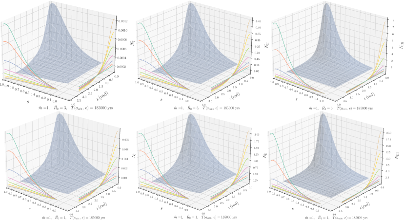
Figure 7: Number of E-EMRIs $N({\rm s},\,\iota)$ as a function of the inclination of the orbit $\iota$ and the spin of the MBH, s, for a stellar-mass black hole of mass $10\,M_{\odot}$ and two influence radii, 3pc (upper panels) and 1pc (lower panels). From the left to the right we have the number of sources for the regions $N_{\rm I}$, $N_{\rm II}$ and $N_{\rm III}$.

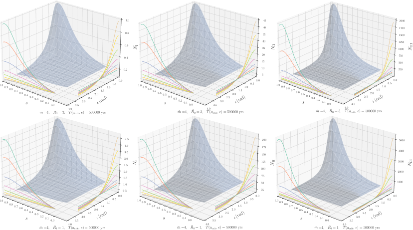
Figure 8: Same as Fig. (7) but for a stellar-mass black hole of mass $40\,M_{\odot}$.

IV A forest of E-EMRIs

In this section we estimate what the foreground signal of continuous E-EMRIs would be. There are two important assumptions we are making. First, the binning in frequencies is broader than what in reality LISA will be. This is so because the computational estimation of thinner binnings is too demanding. The implication is that we are assuming that the sources are contributing in an incoherent way. As mentioned in the introduction, this is not necessarily the case: A narrower binning might allow us to distinguish individual sources, in particular when they are far away from their polychromatic behaviour, i.e. when they are “monochromatic”. The second one is that we consider only continuous signals, and hence from the thousands mentioned previously we are left with only about 160 of them for the $10\,M_{\odot}$, as we explain later. In reality, however, there will be sources contributing to the signal which are not continuous. However, discontinuous sources can be dealt with, as we mention later.

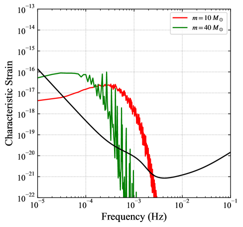
Figure 9: Total contribution of of E-EMRIs at the Galactic Centre during 1-yr observation time. The two different colours indicates different masses of the E-EMRIs, assumed to be of either $10\,M_{\odot}$ or $40\,M_{\odot}$. As we move towards higher frequencies, the signal becomes less smooth because there are less and less individual sources. On the other hand, the closer to merger, the larger the SNR, which explains why the characteristic amplitude does not drop as quick as one would naively expect.

The characteristic strain of the E-EMRI background $h_{c,\mathrm{gwb}}$ can be calculated using the following expression

$$h^{2}_{c,\mathrm{gwb}}(f)=\frac{1}{2} \int\mathrm{d}\mathcal{M}\ \mathrm{d}e\left[\sum_{n}\frac{\mathrm{d}^{4}N}{\mathrm{d}\mathcal{M}\ \mathrm{d}e\ \mathrm{d}\ln{f_{\mathrm{orb}}}}\times\frac{h_{c,n}^{2}}{fT_{\mathrm{obs}}}\right],$$ (30)

$$f_{\mathrm{orb}} =\frac{f(1+z)}{n}\in[f_{\mathrm{orb,min}},f_{\mathrm{orb,max}}],$$

where we have followed the same nomenclature as in (Bonetti and Sesana, 2020); i.e. $\mathcal{M}$ is the the source-frame chirp mass, $f_{\mathrm{orb,min}}$ and $f_{\mathrm{orb,max}}$ are the minimum and maximum orbital frequencies and $z$ the redshift (which in our case is zero, since we are focusing on the Galactic Centre).

We depict the result in Fig. (9). The orbital parameters (eccentricity and orbital frequency) of these E-EMRIs are selected as follows: (1) We pick an E-EMRI that has just entered the LISA band; (2) we then evolve it until 1 year before plunge (the assumed observational time); (3) we randomly choose different instants from the above evolution process, which allows us to interpret them as different E-EMRIs instead of calculating different waveforms for each source; finally, (4) we calculate their characteristic strain and sum them up. We do such calculations both for the mass of the stellar-mass black hole $m=10~{}M_{\odot}$ and $m=40~{}M_{\odot}$ (shown as red and green line in Figure 9). The mass of the MBH is fixed to $M_{\mathrm{BH}}=4.3\times 10^{6}\ M_{\odot}$. The initial parameters are $e=0.983005,~{}a=1.76376\times 10^{-4}~{}\rm pc$ for $m=10~{}M_{\odot}$ and $e=0.959765,~{}a=2.45\times 10^{-4}~{}\rm pc$ for $m=40~{}M_{\odot}$.

The initial parameters above correspond to the in-band parameters in Tables (2) and (3). We note that in the $10~{}M_{\odot}$ case we adopt the parameters of an E-EMRI $3.03\times 10^{4}~{}\rm yr$ before plunge. From the total initial number we select only continuous E-EMRIs, which decreases the total number to $\sim 163$ in the $10\,M_{\odot}$. As mentioned before, this is due to limited computation time, since E-EMRIs at their early age have smaller orbital frequency and large eccentricity, and therefore require more harmonics to be considered in the calculation, which causes the computation time to grow rapidly. In the $40\,M_{\odot}$ case, all of the initial cases were kept, i.e. they were continuous.

The LISA band is divided into bins of width $\delta f\sim 10^{-5}\ \mathrm{Hz}$). For each E-EMRI in the sample, we calculate the characteristic strain of all the harmonics in LISA band ($10^{-5}\ \mathrm{Hz}<nf_{\mathrm{orb}}<10^{-1}\ \mathrm{Hz}$) and add their contribution to the corresponding bins. The contribution of the $n$-th harmonic of the $m$-th E-EMRI $(h^{2}_{c,\mathrm{gwb}})_{m,n}$ is calculated with

$$(h^{2}_{c,\mathrm{gwb}})_{m,n}=\left\{\begin{aligned} &\frac{h^{2}_{c,n}}{2fT_{\mathrm{obs}}}\quad&\mathrm{if}\ \Delta f_{m,n}>\delta f\\ &\frac{fh^{2}_{n}}{2\ \delta f}&\mathrm{if}\ \Delta f_{m,n}\leq\delta f,\end{aligned}\right.$$ (31)

where $f=nf_{\mathrm{orb},m}$ is the frequency of this harmonic and $\Delta f_{m,n}$ is the change of the frequency during the observation time of $T_{\mathrm{obs}}=1~{}\mathrm{yr}$. If $\Delta f_{m,n}>\delta f$, we would assume that this harmonic affects more than one frequency bin, and contributes noise to all the bins related. Otherwise, its contribution is limited to only one bin. We repeat the above procedure five times and average the results to ensure the statistical reliability.

V Conclusions

In this work we have estimated the number of sources which are on their way to becoming EMRIs at our Galactic Centre. The number of them crossing the event horizon, i.e. the mergers, is very low, as expected. However, we show that at any given time (meaning that this is a steady-state solution, with the proviso that the relaxation time is shorter than the Hubble time and the MBH is fixed at the centre) there is a large number of early-stage EMRIs (which we dub E-EMRIs), i.e. EMRIs which yield a SNR of at least 10 in the LISA observatory for a one year observation time. The interesting feature is that E-EMRIs can spend up to $5\times 10^{5}$ years in band with a SNR starting at 10.

Using waveforms following the scheme of (Barack and Cutler, 2004a, b), we perform a SNR calculation and a Fisher matrix study in order to extract parameters. We also perform an asymptotic analysis of the equations when $e\to 1$ and find that the treatment of the eccentricity for extreme values is correct.

Due to the short distance to the Galactic Centre, we find SNR ranging between a minimum of 10 to up to $10^{6}$ depending on their evolutionary stage. Because of the large SNRs, E-EMRIs can be detected in other galaxies, out to 0.1 Gpc. In our parameter study we focus on the spin and mass of the MBH of our Galactic Centre and find errors as small as $10^{-11}$ and $10^{-5}\,M_{\odot}$ respectively.

We distinguish three different kinds of E-EMRIs depending on their evolutionary phases so as to derive the number of them based on a normalisation of their orbital parameters by integrating a line density function. We focus on two different kind of masses in this work, $40\,M_{\odot}$ and $10\,M_{\odot}$ (but obviously the spectrum will not have only two components in nature). We find that there can be as many as thousands (tens, in the $10\,M_{\odot}$ case) when they are in their very early phase (i.e. when they are the farthest from merger but with a SNR of at least 10), hundreds (a few, in the $10\,M_{\odot}$ case) later, when they have lost a significant amount of their eccentricity, and a few (basically zero for the $10\,M_{\odot}$ case) when they have circularised.

Considering only continuous sources, we estimate the incoherent sum of the individual contributions of E-EMRIs and find that their signal will reach values as high as $10^{-16}$ in characteristic amplitude and as far as $3\times 10^{-2}$ Hz in frequency. However, because of the computational time, we have used a binning in frequency which is larger than we expect to have with LISA. Indeed, depending on the mission duration, the binning will allow us to discern some individual sources, which would have interesting implications due to the large SNRs, as explained before.

This might pose a problem for polychromatic EMRIs, “the ones we have been talking about all along” in the literature (to use Bernard Schutz’ words), because they might be partially or even completely buried in the signal created by E-EMRIs. The problem becomes even harder when considering the white dwarf confusion signal.

As a final note, the sources we have addressed when calculating the total signal have at least a full period for this treatment, i.e. we have considered sources with $P_{\rm orb}\leq T_{\rm obs}$ because otherwise the Fourier treatment would be ill-defined. The rest of the sources will contribute in a different manner. Very eccentric sources only emit radiation when they are close to pericentre i.e. over a short time span $dt_{\rm peri}$ which is very short compared to the orbital period. In principle one could take $dt_{\rm peri}\sim R_{\rm peri}/V_{\rm peri}$, where $R_{\rm peri}$ is the periapsis distance and $V_{\rm peri}$ the associated velocity. The probability that such a source passes pericentre while LISA is operating is then simply $P_{\rm orb}/T_{\rm obs}$ independently of $dt_{\rm peri}$ as long as $dt_{\rm peri}\ll T_{\rm obs}$, which is the condition for the source to be considered as a short burst, a “pop”. We dub this kind of sources “popcorn EMRIs” and note that even though they are not continuous signals, one can still Fourier transform them using the family of all smooth (i.e. infinitely differentiable) functions $f$ on $\mathbf{R}$ that vanish faster than any polynomial, the Schwarz space. This will be presented elsewhere in a separate work.

References

- Einstein (1916) A. Einstein, Sitzungsberichte der Königlich Preußischen Akademie der Wissenschaften (Berlin , 688 (1916).
- Einstein (1918) A. Einstein, Sitzungsberichte der Königlich Preußischen Akademie der Wissenschaften (Berlin , 154 (1918).
- Amaro-Seoane (2018a) P. Amaro-Seoane, Living Reviews in Relativity 21, 4 (2018a), arXiv:1205.5240 .
- Amaro Seoane (2022) P. Amaro Seoane, in Handbook of Gravitational Wave Astronomy. Edited by C. Bambi (2022) p. 17.
- Amaro-Seoane et al. (2007) P. Amaro-Seoane, J. R. Gair, M. Freitag, M. C. Miller, I. Mandel, C. J. Cutler, and S. Babak, Classical and Quantum Gravity 24, 113 (2007), arXiv:astro-ph/0703495 .
- Amaro-Seoane et al. (2017) P. Amaro-Seoane, H. Audley, S. Babak, J. Baker, E. Barausse, P. Bender, E. Berti, P. Binetruy, M. Born, D. Bortoluzzi, J. Camp, C. Caprini, V. Cardoso, M. Colpi, J. Conklin, N. Cornish, C. Cutler, K. Danzmann, R. Dolesi, L. Ferraioli, V. Ferroni, E. Fitzsimons, J. Gair, L. Gesa Bote, D. Giardini, F. Gibert, C. Grimani, H. Halloin, G. Heinzel, T. Hertog, M. Hewitson, K. Holley-Bockelmann, D. Hollington, M. Hueller, H. Inchauspe, P. Jetzer, N. Karnesis, C. Killow, A. Klein, B. Klipstein, N. Korsakova, S. L. Larson, J. Livas, I. Lloro, N. Man, D. Mance, J. Martino, I. Mateos, K. McKenzie, S. T. McWilliams, C. Miller, G. Mueller, G. Nardini, G. Nelemans, M. Nofrarias, A. Petiteau, P. Pivato, E. Plagnol, E. Porter, J. Reiche, D. Robertson, N. Robertson, E. Rossi, G. Russano, B. Schutz, A. Sesana, D. Shoemaker, J. Slutsky, C. F. Sopuerta, T. Sumner, N. Tamanini, I. Thorpe, M. Troebs, M. Vallisneri, A. Vecchio, D. Vetrugno, S. Vitale, M. Volonteri, G. Wanner, H. Ward, P. Wass, W. Weber, J. Ziemer, and P. Zweifel, ArXiv e-prints (2017), arXiv:1702.00786 [astro-ph.IM] .
- Amaro-Seoane et al. (2015) P. Amaro-Seoane, J. R. Gair, A. Pound, S. A. Hughes, and C. F. Sopuerta, Journal of Physics Conference Series 610, 012002 (2015), arXiv:1410.0958 .
- Peters (1964) P. C. Peters, Physical Review 136, 1224 (1964).
- Maggiore (2018) M. Maggiore, Gravitational Waves: Volume 2: Astrophysics and Cosmology, Gravitational Waves (Oxford University Press, 2018).
- Maggiore (2008) M. Maggiore, Gravitational Waves: Volume 1: Theory and Experiments, Gravitational Waves (OUP Oxford, 2008).
- Amaro-Seoane (2019) P. Amaro-Seoane, Phys.Rev.D. 99, 123025 (2019), arXiv:1903.10871 [astro-ph.GA] .
- Barack and Cutler (2004a) L. Barack and C. Cutler, Phys. Rev. D 69, 082005 (2004a), gr-qc/0310125 .
- Barack and Cutler (2004b) L. Barack and C. Cutler, Phys. Rev. D 70, 122002 (2004b), arXiv:gr-qc/0409010 [gr-qc] .
- Finn and Thorne (2000) L. S. Finn and K. S. Thorne, Phys. Rev. D 62, 124021 (2000), gr-qc/0007074 .
- Amaro-Seoane (2018b) P. Amaro-Seoane, Living Reviews in Relativity 21, 4 (2018b).
- Peters and Mathews (1963) P. C. Peters and J. Mathews, Physical Review 131, 435 (1963).
- Amaro-Seoane et al. (2013) P. Amaro-Seoane, C. F. Sopuerta, and M. D. Freitag, MNRAS 429, 3155 (2013), arXiv:1205.4713 [astro-ph.CO] .
- Wagg et al. (2022) T. Wagg, K. Breivik, and S. E. de Mink, 260, 52 (2022), arXiv:2111.08717 [astro-ph.HE] .
- Preto and Amaro-Seoane (2010) M. Preto and P. Amaro-Seoane, ApJ Lett. 708, L42 (2010), arXiv:0910.3206 .
- Alexander and Hopman (2009) T. Alexander and C. Hopman, ApJ 697, 1861 (2009).
- Schödel et al. (2018) R. Schödel, E. Gallego-Cano, H. Dong, F. Nogueras-Lara, A. T. Gallego-Calvente, P. Amaro-Seoane, and H. Baumgardt, A&A 609, A27 (2018), arXiv:1701.03817 .
- Bonetti and Sesana (2020) M. Bonetti and A. Sesana, Phys. Rev. D 102, 103023 (2020), arXiv:2007.14403 [astro-ph.GA] .