Entrywise tensor-train approximation of large tensors via random embeddings

Abstract

The theory of low-rank tensor-train approximation is well-understood when the approximation error is measured in the Frobenius norm. The entrywise maximum norm is equally important but is significantly weaker for large tensors, making the estimates obtained via the Frobenius norm and norm equivalence pessimistic or even meaningless. In this article, we derive a new, direct estimate of the entrywise approximation error that is applicable in such cases. Our argument is based on random embeddings, the tensor-structured Hanson–Wright inequality, and the core coherences of a tensor. The theoretical results are accompanied with numerical experiments: we compute low-rank tensor-train approximations in the maximum norm for two classes of tensors using the method of alternating projections.

Keywords: tensor train, low-rank approximation, maximum norm, Hanson–Wright inequality, coherence, alternating projections

MSC2020: 15A23, 15A69, 60F10, 65F55

1 Introduction

The entrywise storage and processing of $n_{1}\times\cdots\times n_{d}$ tensors become expensive, and often even prohibitive, when $n=\max\{n_{1},\ldots,n_{d}\}$ is large. This fundamental difficulty, which is common in data-intensive areas such as scientific computing and data analysis, necessitates the use of fast algorithms based on low-parametric representations of tensors. The reduction of complexity, however, comes at a typically inevitable cost of introducing errors in the entries of the tensor. It is therefore important to obtain a priori estimates that relate the compression rate to the achievable approximation errors for a specific representation format.

Tensor networks are among the most widespread and effective low-parametric representations: they leverage the idea of separation of variables and generalize low-rank matrix decompositions. A particularly successful example of a tensor network is the tensor-train format [1, 2, 3, 4], which reduces the storage requirements from $\mathcal{O}(n^{d})$ to $\mathcal{O}(dnr^{2})$. The value of the effective rank $r$ measures the complexity of the tensor-train representation.

The known a priori estimates of the error induced by low-rank tensor-train approximation of a tensor are formulated for the Frobenius norm in terms of the singular values of certain unfolding matrices. An entrywise estimate can be deduced directly from the one in the Frobenius norm, guaranteeing good approximation given the fast decay of the singular values. If the singular values decrease slowly, this estimate becomes too pessimistic or even meaningless. We aim to derive a new estimate of the smallest achievable entrywise approximation error for tensor trains that is independent of the decay of the singular values.

1.1 Notation

We use bold lowercase letters $\bm{a,b,c}$ for vectors, bold uppercase letters $\bm{A,B,C}$ for matrices, and bold uppercase calligraphic letters $\bm{\mathcal{A,B,C}}{}$ for tensors. The canonical basis vectors of $\mathbb{R}^{n}$ are denoted by $\{\bm{e}_{i}\}_{i=1}^{n}$. The ordered collection of singular values, with multiplicities, of a matrix $\bm{A}$ is denoted by $\sigma_{\bm{A}}$. The Kronecker product of matrices is written as $\otimes$. We write the indices used to access the entries of a tensor in sans serif font $\bm{{\mathsf{i}}}=({\mathsf{i}}_{1},\ldots,{\mathsf{i}}_{d})$ and the entry itself in the non-bold version of the respective font as $\mathcal{A}{}(\bm{{\mathsf{i}}})=\mathcal{A}{}({\mathsf{i_{1},\ldots,i_{d}}})$. For a positive integer $n$, we use $[n]=\{1,\ldots,n\}$. We denote the expectation of a random variable $\xi$ by $\mathbb{E}\xi$, its $\mathrm{L_{p}}$-norm by $\|\xi\|_{\mathrm{L_{p}}}=(\mathbb{E}|\xi|^{p})^{1/p}$, and say that $\xi$ is sub-Gaussian if $\|\xi\|_{\mathrm{\psi_{2}}}=\sup_{p\geq 1}\{\|\xi\|_{\mathrm{L_{p}}}/\sqrt{p}\}<\infty$. We write the Kronecker delta as $\delta_{\alpha,\beta}$.

1.2 Cores and tensor trains

Consider $n_{1},\ldots,n_{l}\in\mathbb{N}$ and $p,q\in\mathbb{N}$. We say that a mapping

$$\mathsf{G}:[n_{1}]\times\cdots\times[n_{l}]\to\mathbb{R}^{p\times q},\quad\bm{{\mathsf{i}}}\mapsto\mathsf{G}^{\{{\mathsf{\bm{{\mathsf{i}}}}}\}},$$

is a core of order $l$, size $(n_{1},\ldots,n_{l})$ and rank $(p,q)$. We can associate $l+1$ unfolding matrices with such a core. For every $0<s<l$, we define $\mathrm{Mat}_{s}(\mathsf{G})$ of size $p\cdot\prod_{i=1}^{s}n_{i}\times\prod_{j=s+1}^{l}n_{j}\cdot q$ as

$$\mathrm{Mat}_{s}(\mathsf{G})=\begin{bmatrix}\mathsf{G}^{\{{\mathsf{1,\ldots,1,1,\ldots,1}}\}}&\mathsf{G}^{\{{\mathsf{1,\ldots,1,1,\ldots,2}}\}}&\cdots&\mathsf{G}^{\{{\mathsf{1,\ldots,1,n_{s+1},\ldots,n_{d}}}\}}\\ \mathsf{G}^{\{{\mathsf{2,\ldots,1,1,\ldots,1}}\}}&\mathsf{G}^{\{{\mathsf{2,\ldots,1,1,\ldots,2}}\}}&\cdots&\mathsf{G}^{\{{\mathsf{2,\ldots,1,n_{s+1},\ldots,n_{d}}}\}}\\ \vdots&\vdots&&\vdots\\ \mathsf{G}^{\{{\mathsf{n_{1},\ldots,n_{s},1,\ldots,1}}\}}&\mathsf{G}^{\{{\mathsf{n_{1},\ldots,n_{s},1,\ldots,2}}\}}&\cdots&\mathsf{G}^{\{{\mathsf{n_{1},\ldots,n_{s},n_{s+1},\ldots,n_{d}}}\}}\\ \end{bmatrix}.$$

We shall use special notation for the $1$st and $(l-1)$th unfoldings, calling them right and left unfoldings and denoting them by $\mathrm{Mat}_{>}(\mathsf{G})$ and $\mathrm{Mat}_{<}(\mathsf{G})$, respectively.

Several cores can be combined to produce a core of larger order and size. Consider two cores:

1. $\mathsf{G}_{1}$ of order $l_{1}$, size $(n_{1},\ldots,n_{l_{1}})$ and rank $(p,q)$;

2. $\mathsf{G}_{2}$ of order $l_{2}$, size $(m_{1},\ldots,m_{l_{1}})$ and rank $(q,r)$.

We define their strong outer product $\mathsf{G}_{1}\mathbin{\Join}\mathsf{G}_{2}$ as a core of order $l_{1}+l_{2}$, size $(n_{1},\ldots,n_{l_{1}},m_{1},\ldots,m_{l_{2}})$ and rank $(p,r)$ such that

$$\mathsf{(\mathsf{G}_{1}\mathbin{\Join}\mathsf{G}_{2})}^{\{{\mathsf{\bm{{\mathsf{i}}},\bm{{\mathsf{j}}}}}\}}=\mathsf{G}^{\{{\mathsf{\bm{{\mathsf{i}}}}}\}}_{1}\mathsf{G}^{\{{\mathsf{\bm{{\mathsf{j}}}}}\}}_{2}.$$

The strong outer product is associative so we can form the product of a tuple $\bm{\mathsf{G}}=(\mathsf{G}_{1},\ldots,\mathsf{G}_{d})$:

$$\bm{\mathsf{G}}^{\mathbin{\Join}}=\mathsf{G_{1}}\mathbin{\Join}\dots\mathbin{\Join}\mathsf{G_{d}}.$$

We shall say that the tuple is compatible if the ranks of its components match to form the product and define the rank of $\bm{\mathsf{G}}$ as a $(d+1)$-tuple of integers

$$\mathrm{rank}(\bm{\mathsf{G}})=(r_{0},\ldots,r_{d}),$$

where the rank of $\mathsf{G}_{s}$ is $(r_{s-1},r_{s})$. The following lemma depicts a tight connection between the strong outer product, the unfoldings and the Kronecker product of matrices.

Lemma 1.1.

Let $\bm{\mathsf{G}}=(\mathsf{G}_{1},\ldots,\mathsf{G}_{d})$ be a compatible tuple of order-one cores. For every $1\leq s\leq d$, let $n_{s}$ be the size of $\mathsf{G}_{s}$. Then

1. $\mathrm{Mat}_{s}(\bm{\mathsf{G}}^{\mathbin{\Join}})=\mathrm{Mat}_{<}(\mathsf{G}_{1}\mathbin{\Join}\cdots\mathbin{\Join}\mathsf{G}_{s})\cdot\mathrm{Mat}_{>}(\mathsf{G}_{s+1}\mathbin{\Join}\cdots\mathbin{\Join}\mathsf{G}_{d})$,

2. $\mathrm{Mat}_{<}(\mathsf{G}_{1}\mathbin{\Join}\cdots\mathbin{\Join}\mathsf{G}_{s})=[\bm{I}_{n_{s}}\otimes\mathrm{Mat}_{<}(\mathsf{G}_{1}\mathbin{\Join}\cdots\mathbin{\Join}\mathsf{G}_{s-1})]\cdot\mathrm{Mat}_{<}(\mathsf{G}_{s})$,

3. $\mathrm{Mat}_{>}(\mathsf{G}_{s+1}\mathbin{\Join}\cdots\mathbin{\Join}\mathsf{G}_{d})=\mathrm{Mat}_{>}(\mathsf{G}_{s+1})\cdot[\bm{I}_{n_{s+1}}\otimes\mathrm{Mat}_{>}(\mathsf{G}_{s+2}\mathbin{\Join}\cdots\mathbin{\Join}\mathsf{G}_{d})]$.

Proof.

See Appendix A.1. ∎

Every core $\mathsf{G}$ of rank $(1,1)$ can be naturally associated with a tensor $\bm{\mathcal{A}}{}=\mathrm{Ten}(\mathsf{G})$ via

$$\mathcal{A}{}({\mathsf{i_{1},\ldots,i_{d}}})=\mathsf{G}^{\{{\mathsf{i_{1},\ldots,i_{d}}}\}}\in\mathbb{R}.$$

A compatible tuple of order-one cores $\bm{\mathsf{G}}$ with $r_{0}=r_{d}=1$ leads to $\bm{\mathcal{A}}{}=\mathrm{Ten}(\bm{\mathsf{G}}^{\mathbin{\Join}})$ that satisfies

$$\mathcal{A}{}({\mathsf{i_{1},\ldots,i_{d}}})=\mathsf{G}^{\{{\mathsf{i_{1}}}\}}_{1}\mathsf{G}^{\{{\mathsf{i_{2}}}\}}_{2}\ldots\mathsf{G}^{\{{\mathsf{i_{d}}}\}}_{d}\in\mathbb{R}.$$

In this case, we shall say that $\bm{\mathsf{G}}$ is a tensor-train (TT) representation of $\bm{\mathcal{A}}{}$ [1, 2, 3, 4], and we define the TT ranks of the representation as $\mathrm{rank}(\bm{\mathsf{G}})$. Equivalently, each entry of $\bm{\mathcal{A}}{}$ satisfies

$$\mathcal{A}{}({\mathsf{i_{1},\ldots,i_{d}}})=\sum_{\alpha_{1}=1}^{r_{1}}\ldots\sum_{\alpha_{d-1}=1}^{r_{d-1}}\mathsf{G}^{\{{\mathsf{i_{1}}}\}}_{1}(1,\alpha_{1})\mathsf{G}^{\{{\mathsf{i_{2}}}\}}_{2}(\alpha_{1},\alpha_{2})\ldots\mathsf{G}^{\{{\mathsf{i_{d}}}\}}_{d}(\alpha_{d-1},1).$$

Conversely, every tensor can be represented in the TT format. Treating $\bm{\mathcal{A}}{}\in\mathbb{R}^{n_{1}\times\cdots\times n_{d}}$ as a core of rank $(1,1)$, we can form its unfolding matrices $\mathrm{Mat}_{s}(\bm{\mathcal{A}}{})$ and consider their ranks $k_{s}=\mathrm{rank}(\mathrm{Mat}_{s}(\bm{\mathcal{A}}{}))$. According to [2, 4], there exists an exact TT representation $\bm{\mathsf{G}}$ of $\bm{\mathcal{A}}{}$ with

$$\mathrm{rank}(\bm{\mathsf{G}})=(1,k_{1},\ldots,k_{d-1},1),$$

and none of the individual ranks can be decreased as Lemma 1.1 shows — we shall say that such a TT representation of $\mathrm{Ten}(\bm{\mathsf{G}}^{\mathbin{\Join}})=\bm{\mathcal{A}}{}$ is minimal. The ranks of the unfoldings are collectively known as the TT ranks of the tensor

$$\mathrm{rank_{TT}}(\bm{\mathcal{A}}{})=(k_{1},\ldots,k_{d-1}).$$

Remark 1.2.

The notion of strong outer product is heavily inspired by the strong Kronecker product as introduced for the quantized TT format and its analysis in [5, 6, 7]. The strong Kronecker product appeared earlier in a different context in [8], whence its name.

1.3 Accuracy of low-rank approximation

Every TT representation $\bm{\mathsf{G}}$ at least one of whose ranks is smaller than the corresponding TT rank of $\bm{\mathcal{A}}{}$ cannot represent $\bm{\mathcal{A}}{}$ exactly and necessarily introduces an approximation error. It is therefore important to have a priori estimates of how well $\bm{\mathcal{A}}{}$ can be approximated in the low-rank TT format in a specific norm. For a fixed tuple of ranks $\bm{r}=(r_{1},\ldots,r_{d-1})$ and a norm of choice $\|\cdot\|_{\mathrm{\diamond}}$, we shall denote the smallest achievable approximation error for $\bm{\mathcal{A}}{}$ by

$$\mathrm{dist}_{\diamond}(\bm{\mathcal{A}}{},\bm{r})=\min\Big{\{}\|\bm{\mathcal{A}}{}-\mathrm{Ten}(\bm{\mathsf{G}}^{\mathbin{\Join}})\|_{\mathrm{\diamond}}\leavevmode\nobreak\ :\leavevmode\nobreak\ \mathrm{rank}(\bm{\mathsf{G}})\preccurlyeq(1,\bm{r},1)\Big{\}}$$

and call it the distance to rank-$\bm{r}$ TT representations in the $\diamond$-norm. Note that there is an ultimate upper bound that holds for every norm and every tensor

$$\mathrm{dist}_{\diamond}(\bm{\mathcal{A}}{},\bm{r})\leq\|\bm{\mathcal{A}}{}\|_{\mathrm{\diamond}}.$$ (1)

The TT-SVD algorithm [2, 4], an extension of the truncated singular value decomposition (SVD) from matrices to higher-order tensors, produces a minimal TT representation $\bm{\mathsf{G}}_{\mathrm{SVD}}$ with $\mathrm{rank}(\bm{\mathsf{G}}_{\mathrm{SVD}})=(1,\bm{r},1)\preccurlyeq(1,k_{1},\ldots,k_{d-1},1)$. This TT representation exhibits strong approximation guarantees in the Frobenius norm

$$\|\bm{\mathcal{A}}{}\|_{\mathrm{F}}=\sqrt{\sum_{{\mathsf{i_{1}}},\ldots,{\mathsf{i_{d}}}}\mathcal{A}{}({\mathsf{i_{1},\ldots,i_{d}}})^{2}}.$$

First, the relative approximation error is always less than one,

$$\mathrm{dist}_{\mathrm{F}}(\bm{\mathcal{A}}{},\bm{r})\leq\|\bm{\mathcal{A}}{}-\mathrm{Ten}(\bm{\mathsf{G}}_{\mathrm{SVD}}^{\mathbin{\Join}})\|_{\mathrm{F}}<\|\bm{\mathcal{A}}{}\|_{\mathrm{F}},$$ (2)

when there exists an $s$ such that $r_{s}<k_{s}$. Second, the absolute approximation error satisfies

$$\mathrm{dist}_{\mathrm{F}}(\bm{\mathcal{A}}{},\bm{r})\leq\|\bm{\mathcal{A}}{}-\mathrm{Ten}(\bm{\mathsf{G}}_{\mathrm{SVD}}^{\mathbin{\Join}})\|_{\mathrm{F}}\leq\sqrt{\sum_{s=1}^{d-1}\varepsilon^{2}_{s}},$$ (3)

where each $\varepsilon_{s}$ is determined by the singular values $\sigma_{\mathrm{Mat}_{s}(\bm{\mathcal{A}}{})}=(\sigma_{s,\alpha})_{\alpha=1}^{k_{s}}$ of the unfolding:

$$\varepsilon_{s}=\sqrt{\sum_{\alpha=r_{s}+1}^{k_{s}}\sigma_{s,\alpha}^{2}},\quad\sigma_{s,1}\geq\ldots\geq\sigma_{s,k_{s}}>0.$$

These two properties guarantee that the distance $\mathrm{dist}_{\mathrm{F}}(\bm{\mathcal{A}}{},\bm{r})$ is small when the singular values of the unfoldings decay rapidly, while its estimate via $\bm{\mathsf{G}}_{\mathrm{SVD}}$ remains non-trivial (2) in any case, i.e. is always tighter than the ultimate upper bound (1).

Another norm that is widely used both in theory and applications is the maximum norm

$$\|\bm{\mathcal{A}}{}\|_{\mathrm{max}}=\max_{{\mathsf{i_{1}}},\ldots,{\mathsf{i_{d}}}}|\mathcal{A}{}({\mathsf{i_{1},\ldots,i_{d}}})|.$$

It follows from the absolute error bound (3) and the basic inequality $\|\cdot\|_{\mathrm{max}}\leq\|\cdot\|_{\mathrm{F}}$ that

$$\mathrm{dist}_{\max}(\bm{\mathcal{A}}{},\bm{r})\leq\|\bm{\mathcal{A}}{}-\mathrm{Ten}(\bm{\mathsf{G}}_{\mathrm{SVD}}^{\mathbin{\Join}})\|_{\mathrm{max}}\leq\|\bm{\mathcal{A}}{}-\mathrm{Ten}(\bm{\mathsf{G}}_{\mathrm{SVD}}^{\mathbin{\Join}})\|_{\mathrm{F}}\leq\sqrt{\sum_{s=1}^{d-1}\varepsilon^{2}_{s}},$$

so the maximum-norm distance $\mathrm{dist}_{\max}(\bm{\mathcal{A}}{},\bm{r})$ is also small when the singular values of the unfoldings decay rapidly. On the other hand, slowly decreasing singular values can make the right-hand side exceed $\|\bm{\mathcal{A}}{}\|_{\mathrm{max}}$, rendering this estimate of $\mathrm{dist}_{\max}(\bm{\mathcal{A}}{},\bm{r})$ unrestrictive in the face of (1). A simple example shows that $\|\bm{\mathcal{A}}{}-\mathrm{Ten}(\bm{\mathsf{G}}_{\mathrm{SVD}}^{\mathbin{\Join}})\|_{\mathrm{max}}$ itself can be a trivial bound.

Example 1.3.

Consider an $n\times n$ identity matrix $\bm{I}_{n}$. For every $1\leq r<n$, its best rank-$r$ approximation in the Frobenius norm $\bm{I}_{n}^{(r)}$ satisfies

$$\|\bm{I}_{n}-\bm{I}_{n}^{(r)}\|_{\mathrm{F}}=\sqrt{n-r}<\|\bm{I}_{n}\|_{\mathrm{F}},\quad\|\bm{I}_{n}-\bm{I}_{n}^{(r)}\|_{\mathrm{max}}=1=\|\bm{I}_{n}\|_{\mathrm{max}}.$$

We can try to choose a different TT representation to estimate $\mathrm{dist}_{\max}(\bm{\mathcal{A}}{},\bm{r})$. The idea behind cross approximation is to build a low-rank representation of a tensor based on a subset of its entries. Originally developed for matrices [9, 10], the methodology was later extended to TT representations in [2]. It was shown in [11] that there exists a TT representation $\bm{\mathsf{G}}_{\mathrm{CROSS}}$ and a value $C_{\bm{\mathcal{A}}{}}>0$ that depends on scaling-invariant properties of $\bm{\mathcal{A}}{}$ such that

$$\|\bm{\mathcal{A}}{}-\mathrm{Ten}(\bm{\mathsf{G}}_{\mathrm{CROSS}}^{\mathbin{\Join}})\|_{\mathrm{max}} \leq C_{\bm{\mathcal{A}}{}}\cdot r^{3+\log_{2}d}\cdot\mathrm{dist}_{\mathrm{F}}(\bm{\mathcal{A}}{},\bm{r}),$$

$$\|\bm{\mathcal{A}}{}-\mathrm{Ten}(\bm{\mathsf{G}}_{\mathrm{CROSS}}^{\mathbin{\Join}})\|_{\mathrm{max}} \leq C_{\bm{\mathcal{A}}{}}\cdot r^{4+\log_{2}d}\cdot\mathrm{dist}_{\max}(\bm{\mathcal{A}}{},\bm{r}),$$

where $r=\max_{s}\{r_{s}\}$. Neither of these estimates can be used to improve the a priori estimate of $\mathrm{dist}_{\max}(\bm{\mathcal{A}}{},\bm{r})$ that $\bm{\mathsf{G}}_{\mathrm{SVD}}$ provides.

Remark 1.4.

The right-hand side in the upper bound (3) can exceed $\|\bm{\mathcal{A}}{}\|_{\mathrm{F}}$, but the orthogonality properties of the TT-SVD algorithm make it possible to prove (2).

1.4 A priori estimates via random embeddings

The use of random embeddings lead to improved estimates of $\mathrm{dist}_{\max}(\bm{A},r)$ for matrices [12, 13, 14]. The results of these articles can be summarized as follows: there exists a constant $C>0$ such that for any integers $m,n\in\mathbb{N}$ and desired accuracy $0<\varepsilon<1$, the choice

$$r=\left\lceil C\frac{\log(mn)}{\varepsilon^{2}}\right\rceil$$ (4)

guarantees that for every $\bm{A}\in\mathbb{R}^{m\times n}$ there exists $\bm{B}\in\mathbb{R}^{m\times n}$ of rank $\min\{r,m,n\}$ such that

$$\|\bm{A}-\bm{B}\|_{\mathrm{max}}\leq\varepsilon\|\bm{A}\|_{\mathrm{sp}},$$

where $\|\cdot\|_{\mathrm{sp}}$ is the spectral norm [13, 14]. If $\bm{A}$ is symmetric positive semidefinite [12], the estimate can be improved to

$$\|\bm{A}-\bm{B}\|_{\mathrm{max}}\leq\varepsilon\|\bm{A}\|_{\mathrm{max}}.$$

As a consequence, we can deduce a priori estimates of $\mathrm{dist}_{\max}(\bm{A},r)$ that are independent of the decay of the singular values: when $m$ and $n$ are sufficiently large,

$$\mathrm{dist}_{\max}(\bm{A},r)\leq\varepsilon\|\bm{A}\|_{\mathrm{sp}}=\varepsilon\frac{\|\bm{A}\|_{\mathrm{sp}}}{\|\bm{A}\|_{\mathrm{max}}}\|\bm{A}\|_{\mathrm{max}}.$$ (5)

This estimate is tighter than the ultimate upper bound (1) when the ratio $\frac{\|\bm{A}\|_{\mathrm{sp}}}{\|\bm{A}\|_{\mathrm{max}}}$, a scaling-invariant characteristic of the matrix, is not too large.

Example 1.5.

Let us return to the $n\times n$ identity matrices $\bm{I}_{n}$. The estimate (5) guarantees that

$$\mathrm{dist}_{\max}(\bm{I}_{n},r)\leq\varepsilon\quad\text{for}\quad r=\left\lceil 2C\frac{\log(n)}{\varepsilon^{2}}\right\rceil.$$

For an arbitrarily small desired approximation error $\varepsilon$ in the maximum norm, large identity matrices $\bm{I}_{n}$ can be approximated with rank $\mathcal{O}(\log(n))$.

1.5 Goals, contributions and outline

Our principal goal is to extend the results of [12, 13, 14] to TT approximation of tensors. The main technical contribution of the paper is Theorem 2.1 about the approximation of an arbitrary TT representation $\bm{\mathsf{G}}$ with a TT representation obtained with the help of random embeddings — it is in this statement that we derive the formula for the approximation ranks similar to (4) and establish which properties of $\bm{\mathsf{G}}$ affect the quality of approximation in the maximum norm.

Next, we apply Theorem 2.1 in the specific case where $\bm{\mathsf{G}}$ is a minimal TT representation of a tensor $\bm{\mathcal{A}}{}=\mathrm{Ten}(\bm{\mathsf{G}}^{\mathbin{\Join}})$. We build upon the proof techniques developed in [14] and combine them with the notion of core coherences introduced in [15] in order to prove Theorem 3.6, which is a direct extension of [14, Theorem 3.4] to TT representations of higher-order tensors. Informally speaking, Theorem 3.6 states that $\mathrm{dist}_{\max}(\bm{\mathcal{A}}{},\bm{r})$ is of the order $\varepsilon\cdot\min_{1\leq s\leq d-1}\|\mathrm{Mat}_{s}(\bm{\mathcal{A}}{})\|_{\mathrm{sp}}$ when the largest TT rank in $\bm{r}$ is of the order $\log(\prod_{s=1}^{d}n_{s})/\varepsilon^{2}$.

Finally, we numerically estimate the values of $\mathrm{dist}_{\max}(\bm{\mathcal{A}}{},\bm{r})$ for two classes of tensors. The TT-SVD algorithm cannot serve our needs in this endeavor since it can lead to poor approximation in the maximum norm (see Example 1.3). However, TT-SVD can be used as a substep in the method of alternating projections [16]. We proposed such an approach to low-rank approximation in the maximum norm in [17] and used it to numerically explore the properties of $\mathrm{dist}_{\max}(\bm{A},r)$ for matrices in [14].

In Section 2, we formulate and discuss the main Theorem 2.1. In Section 3, we introduce the notion of core coherence of a tensor and use it to prove Theorem 3.6. Section 4 is devoted to the proof of Theorem 2.1. We present the numerical results obtained with the method of alternating projections in Section 5. Appendix A contains the proofs that we skip in the main text.

2 Compression of large TT representations

The following theorem is the main technical result of this paper.

Theorem 2.1.

Let $d\geq 2$. Assume that $(n_{1},\ldots,n_{d})\in\mathbb{N}^{d}$, $r\in\mathbb{N}$ and $\varepsilon\in(0,1)$ satisfy, with an absolute constant $C_{d}>0$ that depends only on $d$, the inequality

$$r\geq\frac{C_{d}}{\varepsilon^{2}}\log\left(2e\prod_{s=1}^{d}n_{s}\right).$$

Then for every TT representation $\bm{\mathsf{G}}$ of order $d$ and size $(n_{1},\ldots,n_{d})$, there exists a TT representation $\bm{\mathsf{H}}$ of order $d$, same size and $\mathrm{rank}(\bm{\mathsf{H}})=(1,r,\ldots,r,1)$ such that

$$\|\mathrm{Ten}(\bm{\mathsf{G}}^{\mathbin{\Join}})-\mathrm{Ten}(\bm{\mathsf{H}}^{\mathbin{\Join}})\|_{\mathrm{max}}\leq\varepsilon\cdot\prod_{s=1}^{d}\max_{{\mathsf{i}}_{s}\in[n_{s}]}\|\mathsf{G}^{\{{\mathsf{i_{s}}}\}}_{s}\|_{\mathrm{F}}.$$

Let us analyze some of the assumptions and implications of Theorem 2.1. We immediately recognize that, just as in the matrix case (4), the rank of the TT approximation scales logarithmically with respect to the number of elements in $\mathrm{Ten}(\bm{\mathsf{G}}^{\mathbin{\Join}})$. The preceding phrase must be understood with caution, though, because of the constant $C_{d}$ that depends on the order of the TT representation: the scaling is logarithmic only for fixed order $d$ and growing size $(n_{1},\ldots,n_{d})$. We do not know the precise law for $C_{d}$, but the provable upper bound grows at least as $d^{d}$.

Next, we can look at the compression rate achieved by $\bm{\mathsf{H}}$ compared to $\bm{\mathsf{G}}$. Assuming that $\mathrm{rank}(\bm{\mathsf{G}})=(1,k_{1},\ldots,k_{d-1},1)$, let $k_{\mathrm{eff}}\in\mathbb{N}$ be the effective rank of $\bm{\mathsf{G}}$ defined by

$$n_{1}k_{\mathrm{eff}}+\sum_{s=2}^{d-1}(k_{\mathrm{eff}}n_{s}k_{\mathrm{eff}})+k_{\mathrm{eff}}n_{d}=n_{1}k_{1}+\sum_{s=2}^{d-1}(k_{s-1}n_{s}k_{s})+k_{d-1}n_{d}.$$

Then $\bm{\mathsf{H}}$ is more memory efficient than $\bm{\mathsf{G}}$ whenever $r<k_{\mathrm{eff}}$, which translates into

$$k_{\mathrm{eff}}>r\geq\frac{C_{d}}{\varepsilon^{2}}\log\left(2e\prod_{s=1}^{d}n_{s}\right).$$

This inequality poses a constraint on the possible values of $\varepsilon$ for which Theorem 2.1 guarantees compression: it must lie in the interval $\sqrt{k_{\mathrm{base}}/k_{\mathrm{eff}}}<\varepsilon<1$, where $k_{\mathrm{base}}=C_{d}\log(2e\prod\nolimits_{s=1}^{d}n_{s})$.

Consider a particular example of how Theorem 2.1 can be applied to tensors represented in the canonical polyadic (CP) format [18, 19].

Corollary 2.2.

In the settings of Theorem 2.1, let $\bm{\mathcal{A}}{}\in\mathbb{R}^{n_{1}\times\dots\times n_{d}}$ be represented in the CP format of rank $k\in\mathbb{N}$ as $\mathcal{A}{}({\mathsf{i_{1},\ldots,i_{d}}})=\sum_{\alpha=1}^{k}{B_{1}}{}({\mathsf{i_{1},\alpha}})\ldots{B_{d}}{}({\mathsf{i_{d},\alpha}})$. Then there exists a TT representation $\bm{\mathsf{H}}$ of order $d$, same size and $\mathrm{rank}(\bm{\mathsf{H}})=(1,r,\ldots,r,1)$ such that

$$\|\bm{\mathcal{A}}{}-\mathrm{Ten}(\bm{\mathsf{H}}^{\mathbin{\Join}})\|_{\mathrm{max}}\leq\varepsilon\cdot\prod_{s=1}^{d}\max_{{\mathsf{i}}_{s}\in[n_{s}]}\|\bm{B}_{s}({\mathsf{i_{s}}},:)\|_{\mathrm{F}}.$$

Proof.

Note that $\bm{\mathcal{A}}{}$ admits a TT representation $\bm{\mathsf{G}}$ with $\mathsf{G}^{\{{\mathsf{i_{1}}}\}}_{1}=\bm{B}_{1}({\mathsf{i_{1}}},:)$, $\mathsf{G}^{\{{\mathsf{i_{d}}}\}}_{d}=\bm{B}_{d}({\mathsf{i_{d}}},:)^{T}$, and $\mathsf{G}^{\{{\mathsf{i_{s}}}\}}_{s}=\mathrm{diag}[\bm{B}_{s}({\mathsf{i_{s}}},:)]$. It remains to apply Theorem 2.1. ∎

2.1 Sketch of the proof

We postpone the detailed proof of Theorem 2.1 until Section 4 and present a sketch of it here. Extending the ideas of [12, 13, 14] to tensors, we seek to construct $\bm{\mathsf{H}}$ in the following form:

$$\mathsf{H}^{\{{\mathsf{i_{1}}}\}}_{1}=\mathsf{G}^{\{{\mathsf{i_{1}}}\}}_{1}\bm{X}_{1},\quad\mathsf{H}^{\{{\mathsf{i_{s}}}\}}_{s}=\bm{X}_{s-1}^{\top}\mathsf{G}^{\{{\mathsf{i_{s}}}\}}_{s}\bm{X}_{s},\quad\mathsf{H}^{\{{\mathsf{i_{d}}}\}}_{d}=\bm{X}_{d-1}^{\top}\mathsf{G}^{\{{\mathsf{i_{d}}}\}}_{d},$$

where $\bm{X}_{s}\in\mathbb{R}^{k_{s}\times r}$ are certain embedding matrices. To prove that a collection of such embedding matrices with the desired properties exists, we shall consider each $\bm{X}_{s}$ as a random matrix with zero-mean independent identically distributed entries. Under these assumptions, the expectation $\mathbb{E}[\mathrm{Ten}(\bm{\mathsf{H}}^{\mathbin{\Join}})]$ with respect to $\{\bm{X}_{s}\}$ is a multiple of $\mathrm{Ten}(\bm{\mathsf{G}}^{\mathbin{\Join}})$, allowing us to invoke the arsenal of concentration inequalities. We will show that for every fixed $\bm{{\mathsf{i}}}=({\mathsf{i}}_{1},\ldots,{\mathsf{i}}_{d})$, the corresponding entry of $\bm{\mathsf{H}}^{\mathbin{\Join}}$ satisfies

$$\left|\mathsf{(\bm{\mathsf{H}}^{\mathbin{\Join}})}^{\{{\mathsf{\bm{{\mathsf{i}}}}}\}}-\mathsf{\mathbb{E}[\mathrm{Ten}(\bm{\mathsf{H}}^{\mathbin{\Join}})]}^{\{{\mathsf{\bm{{\mathsf{i}}}}}\}}\right|\lesssim\varepsilon\cdot\prod_{s=1}^{d}\|\mathsf{G}^{\{{\mathsf{i_{s}}}\}}_{s}\|_{\mathrm{F}}$$

with high probability as long as the compression rank $r$ is big enough. We will approach this task using the tensor-structured Hanson–Wright inequality of [20] and generalizing the proof techniques proposed in [14]. The $\bm{{\mathsf{i}}}$th entry of $\bm{\mathsf{H}}^{\mathbin{\Join}}$ is equal to

$$\mathsf{(\bm{\mathsf{H}}^{\mathbin{\Join}})}^{\{{\mathsf{\bm{{\mathsf{i}}}}}\}}=(\mathsf{G}^{\{{\mathsf{i_{1}}}\}}_{1}\bm{X}_{1})(\bm{X}_{1}^{\top}\mathsf{G}^{\{{\mathsf{i_{2}}}\}}_{2}\bm{X}_{2})\ldots(\bm{X}_{d-2}^{\top}\mathsf{G}^{\{{\mathsf{i_{d-1}}}\}}_{d-1}\bm{X}_{d-1})(\bm{X}_{d-1}^{\top}\mathsf{G}^{\{{\mathsf{i_{d}}}\}}_{d})$$

and can be seen as a specific tensor-structured quadratic form evaluated at $\bm{X}_{1}\otimes\cdots\otimes\bm{X}_{d}$. More generally, we will study the properties of quadratic forms

$$\Delta(\bm{X}_{1},\ldots,\bm{X}_{d-1})=\big{(}\bm{W}_{1}^{\top}\bm{X}_{1}\big{)}\big{(}\bm{X}_{1}^{\top}\bm{W}_{2}\bm{X}_{2}\big{)}\ldots\big{(}\bm{X}_{d-2}^{\top}\bm{W}_{d-1}\bm{X}_{d-1}\big{)}\big{(}\bm{X}_{d-1}^{\top}\bm{W}_{d}\big{)}$$ (6)

with $\bm{W}_{1}\in\mathbb{R}^{1\times k_{1}}$, $\bm{W}_{s}\in\mathbb{R}^{k_{s-1}\times k_{s}}$ and $\bm{W}_{d}\in\mathbb{R}^{k_{d-1}\times 1}$. The bulk of the proof of Theorem 2.1 consists in applying the Hanson–Wright inequality [20, Theorem 3] to $\Delta(\bm{X}_{1},\ldots,\bm{X}_{d-1})$ and expressing its results in terms of the matrices $\{\bm{W}_{s}\}$.

3 Entrywise low-rank approximation of large tensors

3.1 Coherence of a core, core coherence of a tensor

Consider a $q$-dimensional subspace $L\subset\mathbb{R}^{m}$ and its orthonormal basis given by the columns of $\bm{Q}\in\mathbb{R}^{m\times q}$. Assume that $m$ is divisible by $p\in\mathbb{N}$ and $m=np$. We define the $p$-block coherence of $L$ with respect to a unitarily invariant matrix norm $\|\cdot\|_{\mathrm{u}}$ as

$$\mu_{p}(L,\|\cdot\|_{\mathrm{u}})=\frac{m}{q}\max_{i\in[n]}\Big{\|}\bm{Q}^{\top}\begin{bmatrix}\bm{e}_{1+(i-1)p}&\bm{e}_{2+(i-1)p}&\cdots&\bm{e}_{p+(i-1)p}\end{bmatrix}\Big{\|}_{\mathrm{u}}^{2}.$$

This quantity is invariant to the choice of the orthonormal basis since the norm is unitarily invariant. When $p=1$, the $p$-block coherence of $L$ reduces to its usual coherence. If we write $\bm{Q}$ as a block matrix $\bm{Q}^{\top}=\begin{bmatrix}\bm{Q}_{1}^{\top}&\cdots&\bm{Q}_{n}^{\top}\end{bmatrix}$ then $\mu_{p}(L,\|\cdot\|_{\mathrm{u}})=\frac{m}{q}\max_{i\in[n]}\|\bm{Q}_{i}\|_{\mathrm{u}}^{2}$.

Consider a core $\mathsf{G}$ of rank $(p,q)$. Let $L_{<}=\mathrm{col}(\mathrm{Mat}_{<}(\mathsf{G}))$ and $L_{>}=\mathrm{row}(\mathrm{Mat}_{>}(\mathsf{G}))$ be the column and row subspaces of its left and right unfoldings, respectively. We define the left and right coherences of the core $\mathsf{G}$ as the $p$-block and $q$-block coherences of $L_{<}$ and $L_{>}$, so that

$$\mu_{<}(\mathsf{G},\|\cdot\|_{\mathrm{u}})=\mu_{p}(L_{<},\|\cdot\|_{\mathrm{u}}),\quad\mu_{>}(\mathsf{G},\|\cdot\|_{\mathrm{u}})=\mu_{q}(L_{>},\|\cdot\|_{\mathrm{u}}).$$

We say that the core $\mathsf{G}$ is left-orthogonal if its left unfolding $\mathrm{Mat}_{<}(\mathsf{G})$ has orthonormal columns and right-orthogonal if its right unfolding $\mathrm{Mat}_{>}(\mathsf{G})$ has orthonormal rows. Assume that the size of $\mathsf{G}$ is $(n_{1},\ldots,n_{l})$ and $n_{\ast}=\prod_{s=1}^{l}n_{s}$. If $\mathsf{G}$ is left-orthogonal, we have

$$\max_{\bm{{\mathsf{i}}}\in[n_{1}]\times\cdots\times[n_{l}]}\|\mathsf{G}^{\{{\mathsf{\bm{{\mathsf{i}}}}}\}}\|_{\mathrm{u}}=\sqrt{\tfrac{q}{pn_{\ast}}\mu_{<}(\mathsf{G},\|\cdot\|_{\mathrm{u}})},$$ (7)

and if it is right-orthogonal then

$$\max_{\bm{{\mathsf{i}}}\in[n_{1}]\times\cdots\times[n_{l}]}\|\mathsf{G}^{\{{\mathsf{\bm{{\mathsf{i}}}}}\}}\|_{\mathrm{u}}=\sqrt{\tfrac{p}{qn_{\ast}}\mu_{>}(\mathsf{G},\|\cdot\|_{\mathrm{u}})}.$$ (8)

The following lemma generalizes these equalities to the case where $\mathsf{G}$ is neither left-orthogonal nor right-orthogonal and hints at the possible ways to work with the upper bound of the approximation error in Theorem 2.1.

Lemma 3.1.

Let $\hat{q}=\mathrm{rank}(\mathrm{Mat}_{<}(\mathsf{G}))$ and $\hat{p}=\mathrm{rank}(\mathrm{Mat}_{>}(\mathsf{G}))$. Then

$$\max_{\bm{{\mathsf{i}}}\in[n_{1}]\times\cdots\times[n_{l}]}\|\mathsf{G}^{\{{\mathsf{\bm{{\mathsf{i}}}}}\}}\|_{\mathrm{u}}\leq\|\mathrm{Mat}_{<}(\mathsf{G})\|_{\mathrm{sp}}\sqrt{\tfrac{\hat{q}}{pn_{\ast}}\mu_{<}(\mathsf{G},\|\cdot\|_{\mathrm{u}})}$$

and

$$\max_{\bm{{\mathsf{i}}}\in[n_{1}]\times\cdots\times[n_{l}]}\|\mathsf{G}^{\{{\mathsf{\bm{{\mathsf{i}}}}}\}}\|_{\mathrm{u}}\leq\|\mathrm{Mat}_{>}(\mathsf{G})\|_{\mathrm{sp}}\sqrt{\tfrac{\hat{p}}{qn_{\ast}}\mu_{>}(\mathsf{G},\|\cdot\|_{\mathrm{u}})}.$$

Proof.

See Appendix A.2. ∎

Now, consider a tuple of cores $\bm{\mathsf{S}}=(\mathsf{S}_{1},\ldots,\mathsf{S}_{d})$. We shall say that $\bm{\mathsf{S}}$ is $s$-orthogonal if $\mathsf{S}_{t}$ are left-orthogonal for $t<s$ and right-orthogonal for $t>s$. We will also say that $\bm{\mathsf{S}}$ is left-orthogonal if $s=d$ and right-orthogonal if $s=1$. The purpose of the next two lemmas is to show how Lemma 3.1 can be used to estimate $\max_{{\mathsf{i}}\in[n]}\|\mathsf{G}^{\{{\mathsf{i}}\}}\|_{\mathrm{u}}$ for a core $\mathsf{G}$ that is a part of a minimal TT representation.

Lemma 3.2.

Let $\bm{\mathsf{L}}=(\mathsf{L}_{1},\ldots,\mathsf{L}_{d})$, $\bm{\mathsf{R}}=(\mathsf{R}_{1},\ldots,\mathsf{R}_{d})$ and $\bm{\mathsf{S}}=(\mathsf{S}_{1},\ldots,\mathsf{S}_{d})$ be minimal TT representations such that $\bm{\mathsf{L}}^{\mathbin{\Join}}=\bm{\mathsf{R}}^{\mathbin{\Join}}=\bm{\mathsf{S}}^{\mathbin{\Join}}$. Assume that $\bm{\mathsf{L}}$ is left-orthogonal, $\bm{\mathsf{R}}$ is right-orthogonal and $\bm{\mathsf{S}}$ is $s$-orthogonal for some $1\leq s\leq d$. Then

1. $\mu_{<}(\mathsf{S}_{t},\|\cdot\|_{\mathrm{u}})=\mu_{<}(\mathsf{L}_{t},\|\cdot\|_{\mathrm{u}})$ for all $t\leq\min\{s,d-1\}$,

2. $\mu_{>}(\mathsf{S}_{t},\|\cdot\|_{\mathrm{u}})=\mu_{>}(\mathsf{R}_{t},\|\cdot\|_{\mathrm{u}})$ for all $t\geq\max\{s,2\}$.

Proof.

See Appendix A.3. ∎

Lemma 3.3.

Let $\bm{\mathsf{S}}=(\mathsf{S}_{1},\ldots,\mathsf{S}_{d})$ be a minimal $s$-orthogonal TT representation. Then the singular values of the unfoldings of $\mathsf{S}_{s}$ satisfy

1. $\sigma_{\mathrm{Mat}_{<}(\mathsf{S}_{s})}=\sigma_{\mathrm{Mat}_{s}(\bm{\mathcal{\bm{\mathsf{S}}^{\mathbin{\Join}}}}{})}$ for $s<d$,

2. $\sigma_{\mathrm{Mat}_{>}(\mathsf{S}_{s})}=\sigma_{\mathrm{Mat}_{s-1}(\bm{\mathcal{\bm{\mathsf{S}}^{\mathbin{\Join}}}}{})}$ for $s>1$.

Proof.

See Appendix A.4. ∎

Lemma 3.2 suggests that for a minimal $s$-orthogonal TT representation $\bm{\mathsf{S}}$, the coherences of its individual cores depend on the product $\bm{\mathsf{S}}^{\mathbin{\Join}}$ rather than on the specific representation $\bm{\mathsf{S}}$ itself. This motivates the following definition.

Definition 3.4.

Let $\bm{\mathcal{A}}{}$ be a tensor of order $d$. Consider a minimal left-orthogonal TT representation $\bm{\mathsf{L}}=(\mathsf{L}_{1},\ldots,\mathsf{L}_{d})$ and a minimal right-orthogonal TT representation $\bm{\mathsf{R}}=(\mathsf{R}_{1},\ldots,\mathsf{R}_{d})$ such that $\bm{\mathcal{A}}{}=\mathrm{Ten}(\bm{\mathsf{L}}^{\mathbin{\Join}})=\mathrm{Ten}(\bm{\mathsf{R}}^{\mathbin{\Join}})$. We define the $s$th left core coherence of $\bm{\mathcal{A}}{}$ with respect to a unitarily invariant norm $\|\cdot\|_{\mathrm{u}}$ as

$$\mu_{<}^{\{s\}}(\bm{\mathcal{A}}{},\|\cdot\|_{\mathrm{u}})=\mu_{<}(\mathsf{L}_{s},\|\cdot\|_{\mathrm{u}}),\quad 1\leq s\leq d-1,$$

and the corresponding $s$th right core coherence as

$$\mu_{>}^{\{s\}}(\bm{\mathcal{A}}{},\|\cdot\|_{\mathrm{u}})=\mu_{>}(\mathsf{R}_{s},\|\cdot\|_{\mathrm{u}}),\quad 2\leq s\leq d.$$

Thanks to Lemma 3.2, this definition is invariant to the choice of $\bm{\mathsf{L}}$ and $\bm{\mathsf{R}}$. Moreover, they always exist and can be constructed with the TT-SVD algorithm [2, 4].

Remark 3.5.

The notion of core coherence for tensors was introduced for the first time in [15] in the context of low-rank TT completion, but only for the spectral norm $\|\cdot\|_{\mathrm{sp}}$. Here, we generalize the core coherence to arbitrary unitarily invariant norms.

3.2 Entrywise low-rank TT approximation

Theorem 3.6.

Let $d\geq 2$. Assume that $(n_{1},\ldots,n_{d})\in\mathbb{N}^{d}$, $r\in\mathbb{N}$ and $\varepsilon\in(0,1)$ satisfy, with an absolute constant $C_{d}>0$ that depends only on $d$, inequality

$$r\geq\frac{C_{d}}{\varepsilon^{2}}\log\left(2e\prod_{s=1}^{d}n_{s}\right).$$

Then for every tensor $\bm{\mathcal{A}}{}\in\mathbb{R}^{n_{1}\times\cdots\times n_{d}}$ with $\mathrm{rank_{TT}}(\bm{\mathcal{A}}{})=(k_{1},\ldots,k_{d-1})$, there exists a TT representation $\bm{\mathsf{H}}$ of order $d$, size $(n_{1},\ldots,n_{d})$ and $\mathrm{rank}(\bm{\mathsf{H}})=(1,r,\ldots,r,1)$ such that

$$\|\bm{\mathcal{A}}{}-\mathrm{Ten}(\bm{\mathsf{H}}^{\mathbin{\Join}})\|_{\mathrm{max}}\leq\frac{\varepsilon}{\sqrt{n_{1}\ldots n_{d}}}\cdot\min_{s\in[d-1]}\left[k_{s}\left(\prod_{t=1}^{s}\mu_{<}^{\{t\}}\prod_{\tau=s+1}^{d}\mu_{>}^{\{\tau\}}\right)^{1/2}\|\mathrm{Mat}_{s}(\bm{\mathcal{A}}{})\|_{\mathrm{sp}}\right],$$

where $\mu_{<}^{\{t\}}=\mu_{<}^{\{t\}}(\bm{\mathcal{A}}{},\|\cdot\|_{\mathrm{F}})$ and $\mu_{>}^{\{\tau\}}=\mu_{>}^{\{\tau\}}(\bm{\mathcal{A}}{},\|\cdot\|_{\mathrm{F}})$.

Proof.

For every $1\leq s\leq d-1$, there exists a minimal $s$-orthogonal TT representation $\bm{\mathsf{S}}=(\mathsf{S}_{1},\ldots,\mathsf{S}_{d})$ of $\bm{\mathcal{A}}{}$, which can be constructed with the TT-SVD algorithm. From equations (7) and (8) and Lemma 3.2, we get

$$\max_{{\mathsf{i_{t}}}\in[n_{t}]}\|\mathsf{S}^{\{{\mathsf{{\mathsf{i_{t}}}}}\}}_{t}\|_{\mathrm{F}}=\begin{cases}\sqrt{\tfrac{k_{t}}{k_{t-1}n_{t}}\mu_{<}^{\{t\}}},&t<s,\\ \sqrt{\tfrac{k_{t-1}}{k_{t}n_{t}}\mu_{>}^{\{t\}}},&t>s.\end{cases}$$

When $t=s$, we can use Lemma 3.1 and the minimality of $\bm{\mathsf{S}}$ to obtain

$$\max_{{\mathsf{i_{s}}}\in[n_{s}]}\|\mathsf{S}^{\{{\mathsf{{\mathsf{i_{s}}}}}\}}_{s}\|_{\mathrm{F}}\leq\|\mathrm{Mat}_{<}(\mathsf{S}_{s})\|_{\mathrm{sp}}\sqrt{\tfrac{k_{s}}{k_{s-1}n_{s}}\mu_{<}(\mathsf{S}_{s},\|\cdot\|_{\mathrm{F}})}$$

and employ Lemmas 3.2 and 3.3 to get

$$\max_{{\mathsf{i_{s}}}\in[n_{s}]}\|\mathsf{S}^{\{{\mathsf{{\mathsf{i_{s}}}}}\}}_{s}\|_{\mathrm{F}}\leq\|\mathrm{Mat}_{s}(\bm{\mathcal{A}}{})\|_{\mathrm{sp}}\sqrt{\tfrac{k_{s}}{k_{s-1}n_{s}}\mu_{<}^{\{s\}}}.$$

It remains to apply Theorem 2.1 to $\bm{\mathsf{S}}$. ∎

Let us highlight an important connection between the estimate of the TT approximation error in Theorem 3.6 with the corresponding estimate for low-rank matrix approximation [14, Theorem 3.4], or equivalently Theorem 3.6 with $d=2$. For each unfolding matrix $\mathrm{Mat}_{s}(\bm{\mathcal{A}}{})$ there exists a matrix $\bm{B}_{s}$ of rank $r\geq C_{2}\log(2e\cdot\prod_{t=1}^{s}n_{t}\prod_{\tau=s+1}^{d}n_{\tau})/\varepsilon^{2}$ such that

$$\|\mathrm{Mat}_{s}(\bm{\mathcal{A}}{})-\bm{B}_{s}\|_{\mathrm{max}}\leq\varepsilon\cdot\frac{k_{s}}{\sqrt{n_{1}\ldots n_{d}}}\sqrt{\mu_{\mathrm{col},s}\mu_{\mathrm{row},s}}\|\mathrm{Mat}_{s}(\bm{\mathcal{A}}{})\|_{\mathrm{sp}},$$

where $\mu_{\mathrm{col},s}$ is the 1-block coherence (the usual coherence) of the column space of $\mathrm{Mat}_{s}(\bm{\mathcal{A}}{})$ and $\mu_{\mathrm{col},s}$ is the 1-block coherence of its row space. The above bounds mean that the (unfoldings of the) tensor $\bm{\mathcal{A}}{}$ can be approximated with a rank-$r$ matrix, achieving the entrywise error of

$$\frac{\varepsilon}{\sqrt{n_{1}\ldots n_{d}}}\min_{s\in[d-1]}\Big{[}k_{s}\sqrt{\mu_{\mathrm{col},s}\mu_{\mathrm{row},s}}\|\mathrm{Mat}_{s}(\bm{\mathcal{A}}{})\|_{\mathrm{sp}}\Big{]}.$$

This bound has the exact same form as the bound of Theorem 3.6.

The low-rank factors of the approximant matrix are not assumed to possess any specific structure. Naturally, if we request these factors themselves to have low-rank factorizations, the quality of approximation should deteriorate. It is easy to show with Lemma 1.1 that

$$\mu_{\mathrm{col},s}\leq\prod_{t=1}^{s}\mu_{<}^{\{t\}}(\bm{\mathcal{A}}{},\|\cdot\|_{\mathrm{sp}})\leq\prod_{t=1}^{s}\mu_{<}^{\{t\}},\quad\mu_{\mathrm{row},s}\leq\prod_{t=s+1}^{d}\mu_{>}^{\{t\}}(\bm{\mathcal{A}}{},\|\cdot\|_{\mathrm{sp}})\leq\prod_{t=s+1}^{d}\mu_{>}^{\{t\}}.$$

The gap between the left-hand side and the right-hand side in these inequalities is the price we pay to impose the low-rank TT structure on the factors of the low-rank approximant matrix of the unfoldings. In addition, the bound of the rank $r$ becomes $C_{d}/C_{2}$ times bigger.

Example 3.7.

Consider an order-$d$ identity tensor $\bm{\mathcal{I}}{}_{n}$ of size $n\times\cdots\times n$ such that

$$\mathcal{I}{{}_{n}}({\mathsf{i_{1},\ldots,i_{d}}})=\begin{cases}1,&{\mathsf{i}}_{1}=\cdots={\mathsf{i}}_{d},\\ 0,&\text{otherwise}.\end{cases}$$

The identity tensor $\bm{\mathcal{I}}{}_{n}$ admits a TT representation $\bm{\mathsf{G}}=(\mathsf{G}_{1},\ldots,\mathsf{G}_{d})$ with

$$\mathsf{G}^{\{{\mathsf{i_{1}}}\}}_{1}=\bm{e}_{{\mathsf{i}}_{1}}^{\top},\quad\mathsf{G}^{\{{\mathsf{i_{s}}}\}}_{s}=\bm{e}_{{\mathsf{i}}_{s}}\bm{e}_{{\mathsf{i}}_{s}}^{\top},\quad\mathsf{G}^{\{{\mathsf{i_{d}}}\}}_{d}=\bm{e}_{{\mathsf{i}}_{d}},$$

which is minimal and $s$-orthogonal for all $1\leq s\leq d-1$ simultaneously. It follows that

$$\mu_{<}^{\{1\}}=1,\quad\mu_{<}^{\{t\}}=\mu_{>}^{\{t\}}=n,\quad\mu_{>}^{\{d\}}=1,$$

and $\|\mathrm{Mat}_{s}(\bm{\mathcal{I}}{}_{n})\|_{\mathrm{sp}}=1$ for each $s$. Then Theorem 3.6 guarantees that

$$\mathrm{dist}_{\max}(\bm{\mathcal{I}}{}_{n},(r,\ldots,r))\leq\varepsilon\quad\text{for}\quad r=\left\lceil\frac{C_{d}}{\varepsilon^{2}}\log\left(2en^{d}\right)\right\rceil.$$

As in the matrix case, for an arbitrarily small desired approximation error $\varepsilon$ in the maximum norm, large identity tensors $\bm{\mathcal{I}}{}_{n}$ can be approximated in the TT format with rank $\mathcal{O}(\log(n))$.

4 Main proof

4.1 Labeled arrays

We are going to work with various rearrangements of tensors and subtensors. To present our arguments in a unified way, we introduce larrays that play the role of access interfaces to tensors. For a finite set $\Omega$ and a map $N:\Omega\to\mathbb{N}$, we define $[N]=\times_{\omega\in\Omega}[N(\omega)]$ and say that a function

$$\bm{\mathcal{A}}{}:[N]\to\mathbb{R},\quad\bm{{\mathsf{i}}}\mapsto\mathcal{A}_{\bm{{\mathsf{i}}}},$$

is a larray with axes $\Omega$ and shape $N$, or $\bm{\mathcal{A}}{}\in\mathrm{Larr}(\Omega,N)$ in short. By convention, a larray with empty axes $\Omega=\varnothing$ is just a scalar. We can associate multiple larrays with an $n_{1}\times\cdots\times n_{d}$ tensor that correspond to different indexing schemes, the “default” being the larray with axes $[d]$ and shape $N:s\mapsto n_{s}$. We will use the same notation for larrays and tensors, drawing the distinction only when we access their entries.

The set $\mathrm{Larr}(\Omega,N)$ can be endowed with the structure of a normed linear space via the extension of the usual tensor operations and norms. We begin with the Frobenius norm

$$\|\bm{\mathcal{A}}{}\|_{\mathrm{F}}=\sqrt{\sum\nolimits_{\bm{{\mathsf{i}}}\in[N]}\mathcal{A}_{\bm{{\mathsf{i}}}}^{2}}$$

and the spectral norm

$$\|\bm{\mathcal{A}}{}\|_{\mathrm{sp}}=\sup\Bigg{\{}\sum_{\bm{{\mathsf{i}}}\in[N]}\mathcal{A}_{\bm{{\mathsf{i}}}}\prod_{\omega\in\Omega}{z}{{}_{\omega}}({\mathsf{i_{\omega}}})\leavevmode\nobreak\ :\leavevmode\nobreak\ \bm{z}_{\omega}\in\mathbb{R}^{N(\omega)},\leavevmode\nobreak\ \|\bm{z}_{\omega}\|_{\mathrm{\ell_{2}}}=1\text{ for all }\omega\in\Omega\Bigg{\}}.$$

By partitioning the axes $\Omega$, we can introduce a whole hierarchy of norms. We say that non-empty subsets $\{\Omega_{s}\}_{s=1}^{\kappa}\subseteq\Omega$ are a cover of $\Omega$ if $\Omega=\Omega_{1}\cup\ldots\cup\Omega_{\kappa}$. If a cover consists of mutually disjoint subsets, that is $\Omega_{s}\cap\Omega_{t}=\varnothing$ for all $s\neq t$, we call it a partition of $\Omega$ and say that each $\Omega_{s}$ is a cell. We denote by $\mathscr{P}_{\kappa}(\Omega)$ the collection of all partitions of $\Omega$ into $\kappa$ cells.

Fix a partition $\pi=\{\Omega_{1},\ldots,\Omega_{\kappa}\}\in\mathscr{P}_{\kappa}(\Omega)$. For each cell $\Omega_{s}$, we can restrict the shape $N:\Omega\to\mathbb{N}$ to $N_{\Omega_{s}}:\Omega_{s}\to\mathbb{N}$ and an index $\bm{{\mathsf{i}}}\in[N]$ to $\bm{{\mathsf{i}}}_{\Omega_{s}}\in[N_{\Omega_{s}}]$. The partitioned indices can be reunited with a map $\dot{\times}$ that we define for any pair of non-empty disjoint subsets $\Omega^{\prime},\Omega^{\prime\prime}\subset\Omega$:

$$\dot{\times}:[N_{\Omega^{\prime}}]\times[N_{\Omega^{\prime\prime}}]\to[N_{\Omega^{\prime}\cup\Omega^{\prime\prime}}],\quad(\bm{{\mathsf{j}}}\dot{\times}\bm{{\mathsf{l}}})_{\omega}=\begin{cases}\bm{{\mathsf{j}}}_{\omega},&\omega\in\Omega^{\prime},\\ \bm{{\mathsf{l}}}_{\omega},&\omega\in\Omega^{\prime\prime}.\end{cases}$$

This map is associative, and $\bm{{\mathsf{i}}}=\bm{{\mathsf{i}}}_{\Omega_{1}}\dot{\times}\cdots\dot{\times}\leavevmode\nobreak\ \bm{{\mathsf{i}}}_{\Omega_{\kappa}}$.

Let us return to the aforementioned hierarchy of norms. The following norm $\|\cdot\|_{\mathrm{\pi}}$ corresponds to the partition $\pi$:

$$\|\bm{\mathcal{A}}{}\|_{\mathrm{\pi}}=\sup\Bigg{\{}\sum_{\bm{{\mathsf{i}}}\in[N]}\mathcal{A}_{\bm{{\mathsf{i}}}}\prod_{s\in[\kappa]}\mathcal{Z}_{\bm{{\mathsf{i_{\Omega_{s}}}}}}^{(s)}\leavevmode\nobreak\ :\leavevmode\nobreak\ \bm{\mathcal{Z}}{}^{(s)}\in\mathrm{Larr}(\Omega_{s},N_{\Omega_{s}}),\leavevmode\nobreak\ \|\bm{\mathcal{Z}}{}^{(s)}\|_{\mathrm{F}}=1\text{ for all }s\in[\kappa]\Bigg{\}}.$$

This family of norms can be partially ordered according to the partition lattice [21]. For instance,

$$\begin{split}\|\bm{\mathcal{A}}{}\|_{\mathrm{sp}}&=\min_{\kappa\in[|\Omega|]}\min_{\pi\in\mathscr{P}_{\kappa}(\Omega)}\|\bm{\mathcal{A}}{}\|_{\mathrm{\pi}}=\|\bm{\mathcal{A}}{}\|_{\mathrm{\left\{\{\omega_{1}\},\ldots,\{\omega_{|\Omega|}\}\right\}}},\\ \|\bm{\mathcal{A}}{}\|_{\mathrm{F}}&=\max_{\kappa\in[|\Omega|]}\max_{\pi\in\mathscr{P}_{\kappa}(\Omega)}\|\bm{\mathcal{A}}{}\|_{\mathrm{\pi}}=\|\bm{\mathcal{A}}{}\|_{\mathrm{\{\Omega\}}}.\end{split}$$ (9)

We will need to compute norms along subaxes. Let $\Omega^{\prime}\subseteq\Omega$ be non-empty and define the partial Frobenius norm along $\Omega^{\prime}$ as a map $\mathrm{Frob}_{\Omega^{\prime}}:\mathrm{Larr}(\Omega,N)\to\mathrm{Larr}(\Omega\setminus\Omega^{\prime},N_{\Omega\setminus\Omega^{\prime}})$ such that

$$\mathrm{Frob}_{\Omega^{\prime}}(\bm{\mathcal{A}}{})_{\bm{{\mathsf{i}}}}=\sqrt{\sum_{\bm{{\mathsf{j}}}\in[N_{\Omega^{\prime}}]}\mathcal{A}_{\bm{{\mathsf{i\dot{\times}j}}}}^{2}},\quad\bm{{\mathsf{i}}}\in[N_{\Omega\setminus\Omega^{\prime}}].$$

For example, $\mathrm{Frob}_{\Omega}=\|\cdot\|_{\mathrm{F}}$. Let us agree that $\mathrm{Frob}_{\Omega^{\prime}}$ can be applied to any larray whose axes are a superset of $\Omega^{\prime}$.

Lemma 4.1.

Let $\Omega^{\prime},\Omega^{\prime\prime}\subset\Omega$ be non-empty and disjoint. Then

$$\mathrm{Frob}_{\Omega^{\prime}\cup\Omega^{\prime\prime}}=\mathrm{Frob}_{\Omega^{\prime}}\circ\mathrm{Frob}_{\Omega^{\prime\prime}}=\mathrm{Frob}_{\Omega^{\prime\prime}}\circ\mathrm{Frob}_{\Omega^{\prime}}.$$

Proof.

Follows from the definition. ∎

4.2 Squared labeled arrays

Consider squared axes

$$\Omega^{2}=\{\omega^{\prime}=(\omega,1),\leavevmode\nobreak\ \omega^{\prime\prime}=(\omega,2)\leavevmode\nobreak\ :\leavevmode\nobreak\ \omega\in\Omega\}$$

and shape $N^{2}:\Omega^{2}\to\mathbb{N}$ such that $N^{2}(\omega^{\prime})=N^{2}(\omega^{\prime\prime})=N(\omega)$ for all $\omega\in\Omega$. We say that a larray $\bm{\mathcal{A}}{}\in\mathrm{Larr}(\Omega^{2},N^{2})$ is a squared larray with axes $\Omega$ and shape $N$, or $\bm{\mathcal{A}}{}\in\mathrm{Larr}^{2}(\Omega,N)$ in short. We also introduce a map $\dot{+}:[N]\times[N]\to[N^{2}]$ that joins two indices $\bm{{\mathsf{i,j}}}\in[N]$ according to

$$(\bm{{\mathsf{i}}}\dot{+}\bm{{\mathsf{j}}})_{\omega^{\prime}}=\bm{{\mathsf{i}}}_{\omega},\quad(\bm{{\mathsf{i}}}\dot{+}\bm{{\mathsf{j}}})_{\omega^{\prime\prime}}=\bm{{\mathsf{j}}}_{\omega},\quad\omega\in\Omega,$$

and provides a convenient way to access the entries of a squared larray.

For non-empty $\Omega^{\prime}\subseteq\Omega$, we define the partial trace along $\Omega^{\prime}$ as a map $\mathrm{Tr}_{\Omega^{\prime}}:\mathrm{Larr}^{2}(\Omega,N)\to\mathrm{Larr}^{2}(\Omega\setminus\Omega^{\prime},N_{\Omega\setminus\Omega^{\prime}})$ such that

$$\mathrm{Tr}_{\Omega^{\prime}}(\bm{\mathcal{A}}{})_{\bm{{\mathsf{i\dot{+}j}}}}=\sum_{\bm{{\mathsf{l}}}\in[N_{\Omega^{\prime}}]}\mathcal{A}_{\bm{{\mathsf{(i\dot{\times}l)\dot{+}(j\dot{\times}l)}}}},\quad\bm{{\mathsf{i,j}}}\in[N_{\Omega\setminus\Omega^{\prime}}].$$

By convention, let $\mathrm{Tr}_{\varnothing}$ be the identity map. Just as with the partial Frobenius norm, we will apply $\mathrm{Tr}_{\Omega^{\prime}}$ to any squared larray whose axes are a superset of $\Omega^{\prime}$.

Lemma 4.2.

Let $\Omega^{\prime},\Omega^{\prime\prime}\subset\Omega$ be non-empty and disjoint. Then

$$\mathrm{Tr}_{\Omega^{\prime}\cup\Omega^{\prime\prime}}=\mathrm{Tr}_{\Omega^{\prime}}\circ\mathrm{Tr}_{\Omega^{\prime\prime}}=\mathrm{Tr}_{\Omega^{\prime\prime}}\circ\mathrm{Tr}_{\Omega^{\prime}}.$$

Proof.

Follows from the definition. ∎

4.3 Block labeled arrays

Consider two shapes $R:\Omega\to\mathbb{N}$ and $K:\Omega\to\mathbb{N}$ defined for the same axes. We can form their product $\overline{RK}:\Omega\to\mathbb{N}$ according to $\overline{RK}(\omega)=R(\omega)K(\omega)$ for every $\omega\in\Omega$. It holds for the product that $\overline{RK}^{2}=\overline{R^{2}K^{2}}$ and $\left(\overline{KR}\right)_{\Omega^{\prime}}=\overline{K_{\Omega^{\prime}}R_{\Omega^{\prime}}}$ for every $\Omega^{\prime}\subset\Omega$. We can combine two indices $\bm{{\mathsf{\alpha}}}\in[R]$ and $\bm{{\mathsf{i}}}\in[K]$ into one “long” index $\overline{\bm{{\mathsf{\alpha i}}}}\in\overline{RK}$ such that

$$(\overline{\bm{{\mathsf{\alpha i}}}})_{\omega}={\mathsf{i}}_{\omega}+({\mathsf{\alpha}}_{\omega}-1)K(\omega),\quad\omega\in\Omega.$$

This operation on indices satisfies $\overline{\bm{{\mathsf{\alpha i}}}}\dot{+}\overline{\bm{{\mathsf{\beta j}}}}=\overline{(\bm{{\mathsf{\alpha}}}\dot{+}\bm{{\mathsf{\beta}}})(\bm{{\mathsf{i}}}\dot{+}\bm{{\mathsf{j}}})}$ for all $\bm{{\mathsf{\alpha}}},\bm{{\mathsf{\beta}}}\in[R]$ and $\bm{{\mathsf{i}}},\bm{{\mathsf{j}}}\in[K]$.

We define blocks of larrays in $\mathrm{Larr}(\Omega,\overline{RK})$ as a map $\mathrm{Block}:[R]\times\mathrm{Larr}(\Omega,\overline{RK})\to\mathrm{Larr}(\Omega,K)$ that acts as

$$(\bm{{\mathsf{\alpha}}},\bm{\mathcal{A}}{})\mapsto\mathrm{Block}_{\bm{{\mathsf{\alpha}}}}(\bm{\mathcal{A}}{}),\quad\mathrm{Block}_{\bm{{\mathsf{\alpha}}}}(\bm{\mathcal{A}}{})_{\bm{{\mathsf{i}}}}=\mathcal{A}_{\bm{{\mathsf{\overline{\alpha i}}}}},\quad\bm{{\mathsf{i}}}\in[K].$$

For squared larrays in $\mathrm{Larr}^{2}(\Omega,\overline{RK})$, the blocks can be written as

$$\mathrm{Block}_{\bm{{\mathsf{\alpha}}}\dot{+}\bm{{\mathsf{\beta}}}}(\bm{\mathcal{A}}{})_{\bm{{\mathsf{i}}}\dot{+}\bm{{\mathsf{j}}}}=\mathcal{A}_{\bm{{\mathsf{\overline{\alpha i}\dot{+}\overline{\beta j}}}}},\quad\bm{{\mathsf{\alpha}}},\bm{{\mathsf{\beta}}}\in[R],\quad\bm{{\mathsf{i}}},\bm{{\mathsf{j}}}\in[K].$$

4.4 Quadratic form and the Hanson–Wright inequality

Our goal is to estimate the deviation from the mean of the random variable $\Delta(\bm{X}_{1},\ldots,\bm{X}_{d-1})$ introduced in (6) as a product of matrices

$$\Delta(\bm{X}_{1},\ldots,\bm{X}_{d-1})=\big{(}\bm{W}_{1}^{\top}\bm{X}_{1}\big{)}\big{(}\bm{X}_{1}^{\top}\bm{W}_{2}\bm{X}_{2}\big{)}\ldots\big{(}\bm{X}_{d-1}^{\top}\bm{W}_{d-2}\bm{X}_{d-1}\big{)}\big{(}\bm{X}_{d-1}^{\top}\bm{W}_{d}\big{)},$$

where $\bm{X}_{s}\in\mathbb{R}^{k_{s}\times r_{s}}$ are random and $\bm{W}_{s}\in\mathbb{R}^{k_{s-1}\times k_{s}}$ are given, with $k_{0}=k_{d}=1$. Let us rewrite $\Delta(\bm{X}_{1},\ldots,\bm{X}_{d-1})$ as a quadratic form.

Consider axes $\Omega=\{\omega_{1},\ldots,\omega_{d-1}\}$ and shape $K:\Omega\to\mathbb{N}$ given by $K(\omega_{s})=k_{s}$. We define

$$\Phi_{\Omega}:\mathbb{R}^{k_{0}\times k_{1}}\times\mathbb{R}^{k_{1}\times k_{2}}\times\cdots\times\mathbb{R}^{k_{d-2}\times k_{d-1}}\times\mathbb{R}^{k_{d-1}\times k_{d}}\to\mathrm{Larr}^{2}(\Omega,K)$$

that maps matrices $\bm{W}_{1},\ldots,\bm{W}_{d}$ to a squared larray $\bm{\mathcal{B}}{}$ such that

$$\mathcal{B}_{\bm{{\mathsf{i\dot{+}j}}}}={W_{1}}{}({\mathsf{1,i_{\omega_{1}}}}){W_{2}}{}({\mathsf{j_{\omega_{1}},i_{\omega_{2}}}})\ldots{W_{d-1}}{}({\mathsf{j_{\omega_{d-2}},i_{\omega_{d-1}}}}){W_{d}}{}({\mathsf{j_{\omega_{d-1}},1}}),\quad\bm{{\mathsf{i,j}}}\in[K].$$ (10)

Given a second shape $R:\Omega\to\mathbb{N}$, we define another map

$$\Psi_{\Omega,R}:\mathbb{R}^{k_{0}\times k_{1}}\times\mathbb{R}^{k_{1}\times k_{2}}\times\cdots\times\mathbb{R}^{k_{d-2}\times k_{d-1}}\times\mathbb{R}^{k_{d-1}\times k_{d}}\to\mathrm{Larr}^{2}(\Omega,\overline{RK})$$

such that the squared larray $\bm{\mathcal{A}}{}=\Psi_{\Omega,R}(\bm{W}_{1},\ldots,\bm{W}_{d})$ satisfies

$$\mathcal{A}_{\bm{{\mathsf{\overline{\alpha i}\dot{+}\overline{\beta j}}}}}=\mathcal{B}_{\bm{{\mathsf{i\dot{+}j}}}}\prod_{\omega\in\Omega}\delta_{{\mathsf{\alpha_{\omega}}},{\mathsf{\beta_{\omega}}}},\quad\bm{{\mathsf{i,j}}}\in[K],\quad\bm{{\mathsf{\alpha,\beta}}}\in[R].$$ (11)

Lemma 4.3.

Consider axes $\Omega=[d-1]$ and shapes $K:\Omega\to\mathbb{N}$ and $R:\Omega\to\mathbb{N}$ defined as $K(s)=k_{s}$ and $R(s)=r_{s}$. Then $\Delta(\bm{X}_{1},\ldots,\bm{X}_{d-1})$ can be rewritten as

$$\Delta(\bm{X}_{1},\ldots,\bm{X}_{d-1})=\sum_{\bm{{\mathsf{i}}},\bm{{\mathsf{j}}}\in[K]}\sum_{\bm{{\mathsf{\alpha}}},\bm{{\mathsf{\beta}}}\in[R]}\mathcal{A}_{\bm{{\mathsf{\overline{\alpha i}\dot{+}\overline{\beta j}}}}}\prod_{\omega\in\Omega}{X_{\omega}}{}({\mathsf{i_{\omega},\alpha_{\omega}}}){X_{\omega}}{}({\mathsf{j_{\omega},\beta_{\omega}}})$$

with $\bm{\mathcal{A}}{}=\Psi_{\Omega,R}(\bm{W}_{1},\ldots,\bm{W}_{d})\in\mathrm{Larr}^{2}(\Omega,\overline{RK})$.

Proof.

Direct calculation. ∎

The deviation of tensor-structured quadratic forms from the mean was studied in [20]. The main result of the article, and the main instrument that we are going to use, is the following upper bound for the moments of a quadratic form in sub-Gaussian random variables.

Theorem 4.4.

Consider axes $\Omega$ and shape $N:\Omega\to\mathbb{N}$. Let a squared larray $\bm{\mathcal{A}}{}\in\mathrm{Larr}^{2}(\Omega,N)$ define the quadratic form $f_{\bm{\mathcal{A}}{}}:\bigtimes_{\omega\in\Omega}\mathbb{R}^{N(\omega)}\to\mathbb{R}$ according to

$$f_{\bm{\mathcal{A}}{}}:(\bm{x}_{\omega})_{\omega\in\Omega}\mapsto\sum_{\bm{{\mathsf{i,j}}}\in[N]}\mathcal{A}_{\bm{{\mathsf{i\dot{+}j}}}}\prod_{\omega\in\Omega}{x_{\omega}}{}({\mathsf{i_{\omega}}}){x_{\omega}}{}({\mathsf{j_{\omega}}}).$$

Assume that $(\bm{x}_{\omega})_{\omega\in\Omega}$ are random vectors with independent sub-Gaussian entries satisfying

$$\mathbb{E}[{x_{\omega}}{}({\mathsf{i_{\omega}}})]=0,\quad\mathbb{E}[{x_{\omega}}{}({\mathsf{i_{\omega}}})^{2}]=\gamma_{\omega}^{2},\quad\|{x_{\omega}}{}({\mathsf{i_{\omega}}})\|_{\mathrm{\psi_{2}}}\leq\gamma_{\omega}L$$

for some $\gamma_{\omega}>0$ and $L\geq 1$ and all $i_{\omega}\in[N(\omega)]$. Then there exists a constant $\mathring{C}_{|\Omega|}>0$ that depends only on $|\Omega|$ such that for all $p\geq 1$ it holds that

$$\|f_{\bm{\mathcal{A}}{}}-\mathbb{E}f_{\bm{\mathcal{A}}{}}\|_{\mathrm{L_{p}}}\leq\mathring{C}_{|\Omega|}\prod_{\omega\in\Omega}(\gamma_{\omega}L)^{2}\sum_{\varnothing\neq\Omega^{\prime}\subseteq\Omega}\sum_{\kappa=1}^{2|\Omega^{\prime}|}p^{\frac{\kappa}{2}}\sum_{\pi\in\mathscr{P}_{\kappa}(\Omega^{\prime 2})}\|\mathrm{Tr}_{\Omega\setminus\Omega^{\prime}}(\bm{\mathcal{A}}{})\|_{\mathrm{\pi}}.$$

Proof.

Consider scaled random vectors $(\bm{y}_{\omega})_{\omega\in\Omega}$ defined as $\bm{y}_{\omega}=\frac{1}{\gamma_{\omega}}\bm{x}_{\omega}$. The variance of each of their entries is equal to one, so we can apply [20, Theorem 3] to the quadratic form $f_{\bm{\mathcal{A}}{}}$ in the $\bm{y}$-variables and note that the function $f_{\bm{\mathcal{A}}{}}$ is homogeneous of order two in each variable. ∎

4.5 Analysis of the specific quadratic form

We need to compute the moment bound of Theorem 4.4 for the specific tensor-structured quadratic form $\Delta(\bm{X}_{1},\ldots,\bm{X}_{d-1})$ based on the representation of the corresponding squared larray $\bm{\mathcal{A}}{}=\Psi_{\Omega,R}(\bm{W}_{1},\ldots,\bm{W}_{d})$ given in Lemma 4.3. The first step is to understand the action of the partial trace operator. Thanks to Lemma 4.2, it suffices to study traces along singletons.

Lemma 4.5.

Let $\bm{\mathcal{A}}{}=\Psi_{\Omega,R}(\bm{W}_{1},\ldots,\bm{W}_{d})$ and $\bm{\mathcal{B}}{}=\Phi_{\Omega}(\bm{W}_{1},\ldots,\bm{W}_{d})$. For every $s\in[d-1]$,

$$\mathrm{Tr}_{\{\omega_{s}\}}(\bm{\mathcal{A}}{})=R(\omega_{s})\cdot\Psi_{\Omega^{\prime},R_{\Omega^{\prime}}}(\bm{W}_{1},\ldots,\bm{W}_{s-1},\bm{W}_{s}\bm{W}_{s+1},\bm{W}_{s+2},\ldots,\bm{W}_{d}),$$

$$\mathrm{Tr}_{\{\omega_{s}\}}(\bm{\mathcal{B}}{})=\Phi_{\Omega^{\prime}}(\bm{W}_{1},\ldots,\bm{W}_{s-1},\bm{W}_{s}\bm{W}_{s+1},\bm{W}_{s+2},\ldots,\bm{W}_{d}),$$

where

$$\Omega^{\prime}=\Omega\setminus\{\omega_{s}\}=\{\omega^{\prime}_{1},\ldots,\omega^{\prime}_{d-2}\},\quad\omega^{\prime}_{t}=\begin{cases}\omega_{t},&t<s,\\ \omega_{t+1},&t\geq s.\end{cases}$$

Proof.

Follows from the definitions of $\Phi_{\Omega}$, $\Psi_{\Omega,R}$ and the partial trace operator $\mathrm{Tr}_{\{\omega_{s}\}}$. ∎

As a consequence of Lemmas 4.2 and 4.5, we deduce that the partial trace operator preserves the structure of the squared larrays generated via $\Psi_{\Omega,R}$. This observation leads us to the next step: estimating the $\|\cdot\|_{\mathrm{\pi}}$ norms of such squared larrays. We begin with a technical lemma that is a specific variant of the Cauchy–Schwarz inequality.

Lemma 4.6.

Consider a shape $R:\Omega\to\mathbb{N}$ and a partition $\pi=\{\mho_{1},\ldots,\mho_{\kappa}\}\in\mathscr{P}_{\kappa}(\Omega^{2})$ of the squared axes. For every $\omega\in\Omega$, let

$$\theta_{\pi}(\omega)=\begin{cases}1/2,&\text{if}\leavevmode\nobreak\ (\omega,1)\leavevmode\nobreak\ \text{and}\leavevmode\nobreak\ (\omega,2)\leavevmode\nobreak\ \text{belong to the same cell of}\leavevmode\nobreak\ \pi,\\ 0,&\text{otherwise}.\\ \end{cases}$$

For every $s\in[\kappa]$, let

$$\Omega_{s}=\mathrm{condense}(\mho_{s})=\{\omega\in\Omega\leavevmode\nobreak\ :\leavevmode\nobreak\ (\omega,1)\in\mho_{s}\leavevmode\nobreak\ \text{or}\leavevmode\nobreak\ (\omega,2)\in\mho_{s}\}.$$

Then for every collection of larrays $\{\bm{\mathcal{C}}{}^{(s)}\}_{s\in[\kappa]}$ such that $\bm{\mathcal{C}}{}^{(s)}\in\mathrm{Larr}(\Omega_{s},R_{\Omega_{s}})$ it holds that

$$\sum_{\bm{{\mathsf{\alpha}}}\in[R]}\prod_{s\in[\kappa]}\mathcal{C}_{\bm{{\mathsf{\alpha_{\Omega_{s}}}}}}^{(s)}\leq\prod_{\omega\in\Omega}R(\omega)^{\theta_{\pi}(\omega)}\prod_{s\in[\kappa]}\|\bm{\mathcal{C}}{}^{(s)}\|_{\mathrm{F}}.$$

Proof.

See Appendix A.5. ∎

Lemma 4.7.

Let $\bm{\mathcal{A}}{}=\Psi_{\Omega,R}(\bm{W}_{1},\ldots,\bm{W}_{d})$ and $\bm{\mathcal{B}}{}=\Phi_{\Omega}(\bm{W}_{1},\ldots,\bm{W}_{d})$. For every partition of the squared axes $\pi\in\mathscr{P}_{\kappa}(\Omega^{2})$, it holds that

$$\|\bm{\mathcal{A}}{}\|_{\mathrm{\pi}}\leq\|\bm{\mathcal{B}}{}\|_{\mathrm{\pi}}\prod_{\omega\in\Omega}R(\omega)^{\theta_{\pi}(\omega)},\quad\|\bm{\mathcal{B}}{}\|_{\mathrm{\pi}}\leq\prod_{s=1}^{d}\|\bm{W}_{s}\|_{\mathrm{F}}.$$

Proof.

To prove the second statement, recall property (9) and the structure (10) of $\bm{\mathcal{B}}{}$:

$$\|\bm{\mathcal{B}}{}\|_{\mathrm{\pi}}\leq\|\bm{\mathcal{B}}{}\|_{\mathrm{F}}=\prod_{s=1}^{d}\|\bm{W}_{s}\|_{\mathrm{F}}.$$

Next, let $\pi=\{\mho_{1},\ldots,\mho_{\kappa}\}$. By definition of $\|\cdot\|_{\mathrm{\pi}}$, we have

$$\|\bm{\mathcal{A}}{}\|_{\mathrm{\pi}}=\sup\Bigg{\{}\sum_{\bm{{\mathsf{i}}},\bm{{\mathsf{j}}}\in[K]}\sum_{\bm{{\mathsf{\alpha}}},\bm{{\mathsf{\beta}}}\in[R]}\mathcal{A}_{\bm{{\mathsf{\overline{\alpha i}\dot{+}\overline{\beta j}}}}}\prod_{s\in[\kappa]}\mathcal{Z}_{\bm{{\mathsf{(\overline{\alpha i}\dot{+}\overline{\beta j})_{\mho_{s}}}}}}^{(s)}\leavevmode\nobreak\ :\leavevmode\nobreak\ \bm{\mathcal{Z}}{}^{(s)}\in\mathrm{Larr}(\mho_{s},(\overline{RK}^{2})_{\mho_{s}}),\leavevmode\nobreak\ \|\bm{\mathcal{Z}}{}^{(s)}\|_{\mathrm{F}}=1\Bigg{\}}.$$

Using the structure (11) of $\bm{\mathcal{A}}{}$ and its relation with $\bm{\mathcal{B}}{}$, we get

$$\|\bm{\mathcal{A}}{}\|_{\mathrm{\pi}} =\sup_{\bm{\mathcal{Z}}{}^{(1)},\ldots,\bm{\mathcal{Z}}{}^{(\kappa)}}\sum_{\bm{{\mathsf{i}}},\bm{{\mathsf{j}}}\in[K]}\sum_{\bm{{\mathsf{\alpha}}}\in[R]}\mathcal{B}_{\bm{{\mathsf{i\dot{+}j}}}}\prod_{s\in[\kappa]}\mathcal{Z}_{\bm{{\mathsf{(\overline{\alpha i}\dot{+}\overline{\alpha j})_{\mho_{s}}}}}}^{(s)}$$

$$=\sup_{\bm{\mathcal{Z}}{}^{(1)},\ldots,\bm{\mathcal{Z}}{}^{(\kappa)}}\sum_{\bm{{\mathsf{i}}},\bm{{\mathsf{j}}}\in[K]}\sum_{\bm{{\mathsf{\alpha}}}\in[R]}\mathcal{B}_{\bm{{\mathsf{i\dot{+}j}}}}\prod_{s\in[\kappa]}\big{[}\mathrm{Block}_{\bm{{\mathsf{(\alpha\dot{+}\alpha)_{\mho_{s}}}}}}(\bm{\mathcal{Z}}{}^{(s)})\big{]}_{\bm{{\mathsf{(i\dot{+}j)_{\mho_{s}}}}}}$$

$$\leq\sup_{\bm{\mathcal{Z}}{}^{(1)},\ldots,\bm{\mathcal{Z}}{}^{(\kappa)}}\sum_{\bm{{\mathsf{\alpha}}}\in[R]}\|\bm{\mathcal{B}}{}\|_{\mathrm{\pi}}\prod_{s\in[\kappa]}\big{\|}\mathrm{Block}_{\bm{{\mathsf{(\alpha\dot{+}\alpha)_{\mho_{s}}}}}}(\bm{\mathcal{Z}}{}^{(s)})\big{\|}_{\mathrm{F}},$$

where we used the definition of $\|\bm{\mathcal{B}}{}\|_{\mathrm{\pi}}$ in the last line. For each $s\in[\kappa]$, we define a larray

$$\bm{\mathcal{F}}{}^{(s)}\in\mathrm{Larr}(\Omega_{s},R_{\Omega_{s}}),\quad\Omega_{s}=\mathrm{condense}(\mho_{s})\subseteq\Omega,$$

with the help of $\bm{{\mathsf{1}}}^{(s)}=(1)_{\omega\in\Omega\setminus\Omega_{s}}$ as

$$\bm{\mathcal{F}}{}^{(s)}:\bm{{\mathsf{\alpha}}}^{(s)}\mapsto\big{\|}\mathrm{Block}_{\bm{{\mathsf{([\alpha^{(s)}\dot{\times}1^{(s)}]\dot{+}[\alpha^{(s)}\dot{\times}1^{(s)}])_{\mho_{s}}}}}}(\bm{\mathcal{Z}}{}^{(s)})\big{\|}_{\mathrm{F}},\quad\bm{{\mathsf{\alpha}}}^{(s)}\in[R_{\Omega_{s}}].$$

We can apply Lemma 4.6 to these auxiliary larrays and obtain

$$\|\bm{\mathcal{A}}{}\|_{\mathrm{\pi}} \leq\|\bm{\mathcal{B}}{}\|_{\mathrm{\pi}}\sup_{\bm{\mathcal{Z}}{}^{(1)},\ldots,\bm{\mathcal{Z}}{}^{(\kappa)}}\sum_{\bm{{\mathsf{\alpha}}}\in[R]}\prod_{s\in[\kappa]}\big{\|}\mathrm{Block}_{\bm{{\mathsf{(\alpha\dot{+}\alpha)_{\mho_{s}}}}}}(\bm{\mathcal{Z}}{}^{(s)})\big{\|}_{\mathrm{F}}$$

$$=\|\bm{\mathcal{B}}{}\|_{\mathrm{\pi}}\sup_{\bm{\mathcal{Z}}{}^{(1)},\ldots,\bm{\mathcal{Z}}{}^{(\kappa)}}\sum_{\bm{{\mathsf{\alpha}}}\in[R]}\prod_{s\in[\kappa]}\mathcal{F}_{\bm{{\mathsf{\alpha_{\Omega_{s}}}}}}^{(s)}$$

$$\leq\|\bm{\mathcal{B}}{}\|_{\mathrm{\pi}}\sup_{\bm{\mathcal{Z}}{}^{(1)},\ldots,\bm{\mathcal{Z}}{}^{(\kappa)}}\prod_{\omega\in\Omega}R(\omega)^{\theta_{\pi}(\omega)}\prod_{s\in[\kappa]}\|\bm{\mathcal{F}}{}^{(s)}\|_{\mathrm{F}}.$$

To finish the proof, note that $\|\bm{\mathcal{F}}{}^{(s)}\|_{\mathrm{F}}\leq\|\bm{\mathcal{Z}}{}^{(s)}\|_{\mathrm{F}}=1$. ∎

Corollary 4.8.

Let $\bm{\mathcal{A}}{}=\Psi_{\Omega,R}(\bm{W}_{1},\ldots,\bm{W}_{d})$ and $\bm{\mathcal{B}}{}=\Phi_{\Omega}(\bm{W}_{1},\ldots,\bm{W}_{d})$. For every non-empty $\Omega^{\prime}\subseteq\Omega$ and partition $\pi\in\mathscr{P}_{\kappa}(\Omega^{\prime 2})$ of the squared subaxes, it holds that

$$\|\mathrm{Tr}_{\Omega\setminus\Omega^{\prime}}(\bm{\mathcal{A}}{})\|_{\mathrm{\pi}}\leq\|\mathrm{Tr}_{\Omega\setminus\Omega^{\prime}}(\bm{\mathcal{B}}{})\|_{\mathrm{\pi}}\prod_{\omega\in\Omega\setminus\Omega^{\prime}}R(\omega)\prod_{\omega\in\Omega^{\prime}}R(\omega)^{\theta_{\pi}(\omega)},\quad\|\mathrm{Tr}_{\Omega\setminus\Omega^{\prime}}(\bm{\mathcal{B}}{})\|_{\mathrm{\pi}}\leq\prod_{s=1}^{d}\|\bm{W}_{s}\|_{\mathrm{F}}.$$

Proof.

The first inequality follows from Lemmas 4.2, 4.5 and 4.7. To prove the second statement, we turn to Lemmas 4.2 and 4.5 again. They show that

$$\mathrm{Tr}_{\Omega\setminus\Omega^{\prime}}(\bm{\mathcal{B}}{})=\Phi_{\Omega^{\prime}}(\bm{\widehat{W}}_{1},\ldots,\bm{\widehat{W}}_{|\Omega^{\prime}|}),$$

where each matrix $\bm{\widehat{W}}_{s}$ is either one of the original matrices or a product of several consecutive original matrices. Then Lemma 4.7 and the submultiplicativity of the matrix Frobenius norm guarantee that

$$\|\mathrm{Tr}_{\Omega\setminus\Omega^{\prime}}(\bm{\mathcal{B}}{})\|_{\mathrm{\pi}}\leq\prod_{s=1}^{|\Omega^{\prime}|}\|\bm{\widehat{W}}_{s}\|_{\mathrm{F}}\leq\prod_{s=1}^{d}\|\bm{W}_{s}\|_{\mathrm{F}}.\qed$$

Remark 4.9.

We can obtain a tighter estimate of $\|\mathrm{Tr}_{\Omega\setminus\Omega^{\prime}}(\bm{\mathcal{B}}{})\|_{\mathrm{\pi}}$ that involves spectral and Frobenius norms of the matrices by using $\|\bm{W}_{i}\bm{W}_{j}\|_{\mathrm{F}}\leq\|\bm{W}_{i}\|_{\mathrm{sp}}\|\bm{W}_{j}\|_{\mathrm{F}}$.

Corollary 4.10.

Let $\bm{\mathcal{A}}{}=\Psi_{\Omega,R}(\bm{W}_{1},\ldots,\bm{W}_{d})$ and $r=\max_{\omega\in\Omega}R(\omega)$. For every non-empty $\Omega^{\prime}\subseteq\Omega$ and partition $\pi\in\mathscr{P}_{\kappa}(\Omega^{\prime 2})$ of the squared subaxes, let $\Theta_{\pi}=\sum_{\omega\in\Omega^{\prime}}\theta_{\pi}(\omega)$. Then

$$\|\mathrm{Tr}_{\Omega\setminus\Omega^{\prime}}(\bm{\mathcal{A}}{})\|_{\mathrm{\pi}}\leq r^{|\Omega\setminus\Omega^{\prime}|+\Theta_{\pi}}\prod_{s=1}^{d}\|\bm{W}_{s}\|_{\mathrm{F}}.$$

Lemma 4.11.

For every $\Omega^{\prime}\neq\varnothing$ and partition $\pi\in\mathscr{P}_{\kappa}(\Omega^{\prime 2})$ of the squared subaxes, it holds that

$$2\Theta_{\pi}\leq\begin{cases}|\Omega^{\prime}|,&1\leq\kappa\leq|\Omega^{\prime}|,\\ 2|\Omega^{\prime}|-\kappa,&|\Omega^{\prime}|<\kappa\leq 2|\Omega^{\prime}|.\end{cases}$$

Proof.

First of all, note that $2\Theta_{\pi}\leq|\Omega^{\prime}|$ for every $1\leq\kappa\leq 2|\Omega^{\prime}|$ and every partition $\pi\in\mathscr{P}_{\kappa}(\Omega^{\prime 2})$ since there are $|\Omega^{\prime}|$ pairs of elements $(\omega,1)$ and $(\omega,2)$ in total. Now, let $\kappa>|\Omega^{\prime}|$ and fix $\pi$. The total number of elements in $\Omega^{\prime 2}$ satisfies

$$|\Omega^{\prime 2}|=2|\Omega^{\prime}|=\sum_{\mho\in\pi}|\mho|=n_{\mathrm{singleton}}+\sum_{\mho\in\pi,|\mho|\geq 2}|\mho|\geq n_{\mathrm{singleton}}+2(\kappa-n_{\mathrm{singleton}}),$$

so that $n_{\mathrm{singleton}}\geq 2(\kappa-|\Omega^{\prime}|)$. It follows that there are at most $4|\Omega^{\prime}|-2\kappa$ elements to be paired in the remaining $\kappa-n_{\mathrm{singleton}}$ cells, hence at most $2|\Omega^{\prime}|-\kappa$ pairs can be formed. ∎

4.6 Tail bound for the specific quadratic form

Theorem 4.12.

Let $d\geq 2$. For every $s\in[d-1]$, let $\bm{X}_{s}\in\mathbb{R}^{k_{s}\times r_{s}}$ be a random matrix with independent sub-Gaussian entries satisfying

$$\mathbb{E}[{X_{s}}{}({\mathsf{i_{s},\alpha_{s}}})]=0,\quad\mathbb{E}[{X_{s}}{}({\mathsf{i_{s},\alpha_{s}}})^{2}]=\gamma_{s}^{2},\quad\|{X_{s}}{}({\mathsf{i_{s},\alpha_{s}}})\|_{\mathrm{\psi_{2}}}\leq\gamma_{s}L$$

for some $\gamma_{s}>0$ and $L\geq 1$ and all ${\mathsf{i}}_{s}\in[k_{s}]$, ${\mathsf{\alpha}}_{s}\in[r_{s}]$. Then there exists a constant $\hat{C}_{d}>0$ that depends only on $d$ such that the random variable $\Delta(\bm{X}_{1},\ldots,\bm{X}_{d-1})$ defined in (6) satisfies the following moment bound for all $p\geq 1$ and $r=\max_{s\in[d-1]}r_{s}$:

$$\|\Delta-\mathbb{E}\Delta\|_{\mathrm{L_{p}}}\leq\hat{C}_{d}\prod_{s=1}^{d-1}(\gamma_{s}L\sqrt{r})^{2}\prod_{t=1}^{d}\|\bm{W}_{t}\|_{\mathrm{F}}\sum_{\kappa=1}^{2d-2}\frac{p^{\frac{\kappa}{2}}}{r^{\frac{\kappa}{2}}}.$$

Proof.

By Lemma 4.3, the random variable $\Delta(\bm{X}_{1},\ldots,\bm{X}_{d-1})$ is a tensor-structured quadratic form $f_{\bm{\mathcal{A}}{}}$ defined via the squared larray $\bm{\mathcal{A}}{}=\Psi_{\Omega,R}(\bm{W}_{1},\ldots,\bm{W}_{d})$ with axes $\Omega=[d-1]$ and shape $R:\Omega\to\mathbb{N}$ given by $R(s)=r_{s}$. Theorem 4.4 provides a general moment bound for $p\geq 1$:

$$\|\Delta-\mathbb{E}\Delta\|_{\mathrm{L_{p}}}\leq\mathring{C}_{d-1}\prod_{s=1}^{d-1}(\gamma_{s}L)^{2}\sum_{\varnothing\neq\Omega^{\prime}\subseteq\Omega}\sum_{\kappa=1}^{2|\Omega^{\prime}|}p^{\frac{\kappa}{2}}\sum_{\pi\in\mathscr{P}_{\kappa}(\Omega^{\prime 2})}\|\mathrm{Tr}_{\Omega\setminus\Omega^{\prime}}(\bm{\mathcal{A}}{})\|_{\mathrm{\pi}}.$$

With the help of Corollary 4.10, and using $\Lambda$ as an alias for $\prod_{t=1}^{d}\|\bm{W}_{t}\|_{\mathrm{F}}$, we get

$$\|\Delta-\mathbb{E}\Delta\|_{\mathrm{L_{p}}} \leq\mathring{C}_{d-1}\prod_{s=1}^{d-1}(\gamma_{s}L)^{2}\sum_{\varnothing\neq\Omega^{\prime}\subseteq\Omega}\sum_{\kappa=1}^{2|\Omega^{\prime}|}p^{\frac{\kappa}{2}}\sum_{\pi\in\mathscr{P}_{\kappa}(\Omega^{\prime 2})}r^{|\Omega\setminus\Omega^{\prime}|+\Theta_{\pi}}\Lambda$$

$$=\mathring{C}_{d-1}\Lambda\prod_{s=1}^{d-1}(\gamma_{s}L\sqrt{r})^{2}\sum_{\varnothing\neq\Omega^{\prime}\subseteq\Omega}\sum_{\kappa=1}^{2|\Omega^{\prime}|}p^{\frac{\kappa}{2}}\sum_{\pi\in\mathscr{P}_{\kappa}(\Omega^{\prime 2})}r^{\Theta_{\pi}-|\Omega^{\prime}|}.$$

Lemma 4.11 provides an upper bound on $\Theta_{\pi}$ so that

$$\|\Delta-\mathbb{E}\Delta\|_{\mathrm{L_{p}}} \leq\mathring{C}_{d-1}\Lambda\prod_{s=1}^{d-1}(\gamma_{s}L\sqrt{r})^{2}\sum_{\varnothing\neq\Omega^{\prime}\subseteq\Omega}\left(\sum_{\kappa=1}^{|\Omega^{\prime}|}\sum_{\pi\in\mathscr{P}_{\kappa}(\Omega^{\prime 2})}\frac{p^{\frac{\kappa}{2}}}{r^{\frac{|\Omega^{\prime}|}{2}}}+\frac{p^{\frac{|\Omega^{\prime}|}{2}}}{r^{\frac{|\Omega^{\prime}|}{2}}}\sum_{\tau=1}^{|\Omega^{\prime}|}\sum_{\pi\in\mathscr{P}_{|\Omega^{\prime}|+\tau}(\Omega^{\prime 2})}\frac{p^{\frac{\tau}{2}}}{r^{\frac{\tau}{2}}}\right)$$

$$=\mathring{C}_{d-1}\Lambda\prod_{s=1}^{d-1}(\gamma_{s}L\sqrt{r})^{2}\sum_{\varnothing\neq\Omega^{\prime}\subseteq\Omega}\left(\sum_{\kappa=1}^{|\Omega^{\prime}|}\Big{|}\mathscr{P}_{\kappa}(\Omega^{\prime 2})\Big{|}\frac{p^{\frac{\kappa}{2}}}{r^{\frac{|\Omega^{\prime}|}{2}}}+\frac{p^{\frac{|\Omega^{\prime}|}{2}}}{r^{\frac{|\Omega^{\prime}|}{2}}}\sum_{\tau=1}^{|\Omega^{\prime}|}\Big{|}\mathscr{P}_{|\Omega^{\prime}|+\tau}(\Omega^{\prime 2})\Big{|}\frac{p^{\frac{\tau}{2}}}{r^{\frac{\tau}{2}}}\right).$$

For every $\kappa$ and $\Omega^{\prime}$, the cardinality $|\mathscr{P}_{\kappa}(\Omega^{\prime 2})|$ is known as the Stirling number of the second kind $\genfrac{\{}{\}}{0.0pt}{}{|\Omega^{\prime 2}|}{\kappa}$ and can be upper bounded by

$$\genfrac{\{}{\}}{0.0pt}{1}{|\Omega^{\prime 2}|}{\kappa}\leq\genfrac{\{}{\}}{0.0pt}{1}{2d-2}{\kappa}\leq\max_{\kappa\in[2d-2]}\genfrac{\{}{\}}{0.0pt}{1}{2d-2}{\kappa}.$$

Setting $\tilde{C}_{d}=\mathring{C}_{d-1}\cdot\max_{\kappa\in[2d-2]}\genfrac{\{}{\}}{0.0pt}{1}{2d-2}{\kappa}$, we get

$$\|\Delta-\mathbb{E}\Delta\|_{\mathrm{L_{p}}}\leq\tilde{C}_{d}\Lambda\prod_{s=1}^{d-1}(\gamma_{s}L\sqrt{r})^{2}\sum_{\varnothing\neq\Omega^{\prime}\subseteq\Omega}\frac{1}{r^{\frac{|\Omega^{\prime}|}{2}}}\left(\sum_{\kappa=1}^{|\Omega^{\prime}|}p^{\frac{\kappa}{2}}+p^{\frac{|\Omega^{\prime}|}{2}}\sum_{\tau=1}^{|\Omega^{\prime}|}\frac{p^{\frac{\tau}{2}}}{r^{\frac{\tau}{2}}}\right).$$

The expression under the outer sum depends only on the cardinality $|\Omega^{\prime}|$, and we can rewrite it in terms of the binomial coefficients:

$$\|\Delta-\mathbb{E}\Delta\|_{\mathrm{L_{p}}} \leq\tilde{C}_{d}\Lambda\prod_{s=1}^{d-1}(\gamma_{s}L\sqrt{r})^{2}\sum_{m=1}^{d-1}\genfrac{(}{)}{0.0pt}{1}{d-1}{m}\frac{1}{r^{\frac{m}{2}}}\left(\sum_{\kappa=1}^{m}p^{\frac{\kappa}{2}}+p^{\frac{m}{2}}\sum_{\tau=1}^{m}\frac{p^{\frac{\tau}{2}}}{r^{\frac{\tau}{2}}}\right)$$

$$\leq\check{C}_{d}\Lambda\prod_{s=1}^{d-1}(\gamma_{s}L\sqrt{r})^{2}\sum_{m=1}^{d-1}\frac{1}{r^{\frac{m}{2}}}\left(\sum_{\kappa=1}^{m}p^{\frac{\kappa}{2}}+p^{\frac{m}{2}}\sum_{\tau=1}^{m}\frac{p^{\frac{\tau}{2}}}{r^{\frac{\tau}{2}}}\right)$$

with $\check{C}_{d}=\tilde{C}_{d}\cdot\max_{m\in[d-1]}\genfrac{(}{)}{0.0pt}{1}{d-1}{m}$. Let us simplify the inner and outer sums. First, we note that

$$\sum_{m=1}^{d-1}\frac{1}{r^{\frac{m}{2}}}\sum_{\kappa=1}^{m}p^{\frac{\kappa}{2}}=\sum_{\kappa=1}^{d-1}p^{\frac{\kappa}{2}}\sum_{m=\kappa}^{d-1}\frac{1}{r^{\frac{m}{2}}}\leq\sum_{\kappa=1}^{d-1}(d-\kappa)\frac{p^{\frac{\kappa}{2}}}{r^{\frac{\kappa}{2}}}.$$

Next, a counting argument shows that

$$\sum_{m=1}^{d-1}\frac{p^{\frac{m}{2}}}{r^{\frac{m}{2}}}\sum_{\tau=1}^{m}\frac{p^{\frac{\tau}{2}}}{r^{\frac{\tau}{2}}}=\sum_{\tau=2}^{d}\lfloor\tfrac{\tau}{2}\rfloor\frac{p^{\frac{\tau}{2}}}{r^{\frac{\tau}{2}}}+\sum_{\tau=d+1}^{2d-2}\frac{p^{\frac{\tau}{2}}}{r^{\frac{\tau}{2}}},$$

which leads to the following estimate:

$$\sum_{m=1}^{d-1}\frac{1}{r^{\frac{m}{2}}}\left(\sum_{\kappa=1}^{m}p^{\frac{\kappa}{2}}+p^{\frac{m}{2}}\sum_{\tau=1}^{m}\frac{p^{\frac{\tau}{2}}}{r^{\frac{\tau}{2}}}\right)\leq\sum_{\kappa=1}^{d}(d-\lceil\tfrac{\kappa}{2}\rceil)\frac{p^{\frac{\kappa}{2}}}{r^{\frac{\kappa}{2}}}+\sum_{\tau=d+1}^{2d-2}\frac{p^{\frac{\tau}{2}}}{r^{\frac{\tau}{2}}}\leq(d-1)\sum_{\kappa=1}^{2d-2}\frac{p^{\frac{\kappa}{2}}}{r^{\frac{\kappa}{2}}}.$$

Setting $\hat{C}_{d}=\check{C}_{d}\cdot(d-1)$ finishes the proof. ∎

Corollary 4.13.

Let $\prod_{s=1}^{d-1}\gamma_{s}=r^{-\frac{d-1}{2}}$. Then for each $0\leq\varepsilon\leq 1$, the following tail bound holds:

$$\Pr\Bigg{\{}|\Delta-\mathbb{E}\Delta|\geq\varepsilon\cdot e(2d-2)\hat{C}_{d}L^{2d-2}\prod_{t=1}^{d}\|\bm{W}_{t}\|_{\mathrm{F}}\Bigg{\}}\leq e\cdot\exp\left(-r\varepsilon^{2}\right).$$

Proof.

We use [20, Lemma 13], which connects the moment bounds of a random variable with its tail bounds. According to this lemma, the moment bounds for $\Delta-\mathbb{E}\Delta$ that are proved in Theorem 4.12 guarantee the following tail bound for every $z>0$:

$$\Pr\big{\{}|\Delta-\mathbb{E}\Delta|\geq z\big{\}} \leq e\cdot\exp\left(-\min_{\kappa\in[2d-2]}\left[\frac{zr^{\frac{\kappa}{2}}}{e(2d-2)\hat{C}_{d}\prod_{s=1}^{d-1}(\gamma_{s}L\sqrt{r})^{2}\prod_{t=1}^{d}\|\bm{W}_{t}\|_{\mathrm{F}}}\right]^{\frac{2}{\kappa}}\right)$$

$$=e\cdot\exp\left(-r\min_{\kappa\in[2d-2]}\left[\frac{z}{e(2d-2)\hat{C}_{d}L^{2d-2}\prod_{t=1}^{d}\|\bm{W}_{t}\|_{\mathrm{F}}}\right]^{\frac{2}{\kappa}}\right).$$

Let $z=\varepsilon\cdot e(2d-2)\hat{C}_{d}L^{2d-2}\prod_{t=1}^{d}\|\bm{W}_{t}\|_{\mathrm{F}}$. Then we have

$$\Pr\Bigg{\{}|\Delta-\mathbb{E}\Delta|\geq\varepsilon\cdot e(2d-2)\hat{C}_{d}L^{2d-2}\prod_{t=1}^{d}\|\bm{W}_{t}\|_{\mathrm{F}}\Bigg{\}}\leq e\cdot\exp\left(-r\min_{\kappa\in[2d-2]}\varepsilon^{\frac{2}{\kappa}}\right).$$

If $0\leq\varepsilon\leq 1$, the term with $\kappa=1$ dominates. ∎

4.7 Proof of Theorem 2.1

We seek a TT approximation $\bm{\mathsf{H}}=(\mathsf{H}_{1},\ldots,\mathsf{H}_{d})$ of the given TT representation $\bm{\mathsf{G}}=(\mathsf{G}_{1},\ldots,\mathsf{G}_{d})$ in the following form with embedding matrices $\bm{X}_{s}\in\mathbb{R}^{k_{s}\times r_{s}}$:

$$\mathsf{H}^{\{{\mathsf{i_{1}}}\}}_{1}=\mathsf{G}^{\{{\mathsf{i_{1}}}\}}_{1}\bm{X}_{1},\quad\mathsf{H}^{\{{\mathsf{i_{s}}}\}}_{s}=\bm{X}_{s-1}^{\top}\mathsf{G}^{\{{\mathsf{i_{s}}}\}}_{s}\bm{X}_{s},\quad\mathsf{H}^{\{{\mathsf{i_{d}}}\}}_{d}=\bm{X}_{d-1}^{\top}\mathsf{G}^{\{{\mathsf{i_{d}}}\}}_{d}.$$

Let $\xi$ be a sub-Gaussian random variable with zero mean and unit variance. Choose positive numbers $\{\gamma_{s}\}_{s=1}^{d-1}$ so that they satisfy $\prod_{s=1}^{d-1}\gamma_{s}=r^{-\frac{d-1}{2}}$ and populate each matrix $\bm{X}_{s}$ with independent copies of $\gamma_{s}\xi$. For every fixed index $\bm{{\mathsf{i}}}=({\mathsf{i}}_{1},\ldots,{\mathsf{i}}_{d})$, we can apply Corollary 4.13 to the $\bm{{\mathsf{i}}}$th entry of $\bm{\mathsf{H}}$,

$$\mathsf{(\bm{\mathsf{H}}^{\mathbin{\Join}})}^{\{{\mathsf{\bm{{\mathsf{i}}}}}\}}=(\mathsf{G}^{\{{\mathsf{i_{1}}}\}}_{1}\bm{X}_{1})(\bm{X}_{1}^{\top}\mathsf{G}^{\{{\mathsf{i_{2}}}\}}_{2}\bm{X}_{2})\ldots(\bm{X}_{d-2}^{\top}\mathsf{G}^{\{{\mathsf{i_{d-1}}}\}}_{d-1}\bm{X}_{d-1})(\bm{X}_{d-1}^{\top}\mathsf{G}^{\{{\mathsf{i_{d}}}\}}_{d}),$$

and conclude that, for every $0\leq\tilde{\varepsilon}\leq 1$,

$$\Pr\Bigg{\{}\left|\mathsf{(\bm{\mathsf{H}}^{\mathbin{\Join}})}^{\{{\mathsf{\bm{{\mathsf{i}}}}}\}}-\mathbb{E}\left[\mathsf{(\bm{\mathsf{H}}^{\mathbin{\Join}})}^{\{{\mathsf{\bm{{\mathsf{i}}}}}\}}\right]\right|\geq\tilde{\varepsilon}\cdot\sqrt{C_{d}}\prod_{s=1}^{d}\|\mathsf{G}^{\{{\mathsf{i_{s}}}\}}_{s}\|_{\mathrm{F}}\Bigg{\}}\leq e\cdot\exp\left(-r\tilde{\varepsilon}^{2}\right)$$

with $\sqrt{C_{d}}=e(2d-2)\hat{C}_{d}\|\xi\|_{\mathrm{\psi_{2}}}^{2d-2}$. Taking the union bound over all indices $\bm{{\mathsf{i}}}$, we can show that

$$\Pr\Bigg{\{}\Big{\|}\mathrm{Ten}(\bm{\mathsf{H}}^{\mathbin{\Join}})-\mathbb{E}[\mathrm{Ten}(\bm{\mathsf{H}}^{\mathbin{\Join}})]\Big{\|}_{\mathrm{max}}\geq\tilde{\varepsilon}\cdot\sqrt{C_{d}}\prod_{s=1}^{d}\max_{{\mathsf{i}}_{s}\in[n_{s}]}\|\mathsf{G}^{\{{\mathsf{i_{s}}}\}}_{s}\|_{\mathrm{F}}\Bigg{\}}\leq e\prod_{s=1}^{d}n_{s}\cdot\exp\left(-r\tilde{\varepsilon}^{2}\right).$$

Assume that $r\geq\log(2e\prod_{s=1}^{d}n_{s})/\tilde{\varepsilon}^{2}$. Then the above probability is at most $1/2$, and there exist full-rank matrices $\{\bm{X}_{s}\}$ such that

$$\Big{\|}\mathrm{Ten}(\bm{\mathsf{H}}^{\mathbin{\Join}})-\mathbb{E}[\mathrm{Ten}(\bm{\mathsf{H}}^{\mathbin{\Join}})]\Big{\|}_{\mathrm{max}}\leq\tilde{\varepsilon}\cdot\sqrt{C_{d}}\prod_{s=1}^{d}\max_{{\mathsf{i}}_{s}\in[n_{s}]}\|\mathsf{G}^{\{{\mathsf{i_{s}}}\}}_{s}\|_{\mathrm{F}}$$

If $\tilde{\varepsilon}\leq 1/\sqrt{C_{d}}$, we can write it as $\tilde{\varepsilon}=\varepsilon/\sqrt{C_{d}}$ with $0\leq\varepsilon\leq 1$ and obtain the estimates of the rank $r$ and the approximation error in the desired form. It remains to connect $\mathbb{E}[\mathrm{Ten}(\bm{\mathsf{H}}^{\mathbin{\Join}})]$ with $\mathrm{Ten}(\bm{\mathsf{G}}^{\mathbin{\Join}})$. For each $s\in[d-1]$, the expectation of $\bm{X}_{s}\bm{X}_{s}^{\top}$ equals $\mathbb{E}[\bm{X}_{s}\bm{X}_{s}^{\top}]=\gamma_{s}^{2}r_{s}\bm{I}_{k_{s}}$, leading to

$$\mathbb{E}[\mathrm{Ten}(\bm{\mathsf{H}}^{\mathbin{\Join}})]=\prod_{s=1}^{d-1}\gamma_{s}^{2}r_{s}\cdot\mathrm{Ten}(\bm{\mathsf{G}}^{\mathbin{\Join}})=\frac{1}{r^{d-1}}\prod_{s=1}^{d-1}r_{s}\cdot\mathrm{Ten}(\bm{\mathsf{G}}^{\mathbin{\Join}}).$$

Since $r=\max_{s}r_{s}$, we must choose $r_{1}=\ldots=r_{d-1}=r$ to have $\mathbb{E}[\mathrm{Ten}(\bm{\mathsf{H}}^{\mathbin{\Join}})]=\mathrm{Ten}(\bm{\mathsf{G}}^{\mathbin{\Join}})$. ∎

5 Numerical experiments

The numerical computation of optimal low-rank approximations in the maximum norm is substantially more challenging than for the Frobenius norm. The problem is known to be NP-hard even in the simplest case of rank-one matrix approximation [23]: the algorithms with provable convergence to the global minimizer combine alternating minimization with an exhaustive search over the sign patterns of the initial condition [24]. Instead of aiming for the exact minimum $\mathrm{dist}_{\max}(\bm{\mathcal{A}}{},\bm{r})$, we propose a simple heuristic algorithm to estimate its value from above.

The method of alternating projections is designed to find a point in the intersection of two sets by computing successive Euclidean projections, which minimize the Euclidean distance:

$$\Pi_{\mathbb{Y}}(\bm{\mathcal{X}}{})=\Big{\{}\bm{\mathcal{Y}}{}^{\prime}\in\mathbb{Y}\leavevmode\nobreak\ :\leavevmode\nobreak\ \|\bm{\mathcal{Y}}{}^{\prime}-\bm{\mathcal{X}}{}\|_{\mathrm{F}}=\inf_{\bm{\mathcal{Y}}{}\in\mathbb{Y}}\|\bm{\mathcal{Y}}{}-\bm{\mathcal{X}}{}\|_{\mathrm{F}}\Big{\}},\quad\mathbb{Y}\subset\mathbb{R}^{n_{1}\times\cdots\times n_{d}}.$$

Our two sets are low-rank tensors and tensors that are close to $\bm{\mathcal{A}}{}$ in the maximum norm:

$$\mathbb{M}_{\bm{r}}=\{\bm{\mathcal{X}}{}\leavevmode\nobreak\ :\leavevmode\nobreak\ \mathrm{rank_{TT}}(\bm{\mathcal{X}}{})=\bm{r}\},\quad\mathbb{B}_{\varepsilon}(\bm{\mathcal{A}}{})=\{\bm{\mathcal{Y}}{}\leavevmode\nobreak\ :\leavevmode\nobreak\ \|\bm{\mathcal{A}}{}-\bm{\mathcal{Y}}{}\|_{\mathrm{\max}}\leq\varepsilon\}.$$

Starting from $\bm{\mathcal{X}}{}_{0}\in\mathbb{M}_{\bm{r}}$, the algorithm computes successive Euclidean projections

$$\bm{\mathcal{Y}}{}_{t+1}\in\Pi_{\mathbb{B}_{\varepsilon}(\bm{\mathcal{A}}{})}(\bm{\mathcal{X}}{}_{t}),\quad\bm{\mathcal{X}}{}_{t+1}\in\Pi_{\mathbb{M}_{\bm{r}}}(\bm{\mathcal{Y}}{}_{t+1}),\quad t\geq 0,$$

and converges to $\mathbb{M}_{\bm{r}}\cap\mathbb{B}_{\varepsilon}(\bm{\mathcal{A}}{})$ if the intersection is non-empty and $\bm{\mathcal{X}}{}_{0}$ is not too far from it. In [17], we proposed to combine the alternating projections with a binary search over $\varepsilon$, whose resulting value provides an upper bound for $\mathrm{dist}_{\max}(\bm{\mathcal{A}}{},\bm{r})$. Find more details in [17, Section 7.5].

The Euclidean projections minimize the Frobenius norm rather than the maximum norm, making each step of the algorithm tractable. For the closed ball $\mathbb{B}_{\varepsilon}(\bm{\mathcal{A}}{})$, the Euclidean projection is unique, can be computed as $\Pi_{\mathbb{B}_{\varepsilon}(\bm{\mathcal{A}}{})}(\bm{\mathcal{X}}{})=\{\bm{\mathcal{X}}{}+\Pi_{\mathbb{B}_{\varepsilon}(0)}(\bm{\mathcal{X}}{}-\bm{\mathcal{A}}{})\}$, and amounts to clipping the entries of $\bm{\mathcal{X}}{}-\bm{\mathcal{A}}{}$ whose absolute value exceeds $\varepsilon$. In the matrix case, the Euclidean projection onto $\mathbb{M}_{r}$ is given by the truncated SVD. We used such alternating projections to obtain numerical estimates of $\mathrm{dist}_{\max}(\bm{A},r)$ for identity matrices and several classes of random matrices in [14].

For tensors, the Euclidean projection onto $\mathbb{M}_{\bm{r}}$ is not computable, but the TT-SVD algorithm achieves quasioptimal approximation [2, Corollary 2.2]. This motivated us to introduce quasioptimal alternating projections [16, 17] where $\Pi_{\mathbb{M}_{\bm{r}}}(\cdot)$ is replaced with TT-SVD.

We use this method to numerically estimate $\mathrm{dist}_{\max}(\bm{\mathcal{A}}{},\bm{r})$ for two classes of tensors: identity tensors from Example 3.7 and random tensors with independent entries distributed uniformly on $(-1,1)$. We present the results for $n\times n$ matrices and $n\times n\times n$ tensors that are approximated with ranks $r$ and $(r,r)$, respectively, in Fig. 1. We see that the estimate of the distance grows polylogarithmically for the identity tensors and that its values for $d=2$ and $d=3$ are close. The corresponding difference for random tensors is significant, and they exhibit overall worse approximability as the estimate of the distance quickly reaches the ultimate upper bound (1).

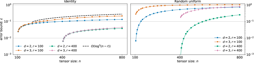
Figure 1: Low-rank tensor-train approximation errors in the maximum norm obtained with the method of quasioptimal alternating projections for the varying tensor size.

Appendix A Other proofs

A.1 Proof of Lemma 1.1

1. Let $\mathsf{A}=\mathsf{G}_{1}\mathbin{\Join}\cdots\mathbin{\Join}\mathsf{G}_{s}$ and $\mathsf{B}=\mathsf{G}_{s+1}\mathbin{\Join}\cdots\mathbin{\Join}\mathsf{G}_{d}$. By the definition of $\mathrm{Mat}_{s}(\bm{\mathsf{G}}^{\mathbin{\Join}})$,

$$\mathrm{Mat}_{s}(\bm{\mathsf{G}}^{\mathbin{\Join}})=\begin{bmatrix}\mathsf{A}^{\{{\mathsf{1,\ldots,1}}\}}\mathsf{B}^{\{{\mathsf{1,\ldots,1}}\}}&\mathsf{A}^{\{{\mathsf{1,\ldots,1}}\}}\mathsf{B}^{\{{\mathsf{1,\ldots,2}}\}}&\cdots&\mathsf{A}^{\{{\mathsf{1,\ldots,1}}\}}\mathsf{B}^{\{{\mathsf{n_{s+1},\ldots,n_{d}}}\}}\\ \mathsf{A}^{\{{\mathsf{2,\ldots,1}}\}}\mathsf{B}^{\{{\mathsf{1,\ldots,1}}\}}&\mathsf{A}^{\{{\mathsf{2,\ldots,1}}\}}\mathsf{B}^{\{{\mathsf{1,\ldots,2}}\}}&\cdots&\mathsf{A}^{\{{\mathsf{2,\ldots,1}}\}}\mathsf{B}^{\{{\mathsf{n_{s+1},\ldots,n_{d}}}\}}\\ \vdots&\vdots&&\vdots\\ \mathsf{A}^{\{{\mathsf{n_{1},\ldots,n_{s}}}\}}\mathsf{B}^{\{{\mathsf{1,\ldots,1}}\}}&\mathsf{A}^{\{{\mathsf{n_{1},\ldots,n_{s}}}\}}\mathsf{B}^{\{{\mathsf{1,\ldots,2}}\}}&\cdots&\mathsf{A}^{\{{\mathsf{n_{1},\ldots,n_{s}}}\}}\mathsf{B}^{\{{\mathsf{n_{s+1},\ldots,n_{d}}}\}}\\ \end{bmatrix}.$$

It then follows from the definition of $\mathrm{Mat}_{<}(\mathsf{A})$ and $\mathrm{Mat}_{>}(\mathsf{B})$ that

$$\mathrm{Mat}_{s}(\bm{\mathsf{G}}^{\mathbin{\Join}}) =\begin{bmatrix}\mathrm{Mat}_{<}(\mathsf{A})\mathsf{B}^{\{{\mathsf{1,\ldots,1}}\}}&\mathrm{Mat}_{<}(\mathsf{A})\mathsf{B}^{\{{\mathsf{1,\ldots,2}}\}}&\cdots&\mathrm{Mat}_{<}(\mathsf{A})\mathsf{B}^{\{{\mathsf{n_{s+1},\ldots,n_{d}}}\}}\end{bmatrix}$$

$$=\mathrm{Mat}_{<}(\mathsf{A})\cdot\mathrm{Mat}_{>}(\mathsf{B}).$$

2. Now, let $\mathsf{A}=\mathsf{G}_{1}\mathbin{\Join}\cdots\mathbin{\Join}\mathsf{G}_{s-1}$. Then we have

$$\mathrm{Mat}_{<}(\mathsf{A}\mathbin{\Join}\mathsf{G}_{s})=\begin{bmatrix}\mathsf{A}^{\{{\mathsf{1,\ldots,1}}\}}\mathsf{G}^{\{{\mathsf{1}}\}}_{s}\\ \vdots\\ \mathsf{A}^{\{{\mathsf{n_{1},\ldots,n_{s-1}}}\}}\mathsf{G}^{\{{\mathsf{1}}\}}_{s}\\ \mathsf{A}^{\{{\mathsf{1,\ldots,1}}\}}\mathsf{G}^{\{{\mathsf{2}}\}}_{s}\\ \vdots\\ \mathsf{A}^{\{{\mathsf{n_{1},\ldots,n_{s-1}}}\}}\mathsf{G}^{\{{\mathsf{n_{s}}}\}}_{s}\end{bmatrix}=\begin{bmatrix}\mathrm{Mat}_{<}(\mathsf{A})\mathsf{G}^{\{{\mathsf{1}}\}}_{s}\\ \mathrm{Mat}_{<}(\mathsf{A})\mathsf{G}^{\{{\mathsf{2}}\}}_{s}\\ \vdots\\ \mathrm{Mat}_{<}(\mathsf{A})\mathsf{G}^{\{{\mathsf{n_{s}}}\}}_{s}\\ \end{bmatrix}=[I_{n_{s}}\otimes\mathrm{Mat}_{<}(\mathsf{A})]\begin{bmatrix}\mathsf{G}^{\{{\mathsf{1}}\}}_{s}\\ \vdots\\ \mathsf{G}^{\{{\mathsf{n_{s}}}\}}_{s}\end{bmatrix}.$$

3. The proof for the right unfolding is similar. ∎

A.2 Proof of Lemma 3.1

Consider the QR decomposition of the left unfolding $\mathrm{Mat}_{<}(\mathsf{G})=\bm{Q}\bm{R}$ with $\bm{Q}\in\mathbb{R}^{pn_{\ast}\times\hat{q}}$ such that $\bm{Q}^{\top}\bm{Q}=I_{\hat{q}}$ and $\bm{R}\in\mathbb{R}^{\hat{q}\times q}$ and let $\bm{Q}^{\top}=\begin{bmatrix}\bm{Q}_{1}^{\top}&\cdots&\bm{Q}_{n_{\ast}}^{\top}\end{bmatrix}$. Then for every index $\bm{{\mathsf{i}}}=({\mathsf{i}}_{1},\ldots,{\mathsf{i}}_{l})$ and $i={\mathsf{i}}_{1}+\sum_{s=2}^{l}({\mathsf{i}}_{s}-1)(n_{1}\ldots n_{s-1})$, we have $\mathsf{G}^{\{{\mathsf{\bm{{\mathsf{i}}}}}\}}=\bm{Q}_{i}\bm{R}$. By [25, Corollary 3.5.10], we have

$$\|\mathsf{G}^{\{{\mathsf{\bm{{\mathsf{i}}}}}\}}\|_{\mathrm{u}}=\|\bm{Q}_{i}\bm{R}\|_{\mathrm{u}}\leq\|\bm{Q}_{i}\|_{\mathrm{u}}\cdot\|\bm{R}\|_{\mathrm{sp}}=\|\bm{Q}_{i}\|_{\mathrm{u}}\cdot\|\mathrm{Mat}_{<}(\mathsf{G})\|_{\mathrm{sp}}.$$

As the columns of $\bm{Q}$ span the range of $\mathrm{Mat}_{<}(\mathsf{G})$, it holds that $\mu_{<}(\mathsf{G},\|\cdot\|_{\mathrm{u}})=\frac{n_{\ast}p}{\hat{q}}\max_{i\in[N]}\|\bm{Q}_{i}\|_{\mathrm{u}}$. The second inequality can be proved similarly. ∎

A.3 Proof of Lemma 3.2

1. Consider the first unfoldings $\mathrm{Mat}_{1}(\bm{\mathsf{L}}^{\mathbin{\Join}})=\mathrm{Mat}_{1}(\bm{\mathsf{S}}^{\mathbin{\Join}})$. By Lemma 1.1,

$$\mathrm{Mat}_{<}(\mathsf{L}_{1})\mathrm{Mat}_{>}(\mathsf{L}_{2}\mathbin{\Join}\cdots\mathbin{\Join}\mathsf{L}_{d})=\mathrm{Mat}_{<}(\mathsf{S}_{1})\mathrm{Mat}_{>}(\mathsf{S}_{2}\mathbin{\Join}\cdots\mathbin{\Join}\mathsf{S}_{d}).$$

Since $\bm{\mathsf{L}}$ and $\bm{\mathsf{S}}$ are minimal, the columns of $\mathrm{Mat}_{<}(\mathsf{L}_{1})$ and $\mathrm{Mat}_{<}(\mathsf{S}_{1})$ span the same subspace, thus $\mu_{<}(\mathsf{S}_{1},\|\cdot\|_{\mathrm{u}})=\mu_{<}(\mathsf{L}_{1},\|\cdot\|_{\mathrm{u}})$. If $s=1$ or $d=2$, we are done. Otherwise, $\mathsf{S}_{1}$ is left-orthogonal and there exists an orthogonal matrix $\bm{Q}_{1}$ such that $\mathrm{Mat}_{<}(\mathsf{S}_{1})=\mathrm{Mat}_{<}(\mathsf{L}_{1})\bm{Q}_{1}$. We can define a new core $\mathsf{\hat{S}}_{2}$ by $\mathsf{\hat{S}}^{\{{\mathsf{i}}\}}_{2}=\bm{Q}_{1}\mathsf{S}^{\{{\mathsf{i}}\}}_{2}$, which satisfies $\mu_{<}(\mathsf{\hat{S}}_{2},\|\cdot\|_{\mathrm{u}})=\mu_{<}(\mathsf{S}_{2},\|\cdot\|_{\mathrm{u}})$ since the norm is unitarily invariant, and is left-orthogonal if $\mathsf{S}_{2}$ is. Then the TT representation $\bm{\mathsf{G}}_{2}=(\mathsf{L}_{1},\mathsf{\hat{S}}_{2},\mathsf{S}_{3},\ldots,\mathsf{S}_{d})$ is minimal, $s$-orthogonal and satisfies $\bm{\mathsf{G}}_{2}^{\mathbin{\Join}}=\bm{\mathsf{L}}^{\mathbin{\Join}}$.

We proceed by induction over $\hat{t}\leq\min\{s,d-1\}$. Assume that $\mu_{<}(\mathsf{S}_{t},\|\cdot\|_{\mathrm{u}})=\mu_{<}(\mathsf{L}_{t},\|\cdot\|_{\mathrm{u}})$ holds for all $t<\hat{t}$ and there exists a TT representation $\bm{\mathsf{G}}_{\hat{t}}=(\mathsf{L}_{1},\ldots,\mathsf{L}_{\hat{t}-1},\mathsf{\hat{S}}_{\hat{t}},\mathsf{S}_{\hat{t}+1},\ldots,\mathsf{S}_{d})$ that is minimal, $s$-orthogonal, satisfies $\bm{\mathsf{G}}_{\hat{t}}^{\mathbin{\Join}}=\bm{\mathsf{L}}^{\mathbin{\Join}}$ and $\mu_{<}(\mathsf{\hat{S}}_{\hat{t}},\|\cdot\|_{\mathrm{u}})=\mu_{<}(\mathsf{S}_{\hat{t}},\|\cdot\|_{\mathrm{u}})$. We can repeat the previous argument. Consider the unfoldings $\mathrm{Mat}_{\hat{t}}(\bm{\mathsf{L}}^{\mathbin{\Join}})=\mathrm{Mat}_{\hat{t}}(\bm{\mathsf{G}}_{{\hat{t}}}^{\mathbin{\Join}})$. By Lemma 1.1,

$$\mathrm{Mat}_{<}(\mathsf{L}_{1}\mathbin{\Join}\cdots\mathbin{\Join}\mathsf{L}_{\hat{t}})\mathrm{Mat}_{>}(\mathsf{L}_{\hat{t}+1}\mathbin{\Join}\cdots\mathbin{\Join}\mathsf{L}_{d})=\mathrm{Mat}_{<}(\mathsf{L}_{1}\mathbin{\Join}\cdots\mathbin{\Join}\mathsf{\hat{S}}_{\hat{t}})\mathrm{Mat}_{>}(\mathsf{S}_{\hat{t}+1}\mathbin{\Join}\cdots\mathbin{\Join}\mathsf{S}_{d}),$$

$$\mathrm{Mat}_{<}(\mathsf{L}_{1}\mathbin{\Join}\cdots\mathbin{\Join}\mathsf{L}_{\hat{t}})=[\bm{I}_{n_{\hat{t}}}\otimes\mathrm{Mat}_{<}(\mathsf{L}_{1}\mathbin{\Join}\cdots\mathbin{\Join}\mathsf{L}_{\hat{t}-1})]\cdot\mathrm{Mat}_{<}(\mathsf{L}_{\hat{t}}),$$

$$\mathrm{Mat}_{<}(\mathsf{L}_{1}\mathbin{\Join}\cdots\mathbin{\Join}\mathsf{\hat{S}}_{\hat{t}})=[\bm{I}_{n_{\hat{t}}}\otimes\mathrm{Mat}_{<}(\mathsf{L}_{1}\mathbin{\Join}\cdots\mathbin{\Join}\mathsf{L}_{\hat{t}-1})]\cdot\mathrm{Mat}_{<}(\mathsf{\hat{S}}_{\hat{t}}).$$

Since $\bm{\mathsf{L}}$ and $\bm{\mathsf{\bm{\mathsf{G}}}}_{{\hat{t}}}$ are minimal and $\bm{I}_{n_{\hat{t}}}\otimes\mathrm{Mat}_{<}(\mathsf{L}_{1}\mathbin{\Join}\cdots\mathbin{\Join}\mathsf{L}_{\hat{t}-1})$ is full rank, the columns of $\mathrm{Mat}_{<}(\mathsf{L}_{\hat{t}})$ and $\mathrm{Mat}_{<}(\mathsf{\hat{S}}_{\hat{t}})$ span the same subspace, hence $\mu_{<}(\mathsf{L}_{\hat{t}},\|\cdot\|_{\mathrm{u}})=\mu_{<}(\mathsf{\hat{S}}_{\hat{t}},\|\cdot\|_{\mathrm{u}})=\mu_{<}(\mathsf{S}_{\hat{t}},\|\cdot\|_{\mathrm{u}})$. The proof is finished if $\hat{t}=\min\{s,d-1\}$. Otherwise, $\mathsf{\hat{S}}_{\hat{t}}$ is left-orthogonal and there exists an orthogonal matrix $\bm{Q}_{{\hat{t}}}$ such that $\mathrm{Mat}_{<}(\mathsf{\hat{S}}_{\hat{t}})=\mathrm{Mat}_{<}(\mathsf{L}_{\hat{t}})\bm{Q}_{\hat{t}}$. We define a core $\mathsf{\hat{S}}_{{\hat{t}}+1}$ by $\mathsf{\hat{S}}^{\{{\mathsf{i}}\}}_{{\hat{t}}+1}=\bm{Q}_{\hat{t}}\mathsf{S}^{\{{\mathsf{i}}\}}_{{\hat{t}}+1}$ and a TT representation $\bm{\mathsf{G}}_{\hat{t}+1}=(\mathsf{L}_{1},\ldots,\mathsf{L}_{\hat{t}},\mathsf{\hat{S}}_{\hat{t}+1},\mathsf{S}_{\hat{t}+2},\ldots,\mathsf{S}_{d})$. This TT representation satisfies all the required assumptions, and we repeat the argument until $\min\{s,d-1\}$.

2. The proof for the right coherences can be carried out in the same way by moving right-to-left along the TT representations $\bm{\mathsf{R}}$ and $\bm{\mathsf{S}}$. ∎

A.4 Proof of Lemma 3.3

We prove the first part of the lemma, the second part being similar. For $s<d$, Lemma 1.1 gives

$$\mathrm{Mat}_{s}(\bm{\mathsf{S}}^{\mathbin{\Join}}) =\mathrm{Mat}_{<}(\mathsf{S}_{1}\mathbin{\Join}\cdots\mathbin{\Join}\mathsf{S}_{s})\cdot\mathrm{Mat}_{>}(\mathsf{S}_{s+1}\mathbin{\Join}\cdots\mathbin{\Join}\mathsf{S}_{d})$$

$$=[\bm{I}_{n_{s}}\otimes\mathrm{Mat}_{<}(\mathsf{S}_{1}\mathbin{\Join}\cdots\mathbin{\Join}\mathsf{S}_{s-1})]\cdot\mathrm{Mat}_{<}(\mathsf{S}_{s})\cdot\mathrm{Mat}_{>}(\mathsf{S}_{s+1}\mathbin{\Join}\cdots\mathbin{\Join}\mathsf{S}_{d}).$$

By Lemma 1.1 and $s$-orthogonality, the left and right factors have orthonormal columns and rows, respectively. Then the singular values of $\mathrm{Mat}_{s}(\bm{\mathsf{S}}^{\mathbin{\Join}})$ and $\mathrm{Mat}_{<}(\mathsf{S}_{s})$ coincide. ∎

A.5 Proof of Lemma 4.6

We will prove the lemma by induction over the cardinality $|\Omega|$. For the base case, let $\Omega=\{\omega\}$ be a singleton. There are two partitions of $\Omega^{2}$:

$$\pi_{1}=\bigg{\{}\big{\{}(\omega,1),(\omega,2)\big{\}}\bigg{\}},\quad\pi_{2}=\bigg{\{}\big{\{}(\omega,1)\big{\}},\big{\{}(\omega,2)\big{\}}\bigg{\}}.$$

Fix $\pi_{1}$. Then $\kappa=1$ and $\Omega_{1}=\Omega=\{\omega\}$. It follows from Cauchy–Schwarz that

$$\sum_{\bm{{\mathsf{\alpha}}}\in[R]}\prod_{s\in[\kappa]}\mathcal{C}_{\bm{{\mathsf{\alpha_{\Omega_{s}}}}}}^{(s)}=\sum_{{\mathsf{\alpha}}_{\omega}\in[R(\omega)]}\mathcal{C}_{\bm{{\mathsf{\alpha_{\omega}}}}}^{(1)}\leq\sqrt{R(\omega)}\cdot\|\bm{\mathcal{C}}{}^{(1)}\|_{\mathrm{F}}=R(\omega)^{\theta_{\pi_{1}}(\omega)}\cdot\|\bm{\mathcal{C}}{}^{(1)}\|_{\mathrm{F}}.$$

Now, fix $\pi_{2}$. Then $\kappa=2$ and $\Omega_{1}=\Omega_{2}=\Omega=\{\omega\}$. Similarly, we obtain

$$\sum_{\bm{{\mathsf{\alpha}}}\in[R]}\prod_{s\in[\kappa]}\mathcal{C}_{\bm{{\mathsf{\alpha_{\Omega_{s}}}}}}^{(s)}=\sum_{{\mathsf{\alpha}}_{\omega}\in[R(\omega)]}\mathcal{C}_{\bm{{\mathsf{\alpha_{\omega}}}}}^{(1)}\mathcal{C}_{\bm{{\mathsf{\alpha_{\omega}}}}}^{(2)}\leq\|\bm{\mathcal{C}}{}^{(1)}\|_{\mathrm{F}}\|\bm{\mathcal{C}}{}^{(2)}\|_{\mathrm{F}}=R(\omega)^{\theta_{\pi_{2}}(\omega)}\cdot\|\bm{\mathcal{C}}{}^{(1)}\|_{\mathrm{F}}\|\bm{\mathcal{C}}{}^{(2)}\|_{\mathrm{F}}.$$

Next, consider axes $\Omega$ with $|\Omega|\geq 2$ and assume that the lemma holds for all axes of cardinality at most $|\Omega|-1$. Fix some $\pi=\{\mho_{1},\ldots,\mho_{\kappa}\}\in\mathscr{P}_{\kappa}(\Omega^{2})$ and pick $\omega\in\Omega$. Suppose $\theta_{\pi}(\omega)=1/2$, that is $\omega$ belongs to exactly one $\Omega_{t}=\mathrm{condense}(\mho_{t})\subseteq\Omega$. Then by Cauchy–Schwarz we get

$$\sum_{\bm{{\mathsf{\alpha}}}\in[R]}\prod_{s\in[\kappa]}\mathcal{C}_{\bm{{\mathsf{\alpha_{\Omega_{s}}}}}}^{(s)} =\sum_{\bm{{\mathsf{\alpha^{\prime}}}}\in[R_{\Omega\setminus\{\omega\}}]}\left(\sum_{\alpha_{\omega}\in[R(\omega)]}\mathcal{C}_{\bm{{\mathsf{\alpha_{\omega}\dot{\times}\alpha^{\prime}_{\Omega_{t}\setminus\{\omega\}}}}}}^{(t)}\right)\prod_{s\neq t}\mathcal{C}_{\bm{{\mathsf{\alpha^{\prime}_{\Omega_{s}}}}}}^{(s)}$$

$$\leq\sqrt{R(\omega)}\sum_{\bm{{\mathsf{\alpha^{\prime}}}}\in[R_{\Omega\setminus\{\omega\}}]}\mathrm{Frob}_{\{\omega\}}(\bm{\mathcal{C}}{}^{(t)})_{\bm{{\mathsf{\alpha^{\prime}_{\Omega_{t}\setminus\{\omega\}}}}}}\prod_{s\neq t}\mathcal{C}_{\bm{{\mathsf{\alpha^{\prime}_{\Omega_{s}}}}}}^{(s)}.$$

This removes the presence of $\omega$ from the sum and reduces the problem to the case of smaller axes $\Omega^{\prime}=\Omega\setminus\{\omega\}$. We can modify $\pi$ to construct a partition $\pi^{\prime}$ of $\Omega^{\prime 2}$. By our assumption $\theta_{\pi}(\omega)=1/2$, there are two possibilities:

$$\pi^{\prime}=\begin{cases}\pi\setminus\mho_{t}\in\mathscr{P}_{\kappa-1}(\Omega^{\prime 2}),&\mho_{t}\setminus\big{\{}(\omega,1),(\omega,2)\big{\}}=\varnothing,\\ \{\mho_{1},\ldots,\mho_{t}\setminus\big{\{}(\omega,1),(\omega,2)\big{\}},\ldots,\mho_{\kappa}\}\in\mathscr{P}_{\kappa}(\Omega^{\prime 2}),&\mho_{t}\setminus\big{\{}(\omega,1),(\omega,2)\big{\}}\neq\varnothing.\end{cases}$$

Note that $\theta_{\pi}$ and $\theta_{\pi^{\prime}}$ coincide on $\Omega^{\prime}$. Then the induction hypothesis and Lemma 4.1 give

$$\sum_{\bm{{\mathsf{\alpha}}}\in[R]}\prod_{s\in[\kappa]}\mathcal{C}_{\bm{{\mathsf{\alpha_{\Omega_{s}}}}}}^{(s)}\leq\prod_{\omega\in\Omega}R(\omega)^{\theta_{\pi}(\omega)}\cdot\|\mathrm{Frob}_{\{\omega\}}(\bm{\mathcal{C}}{}^{(t)})\|_{\mathrm{F}}\prod_{s\neq t}\|\bm{\mathcal{C}}{}^{(s)}\|_{\mathrm{F}}=\prod_{\omega\in\Omega}R(\omega)^{\theta_{\pi}(\omega)}\prod_{s\in[\kappa]}\|\bm{\mathcal{C}}{}^{(s)}\|_{\mathrm{F}}.$$

Suppose now that $\theta_{\pi}(\omega)=0$, i.e. $\omega$ belongs to two distinct subaxes $\Omega_{t},\Omega_{p}\subseteq\Omega$. Then a similar argument leads us to

$$\sum_{\bm{{\mathsf{\alpha}}}\in[R]}\prod_{s\in[\kappa]}\mathcal{C}_{\bm{{\mathsf{\alpha_{\Omega_{s}}}}}}^{(s)} =\sum_{\bm{{\mathsf{\alpha^{\prime}}}}\in[R_{\Omega\setminus\{\omega\}}]}\left(\sum_{\alpha_{\omega}\in[R(\omega)]}\mathcal{C}_{\bm{{\mathsf{\alpha_{\omega}\dot{\times}\alpha^{\prime}_{\Omega_{t}\setminus\{\omega\}}}}}}^{(t)}\mathcal{C}_{\bm{{\mathsf{\alpha_{\omega}\dot{\times}\alpha^{\prime}_{\Omega_{p}\setminus\{\omega\}}}}}}^{(p)}\right)\prod_{s\neq t,p}\mathcal{C}_{\bm{{\mathsf{\alpha^{\prime}_{\Omega_{s}}}}}}^{(s)}$$

$$\leq\sum_{\bm{{\mathsf{\alpha^{\prime}}}}\in[R_{\Omega\setminus\{\omega\}}]}\mathrm{Frob}_{\{\omega\}}(\bm{\mathcal{C}}{}^{(t)})_{\bm{{\mathsf{\alpha^{\prime}_{\Omega_{t}\setminus\{\omega\}}}}}}\mathrm{Frob}_{\{\omega\}}(\bm{\mathcal{C}}{}^{(p)})_{\bm{{\mathsf{\alpha^{\prime}_{\Omega_{p}\setminus\{\omega\}}}}}}\prod_{s\neq t,p}\mathcal{C}_{\bm{{\mathsf{\alpha^{\prime}_{\Omega_{s}}}}}}^{(s)}.$$

We can build a partition $\pi^{\prime}$ of $\Omega^{\prime 2}$ such that $\theta_{\pi}=\theta_{\pi^{\prime}}$ on $\Omega^{\prime}$ and the number of cells is equal to

$$|\pi^{\prime}|=\begin{cases}\kappa-2,&\text{both}\leavevmode\nobreak\ \mho_{t},\mho_{p}\leavevmode\nobreak\ \text{are singletons},\\ \kappa-1,&\text{one of}\leavevmode\nobreak\ \mho_{t},\mho_{p}\leavevmode\nobreak\ \text{is a singleton},\\ \kappa,&\text{neither of}\leavevmode\nobreak\ \mho_{t},\mho_{p}\leavevmode\nobreak\ \text{is a singleton}.\end{cases}$$

It remains to use the induction hypothesis and Lemma 4.1. ∎

References

- [1] Guifré Vidal “Efficient classical simulation of slightly entangled quantum computations” In Phys Rev Lett 91.14 APS, 2003, pp. 147902 DOI: 10.1103/PhysRevLett.91.147902
- [2] I. Oseledets and E. Tyrtyshnikov “TT-cross approximation for multidimensional arrays” In Linear Algebra Appl 432.1 Elsevier, 2010, pp. 70–88 DOI: 10.1016/j.laa.2009.07.024
- [3] Ulrich Schollwöck “The density-matrix renormalization group in the age of matrix product states” In Ann Phys 326.1 Elsevier, 2011, pp. 96–192 DOI: 10.1016/j.aop.2010.09.012
- [4] I.V. Oseledets “Tensor-train decomposition” In SIAM J Sci Comput 33.5 SIAM, 2011, pp. 2295–2317 DOI: 10.1137/090752286
- [5] Vladimir A Kazeev and Boris N Khoromskij “Low-rank explicit QTT representation of the Laplace operator and its inverse” In SIAM J Matrix Anal Appl 33.3 SIAM, 2012, pp. 742–758 DOI: 10.1137/110844830
- [6] Vladimir A Kazeev, Boris N Khoromskij and Eugene E Tyrtyshnikov “Multilevel Toeplitz matrices generated by tensor-structured vectors and convolution with logarithmic complexity” In SIAM J Sci Comput 35.3 SIAM, 2013, pp. A1511–A1536 DOI: 10.1137/110844830
- [7] Markus Bachmayr and Vladimir Kazeev “Stability of low-rank tensor representations and structured multilevel preconditioning for elliptic PDEs” In Found Comput Math 20.5 Springer, 2020, pp. 1175–1236 DOI: 10.1007/s10208-020-09446-z
- [8] Warwick De Launey and Jennifer Seberry “The strong Kronecker product” In J Comb Theory A 66.2 Elsevier, 1994, pp. 192–213 DOI: 10.1016/0097-3165(94)90062-0
- [9] S.A. Goreinov, E.E. Tyrtyshnikov and N.L. Zamarashkin “A theory of pseudoskeleton approximations” In Linear Algebra Appl 261.1-3 Elsevier, 1997, pp. 1–21 DOI: 10.1016/S0024-3795(96)00301-1
- [10] SA Goreinov and EE Tyrtyshnikov “The maximal-volume concept in approximation by low-rank matrices” In Contemp Math 280, 2001, pp. 47–51 DOI: 10.1090/conm/280
- [11] D.V. Savostyanov “Quasioptimality of maximum-volume cross interpolation of tensors” In Linear Algebra Appl 458 Elsevier, 2014, pp. 217–244 DOI: 10.1016/j.laa.2014.06.006
- [12] N. Alon et al. “The approximate rank of a matrix and its algorithmic applications: approximate rank” In Proceedings of the 45th Annual ACM Symposium on Theory of Computing, 2013, pp. 675–684 DOI: 10.1145/2488608.2488694
- [13] M. Udell and A. Townsend “Why are big data matrices approximately low rank?” In SIAM J Math Data Sci 1.1 SIAM, 2019, pp. 144–160 DOI: 10.1137/18M1183480
- [14] S. Budzinskiy “On the distance to low-rank matrices in the maximum norm” In Linear Algebra Appl 688, 2024, pp. 44–58 DOI: 10.1016/j.laa.2024.02.012
- [15] Stanislav Budzinskiy and Nikolai Zamarashkin “Tensor train completion: local recovery guarantees via Riemannian optimization” In Numer Linear Algebra Appl 30.6 Wiley Online Library, 2023, pp. e2520 DOI: 10.1002/nla.2520
- [16] A. Sultonov, S. Matveev and S. Budzinskiy “Low-rank nonnegative tensor approximation via alternating projections and sketching” In Comput Appl Math 42.2 Springer, 2023, pp. 68 DOI: 10.1007/s40314-023-02211-2
- [17] S. Budzinskiy “Quasioptimal alternating projections and their use in low-rank approximation of matrices and tensors”, 2023 arXiv:2308.16097
- [18] Frank L Hitchcock “The expression of a tensor or a polyadic as a sum of products” In J Math Phys 6.1-4 Wiley Online Library, 1927, pp. 164–189 DOI: 10.1002/sapm192761164
- [19] Tamara G Kolda and Brett W Bader “Tensor decompositions and applications” In SIAM Rev 51.3 SIAM, 2009, pp. 455–500 DOI: 10.1137/07070111x
- [20] Stefan Bamberger, Felix Krahmer and Rachel Ward “The Hanson–Wright inequality for random tensors” In Sampl Theory Signal Process Data Anal 20.2 Springer, 2022, pp. 14 DOI: 10.1007/s43670-022-00028-4
- [21] Miaoyan Wang et al. “Operator norm inequalities between tensor unfoldings on the partition lattice” In Linear Algebra Appl 520 Elsevier, 2017, pp. 44–66 DOI: 10.1016/j.laa.2017.01.017
- [22] Rafał Latała “Estimates of moments and tails of Gaussian chaoses” In Ann Probab 34.6 Institute of Mathematical Statistics, 2006, pp. 2315–2331 DOI: 10.1214/009117906000000421
- [23] N. Gillis and Y. Shitov “Low-rank matrix approximation in the infinity norm” In Linear Algebra Appl 581 Elsevier, 2019, pp. 367–382 DOI: 10.1016/j.laa.2019.07.017
- [24] Stanislav Morozov, Matvey Smirnov and Nikolai Zamarashkin “On the optimal rank-1 approximation of matrices in the Chebyshev norm” In Linear Algebra Appl 679 Elsevier, 2023, pp. 4–29 DOI: 10.1016/j.laa.2023.09.007
- [25] Roger A. Horn and Charles R. Johnson “Topics in matrix analysis” isbn: 9780521467131 CUP, 1994