We obtained new hairy black hole solutions in Einstein-scalar theory, including asymptotic flat, de Sitter and anti-de Sitter black holes. The theory is inspired by Ref. [1], where traversable wormhole solutions from an Einstein-phantom scalar theory are constructed. In this work, we found new black hole solutions in an Einstein-normal scalar theory. Comparing with Schwarzschild metric, the hairy black holes have two interesting properties: i) the areas of the black holes are always smaller than the same mass Schwarzschild black holes; ii) A naked singularity with positive mass arises when the black hole mass decreases. The energy conditions for the black holes and naked singularities are checked. We found that, as hairy black holes, the null energy condition(NEC) and the strong energy condition(SEC) are hold, while the weak energy condition(WEC) is violated in the vicinity of black hole horizon. The naked singularity respects to all three energy conditions. We also investigate the quasinormal modes(QNMs) of the hairy black holes by a test scalar field. The results indicate that one can distinguish hairy black holes with the same mass Schwarzschilid black hole by their QNM spectra.

xiaopingrao@jxnu.edu.cn
hyat@mail.bnu.edu.cn
yangjinbo@gzhu.edu.cn

1 Introduction

The study of black holes is quite prominent nowadays because of the shadow images cast by the M87* black hole[2] and the Sagittarius A* black hole [3]. On the other hand, the detection of gravitational waves (GWs) originated from the merger of binary black holes in 2015 laid the conceptual cornerstone for gravitational detections [4]. These great progresses in experiments provide fruitful data to the theoretical studies of black holes and hence have launched an extraordinary new era in black hole physics. Therefore, more and more gravitational experiments are being planned or are already underway, such as the LISA in Europe/USA, KAGRA in Japan, GEO600 in Germany, Taiji and Tianqin in China [8, 7, 6, 9, 5, 11, 12, 10, 13].

In theory, the no-hair conjecture plays a pivotal role in black hole physics. The uniqueness of Schwarzschild black hole and Kerr black hole has been demonstrated (see Ref. [14, 15, 16, 17, 18]), which state that one can describe a stationary black hole solely in terms of its mass $M$, and angular momentum $J$. The idea of testing the no-hair conjecture with black hole shadow images and GWs has caused widespread concern [19, 20, 21, 22, 23, 24, 25, 26, 27, 28]. However, we can’t rule out the existence of hairy black holes yet. In fact, many black holes with scalar hair [29, 30, 31, 32, 33, 34, 35, 36, 37, 38, 39], Yang-Mills hair[40, 41, 42, 43, 44, 45], and so on[46, 47, 48, 49] have been constructed. These hairy black holes are so attractive that there are numerous theoretical studies on their properties [50, 51, 52, 53] and experimental constraints [54, 19, 55, 56].

Black hole with scalar hair, namely imposing a scalar field into the Einstein gravity, is the simplest example of hairy black holes. Although the only scalar degree of freedom in the Standard Model (SM) is the Higgs field, scalar fields are utilized in numerous aspects of fundamental physics, like the dark matter (DM) candidates including axion-like particles (ALP)[57, 58, 59, 62, 60, 61], the nature of dynamical dark energy[63, 64], and inflatons in many usually considered inflation models[65, 66]. As in string theory, scalar fields appear in several contexts: the so-called dilaton generally appears as a kind of variation mode on a string; the moduli massless scalars or axions from higher-form fields emerge when compactifying six extra dimensions[67, 68, 69]. Despite Bekenstein’s investigation from 1971 on the General Relativity minimally coupled to a scalar field, which resulted in a no-scalar hair theorem (originating in [70, 71, 72, 73] and reviewed in [74]). It is possible to circumvent some of the assumptions he made to obtain hairy black holes. Such as by introducing higher-order derivative gravities like the Gauss-Bonnet term, non-minimally coupled to the scalar field. This may give rise to an intriguing phenomenon known as “black hole scalarization”, wherein non-hairy black holes can evolve and spontaneously develop scalar hair themselves[76, 77, 75, 78, 79, 80].

Another path to bypass the no-scalar hair theorem is by violating the energy conditions, especially the weak energy condition. In around 1970s, R. Penrose and S. Hawking came up with a series of works on singularity theorems, which require adherence to the energy conditions [81, 82, 83]. However, in both theoretical and experimental research, there remains a strong desire towards matters that violate energy conditions. A well-known example in quantum field theory is the Casimir effect, where the null energy condition could be violated[84, 85]. Based on cosmological observations, our Universe is undergoing accelerated expansion[86, 87, 88]. The cosmological constant can be treated as a dark energy model that supports this accelerated expansion and violates weak energy condition. Furthermore, the existence of exotic objects such as traversable wormholes also necessitates the violation of energy conditions[89, 90, 91, 92].

In this work, we examine the Einstein-scalar theory and construct hairy black hole solutions. The theory contains a scalar field with a potential inspired by Ref. [1]. We obtain hairy black holes whose asymptotic behavior can be (A)dS or Minkowski spacetime depending on the parameters. (A)dS black holes are attractive in holographic theories, but in astrophysics, asymptotically flat black holes are more realistic. We mainly discuss the asymptotic black hole solutions in this work. We find that the areas of hairy black holes are always smaller than those of Schwarzschild black holes with the same mass. As the scalar parameter $q$ approaches a critical value, the black hole area can become infinitesimally small, which may have significant observational implications. Hence, we examine their QNM’s spectra compared to those of Schwarzschild black holes with the same mass by evolving test scalar fields. The results show that the hairy black holes possess higher oscillation frequencies and shorter decay time. On the other hand, the black hole solutions can become naked singularities as the scalar parameter $q$ varies. We find that such naked singularities can satisfy null, strong, and weak energy conditions. However, the black hole solutions always violate the weak energy condition and thus do not violate the no-scalar hair theorem in Ref. [73]. Our study provides an analytical model for hairy black hole studies.

Our works are organized as follows. In section 2, we present the theory and the analytical black hole solution. Then we discuss the properties of the black holes in section 3 and examine the energy conditions in section 4. The QNMs of the test field are investigated in section 5. Finally, we conclude our work in section 6 and the appendix in the transformation to obtain the theory.

2 The theory and the solution

The Lagrangian for Einstein-scalar theories which is to be considered in our work is given by

$${\cal L}=\sqrt{-g}(R-{\textstyle{\frac{\scriptstyle 1}{\scriptstyle 2}}}(\partial\phi)^{2}-V(\phi)),$$ (1)

where $R$ is the scalar curvature, and $(\partial\phi)^{2}$ is $g^{\mu\nu}\partial_{\mu}\phi\,\partial_{\nu}\phi$ for short. While the scalar potential is

$$V(\phi)=\alpha\,U(\phi)+\beta\,U(-\phi)$$ (2)

with

$$U(\phi)=e^{-\sqrt{\gamma^{2}-1}\,\phi}\bigg{(}(2-3\gamma^{2})\,\text{cosh}(\gamma\phi)-3\gamma\sqrt{\gamma^{2}-1}\,\text{sinh}(\gamma\phi)-2\bigg{)}.$$ (3)

The coefficients $\gamma$, $\beta$ and $\alpha$ in the scalar potential are three theoretical parameters with $\gamma>1$. Note that the potential (3) has the similar form to the Eq.(63) of Ref. [93] in $\phi\to i\phi$.

The equations of motion (E.O.Ms) associated with the variation of $\phi$ and $g^{\mu\nu}$ are respectively given by

$$\Box\phi={\frac{\partial V}{\partial\phi}}\,,$$ (4)

$$E_{\mu\nu}\equiv R_{\mu\nu}-{\textstyle{\frac{\scriptstyle 1}{\scriptstyle 2}}}Rg_{\mu\nu}-T_{\mu\nu}^{\phi}=0\,,$$ (5)

where

$$T_{\mu\nu}^{\phi}=\bigg{(}{\textstyle{\frac{\scriptstyle 1}{\scriptstyle 2}}}\partial_{\mu}\phi\partial_{\nu}\phi-{\textstyle{\frac{\scriptstyle 1}{\scriptstyle 4}}}g_{\mu\nu}(\partial\phi)^{2}\bigg{)}-{\textstyle{\frac{\scriptstyle 1}{\scriptstyle 2}}}g_{\mu\nu}V.$$ (6)

We consider the spherically symmetric and static ansatz

$$ds^{2}=-hdt^{2}+f^{-1}dr^{2}+R^{2}d\Omega_{2}^{2},\qquad\phi=\phi(r),$$ (7)

where $d\Omega^{2}_{2}=d\theta^{2}+\sin^{2}\theta d\varphi^{2}$ the $2$-sphere and $(h,f,R)$ are the metric functions of $r$. Substitutes this ansatz into (4) gives four equations, which are given by

$$-4+4fR^{\prime 2}+R^{2}(2V+f\phi^{\prime 2})+4R(2fR^{\prime\prime}+f^{\prime}R^{\prime})=0,$$

$$-4h+4hfR^{\prime 2}+2hR^{2}V-hfR^{2}\phi^{\prime 2}+4fRR^{\prime}h^{\prime}=0,$$

$$R(2hfh^{\prime\prime}+h^{2}(f\phi^{\prime 2}+2V))+R(hh^{\prime}f^{\prime}-fh^{\prime 2})+2R^{\prime}(fhh^{\prime}+h^{2}f^{\prime})+4h^{\prime}fR^{\prime\prime}=0,$$

$$R\phi^{\prime}(hf)^{\prime}+2hf(2R^{\prime}\phi^{\prime}+R\phi^{\prime\prime})-2hR{\frac{\partial V}{\partial\phi}}=0,$$ (8)

where a prime denotes the derivative with respect to $r$. It is easy to find that the scalar equations of motion are automatically satisfied provided that the above equations are satisfied, and hence only three independent equations left here. It’s straightforward to check the following solution satisfies all the E.O.Ms (2)

$$ds^{2} = -h(r)dt^{2}+f(r)^{-1}dr^{2}+R(r)^{2}d\Omega_{2}^{2},\qquad R(r)^{2}=e^{-\sqrt{\gamma^{2}-1}\phi}r^{2},\qquad f=h{\frac{r^{2}+q^{2}\gamma^{2}}{r^{2}}},$$

$$h = {\frac{\alpha}{2}}e^{-\sqrt{\gamma^{2}-1}\phi}\gamma^{2}r^{2}+{\frac{\beta}{2}}e^{\sqrt{\gamma^{2}-1}\phi}\gamma^{2}\big{(}r^{2}+q^{2}\gamma^{2}-4q\sqrt{r^{2}+q^{2}\gamma^{2}}\sqrt{\gamma^{2}-1}+q^{2}(7\gamma^{2}-8)\big{)}$$

$$+e^{\sqrt{\gamma^{2}-1}\phi},$$

$$\phi = {\frac{2}{\gamma}}\text{arctanh}({\frac{q\gamma}{\sqrt{r^{2}+q^{2}\gamma^{2}}}}),$$ (9)

and hence a solution of the Einstein-normal scalar theory. Analysis of the metric function yields the solution represents single-horizon black holes or time-like naked singularities. We expand the metric functions at $r\to\infty$,

$$h = -{\frac{\Lambda}{3}}r^{2}+{\frac{2}{3}}\Lambda\sqrt{\gamma^{2}-1}\,qr+\big{(}1-{\frac{2}{3}}\Lambda(\gamma^{2}-1)\,q^{2}\big{)}$$

$$\quad+{\frac{q\sqrt{\gamma^{2}-1}\bigg{(}18-q^{2}(3\gamma^{2}-4)(12\alpha\gamma^{2}+7\Lambda)\bigg{)}}{9r}}+...\,,$$

$$f = -{\frac{\Lambda}{3}}r^{2}+{\frac{2}{3}}\Lambda\sqrt{\gamma^{2}-1}\,qr+\big{(}1-\Lambda(\gamma^{2}-{\frac{2}{3}})\,q^{2}\big{)}+...\,,$$

$$R^{2} = r^{2}-2qr\sqrt{\gamma^{2}-1}+2q^{2}(\gamma^{2}-1)+...\,,$$ (10)

where $\Lambda$ is the effective cosmological constant, defined as

$$\Lambda\equiv-{\frac{3}{2}}(\alpha+\beta)\gamma^{2}\,.$$

It shows that the solution is asymptotic (A)dS or Minkowski spacetime depending on the value of $\Lambda$. AdS black holes can be served as concrete models of AdS/CFT and dS black holes are useful in the context of cosmology. However, as we mentioned in the introduction, our interest of this work is mainly in asymptotic flat black hole solutions.

3 Asymptotic flat black holes

The asymptotic flat solution arises in $\alpha+\beta$=0. Without loss of the generity, we set $\beta=-\alpha$, throughout the rest paper. According to (2), the mass of the solution can be read as

$$M={\frac{q\sqrt{\gamma^{2}-1}\bigg{(}2q^{2}\alpha\gamma^{2}(3\gamma^{2}-4)-3\bigg{)}}{3}}.$$ (11)

The positiveness of the mass requires

• $\alpha q^{2}>{\frac{3}{2\gamma^{2}(3\gamma^{2}-4)}}$, if $\gamma>{\frac{2}{\sqrt{3}}}$;

• $\alpha q^{2}<{\frac{3}{2\gamma^{2}(3\gamma^{2}-4)}}$, if $1<\gamma<{\frac{2}{\sqrt{3}}}$.

At $r\to 0$, we have

$$h(0)\sim\infty\bigg{(}1-2\alpha q^{2}\gamma^{2}(2\gamma^{2}-2-\gamma\sqrt{\gamma^{2}-1})\bigg{)}+\dots.$$ (12)

With respect to the positive mass condition, and make sure $h(0)$ is negative leads to black hole solutions, namely

• $\alpha q^{2}>{\textstyle{\frac{\scriptstyle-1}{\scriptstyle 2(2-2\gamma^{2}+\gamma\sqrt{\gamma^{2}-1})}}}$, if $\gamma>{\textstyle{\frac{\scriptstyle 2}{\scriptstyle\sqrt{3}}}}$;

• $\alpha q^{2}<{\textstyle{\frac{\scriptstyle-1}{\scriptstyle 2(2-2\gamma^{2}+\gamma\sqrt{\gamma^{2}-1})}}}$, if $1<\gamma<{\textstyle{\frac{\scriptstyle 2}{\scriptstyle\sqrt{3}}}}$.

Otherwise, it is a time-like naked singularity. For example, it represents a black hole with a horizon at $r_{h}=2.315$ and unit mass by setting $\gamma=2,q=0.2,\alpha=4.555$. We show the metric function in Fig.1. Another example is a time-like naked singularity, where $\gamma=2,q=0.1,\alpha=4.555$, as also shown in Fig. 1.

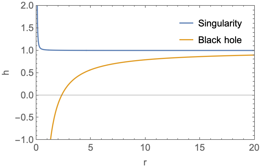
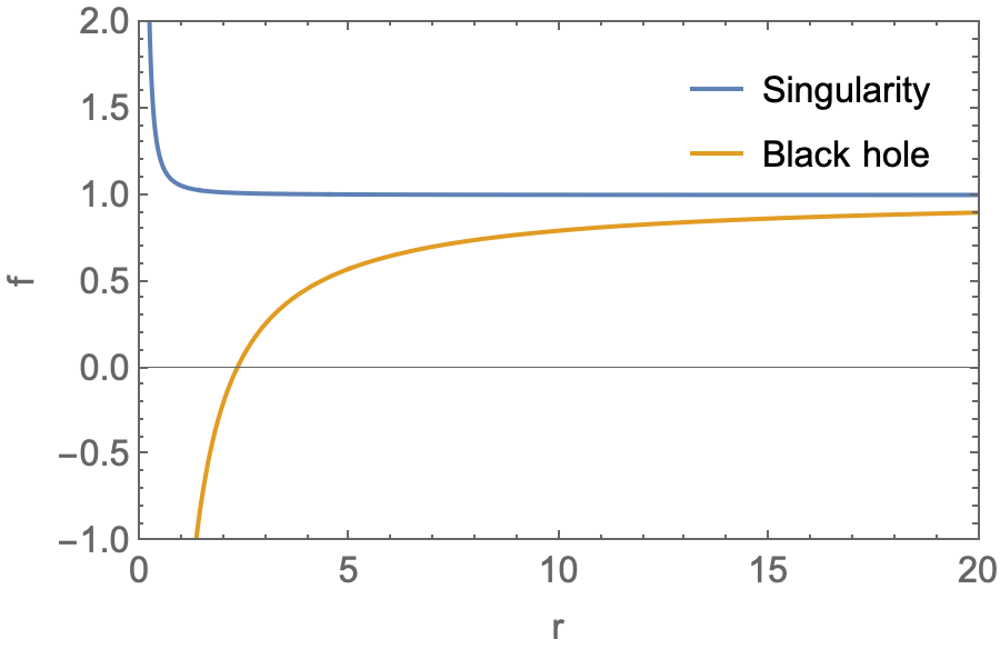
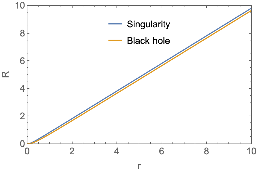
Figure 1: Examples of the metric functions $(h,f,R)$.

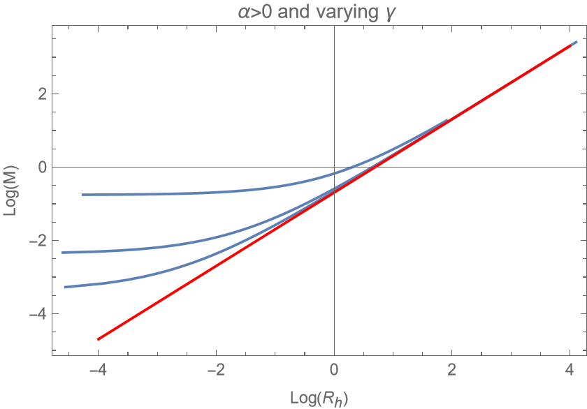
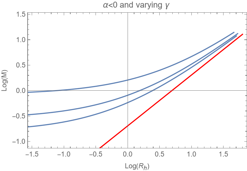
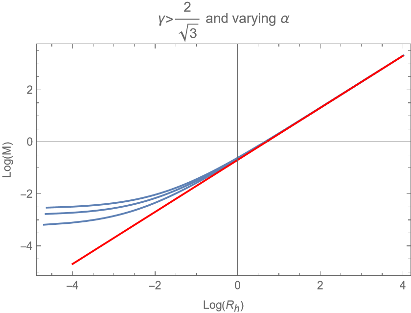
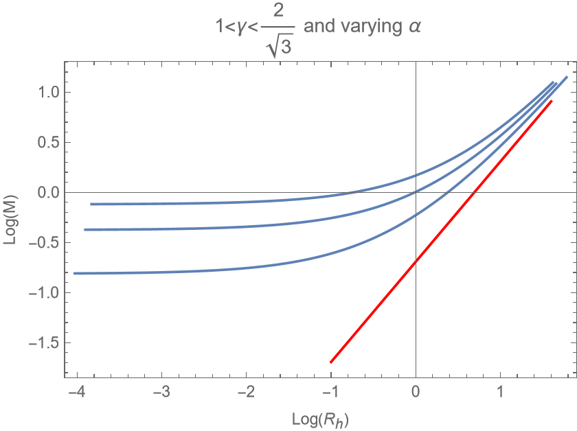
Figure 2: The relations between black hole mass and radius. The red lines denote standard Schwarzschild black holes and the blue lines denote hairy black holes.

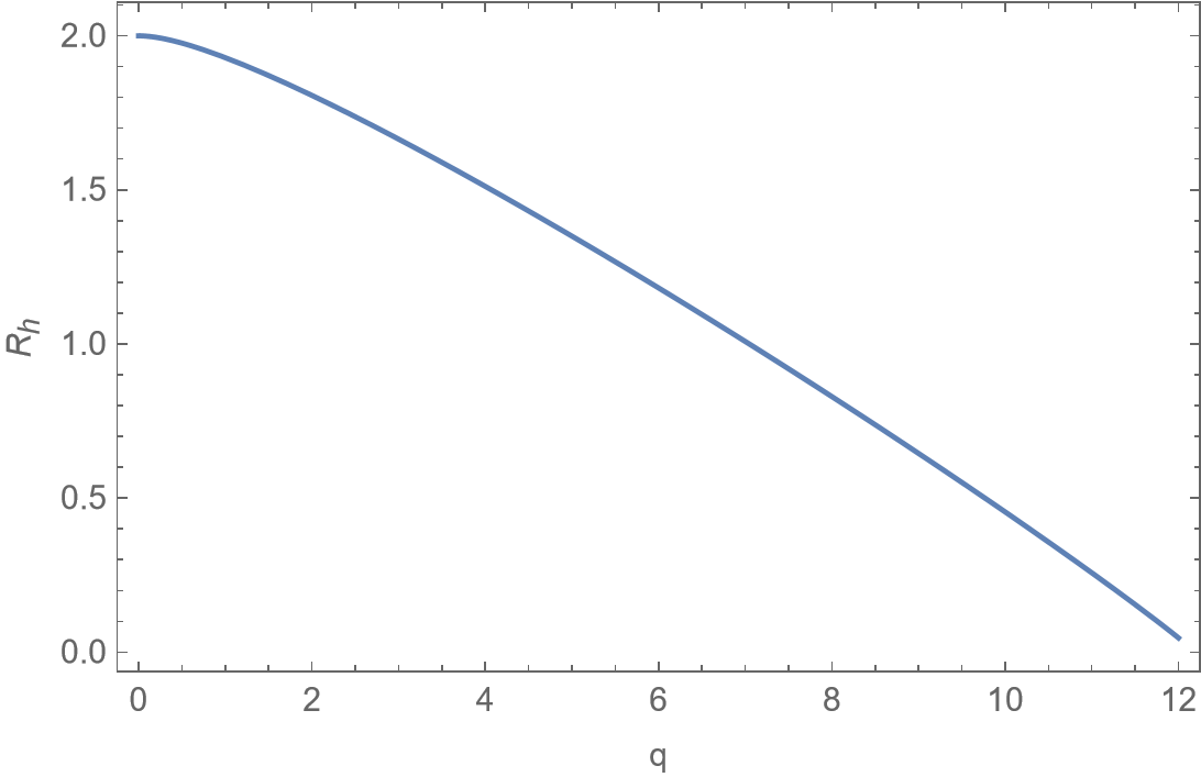
Figure 3: The black hole radius $R_{h}$ as a function of $q$. Here we set $\gamma={\textstyle{\frac{\scriptstyle 2}{\scriptstyle\sqrt{3}}}}+1$, $M=1$.

In the black hole case, the black hole mass $M$ as a function of the physical radius $R$ with different parameters are displayed in Fig. 2. The two plots of the first row are the cases that fixing $\alpha$ and varying $\gamma$. The left one with $\alpha=0.2$ and $\gamma=({\textstyle{\frac{\scriptstyle\sqrt{3}}{\scriptstyle 2}}}+0.1,{\textstyle{\frac{\scriptstyle\sqrt{3}}{\scriptstyle 2}}}+0.5,{\textstyle{\frac{\scriptstyle\sqrt{3}}{\scriptstyle 2}}}+1)$ correspond to the blue lines from top to down, respectively. The right one with $\alpha=-1$ and $\gamma=({\textstyle{\frac{\scriptstyle\sqrt{3}}{\scriptstyle 2}}}+0.01,{\textstyle{\frac{\scriptstyle\sqrt{3}}{\scriptstyle 2}}}+0.03,{\textstyle{\frac{\scriptstyle\sqrt{3}}{\scriptstyle 2}}}+0.1)$ correspond to the blue lines from top to down, respectively. The two plots of the second row are the cases that fixing $\gamma$ and varying $\alpha$. The left one with $\gamma={\textstyle{\frac{\scriptstyle\sqrt{3}}{\scriptstyle 2}}}+0.5$ and $\alpha=(0.3,0.5,1.2)$ correspond to the blue lines from top to down, respectively. The right one with $\gamma={\textstyle{\frac{\scriptstyle\sqrt{3}}{\scriptstyle 2}}}-0.05$ and $\alpha=(-0.3,-0.5,-1.2)$ correspond to the blue lines from top to down, respectively. It is obvious, in a fixed theory, that light black holes have significant deviations from the standard Schwarzschild black hole. To be specific, the hairy black holes possess smaller radii than the same mass Schwarzschild black holes. It follows that the scalar field causes the black holes more compact. A natural question comes to us: how is the smallest hairy black hole we have in this theory?

To address this question, it is convenient take $\alpha={\textstyle{\frac{\scriptstyle 3(1+q\sqrt{\gamma^{2}-1})}{\scriptstyle 2q^{3}\gamma^{2}\sqrt{\gamma^{2}-1}(3\gamma^{2}-4)}}}$, i.e. fixing the black hole mass $M=1$. The black hole condition requires $0<q<3(\gamma+\sqrt{\gamma^{2}-1})$. We display the hairy black hole radii as a function of $q$ in Fig. 3. One can see that the black hole radius tends to $2M$ when $q\to 0$, and tends to $0$ when $q\to 3(\gamma+\sqrt{\gamma^{2}-1})$. It shows that these hairy black holes are always smaller than the standard Schwarzschild black hole and could have infinitesimal areas. The small area, even zero area black holes also arise in string theories [94] and other discussions [95, 96, 97].

4 Energy conditions

The no-scalar hair theorem states that it is impossible to implement scalar hairs to the black holes in some conditions (see details in a very good review in Ref.[74]). We obtained it with a specific scalar potential that violates the weak energy condition.

Interestingly, not all the energy conditions are violated. We examine the null energy condition (NEC) as a warm up. The NEC states that, for any null vector $k^{\mu}$, $k^{\mu}k^{\nu}T_{\mu\nu}\geq 0$. With the help of (6), the contraction gives rise to

$$k^{\mu}k^{\nu}T_{\mu\nu}={\textstyle{\frac{\scriptstyle 1}{\scriptstyle 2}}}(k^{\mu}\partial_{\mu}\phi)^{2}\geq 0.$$ (13)

It means the scalar potential will not affect the NEC. It shows the fact that the normal kinetic term of scalar field is satisfied NEC. Hence our solution doesn’t violate NEC, that is some kind of trivial.

As for the weak energy condition (WEC), namely for any time-like vector $\xi^{\mu}$, it requires $\xi^{\mu}\xi^{\nu}T_{\mu\nu}\geq 0$. With the condition $\xi^{\mu}\xi_{\mu}=-1$, we have

$$\xi^{\mu}\xi^{\nu}T_{\mu\nu}={\frac{1}{2}}(\xi^{\mu}\partial_{\mu}\phi)^{2}+{\frac{1}{4}}(\partial\phi)^{2}+{\frac{1}{2}}V.$$ (14)

The inner product of $(\xi^{\mu}\partial_{\mu}\phi)^{2}$ is always positive, so the weak energy condition is determined by the last two terms of (14). We found that WEC is always violated in the vicinity of the black hole horizon. However, the results are always positive for the naked singularity solutions and hence respect the WEC. For instance, we plot the WEC for black holes and naked singularities in Fig.4.

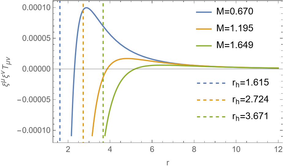
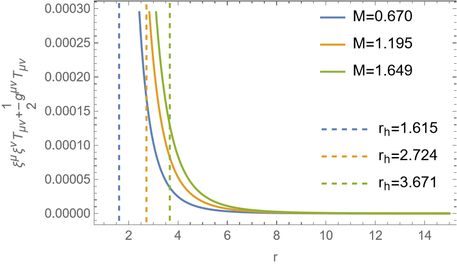
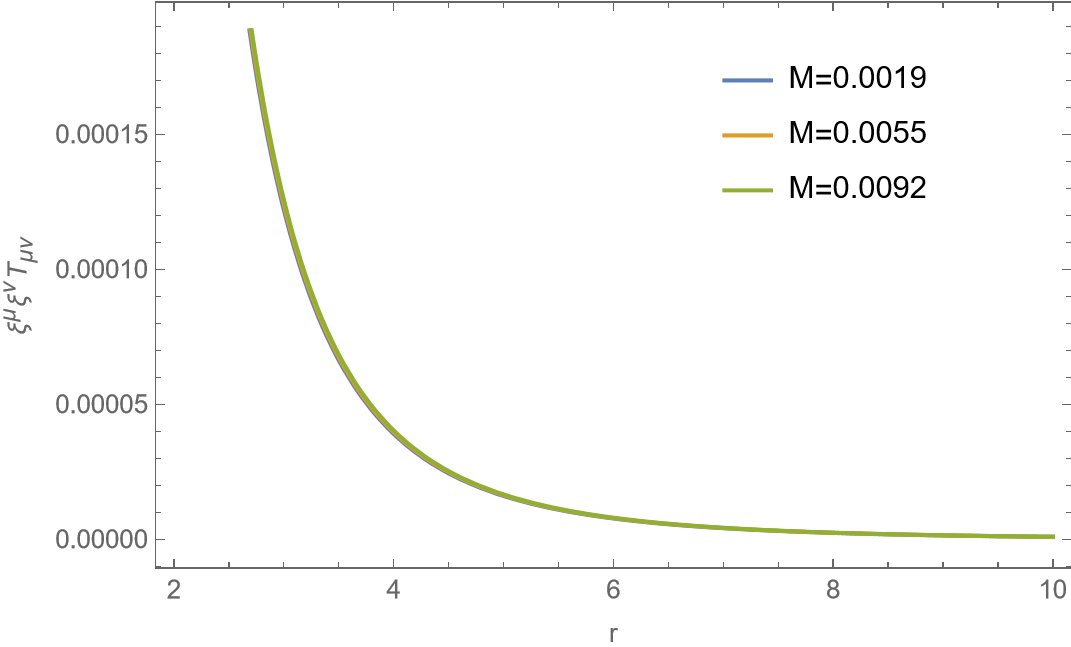
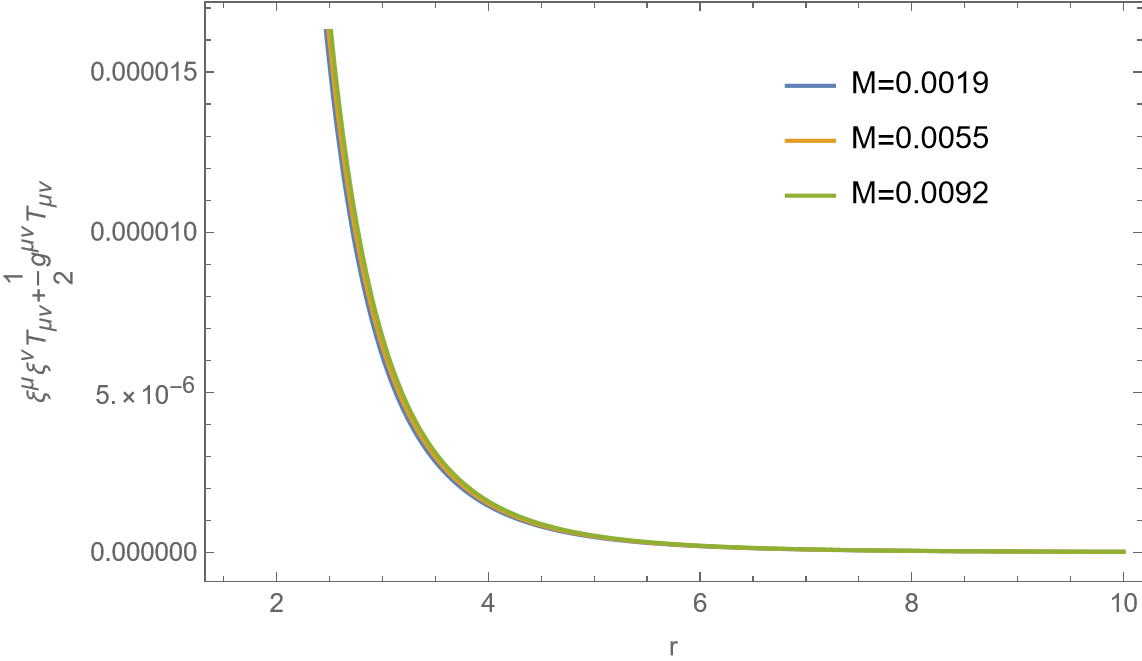
Figure 4: the SEC and WEC condition for the naked singularities and the black hole investigated with $\gamma=2$, $\alpha=-\beta=4.555$. The first two figures above are black holes, while the last two figures are naked singularities.

The strong energy condition (SEC) should also be checked, which states that

$$\xi^{\mu}\xi^{\nu}T_{\mu\nu}+{\frac{1}{2}}g^{\mu\nu}T_{\mu\nu}\geq 0,$$ (15)

for any time-like vector $\xi^{\mu}$. In the framework of our theory, the SEC condition equals to

$${\frac{1}{2}}(\xi^{\mu}\partial_{\mu}\phi)^{2}-{\frac{1}{2}}V\geq 0.$$ (16)

Since $V$ is negative, the SEC is always held. We show an example of SEC in Fig.4.

We may therefore conclude that the naked singularities respect all three energy conditions while the black holes do not.

5 Quasinormal modes

Quasinormal modes (QNMs) play an essential role in the black hole perturbation theory. It is a powerful tool to distinguish the gravitational waves emitted by binaries by comparing the QNMs in the ringdown stage. QNMs of black holes are pivotal in unraveling the properties of black holes and gravitational phenomena in the universe. QNMs have complex frequencies, where the real part signifies the oscillation frequency—the inherent rate at which perturbations oscillate around the black hole. Meanwhile, the imaginary part denotes the decay rate, indicating how rapidly the perturbations weaken over time. We would like to investigate the differences between the Schwarzschild black hole and our hairy black hole in this section.

From the theoretical prospects, there are two common perspectives to the black hole perturbations: by imposing an additional test field to the black hole background or perturbing the metric directly[98]. Due to our motivation being mainly to give a qualitative explanation for the time evolution, we take the previous viewpoint and consider only a free scalar as the test field. Furthermore, the fundamental mode is considered in the rest work.

There are many methods to calculate QNMs, including the WKB approximation method[99, 100, 102, 101], the asymptotic iteration method(AIM)[103], the spectral method[104, 105, 106, 107, 108], the finite difference method [109, 110, 111, 112], and so on. We adopt the time-evolution method by numerically solving the E.O.Ms and use the Pronny method to extract the QNM’s frequencies.

5.1 Test field and the effective potential

We consider a massless scalar as the test field, in the black hole background. The E.O.M of the scalar field is

$$\Box\psi={\frac{1}{\sqrt{-g}}}\partial_{\mu}\bigg{(}\sqrt{-g}g^{\mu\nu}\partial_{\nu}\psi(t,r,\theta,\varphi)\bigg{)}=0.$$ (17)

As a static and spherically space-time, we can separate the scalar field $\psi$ into spherical harmonics $Y_{lm}$ and radial part $\Phi(t,r)$, namely

$$\ \psi(t,r,\theta,\varphi)=\sum_{l,m}{\frac{\Phi(t,r)}{R(r)}}Y_{lm}(\theta,\varphi).$$ (18)

Thus, the above equation (17) reduces to

$$-{\frac{\partial^{2}\Phi(t,r)}{\partial t^{2}}}+hf{\frac{\partial^{2}\Phi(t,r)}{\partial r^{2}}}+{\frac{1}{2}}(fh^{\prime}+hf^{\prime}){\frac{\partial\Phi(t,r)}{\partial r}}-V(r)\Phi(t,r)=0,$$ (19)

with the effective potential

$$V(r)={\frac{l(l+1)}{R^{2}}}h+{\frac{1}{2R}}R^{\prime}(hf)^{\prime}+{\frac{hfR^{\prime\prime}}{R}}.$$ (20)

The tortoise coordinate $r_{*}$ is employed by the transformation

$$dr_{*}={\frac{dr}{\sqrt{hf}}}.$$ (21)

With the help of tortoise coordinate, one can map the radial region from $r\in(r_{h},+\infty)$ to $r_{*}\in(-\infty,+\infty)$. The scalar field equation (19) reduce to a Schrödinger-like equation

$$-{\frac{\partial^{2}\Phi(t,r)}{\partial t^{2}}}+{\frac{\partial^{2}\Phi(t,r)}{\partial r_{*}^{2}}}-V(r)\Phi(t,r)=0.$$ (22)

Before we perform the numerical algorithm to solve the equation (22), it is important to analyze the behaviors of the effective potential (20) of the hairy black holes. It always exhibits a single peak, similar to other typical black holes. We present some examples of the effective potential in Fig.5. The effective potential is zero at the event horizon, then ascends to reach a peak, and subsequently diminishes, indicating distinct behavior in quasinormal modes (QNMs). And, the peak of the hairy black hole’s potential increases with the angular number $l$, while shifting to the right, resembling the characteristics of a Schwarzschild black hole. Furthermore, the dependence of the hairy black hole on the angular number $l$ is similar to that of the Schwarzschild black hole.

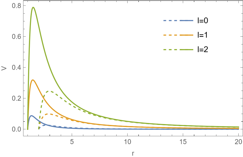
Figure 5: Effective potentials for various values of angular momentum. The dashed line corresponds to Schwarzschild black hole and the solid line to the hairy black hole. We set $\gamma={\textstyle{\frac{\scriptstyle 2}{\scriptstyle\sqrt{3}}}}+1$, $M=1$, $q=7$.

Nonetheless, one of the distinctions between this hairy black hole and the Schwarzschild black hole is the high of peaks in the effective potential for the hairy black hole is greater than that of the Schwarzschild black hole for the same angular momentum parameter. This feature affects the oscillated frequencies and the damping times in their QNMs.

5.2 Time domain integration

Now we used the Finite difference method to solve the Schrödinger-like wave equation. To begin with, we discretize the coordinates $t=i\Delta t$ and $r_{*}=i\Delta r_{*}$, then the equation (22) becomes

$$-{\frac{\Phi(i+1,j)-2\Phi(i,j)+\Phi(i-1,j)}{\Delta t^{2}}}+{\frac{\Phi(i,j+1)-2\Phi(i,j)+\Phi(i,j-1)}{\Delta r_{*}^{2}}}-V(j)\Phi(i,j)=0.$$ (23)

The initial condition that we used is the Gaussian distribution [114]

$$\begin{cases}&\Phi(t=0,r_{*})=e^{-{\frac{(r_{*}-a)^{2}}{2b^{2}}}},\\ &\Phi(t<0,r_{*})=0,\end{cases}$$ (24)

choosing $b=1$ and determining the value of a accordingly in this work. Consequently, the equation of $\Phi$ reduces to

$$\Phi(i+1,j)=-\Phi(i-1,j)+\bigg{(}2-2{\frac{\Delta t^{2}}{\Delta r_{*}^{2}}}-\Delta t^{2}V(j)\bigg{)}\Phi(i,j)+{\frac{\Delta t^{2}}{\Delta r_{*}^{2}}}\bigg{(}\Phi(i,j+1)+\Phi(i,j-1)\bigg{)}\,.$$ (25)

Inherently, solving the above equation requires appropriate boundary conditions. In black hole background, there are only ingoing waves at the horizon and outgoing waves at the infinity. It implies that the boundary conditions are

$$\partial_{t}\Phi=\pm\partial_{r_{*}}\Phi,\qquad\text{for}\quad r_{*}\to\pm\infty.$$ (26)

We take ${\textstyle{\frac{\scriptstyle\Delta t}{\scriptstyle\Delta r_{*}}}}=0.5$ to satisfy the von Neumann stability condition, which requires ${\textstyle{\frac{\scriptstyle\Delta t}{\scriptstyle\Delta r_{*}}}}<1$.

We present the time-domain plots for the Schwarzschild black hole and the hairy black hole in Fig.6 and Fig.7. The time-domain plots tell us the black holes remain stable under the influence of a massless scalar field. Both the hairy black hole and the Schwarzschild black hole exhibit a decelerated decay rate as the angular number $l$ increases. Furthermore, when considering a fixed angular number $l$, the hairy black hole with a smaller black hole radius displays a faster decay rate compared to the Schwarzschild black hole in Fig.6. This suggests that the black hole radius plays a significant role in the long-term behavior and characteristics of these black holes.

Fig.7 presents the variation of the frequencies of hairy black holes with respect to the angular number under the same set of parameters. Moreover, it shows the variation of hairy black holes with respect to the black hole radius for $l=2$. The time-domain plot for $l=2$ is also included as it plays a dominant role in the ringdown signals of gravitational waves. We found the decay is observed to decelerate further with an increase in both $l$ and $R_{h}$.

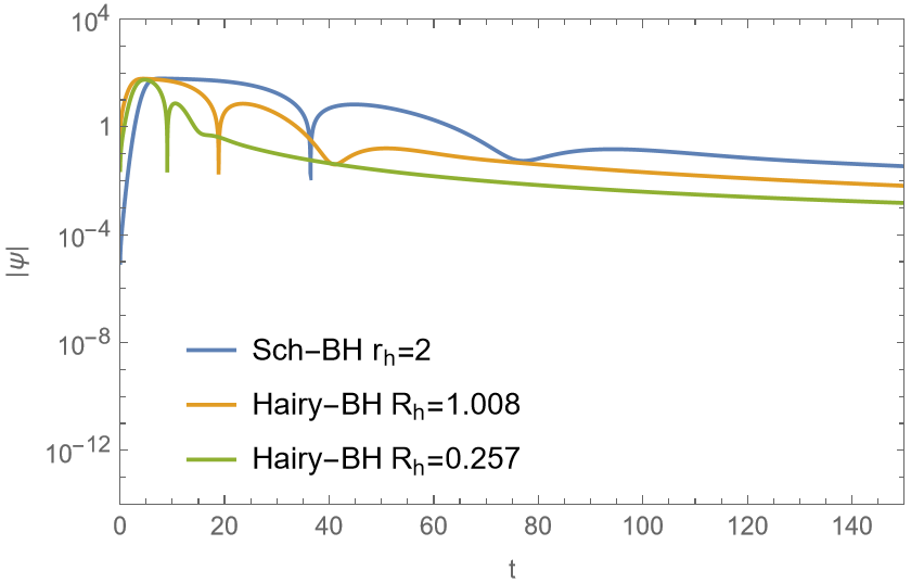
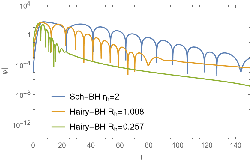
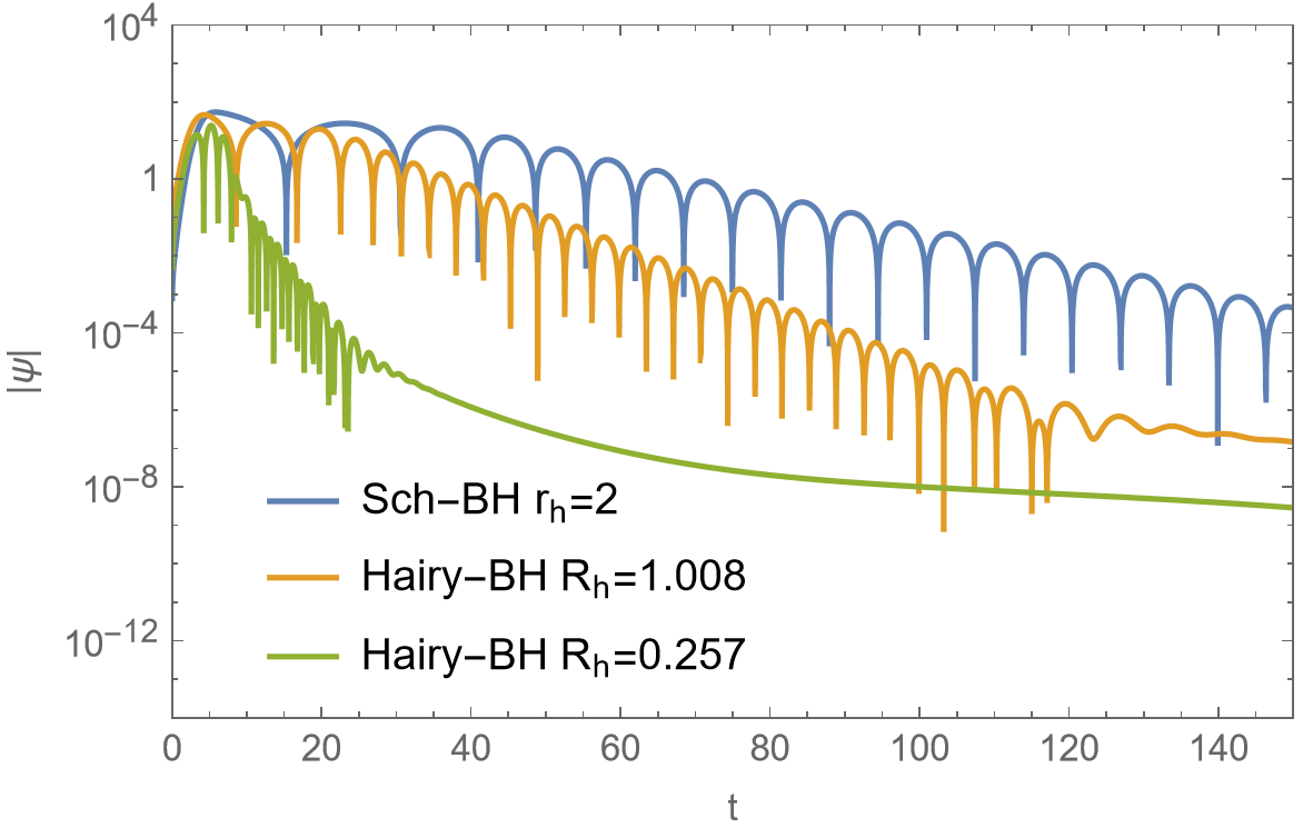
Figure 6: Time-domain plots for the Schwarzschild black hole and the hairy black hole. The left plot corresponds to $l=0$, the middle one to $l=1$, and the right one to $l=2$. Here, we take $\gamma={\textstyle{\frac{\scriptstyle 2}{\scriptstyle\sqrt{3}}}}+1$, $M=1$.

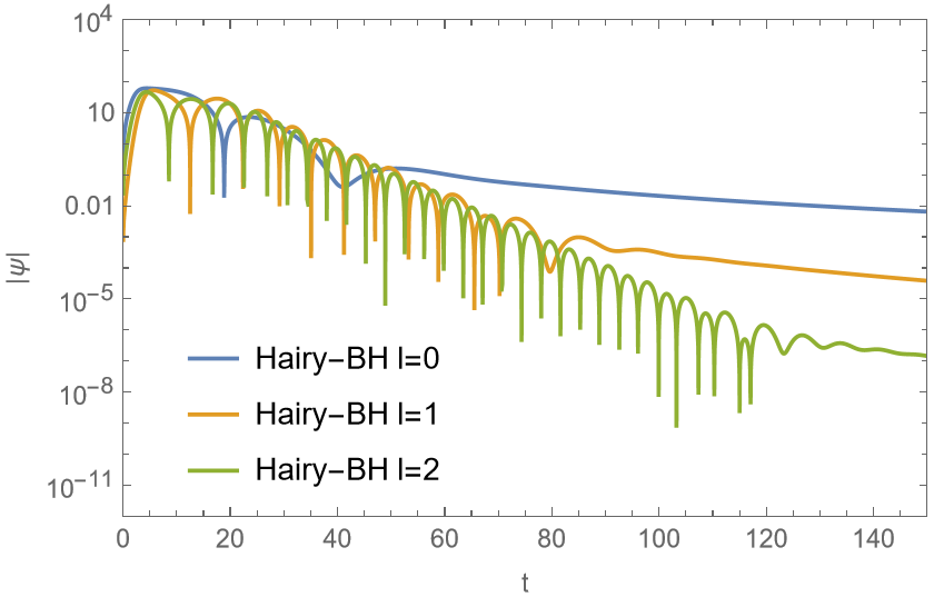
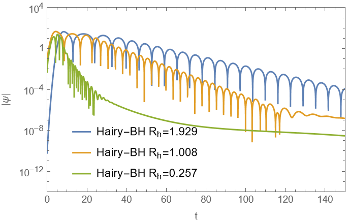
Figure 7: Time-domain plots for the hairy black hole. The left plot corresponds to $R_{h}=1.008$, and the right plot corresponds to $l=2$. Here, we take $\gamma={\textstyle{\frac{\scriptstyle 2}{\scriptstyle\sqrt{3}}}}+1$, $M=1$.

5.3 QNM’s frequencies

It is a standard method to use the Pronny Method to extract the QNM’s frequencies. We compared the QNM’s frequencies of our obtained Schwarzschild black holes with those from previous studies in Ref.[113] and found that we were able to achieve precision up to the second decimal place. This demonstrates the effectiveness of our computational method. We focused primarily on the variations of the real and imaginary parts of the frequency with respect to the horizon $R_{h}$ for the hairy black hole, as well as the variations of these parts with respect to horizon $R_{h}$ for different angular number $l$.

In detail, the new hairy black hole with $l=1,2$ are shown in Table.1. A larger real part implies a higher oscillation frequency, while a larger imaginary part indicates faster decay and a quicker disappearance of perturbations. The data in the table reveals a notable trend: as the black hole radius $R_{h}$ increases, the real part of its frequency decreases, indicating that the larger black hole radius is more effective in suppressing oscillations. Furthermore, the imaginary part of the frequency also decreases with an increase of black hole radius, meaning decaying more slowly and providing evidence for the black hole’s stability under external perturbations. Besides, the standard Schwarzschild black hole radius is always bigger than the hairy black hole with the same mass, so hairy black holes have higher oscillation frequency and decay faster. These findings align with the conclusions drawn from the previous time-domain analysis.

$R_{h}$	$l=1$	$l=2$	$l=3$
0.512	0.980555 -0.329293i	1.615452 -0.325563i	2.248509 -0.320262i
1.018	0.526765 -0.173979i	0.862807 -0.172580i	1.206043 -0.172277i
1.511	0.366889 -0.121971i	0.601491 -0.120219i	0.841138 -0.120160i
2$(Sch)$	0.293421 -0.097667i	0.483155 -0.096735i	0.675133 -0.096580i

Table 1: The quasinormal modes of the scalar field in the hairy black hole and Schwarzschild black hole. Here we set $\gamma={\textstyle{\frac{\scriptstyle 2}{\scriptstyle\sqrt{3}}}}+1$, $M=1$.

6 Conclusions

The black hole no-hair theorem has ruled out black holes with scalar hair in Einstein’s gravity with certain conditions. However, one can bypass the theorem to find out more black hole solutions by diving into modified gravities or by ignoring the conditions of the theorem. We obtained such hairy black hole solutions in the latter scheme, namely got solutions in the Einstein-scalar theory. We found these solutions can be asymptotic to Minkowski, (A)dS spacetimes, depending on the effective cosmological constant $\Lambda$.

To the interests of astrophysics, we work on the details of the asymptotic Minkowski solutions only. As we showed in the paper, the solution can depict single-horizon black holes or time-like naked singularities. This implies the solution is not a simple generalization of Schwarzschild metric. In fact, it can’t reduce Schwarzschild metric smoothly by taking $q\to 0$. Furthermore, we found the hairy black holes can possess arbitrary small areas, and their areas are always smaller than the same mass Schwarzschild black holes.

We examined the energy conditions of the hairy black holes and found they violate only the weak energy condition but respect the null and strong energy conditions. In contrast, the time-like naked singularities respect all three energy conditions.

As a hairy black hole with a single horizon, it is an interesting direction to do the comparison with Schwarzschild black hole. We considered a test scalar field in the black hole background and evaluated its time evolutions, which gives rise to the QNMs. We compared the QNM’s frequencies between the hairy black hole and Schwarzschild black hole with the same mass. The results suggest that, even the tendencies are quantitively similar, one can still distinguish the hairy black holes by its QNMs. In fact, the hairy black holes have smaller areas compared with the same mass Schwarzschild black hole, which leads to higher oscillation frequencies and shorter decay times.

We did not investigate the asymptotic (A)dS hairy black holes in this work. Based on the importance of the non-asymptotic flat black holes in theoretical studies, it deserves further studies. For future works, one can also generalize the solution to the rotation one. It has the potential to show more differences between hairy black holes with normal black holes. Our solution also provides an analytical example to the applications of black hole physics.

Appendix A

In this appendix, we present how to obtain the theory by a disformal transformation of an Einstein-phantom scalar theory in Ref.[1].

A trick we used is noting that the following transformation of metric

$$g_{\mu\nu}\to Kg_{\mu\nu},$$ (27)

with $K$ is constant, leads to

$$\sqrt{-g} \to K^{2}\sqrt{-g}\,,$$

$$(\partial\phi)^{2} \to K^{-1}(\partial\phi)^{2}\,,$$

$$R \to R\,,$$

$$V \to V.$$ (28)

Then the Lagrangian (1) becomes

$${\cal L}=K^{2}{\cal L},$$ (29)

which do not change the E.O.Ms. For our purpose, we take

$$K=e^{-\sqrt{\gamma^{2}-1}{\frac{i\pi}{\gamma}}}.$$ (30)

Together with the identity $\arctan x=i\text{arctanh}{\textstyle{\frac{\scriptstyle i}{\scriptstyle x}}}+{\textstyle{\frac{\scriptstyle\pi}{\scriptstyle 2}}}$, we therefor obtain the new scalar potential and normal scalar

$$V = e^{-\sqrt{\gamma^{2}-1}\phi}\alpha\bigg{(}(2-3\gamma^{2})\text{cosh}(\gamma\phi)-3\gamma\sqrt{\gamma^{2}-1}\text{sinh}(\gamma\phi)-2\bigg{)}$$

$$-e^{\sqrt{\gamma^{2}-1}\phi}\beta\bigg{(}-(2-3\gamma^{2})\text{cosh}(\gamma\phi)-3\gamma\sqrt{\gamma^{2}-1}\text{sinh}(\gamma\phi)+2\bigg{)},$$

$$\phi = {\frac{2}{\gamma}}\text{arctanh}({\frac{q\gamma}{\sqrt{r^{2}+q^{2}\gamma^{2}}}}).$$ (31)

By applying the corresponding transformation to the metric function, one can obtain the black hole solution that we presented in (2).

References

- [1] H. Huang, H. Lü and J. Yang, “Bronnikov-like wormholes in Einstein-scalar gravity,” Class. Quant. Grav. 39, no.18, 185009 (2022) doi:10.1088/1361-6382/ac8266 [arXiv:2010.00197 [gr-qc]].
- [2] K. Akiyama et al. [Event Horizon Telescope], “First M87 Event Horizon Telescope Results. I. The Shadow of the Supermassive Black Hole,” Astrophys. J. Lett. 875, L1 (2019)
- [3] K. Akiyama et al. [Event Horizon Telescope], “First Sagittarius A* Event Horizon Telescope Results. I. The Shadow of the Supermassive Black Hole in the Center of the Milky Way,” Astrophys. J. Lett. 930, L12 (2022)
- [4] B. P. Abbott et al. [LIGO Scientific and Virgo], “Observation of Gravitational Waves from a Binary Black Hole Merger,” Phys. Rev. Lett. 116, 061102 (2016)
- [5] H. Luck, “The GEO-600 project,” Class. Quant. Grav. 14, 1471-1476 (1997) doi:10.1088/0264-9381/14/6/012
- [6] E. Berti, V. Cardoso and C. M. Will, “On gravitational-wave spectroscopy of massive black holes with the space interferometer LISA,” Phys. Rev. D 73, 064030 (2006) doi:10.1103/PhysRevD.73.064030 [arXiv:gr-qc/0512160 [gr-qc]].
- [7] K. Somiya [KAGRA], “Detector configuration of KAGRA: The Japanese cryogenic gravitational-wave detector,” Class. Quant. Grav. 29, 124007 (2012) doi:10.1088/0264-9381/29/12/124007 [arXiv:1111.7185 [gr-qc]].
- [8] B. P. Abbott et al. [KAGRA, LIGO Scientific, Virgo and VIRGO], “Prospects for observing and localizing gravitational-wave transients with Advanced LIGO, Advanced Virgo and KAGRA,” Living Rev. Rel. 21, no.1, 3 (2018) doi:10.1007/s41114-020-00026-9 [arXiv:1304.0670 [gr-qc]].
- [9] C. Caprini, M. Chala, G. C. Dorsch, M. Hindmarsh, S. J. Huber, T. Konstandin, J. Kozaczuk, G. Nardini, J. M. No and K. Rummukainen, et al. “Detecting gravitational waves from cosmological phase transitions with LISA: an update,” JCAP 03, 024 (2020) doi:10.1088/1475-7516/2020/03/024 [arXiv:1910.13125 [astro-ph.CO]].
- [10] J. Luo et al. [TianQin], “TianQin: a space-borne gravitational wave detector,” Class. Quant. Grav. 33, no.3, 035010 (2016) doi:10.1088/0264-9381/33/3/035010 [arXiv:1512.02076 [astro-ph.IM]].
- [11] W. R. Hu and Y. L. Wu, “The Taiji Program in Space for gravitational wave physics and the nature of gravity,” Natl. Sci. Rev. 4, no.5, 685-686 (2017) doi:10.1093/nsr/nwx116
- [12] W. H. Ruan, C. Liu, Z. K. Guo, Y. L. Wu and R. G. Cai, “The LISA-Taiji network,” Nature Astron. 4, 108-109 (2020) doi:10.1038/s41550-019-1008-4 [arXiv:2002.03603 [gr-qc]].
- [13] S. J. Huang, Y. M. Hu, V. Korol, P. C. Li, Z. C. Liang, Y. Lu, H. T. Wang, S. Yu and J. Mei, “Science with the TianQin Observatory: Preliminary results on Galactic double white dwarf binaries,” Phys. Rev. D 102, no.6, 063021 (2020) doi:10.1103/PhysRevD.102.063021 [arXiv:2005.07889 [astro-ph.HE]].
- [14] W. Israel, “Event horizons in static vacuum space-times,” Phys. Rev. 164, 1776-1779 (1967) doi:10.1103/PhysRev.164.1776
- [15] D. C. Robinson, “Uniqueness of the Kerr black hole,” Phys. Rev. Lett. 34, 905-906 (1975) doi:10.1103/PhysRevLett.34.905
- [16] J. D. Bekenstein, “Black hole hair: 25 - years after,” [arXiv:gr-qc/9605059 [gr-qc]].
- [17] V. Cardoso and L. Gualtieri, “Testing the black hole ‘no-hair’ hypothesis,” Class. Quant. Grav. 33, no.17, 174001 (2016) doi:10.1088/0264-9381/33/17/174001 [arXiv:1607.03133 [gr-qc]].
- [18] J. Yang, “Novel topological black holes from thermodynamics and deforming horizons,” [arXiv:2301.01709 [gr-qc]].
- [19] P. V. P. Cunha, C. A. R. Herdeiro, E. Radu and H. F. Runarsson, “Shadows of Kerr black holes with scalar hair,” Phys. Rev. Lett. 115, no.21, 211102 (2015) doi:10.1103/PhysRevLett.115.211102 [arXiv:1509.00021 [gr-qc]].
- [20] M. Khodadi, A. Allahyari, S. Vagnozzi and D. F. Mota, “Black holes with scalar hair in light of the Event Horizon Telescope,” JCAP 09, 026 (2020) doi:10.1088/1475-7516/2020/09/026 [arXiv:2005.05992 [gr-qc]].
- [21] M. Afrin, R. Kumar and S. G. Ghosh, “Parameter estimation of hairy Kerr black holes from its shadow and constraints from M87*,” Mon. Not. Roy. Astron. Soc. 504, 5927-5940 (2021) doi:10.1093/mnras/stab1260 [arXiv:2103.11417 [gr-qc]].
- [22] S. Vagnozzi, R. Roy, Y. D. Tsai, L. Visinelli, M. Afrin, A. Allahyari, P. Bambhaniya, D. Dey, S. G. Ghosh and P. S. Joshi, et al. “Horizon-scale tests of gravity theories and fundamental physics from the Event Horizon Telescope image of Sagittarius A,” Class. Quant. Grav. 40, no.16, 165007 (2023) doi:10.1088/1361-6382/acd97b [arXiv:2205.07787 [gr-qc]].
- [23] M. Khodadi, G. Lambiase and D. F. Mota, “No-hair theorem in the wake of Event Horizon Telescope,” JCAP 09, 028 (2021) doi:10.1088/1475-7516/2021/09/028 [arXiv:2107.00834 [gr-qc]].
- [24] S. Li, W. B. Han and S. C. Yang, “Tests of no-hair theorem with binary black-hole coalescences,” [arXiv:2312.02841 [gr-qc]].
- [25] S. Gossan, J. Veitch and B. S. Sathyaprakash, “Bayesian model selection for testing the no-hair theorem with black hole ringdowns,” Phys. Rev. D 85, 124056 (2012) doi:10.1103/PhysRevD.85.124056 [arXiv:1111.5819 [gr-qc]].
- [26] L. Sampson, N. Yunes, N. Cornish, M. Ponce, E. Barausse, A. Klein, C. Palenzuela and L. Lehner, “Projected Constraints on Scalarization with Gravitational Waves from Neutron Star Binaries,” Phys. Rev. D 90, no.12, 124091 (2014) doi:10.1103/PhysRevD.90.124091 [arXiv:1407.7038 [gr-qc]].
- [27] M. Isi, M. Giesler, W. M. Farr, M. A. Scheel and S. A. Teukolsky, “Testing the no-hair theorem with GW150914,” Phys. Rev. Lett. 123, no.11, 111102 (2019) doi:10.1103/PhysRevLett.123.111102 [arXiv:1905.00869 [gr-qc]].
- [28] S. Bhagwat, X. J. Forteza, P. Pani and V. Ferrari, “Ringdown overtones, black hole spectroscopy, and no-hair theorem tests,” Phys. Rev. D 101, no.4, 044033 (2020) doi:10.1103/PhysRevD.101.044033 [arXiv:1910.08708 [gr-qc]].
- [29] J. D. Bekenstein, “Black Holes with Scalar Charge,” Annals Phys. 91, 75-82 (1975) doi:10.1016/0003-4916(75)90279-1
- [30] P. Bizon, “Gravitating solitons and hairy black holes,” Acta Phys. Polon. B 25, 877-898 (1994) [arXiv:gr-qc/9402016 [gr-qc]].
- [31] U. Nucamendi and M. Salgado, “Scalar hairy black holes and solitons in asymptotically flat space-times,” Phys. Rev. D 68, 044026 (2003) doi:10.1103/PhysRevD.68.044026 [arXiv:gr-qc/0301062 [gr-qc]].
- [32] M. S. Volkov and D. V. Gal’tsov, “Gravitating nonAbelian solitons and black holes with Yang-Mills fields,” Phys. Rept. 319, 1-83 (1999) doi:10.1016/S0370-1573(99)00010-1 [arXiv:hep-th/9810070 [hep-th]].
- [33] E. Radu, Y. Shnir and D. H. Tchrakian, “Scalar hairy black holes and solitons in a gravitating Goldstone model,” Phys. Lett. B 703, 386-393 (2011) doi:10.1016/j.physletb.2011.08.032 [arXiv:1106.5066 [gr-qc]].
- [34] A. Anabalon, D. Astefanesei and R. Mann, “Exact asymptotically flat charged hairy black holes with a dilaton potential,” JHEP 10, 184 (2013) doi:10.1007/JHEP10(2013)184 [arXiv:1308.1693 [hep-th]].
- [35] X. H. Feng, H. Lu and Q. Wen, “Scalar Hairy Black Holes in General Dimensions,” Phys. Rev. D 89, no.4, 044014 (2014) doi:10.1103/PhysRevD.89.044014 [arXiv:1312.5374 [hep-th]].
- [36] C. A. R. Herdeiro and E. Radu, “Kerr black holes with scalar hair,” Phys. Rev. Lett. 112, 221101 (2014) doi:10.1103/PhysRevLett.112.221101 [arXiv:1403.2757 [gr-qc]].
- [37] T. P. Sotiriou and S. Y. Zhou, “Black hole hair in generalized scalar-tensor gravity: An explicit example,” Phys. Rev. D 90, 124063 (2014) doi:10.1103/PhysRevD.90.124063 [arXiv:1408.1698 [gr-qc]].
- [38] Z. Y. Fan and H. Lu, “Charged Black Holes with Scalar Hair,” JHEP 09, 060 (2015) doi:10.1007/JHEP09(2015)060 [arXiv:1507.04369 [hep-th]].
- [39] C. Herdeiro and E. Radu, “Construction and physical properties of Kerr black holes with scalar hair,” Class. Quant. Grav. 32, no.14, 144001 (2015) doi:10.1088/0264-9381/32/14/144001 [arXiv:1501.04319 [gr-qc]].
- [40] H. Luckock and I. Moss, “BLACK HOLES HAVE SKYRMION HAIR,” Phys. Lett. B 176, 341-345 (1986) doi:10.1016/0370-2693(86)90175-9
- [41] B. Kleihaus, J. Kunz and A. Sood, “Charged SU(N) Einstein Yang-Mills black holes,” Phys. Lett. B 418, 284-293 (1998) doi:10.1016/S0370-2693(97)01447-0 [arXiv:hep-th/9705179 [hep-th]].
- [42] B. Kleihaus, J. Kunz, A. Sood and M. Wirschins, “Black holes with Yang-Mills hair,” AIP Conf. Proc. 453, no.1, 478 (1998) doi:10.1063/1.57143 [arXiv:gr-qc/9807035 [gr-qc]].
- [43] B. Hartmann, B. Kleihaus and J. Kunz, “Axially symmetric monopoles and black holes in Einstein-Yang-Mills-Higgs theory,” Phys. Rev. D 65, 024027 (2002) doi:10.1103/PhysRevD.65.024027 [arXiv:hep-th/0108129 [hep-th]].
- [44] B. Kleihaus, J. Kunz and F. Navarro-Lerida, “Rotating Einstein-Yang-Mills black holes,” Phys. Rev. D 66, 104001 (2002) doi:10.1103/PhysRevD.66.104001 [arXiv:gr-qc/0207042 [gr-qc]].
- [45] R. Ibadov, B. Kleihaus, J. Kunz and M. Wirschins, “New black hole solutions with axial symmetry in Einstein-Yang-Mills theory,” Phys. Lett. B 627, 180-187 (2005) doi:10.1016/j.physletb.2005.08.108 [arXiv:gr-qc/0507110 [gr-qc]].
- [46] R. Brito, V. Cardoso and P. Pani, “Black holes with massive graviton hair,” Phys. Rev. D 88, 064006 (2013) doi:10.1103/PhysRevD.88.064006 [arXiv:1309.0818 [gr-qc]].
- [47] C. Herdeiro, E. Radu and H. Rúnarsson, “Kerr black holes with Proca hair,” Class. Quant. Grav. 33, no.15, 154001 (2016) doi:10.1088/0264-9381/33/15/154001 [arXiv:1603.02687 [gr-qc]].
- [48] Z. Y. Fan, “Black holes with vector hair,” JHEP 09, 039 (2016) doi:10.1007/JHEP09(2016)039 [arXiv:1606.00684 [hep-th]].
- [49] Y. Shnir, “Black holes with Skyrmion-anti-Skyrmion hairs,” Phys. Lett. B 810, 135847 (2020) doi:10.1016/j.physletb.2020.135847 [arXiv:2008.09452 [hep-th]].
- [50] T. Tamaki, K. i. Maeda and M. Inada, “Properties of black hole solutions in the SU(3) Einstein-Yang-Mills dilaton system,” Phys. Rev. D 63, 087504 (2001) doi:10.1103/PhysRevD.63.087504
- [51] H. Lu, C. N. Pope and Q. Wen, “Thermodynamics of AdS Black Holes in Einstein-Scalar Gravity,” JHEP 03, 165 (2015) doi:10.1007/JHEP03(2015)165 [arXiv:1408.1514 [hep-th]].
- [52] Z. Y. Fan, B. Chen and H. Lu, “Global Structure of Exact Scalar Hairy Dynamical Black Holes,” JHEP 05, 170 (2016) doi:10.1007/JHEP05(2016)170 [arXiv:1601.07246 [hep-th]].
- [53] Y. Guo and Y. G. Miao, “Scalar quasinormal modes of black holes in Einstein-Yang-Mills gravity,” Phys. Rev. D 102, no.6, 064049 (2020) doi:10.1103/PhysRevD.102.064049 [arXiv:2005.07524 [hep-th]].
- [54] E. Berti, E. Barausse, V. Cardoso, L. Gualtieri, P. Pani, U. Sperhake, L. C. Stein, N. Wex, K. Yagi and T. Baker, et al. “Testing General Relativity with Present and Future Astrophysical Observations,” Class. Quant. Grav. 32, 243001 (2015) doi:10.1088/0264-9381/32/24/243001 [arXiv:1501.07274 [gr-qc]].
- [55] L. Barack, V. Cardoso, S. Nissanke, T. P. Sotiriou, A. Askar, C. Belczynski, G. Bertone, E. Bon, D. Blas and R. Brito, et al. “Black holes, gravitational waves and fundamental physics: a roadmap,” Class. Quant. Grav. 36, no.14, 143001 (2019) doi:10.1088/1361-6382/ab0587 [arXiv:1806.05195 [gr-qc]].
- [56] D. J. Gogoi and S. Ponglertsakul, “Constraints on Quasinormal modes from Black Hole Shadows in regular non-minimal Einstein Yang-Mills Gravity,” [arXiv:2402.06186 [gr-qc]].
- [57] R. Contino, M. Ghezzi, C. Grojean, M. Muhlleitner and M. Spira, “Effective Lagrangian for a light Higgs-like scalar,” JHEP 07, 035 (2013) doi:10.1007/JHEP07(2013)035 [arXiv:1303.3876 [hep-ph]].
- [58] J. Preskill, M. B. Wise and F. Wilczek, “Cosmology of the Invisible Axion,” Phys. Lett. B 120, 127-132 (1983) doi:10.1016/0370-2693(83)90637-8
- [59] J. L. Feng, “Dark Matter Candidates from Particle Physics and Methods of Detection,” Ann. Rev. Astron. Astrophys. 48, 495-545 (2010) doi:10.1146/annurev-astro-082708-101659 [arXiv:1003.0904 [astro-ph.CO]].
- [60] G. Ballesteros, J. Redondo, A. Ringwald and C. Tamarit, “Unifying inflation with the axion, dark matter, baryogenesis and the seesaw mechanism,” Phys. Rev. Lett. 118, no.7, 071802 (2017) doi:10.1103/PhysRevLett.118.071802 [arXiv:1608.05414 [hep-ph]].
- [61] L. Hui, J. P. Ostriker, S. Tremaine and E. Witten, “Ultralight scalars as cosmological dark matter,” Phys. Rev. D 95, no.4, 043541 (2017) doi:10.1103/PhysRevD.95.043541 [arXiv:1610.08297 [astro-ph.CO]].
- [62] A. Caldwell et al. [MADMAX Working Group], “Dielectric Haloscopes: A New Way to Detect Axion Dark Matter,” Phys. Rev. Lett. 118, no.9, 091801 (2017) doi:10.1103/PhysRevLett.118.091801 [arXiv:1611.05865 [physics.ins-det]].
- [63] E. J. Copeland, M. Sami and S. Tsujikawa, “Dynamics of dark energy,” Int. J. Mod. Phys. D 15, 1753-1936 (2006) doi:10.1142/S021827180600942X [arXiv:hep-th/0603057 [hep-th]].
- [64] M. Li, X.-D. Li, S. Wang and Y. Wang, “Dark Energy,” Commun. Theor. Phys. 56, 525–604 (2011) doi:10.1088/0253-6102/56/3/24 [arXiv:1103.5870 [astro-ph.CO]].
- [65] L. Kofman, A. D. Linde and A. A. Starobinsky, “Reheating after inflation,” Phys. Rev. Lett. 73, 3195-3198 (1994) doi:10.1103/PhysRevLett.73.3195 [arXiv:hep-th/9405187 [hep-th]].
- [66] J. Martin, C. Ringeval and V. Vennin, “Encyclopædia Inflationaris” Phys. Dark Univ. 5-6, 75–235, (2014) doi:10.1016/j.dark.2014.01.003 [arXiv:1303.3787 [astro-ph.CO]].
- [67] P. Svrcek and E. Witten, “Axions In String Theory,” JHEP 06, 051 (2006) doi:10.1088/1126-6708/2006/06/051 [arXiv:hep-th/0605206 [hep-th]].
- [68] A. Arvanitaki, S. Dimopoulos, S. Dubovsky, N. Kaloper and J. March-Russell, “String Axiverse,” Phys. Rev. D 81, 123530 (2010) doi:10.1103/PhysRevD.81.123530 [arXiv:0905.4720 [hep-th]].
- [69] E. Palti, “The Swampland: Introduction and Review,” Fortsch. Phys. 67, 1900037 (2019) doi:10.1002/prop.201900037 [arXiv:1903.06239 [hep-th]].
- [70] J. D. Bekenstein, “Transcendence of the law of baryon-number conservation in black hole physics,” Phys. Rev. Lett. 28, 452-455 (1972) doi:10.1103/PhysRevLett.28.452
- [71] J. D. Bekenstein, “Nonexistence of baryon number for static black holes,” Phys. Rev. D 5, 1239-1246 (1972) doi:10.1103/PhysRevD.5.1239
- [72] J. D. Bekenstein, “Nonexistence of baryon number for black holes. ii,” Phys. Rev. D 5, 2403-2412 (1972) doi:10.1103/PhysRevD.5.2403
- [73] J. D. Bekenstein, “Novel “no-scalar-hair” theorem for black holes,” Phys. Rev. D 51, no.12, R6608 (1995) doi:10.1103/PhysRevD.51.R6608
- [74] C. A. R. Herdeiro and E. Radu, “Asymptotically flat black holes with scalar hair: a review,” Int. J. Mod. Phys. D 24, no.09, 1542014 (2015) doi:10.1142/S0218271815420146 [arXiv:1504.08209 [gr-qc]].
- [75] B. Kleihaus, J. Kunz and S. Yazadjiev, “Scalarized Hairy Black Holes,” Phys. Lett. B 744, 406-412 (2015) doi:10.1016/j.physletb.2015.04.014 [arXiv:1503.01672 [gr-qc]].
- [76] J. L. Blázquez-Salcedo, D. D. Doneva, J. Kunz and S. S. Yazadjiev, “Radial perturbations of the scalarized Einstein-Gauss-Bonnet black holes,” Phys. Rev. D 98, no.8, 084011 (2018) doi:10.1103/PhysRevD.98.084011 [arXiv:1805.05755 [gr-qc]].
- [77] E. Berti, L. G. Collodel, B. Kleihaus and J. Kunz, “Spin-induced black-hole scalarization in Einstein-scalar-Gauss-Bonnet theory,” Phys. Rev. Lett. 126, no.1, 011104 (2021) doi:10.1103/PhysRevLett.126.011104 [arXiv:2009.03905 [gr-qc]].
- [78] M. Y. Lai, Y. S. Myung, R. H. Yue and D. C. Zou, “Spin-induced scalarization of Kerr-Newman black holes in Einstein-Maxwell-scalar theory,” Phys. Rev. D 106, no.4, 044045 (2022) doi:10.1103/PhysRevD.106.044045 [arXiv:2206.11587 [gr-qc]].
- [79] M. Y. Lai, Y. S. Myung, R. H. Yue and D. C. Zou, “Spin-charge induced spontaneous scalarization of Kerr-Newman black holes,” Phys. Rev. D 106, no.8, 084043 (2022) doi:10.1103/PhysRevD.106.084043 [arXiv:2208.11849 [gr-qc]].
- [80] K. H. Fan, Y. S. Myung, D. C. Zou and M. Y. Lai, “Scalarization of Kerr-Newman black holes in the Einstein-Chern-Simons-scalar theory,” [arXiv:2401.00144 [gr-qc]].
- [81] R. Penrose, “Gravitational collapse and space-time singularities,” Phys. Rev. Lett. 14, 57-59 (1965) doi:10.1103/PhysRevLett.14.57
- [82] R. Penrose, “Gravitational collapse: The role of general relativity,” Riv. Nuovo Cim. 1, 252-276 (1969) doi:10.1023/A:1016578408204
- [83] S. W. Hawking and R. Penrose, “The Singularities of gravitational collapse and cosmology,” Proc. Roy. Soc. Lond. A 314, 529-548 (1970) doi:10.1098/rspa.1970.0021
- [84] N. Graham, “Casimir energies and general relativity energy conditions,” J. Phys. A 39, 6423-6432 (2006) doi:10.1088/0305-4470/39/21/S37 [arXiv:hep-th/0601038 [hep-th]].
- [85] J. Alexandre and D. Backhouse, “Null energy condition violation: Tunneling versus the Casimir effect,” Phys. Rev. D 107, no.8, 085022 (2023) doi:10.1103/PhysRevD.107.085022 [arXiv:2301.02455 [hep-th]].
- [86] A. G. Riess et al. [Supernova Search Team], “Observational evidence from supernovae for an accelerating universe and a cosmological constant,” Astron. J. 116, 1009-1038 (1998) doi:10.1086/300499 [arXiv:astro-ph/9805201 [astro-ph]].
- [87] S. Perlmutter et al. [Supernova Cosmology Project], “Measurements of and from 42 High Redshift Supernovae,” Astrophys. J. 517, 565-586 (1999) doi:10.1086/307221 [arXiv:astro-ph/9812133 [astro-ph]].
- [88] S. Perlmutter and B. P. Schmidt, “Measuring cosmology with supernovae,” Lect. Notes Phys. 598, 195-217 (2003) doi:10.1007/3-540-45863-8_11 [arXiv:astro-ph/0303428 [astro-ph]].
- [89] M. S. Morris and K. S. Thorne, “Wormholes in space-time and their use for interstellar travel: A tool for teaching general relativity,” Am. J. Phys. 56, 395-412 (1988) doi:10.1119/1.15620
- [90] M. S. Morris, K. S. Thorne and U. Yurtsever, “Wormholes, Time Machines, and the Weak Energy Condition,” Phys. Rev. Lett. 61, 1446-1449 (1988) doi:10.1103/PhysRevLett.61.1446
- [91] H. Huang and J. Yang, “Charged Ellis Wormhole and Black Bounce,” Phys. Rev. D 100, no.12, 124063 (2019) doi:10.1103/PhysRevD.100.124063 [arXiv:1909.04603 [gr-qc]].
- [92] J. Yang and H. Huang, “Trapping horizons of the evolving charged wormhole and black bounce,” Phys. Rev. D 104, no.8, 084005 (2021) doi:10.1103/PhysRevD.104.084005 [arXiv:2104.11134 [gr-qc]].
- [93] M. Nozawa, “Static spacetimes haunted by a phantom scalar field III: asymptotically (A)dS solutions,” Phys. Rev. D 103, no.2, 024005 (2021) doi:10.1103/PhysRevD.103.024005 [arXiv:2010.07561 [gr-qc]].
- [94] C. Chowdhury, A. Sen, P. Shanmugapriya and A. Virmani, “Supersymmetric Index for Small Black Holes,” [arXiv:2401.13730 [hep-th]].
- [95] C. F. E. Holzhey and F. Wilczek, “Black holes as elementary particles,” Nucl. Phys. B 380, 447-477 (1992) doi:10.1016/0550-3213(92)90254-9 [arXiv:hep-th/9202014 [hep-th]].
- [96] J. Preskill, P. Schwarz, A. D. Shapere, S. Trivedi and F. Wilczek, “Limitations on the statistical description of black holes,” Mod. Phys. Lett. A 6, 2353-2362 (1991) doi:10.1142/S0217732391002773
- [97] Y. Huang and H. Zhang, “True gravitational atoms: Spherical cloud of dilatonic black holes,” Phys. Rev. D 105, no.12, 124056 (2022) doi:10.1103/PhysRevD.105.124056 [arXiv:2206.05645 [gr-qc]].
- [98] R. A. Konoplya and A. Zhidenko, “Quasinormal modes of black holes: From astrophysics to string theory,” Rev. Mod. Phys. 83, 793-836 (2011) doi:10.1103/RevModPhys.83.793 [arXiv:1102.4014 [gr-qc]].
- [99] R. A. Konoplya, “Quasinormal behavior of the d-dimensional Schwarzschild black hole and higher order WKB approach,” Phys. Rev. D 68, 024018 (2003) doi:10.1103/PhysRevD.68.024018 [arXiv:gr-qc/0303052 [gr-qc]].
- [100] R. A. Konoplya, “Quasinormal modes of the Schwarzschild black hole and higher order WKB approach,” J. Phys. Stud. 8, 93-100 (2004)
- [101] J. L. Blázquez-Salcedo, X. Y. Chew and J. Kunz, “Scalar and axial quasinormal modes of massive static phantom wormholes,” Phys. Rev. D 98, no.4, 044035 (2018) doi:10.1103/PhysRevD.98.044035 [arXiv:1806.03282 [gr-qc]].
- [102] R. A. Konoplya, A. Zhidenko and A. F. Zinhailo, “Higher order WKB formula for quasinormal modes and grey-body factors: recipes for quick and accurate calculations,” Class. Quant. Grav. 36, 155002 (2019) doi:10.1088/1361-6382/ab2e25 [arXiv:1904.10333 [gr-qc]].
- [103] A. Jansen, “Overdamped modes in Schwarzschild-de Sitter and a Mathematica package for the numerical computation of quasinormal modes,” Eur. Phys. J. Plus 132, no.12, 546 (2017) doi:10.1140/epjp/i2017-11825-9 [arXiv:1709.09178 [gr-qc]].
- [104] J. L. Blázquez-Salcedo, F. S. Khoo, J. Kunz and L. M. González-Romero, “Quasinormal modes of Kerr black holes using a spectral decomposition of the metric perturbations,” [arXiv:2312.10754 [gr-qc]].
- [105] F. S. Khoo, B. Azad, J. L. Blázquez-Salcedo, L. M. González-Romero, B. Kleihaus, J. Kunz and F. Navarro-Lérida, “Quasinormal modes of rapidly rotating Ellis-Bronnikov wormholes,” [arXiv:2401.02898 [gr-qc]].
- [106] A. K. W. Chung, P. Wagle and N. Yunes, “Spectral method for the gravitational perturbations of black holes: Schwarzschild background case,” Phys. Rev. D 107, no.12, 124032 (2023) doi:10.1103/PhysRevD.107.124032 [arXiv:2302.11624 [gr-qc]].
- [107] A. K. W. Chung, P. Wagle and N. Yunes, “Spectral method for metric perturbations of black holes: Kerr background case in general relativity,” Phys. Rev. D 109, no.4, 044072 (2024) doi:10.1103/PhysRevD.109.044072 [arXiv:2312.08435 [gr-qc]].
- [108] B. Azad, J. L. Blázquez-Salcedo, F. S. Khoo and J. Kunz, “Radial perturbations of Ellis-Bronnikov wormholes in slow rotation up to second order,” [arXiv:2403.08387 [gr-qc]].
- [109] M. Y. Ou, M. Y. Lai and H. Huang, “Echoes from asymmetric wormholes and black bounce,” Eur. Phys. J. C 82, no.5, 452 (2022) doi:10.1140/epjc/s10052-022-10421-x [arXiv:2111.13890 [gr-qc]].
- [110] H. Huang, M. Y. Ou, M. Y. Lai and H. Lu, “Echoes from classical black holes,” Phys. Rev. D 105, no.10, 104049 (2022) doi:10.1103/PhysRevD.105.104049 [arXiv:2112.14780 [hep-th]].
- [111] G. Guo, P. Wang, H. Wu and H. Yang, “Quasinormal modes of black holes with multiple photon spheres,” JHEP 06, 060 (2022) doi:10.1007/JHEP06(2022)060 [arXiv:2112.14133 [gr-qc]].
- [112] G. Guo, P. Wang, H. Wu and H. Yang, “Echoes from hairy black holes,” JHEP 06, 073 (2022) doi:10.1007/JHEP06(2022)073 [arXiv:2204.00982 [gr-qc]].
- [113] R. A. Konoplya and A. Zhidenko, “Analytic expressions for quasinormal modes and grey-body factors in the eikonal limit and beyond,” Class. Quant. Grav. 40, no.24, 245005 (2023) doi:10.1088/1361-6382/ad0a52 [arXiv:2309.02560 [gr-qc]].
- [114] H. Liu, P. Liu, Y. Liu, B. Wang and J. P. Wu, “Echoes from phantom wormholes,” Phys. Rev. D 103, no.2, 024006 (2021) doi:10.1103/PhysRevD.103.024006 [arXiv:2007.09078 [gr-qc]].