Multiple testing in game-theoretic probability: pictures and questions
Abstract
The usual way of testing probability forecasts in game-theoretic probability is via construction of test martingales. The standard assumption is that all forecasts are output by the same forecaster. In this paper I will discuss possible extensions of this picture to testing probability forecasts output by several forecasters. This corresponds to multiple hypothesis testing in statistics. One interesting phenomenon is that even a slight relaxation of the requirement of family-wise validity leads to a very significant increase in the efficiency of testing procedures. The main goal of this paper is to report results of preliminary simulation studies and list some directions of further research.
The version of this paper at http://alrw.net/e (Working Paper 10) is updated most often.
1 Introduction
Game-theoretic probability, as presented in, e.g., my joint books [11] and [12] with Glenn Shafer, is based on the idea that a null hypothesis can be tested dynamically by gambling against it. More generally, we are testing a player called Forecaster, which can be a scientific theory, a computer program, a human forecaster, etc. The gambler starts from an initial capital of 1 and is required to keep his capital nonnegative. His current capital is interpreted as the degree to which the null hypothesis has been undermined.
The idea of testing via gambling goes back at least to Richard von Mises’s principle of the impossibility of a gambling system (Unmöglichkeit eines Spielsystems [14, p. 58]), but von Mises’s notion of gambling was too narrow, and it was only applicable to infinite sequences. The narrowness of von Mises’s notion of gambling was demonstrated by Ville [13, Sect. II.4] (for an English translation, see [9]). Ville proposed extending von Mises’s testing procedure to using nonnegative martingales [13, Chap. IV], but somewhat surprisingly, did not explicitly apply his wider notion of testing to restate von Mises’s principle of the impossibility of a gambling system. It appears that the idea of testing using nonnegative martingales emerged gradually in various fields, including the algorithmic theory of randomness.
In this paper we will be interested in testing several forecasters in one go, with different forecasters being tested at different steps. Testing by gambling can be studied in the usual setting of measure-theoretic probability, and this is what we will do in this paper, for simplicity and as a first step. Replacing measure-theoretic probability by game-theoretic probability as mathematical foundation for our definitions and results will be one of directions of future research. For now, each forecaster will be formalized as a composite null hypothesis, represented by a set of probability measures on the sample space.
In principle, we can consider two settings for testing multiple null hypotheses. In the closed setting, we have a fixed number of null hypotheses. In the open setting, the number of null hypotheses is not known in advance and is potentially infinite. In this paper we will concentrate on the closed setting.
This paper has been prepared in support of my planned talk at the Oberwolfach workshop “Game-theoretic statistical inference: optional sampling, universal inference, and multiple testing based on e-values” organized by Peter Grünwald, Aaditya Ramdas, Ruodu Wang, and Johanna Ziegel (5–10 May 2024).
2 Dynamic necessity and possibility
Let us fix a probability space equipped with a filtration , so that is a nested sequence of -algebras. Apart from the true probability measure we will often consider other probability measures on the measurable space . Our notation for the expectation of a random variable w.r. to will be , abbreviated to when (in general, “w.r. to ” or the indication of is usually omitted when ). Let be the family of all probability measures on .
A test martingale w.r. to is a sequence of random variables taking values in such that and for all . A martingale test is a family of test martingales w.r. to . At each time , we interpret as a measure of disagreement between the realized outcome and its putative explanation ; we may say that is -strange at time w.r. to if .
Fix a martingale test and let be a property of a probability measure (with the property being satisfied if and only if ). The necessity measure of at time in view of the realized outcome is
and the possibility measure of in view of is
The interpretation is that holds unless is -strange at time , and similarly for . It is important that this property of validity can be applied to all at the same time; the martingale test, however, should be chosen in advance.
3 Multiple testing of a single null hypothesis
In this section, we fix a probability measure on the sample space; we are interested in testing whether is the true probability measure, . For that, we would like to have one test martingale w.r. to .
Instead, we are given test martingales for . In the language of game-theoretic probability as presented in [12], we have Sceptics testing as null hypothesis. Suppose the test martingales are uncorrelated, meaning that there exists a predictable sequence , , such that for all and all . (And the requirement of predictability means that each is -measurable.) This concept and terminology goes back to Shafer [8, Sect. 12.3] (at least for the case ). The interpretation is that Forecaster is being tested by Sceptic on step .
A convex combination of test martingales is always a test martingale. In this section we discuss how else we can combine test martingales. First we notice that the product (as well as the product of a subset of ) is a test martingale [8, Proposition 12.5(1)]. Indeed, dropping the lower index ,
A martingale merging function is a measurable function such that , , is a test martingale whenever are test martingales (and we require this to hold for any probability space and any test martingales on it). We will apply such functions to base test martingales to get a new test martingale that can be used for testing. Our definition allows test martingales to take value , and so we extend each martingale merging function in a canonical way (as in [16, Sect. 3]): namely, we set whenever one or more of its arguments are .
An example of a martingale merging function is (cf. [16, 15])
where is the th elementary symmetric polynomial in variables. In other words, is normalized by dividing by ; normalization ensures that the initial value of the combination of test martingales starts from 1 as initial capital (and then it is a test martingale). We will be particularly interested in the cases and .
In my previous joint papers with Ruodu Wang [16, 15], we referred to the functions as U-statistics, but this is potentially confusing as we are omitting “with product as kernel” as far as the standard statistical notion of U-statistics is concerned. In this paper I will call normalized elementary symmetric polynomials (NESPs).
A multiaffine polynomial is defined as a multivariate polynomial such that none of its monomials has any variable raised to power 2 or more. (The less formal version “multilinear polynomial” of this term is more popular in literature, but would have been awkward in this paper.) A multiaffine polynomial is positive if each of its (non-zero) coefficients is positive. It is normalized if its value is 1 when all its arguments are 1.
Proposition 1.
For a fixed number of arguments , every martingale merging function is a multiaffine polynomial that is positive and, of course, normalized.
Let us say that a function of several variables is symmetric if it is invariant w.r. to the permutations of its arguments. Specializing Proposition 1 to symmetric functions, we obtain the following statement.
Proposition 2.
For a fixed number of arguments , every symmetric martingale merging function is a convex mixture of the NESPs , .
4 Family-wise multiple testing
We are given adapted sequences , , of random variables taking values in and a predictable sequence of random variables taking values in such that whenever . Let us say that is an anomalous index for if is not a test martingale w.r. to (with understood to be 1).
The interpretation is that at each step we are testing a null hypothesis , which leads to a change in . There are null hypotheses , and at step we are testing . The process of gambling is fair, in the sense of leading to a test martingale , under each . However, it does not have to be a test martingale under the true probability measure . (A more realistic picture arises when we replace “test martingale” by “e-process”, i.e., a process dominated by a test martingale, but let us concentrate on the simpler case of test martingales in this paper.)
After observing the values of over steps , we might come up with a rejection set containing the indices of the hypotheses that we decide to reject at step . It is natural to include in the indices with the largest values of . The elements of are discoveries. A discovery is a true discovery if , and it is a false discovery if . Let us also say that is a justified discovery if is an anomalous index. Every justified discovery is a true discovery. (The notion of a justified discovery is simpler than that of a true discovery in that it does not involve the null hypotheses .)
In this section we are interested in the necessity of all being justified discoveries. This number is a lower bound on the necessity of all being true discoveries. In other words, we are interested in conclusions that are family-wise valid.
For each , let
We are interested in the necessity of the property
| (1) |
that all discoveries in are justified.
The most natural martingale test in our current context is obtained by applying a martingale merging function to the test martingales among the . In other words, for a given , should be applied to for . Let us fix . Notice that we need for any number of arguments from 1 to , so formally we need a family of martingale merging functions. We abbreviate to since is determined by the number of arguments and so redundant.
The optimal discovery sets at time are , , where each has size and consists of the indices of the largest values in the set of , ; in the case of ties, let us give preference to smaller . Define the chronological discovery diagonal by
| (2) | ||||
(I will explain the origin of the term “diagonal” in Sect. 7.)
Algorithm 2 spells out the computation of the infinite matrix , although in our simulation studies we will only plot paths for a few fixed . The algorithm assumes that the final martingale values are sorted in the descending order, and the sorted values are denoted . One of its inputs is a family of martingale merging functions , but as before, is abbreviated to .
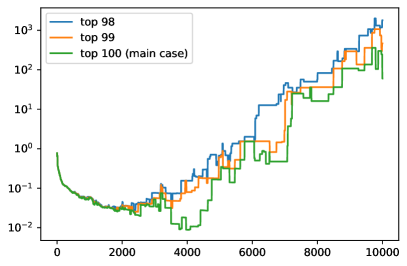
In our simulation studies we have 200 null hypotheses, all of them being , numbered from 1 to 200. The first 100 null hypotheses are false, and the true distribution is ; and the remaining 100 null hypotheses are true. At each step, from 1 to 10 000, we choose the hypothesis being tested randomly with equal probabilities, so that each hypothesis is chosen with probability . Figure 1 gives the plots for (meaning that we aim to discover all 100 false null hypotheses), , and . Let us call such plots discovery plots. We generate the 10 000 observations randomly with the standard seed of 42 for the random number generator (in fact, the results are very sensitive to the chosen value for the seed). The final value of the discovery plot for the top 100 martingale values () is approximately 60.1. Using Jeffreys’s [6, Appendix B] expression, there is very strong evidence that the top 100 martingale values exactly pinpoint the 100 false null hypotheses.
The martingale merging function used in Fig. 1 is . It is clear that any symmetric martingale merging function, which is a convex mixture of (Proposition 1 above), that does not have as its component, will produce very poor results for all discovery plots shown in Fig. 1: e.g., will be very small (approximately in our case), and , , will be even smaller.
While Fig. 1 uses the martingale merging function, using, e.g., would give similar results.
5 Almost family-wise multiple testing
Let us now relax the requirement (1) to
This requirement can be interpreted as almost all discoveries in being justified: we are allowing only one exception. The chronological discovery diagonal (2) now becomes the chronological discovery subdiagonal
The analogue of Algorithm 1 for the chronological discovery subdiagonal is given as Algorithm 2. In our simulation study we apply it to the martingale merging function . One complication is that it sometimes has to be applied to sequences of length 1, in which case we understand it to be the same as .
6 Dynamic confidence regions
Necessity measures discussed in Sect. 2 are only one possible way to package the idea of necessity. A much more standard way is to use confidence regions, which we will define in this section in our dynamic setting; our definitions will be natural modifications of the standard definitions (in the case of p-values) and the definitions given in [16, 15] (in the case of e-values). Let be a martingale test, fixed throughout this section.
We will be interested in confidence regions for the parameter , where is a mapping from the probability measures on the sample space to the parameter space (which can be any set). The exact confidence region for at time corresponding to the realized outcome and significance level is defined as
as usual, the dependence on is often suppressed. A confidence region is a set of parameter values containing the exact confidence region.
Alternatively, we can define a confidence region as a set such that
| (3) |
The exact confidence region is the smallest such set. In other words, satisfies (3), and any satisfying (3) contains , .
Finally, we can define the exact confidence region as the set of all satisfying .
One disadvantage of the dynamic notion of exact confidence regions is that, as a function of , is not decreasing: we are not guaranteed to have . This phenomenon of “losing evidence” and ways of partially preventing it are discussed in [4, 10] and [12, Chap. 11].
It is essential to have the martingale test fixed in advance in order to have valid confidence regions; on the other hand, confidence regions corresponding to different are valid simultaneously.
7 Multiple testing en masse
In this section we define, for each rejection set , a confidence region for the number of justified discoveries in (i.e., anomalous ). Such confidence regions are often of the form for some lower bound (we only have a lower confidence bound since can be arbitrarily close to being a test martingale without being one).
Given a rejection set , we are interested in the parameter
which is the number of justified discoveries. While in this paper we concentrate on the parameter function , this function can be generalized in various directions; see, e.g., [17, Remark 6.1].
The confidence region for at time at significance level consists of satisfying , where the possibility measure is
| (4) | ||||
Replacing by we also obtain a valid (perhaps conservative) confidence region. In the case of the optimal , we refer to
as the discovery matrix at time . It is a lower triangular matrix with and . In the case , the range of includes the empty set , and in this case we set to 1.
In the computational experiments reported in this paper, the discovery matrix is always monotonically decreasing in , and so
This is essential for the interpretation of our results. However, in general, the discovery matrix is not guaranteed to be decreasing in [17, 15], and so might need to be regularized by redefining ,
Algorithm 3 implements (4). In the case we have , and as discussed earlier, we set . This algorithm computes the discovery matrix in time when is a fixed or a fixed convex mixture of the first few ; this follows from being computable in time , which in turn follows from, e.g., Newton’s identities (see Appendix B). It is interesting that for the simulation studies reported in this paper we do not need more efficient algorithms such as the algorithm given in [15] and, in the case of , the algorithm given in [17]; computations take at most a couple of minutes on an ordinary laptop.


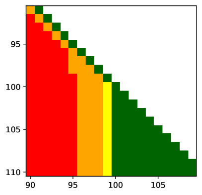
See Figs 3 and 4 for discovery matrices at time 10 000 for the same simulated data as before. The colour coding used in both figures involves much more extreme values of the possibility measures than the usual scheme used in [17, 15] (the scheme in [17, 15] uses the thresholds proposed by Jeffreys [6, Appendix B]):
-
•
The final martingale values below are shown in green. For such cells (in row and column ) we have , and these are exactly the cells for which we do not have strong evidence for there being at least justified discoveries.
-
•
The final martingale values between and are shown in yellow. These are exactly the cells for which we have strong but not decisive evidence for there being at least justified discoveries ().
-
•
The final martingale values between and are shown in orange. For these cells (and for the cells in the darker colours) we have decisive evidence for there being at least justified discoveries.
-
•
The final martingale values between and are shown in red.
-
•
The final martingale values between and are shown in dark red.
-
•
The final martingale values above are shown in black.
The diagonal of a discovery matrix consists of the cells , the justification for the offset of 1 being that in starts from 0 rather than 1. Correspondingly, the subdiagonal consists of , and the superdiagonal consists of .
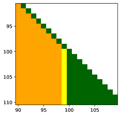
The diagonal, subdiagonal, and superdiagonal can be clearly seen in the right panels of the two figures. The diagonal can be traced starting from the top left corner of either bounding box. In both figures the diagonal (when moving south-east) is first orange, then yellow (just one cell), and then green. In Fig. 3 the subdiagonal is also first orange, then yellow (just one cell), and then green, but in Fig. 4 the subdiagonal is first red and only later becomes orange. The superdiagonal is green in both figures.
The corresponding confidence intervals (i.e., confidence regions that happen to be intervals) can be read off the two figures. For example, for each row , the non-green cells represent the confidence interval for the number of justified discoveries among the top martingale values at significance level 10. We can see that for the confidence interval is ; it is degenerate and contains only one value: we are predicting that all 100 null hypotheses with the largest final martingale values are justified (and a fortiori true) discoveries, and we have strong evidence for that. On the other hand, the green superdiagonal entry is very small (it is, approximately, ). If we raise the significance level to 100 (Jeffreys’s threshold for decisive evidence), the confidence interval widens to . And when we raise it further to the huge value of , the confidence interval (given by the non-red entries in the right panel) widens to .
Figures 3 and 4 suggest that discovery matrices are monotonically decreasing in the eastern and south-eastern directions and monotonically increasing in the southern direction. These properties of monotonicity (except for the monotonicity in discussed earlier) are stated and proved in [17] and [15].
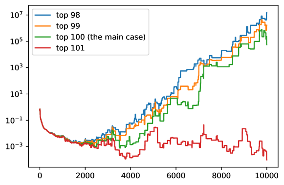
Figures 1 and 2 show the evolution of various entries of discovery matrices such as those in Figs 3 and 4 over time. The green lines in both panels of Fig. 1 show the evolution of the diagonal entry over the 10 000 observations. The orange and blue lines in Fig. 1 show the evolution of the entries and , respectively. All these entries lie on the diagonal
of the discovery matrix at time 10 000. We talked about family-wise validity in Sect. 4 since is the largest significance level at which the confidence interval is a one-element set, namely .
The right panel of Fig. 1 also shows, as red line, the evolution of the diagonal entry . This line shows that the green entry in Fig. 3 is very small; in numbers, the final value of the red line in Fig. 1 (i.e., in Fig. 3) is, approximately, ). The value of in Fig. 4 is even smaller.
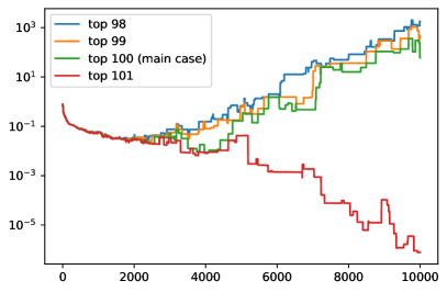
The green line in Fig. 2 shows the evolution of the entry , which determines the significance levels at which the confidence interval for the number of justified discoveries is (allowing one unjustified discovery). Its final value corresponds to the entry in Fig. 4, and the two numbers have the same order of magnitude (they are, however, different because Figs 2 and 4 use different martingale merging functions, vs ). The orange and blue lines in Fig. 2 are interpreted in the same way; they correspond to the entries and , respectively, of Fig. 4. The red line in Fig. 2, however, disagrees sharply with the entry of Fig. 4, because the martingale merging function used in Fig. 4 has as its component.
8 Conclusion
These are some possible directions of further research:
-
•
The motivation behind this paper is coming from game-theoretic probability and statistics, but its mathematical setting is that of measure-theoretic probability. Replacing measure-theoretic probability by purely game-theoretic probability (as developed in [12]) would simplify the exposition and lead to more natural and general definitions.
-
•
This paper concentrates on simulation studies. It would be interesting to conduct empirical studies on benchmark or real-world datasets, for example ones collected in the course of statistical meta-analyses.
-
•
The experimental results of Sect. 7 establish confidence regions for the numbers of true discoveries, which can be restated as results about the false discovery proportions, FDP. Are there any interesting theoretical results in this context about false discovery rates, FDR (as in [1] in the case of p-values and [19] in the case of e-values)?
-
•
This paper concentrates on the closed setting (when the number of null hypotheses is given in advance). The open setting, where new hypotheses may appear at any moment, may be even more interesting. In this case we need, of course, to break the symmetry between the null hypotheses: there is no uniform probability measure on .
Acknowledgments
Many thanks to Jean Gallier for his advice on literature and for correcting the statement of Lemma 4.1.3 in [5]. My research has been partially supported by Mitie.
References
- [1] Yoav Benjamini and Yosef Hochberg. Controlling the false discovery rate: a practical and powerful approach to multiple testing. Journal of the Royal Statistical Society B, 57:289–300, 1995.
- [2] Nicolas Bourbaki. Elements of Mathematics. Algebra II. Chapters 4–7. Springer, Berlin, 2003.
- [3] Henri Cartan. Calcul différentiel. Hermann, Paris, 1967.
- [4] A. Philip Dawid, Steven de Rooij, Glenn Shafer, Alexander Shen, Nikolai Vereshchagin, and Vladimir Vovk. Insuring against loss of evidence in game-theoretic probability. Statistics and Probability Letters, 81:157–162, 2011.
- [5] Jean Gallier. Curves and Surfaces in Geometric Modeling: Theory and Algorithms. Morgan Kaufmann, San Francisco, CA, 2000. An updated version (2024) is available from the author’s website (accessed in March 2024).
- [6] Harold Jeffreys. Theory of Probability. Oxford University Press, Oxford, third edition, 1961.
- [7] W. Keith Nicholson. Introduction to Abstract Algebra. Wiley, New York, second edition, 1999. Fourth edition: 2012.
- [8] Glenn Shafer. The Art of Causal Conjecture. MIT Press, Cambridge, MA, 1996.
- [9] Glenn Shafer. A counterexample to Richard von Mises’s theory of collectives, by Jean Ville. Available on the web (accessed in March 2024), 2005.
- [10] Glenn Shafer, Alexander Shen, Nikolai Vereshchagin, and Vladimir Vovk. Test martingales, Bayes factors, and p-values. Statistical Science, 26:84–101, 2011.
- [11] Glenn Shafer and Vladimir Vovk. Probability and Finance: It’s Only a Game! Wiley, New York, 2001.
- [12] Glenn Shafer and Vladimir Vovk. Game-Theoretic Foundations for Probability and Finance. Wiley, Hoboken, NJ, 2019.
- [13] Jean Ville. Etude critique de la notion de collectif. Gauthier-Villars, Paris, 1939.
- [14] Richard von Mises. Grundlagen der Wahrscheinlichkeitsrechnung. Mathematische Zeitschrift, 5:52–99, 1919.
- [15] Vladimir Vovk and Ruodu Wang. True and false discoveries with independent e-values. Technical Report arXiv:2003.00593 [stat.ME], arXiv.org e-Print archive, March 2020.
- [16] Vladimir Vovk and Ruodu Wang. E-values: Calibration, combination, and applications. Annals of Statistics, 49:1736–1754, 2021.
- [17] Vladimir Vovk and Ruodu Wang. Confidence and discoveries with e-values. Statistical Science, 38:329–354, 2023. Revised arXiv version: arXiv:1912.13292 [math.ST] (November 2022).
- [18] Vladimir Vovk and Ruodu Wang. Merging sequential e-values via martingales. Electronic Journal of Statistics, 18:1185–1205, 2024.
- [19] Ruodu Wang and Aaditya Ramdas. False discovery rate control with e-values. Journal of the Royal Statistical Society B, 84:822–852, 2022.
Appendix A Proofs
In this appendix I will prove Propositions 1 and 2 (and state and prove a new Proposition 4). A multiaffine function is a multivariate function that is affine in each of its arguments. (So that multiaffine polynomials are multiaffine functions, and in Sect. A.1 we will see that these two notions are equivalent.) The proofs will follow from the following lemma.
Lemma 3.
A martingale merging function must be multiaffine.
Proof.
Let be a martingale merging function. We are required to prove
| (5) |
where . Let us fix , and . Consider the sample space with the natural filtration and a positive probability measure (i.e., for any ). Suppose that the set of sample points where
for some uncorrelated test martingales is non-empty, and let be such a sample point. Suppose that in our probability space we have the branching probability
and that the martingale satisfies
The existence of such a probability space and uncorrelated test martingales is obvious. Since
is a test martingale, we have
which is equivalent to (5). ∎
A.1 Proof of Proposition 1
To show that a martingale merging function is a multiaffine polynomial, we combine Lemma 3 with Lemma 4.1.3 in [5] (whose proof relies on Cartan’s method of successive differences [3, Sect. 6.3]). According to [5, Lemma 4.1.3], a multiaffine function of arguments has the form
where are multilinear functions (i.e., functions linear in each argument). It remains to notice that
for some constant ; indeed,
Let us now check that a martingale merging function is a positive multiaffine polynomial. Suppose there is a negative coefficient in front of one or more of its monomials. Choose and fix a monomial with a negative coefficient. Set all variables that do not occur in this monomial to zero. Set each of the variables that do occur in this monomial to and let . For a large enough , the value of the polynomial (the value being a univariate polynomial in with a negative leading coefficient) will become negative, which is impossible.
There is a minor gap in our derivation of Proposition 1 from [5, Lemma 4.1.3]: the latter assumes that the multiaffine function is defined on an affine space whereas in our context is defined on . Let us check that every affine can be extended to an affine . We proceed by induction and show that if is an affine function with ranging over we can extend it to an affine function with ranging over (with the ranges of the other arguments of unchanged). Without loss of generality, let . We extend to by the affinity in : for any ,
| (6) |
We only need to check that is multiaffine. The affinity in holds by construction, so we only need to check that is affine in for . Without loss of generality, let . Since the arguments of and are kept fixed, we will ignore them. Our goal is to show that
| (7) |
for . By the definition (6), the equality (7) is equivalent to
| (8) |
It remains to notice that (8) can be derived as linear combination of
| (9) |
and
| (10) |
A.2 Proof of Proposition 2
A.3 Comparisons with merging independent and sequential e-values
In this subsection we will discuss ie-merging and se-merging functions, to be defined momentarily; for a further discussion of these functions see, e.g., [18].

Suppose are admissible independent e-variables (i.e., nonnegative random variables that are independent and satisfy , ) or admissible sequential e-variables (i.e., nonnegative, adapted, and satisfying , ). Then
are uncorrelated test martingales with final values . Therefore, any normalized positive multiaffine polynomial (NPMAP) is an ie-merging function, in the sense of mapping any (admissible) independent e-variables to an e-variable (i.e., nonnegative random variable satisfying ); moreover, any NPMAP is an se-merging function, in the sense of mapping any (admissible) sequential e-variables to an e-variable. This gives us the structure shown in Fig. 5: it is obvious that every se-merging function is an ie-merging function.
Let us check that both inclusions in the Euler diagram shown in Fig. 5 are strict. The outer inclusion is strict since the function
| (11) |
is an admissible ie-merging function [16, Remark 4.3] while it is not an se-merging function [18, Example 2]. To see that the inner inclusion is strict, notice that
is an se-merging function for any function taking values in , even highly non-linear one, such as .

Specializing Fig. 5 to symmetric merging functions we obtain Fig. 6. The function (11) is symmetric and so can also serve as an example demonstrating that the outer inclusion in Fig. 6 is strict. On the other hand, the following proposition shows that the inner inclusion in Fig. 6 is strict in an uninteresting way.
Proposition 4.
Every symmetric se-merging function is dominated by a convex mixture of NESPs.
Proof.
Theorem 1 in [18] says that any se-merging function is dominated by a martingale merging function (where “martingale merging function” is used in a sense different from this paper; this proof uses “martingale merging function” in the sense of [18]). By definition, a martingale merging function is affine in its last argument. By symmetry, it is affine in each argument. It remains to follow the reasoning of Sects A.1 and A.2. ∎
Appendix B Computing NESPs
In this appendix we will discuss how to compute the NESP for a fixed efficiently, namely, in time . We will use the fact that the polynomials can be computed in time , and so one way to compute efficiently is to express them via .
These are the efficient representations for the first few NESPs:
It is clear that such a representation exists for any fixed , and it allows us to compute in time . In terms of Bell polynomials
where is the set of natural numbers, the general expression is
where .