claimClaim remarkRemark hypothesisHypothesis

An algorithm for the Riemannian logarithm on StiefelSimon Mataigne, Ralf Zimmermann, Nina Miolane






An efficient algorithm for the Riemannian logarithm on the Stiefel manifold for a family of Riemannian metrics


Simon Mataigne
UCLouvain, ICTEAM, Louvain-la-Neuve, Belgium. Simon Mataigne is a Research Fellow of the Fonds de la Recherche Scientifique - FNRS. 
simon.mataigne@uclouvain.be

  
Ralf Zimmermann
University of Southern Denmark, Department of Mathematics and Computer Science,
Odense, Denmark.

zimmermann@imada.sdu.dk

  
Nina Miolane
UC Santa Barbara, Electrical and Computer Engineering, Santa Barbara, CA. 
ninamiolane@ucsb.edu




Abstract
Since the popularization of the Stiefel manifold for numerical applications in 1998 in a seminal paper from Edelman et al., it has been exhibited to be a key to solve many problems from optimization, statistics and machine learning. In 2021, Hüper et al. proposed a one-parameter family of Riemannian metrics on the Stiefel manifold, subsuming the well-known Euclidean and canonical metrics. Since then, several methods have been proposed to obtain a candidate for the Riemannian logarithm given any metric from the family. Most of these methods are based on the shooting method or rely on optimization approaches. For the canonical metric, Zimmermann proposed in 2017 a particularly efficient method based on a pure matrix-algebraic approach. In this paper, we derive a generalization of this algorithm
that works for the one-parameter family of Riemannian metrics. The algorithm is proposed in two versions, termed backward and forward, for which we prove that it conserves the local linear convergence previously exhibited in Zimmermann’s algorithm for the canonical metric.


keywords: 
Stiefel manifold, Riemannian logarithm, geodesic distance, Riemannian metric




15B10, 15B57, 53Z50, 65B99, 15A16




1 Introduction


The field of statistics on manifolds has experienced significant growth in recent years, driven by a multitude of applications involving manifold-valued data — such as orthogonal frames, subspaces, fixed-rank matrices, diffusion tensors or shapes — that need to undergo processes like denoising, resampling, extrapolation, compression, clustering, or classification (see, e.g., [8, 19, 20, 27]). Given a Riemannian manifold $\mathcal{M}$, both statistical and numerical applications often require the computation of distances between data points $U$ and $\widetilde{U}\in\mathcal{M}$ [14]. Calculating this distance relies on an oracle that provides a minimal geodesic between the two points. A minimal geodesic is a curve whose length corresponds to the Riemannian distance between $U$ and $\widetilde{U}$. Most geometries lack a known closed-form expression for the minimal geodesic between any two points. Consequently, algorithms must be developed for these geometries to yield a candidate for the minimal geodesic. The Stiefel manifold falls into this category. It has gained popularity since the publication of the seminal paper [13] by Edelman et al.. This manifold finds applications in various fields, including statistics [11], optimization [13], and deep learning [15, 17].
The implementation of the Stiefel manifold is notably available in software packages such as Geomstats [21], Manopt [7], Manopt.jl [4].


It has been demonstrated in [35] that the Stiefel manifold, equipped with any Riemannian metric from the one-parameter family introduced in [18], features at least one minimal geodesic between any two points. However, computing any geodesic between two given points on the Stiefel manifold is a challenging task, known as the geodesic endpoint problem. Several research efforts have proposed numerical methods to address this issue [25, 28, 31, 34, 35]. Unfortunately, none of these methods guarantees the computation of a minimal geodesic, referred to as the logarithm problem.


The one-parameter family of metrics introduced in [18] includes the well-known Euclidean and canonical metrics [13].
In [24], it was observed that this family of metrics can be considered as metrics arising from a Cheeger deformation. Cheeger deformation metrics were first introduced in [12] and have since been used in Riemannian geometry to construct metrics with special features, e.g., non-negative curvature, or Einstein metrics. We refer to [24] for further details and additional references.
Numerical algorithms for computing geodesics and Riemannian normal coordinates under this family of metrics were introduced in [35] and [25].
The case of the canonical metric allowed for special treatment, which was exploited in [35, Algorithm 4] and earlier in [34]. The associated algorithm has proven local linear convergence. In the comparative study of [35], it turned to be the most efficient and robust numerical approach. It was therefore a shortcoming that [35, Algorithm 4] was only designed to work with the canonical metric.


Original contribution


In this paper, we generalize [35, Algorithm 4] to the family of metrics introduced in [18]. The algorithm is provided in two versions, termed backward and forward. For the backward iteration, we show the local linear convergence of the algorithm and we obtain an explicit expression for the convergence rate, generalizing the one obtained in [35, Proposition 7]. However, performing a backward iteration requires to solve a costly sub-problem (although simpler than the main problem). To alleviate the computational costs, we introduce three types of forward iterations. These iterations are much cheaper than the backward iteration while preserving the local linear convergence of the algorithm.



Reproducibility statement


All the codes written to produce results and figures are available at the address https://github.com/smataigne/StiefelLog.jl.



Organization


The paper is structured as follows. We start by recalling the necessary background on the Stiefel manifold in Section 2. In Section 3, we recap
[35, Algorithm 4] and its convergence result. We generalize the approach to the family of metrics in Section 4, where we provide a convergence analysis for the backward and forward iterations. Then, we compare the performance of the new algorithms with each other in Section 5. Finally, the convergence radius and the benchmark with methods from the state of the art is carried out in Section 6.



Notations


For $p>0$, we denote the $p\times p$ identity matrix by ${I}_{p}$. For $n>p>0$, we define




$${I}_{n\times p}:=\begin{bmatrix}{I}_{p}\\
{0}_{n-p\times p}\end{bmatrix}\text{ and }{I}_{p\times n}:={I}_{n\times p}^{T}.$$



$\mathrm{Skew}(p)$ is the set of $p\times p$ skew-symmetric matrices (${A}=-{A}^{T})$ and the orthogonal group of $p\times p$ matrices is written as




$$\mathrm{O}(p):=\{{Q}\in\mathbb{R}^{p\times p}\ |\ {Q}^{T}{Q}={I}_{p}\}.$$



The special orthogonal group $\mathrm{SO}(p)$ is the subset of matrices of $\mathrm{O}(p)$ with positive unit determinant. An orthogonal completion ${U}_{\perp}$ of ${U}\in\mathbb{R}^{n\times p}$ is ${U}_{\perp}\in\mathbb{R}^{n\times n-p}$ such that $\begin{bmatrix}{U}&{U}_{\perp}\end{bmatrix}\in\mathrm{O}(n)$. Throughout this paper, $\exp$ and $\log$ always denote the matrix exponential and the principal matrix logarithm. The Riemannian exponential and logarithmic maps are written with capitals, Exp and Log. Finally, $\|\cdot\|_{2}$ denotes the spectral matrix norm.



2 Background on the Stiefel manifold


The main references for this section are [1, 13, 35]. Given integers $n>p>0$, the Stiefel manifold of orthonormal $p$-frames in $\mathbb{R}^{n}$ is defined as



(1)

$$\mathrm{St}(n,p):=\{{U}\in\mathbb{R}^{n\times p}\ |\ {U}^{T}{U}={I}_{p},\ n>p\}.$$



If $n=p$, the Stiefel manifold reduces to the orthogonal group, $\mathrm{St}(n,n)=\mathrm{O}(n)$. This case allows for special treatment and is extensively studied. In particular, the minimal geodesics are known in closed form. Therefore, we restrict our considerations to $n>p$. The Stiefel manifold is a differentiable manifold of dimension $np-\frac{p(p+1)}{2}$ [1]. The tangent space of $\mathrm{St}(n,p)$ at a point ${U}$ can be written as




$$T_{U}\mathrm{St}(n,p)
=\{{\Delta}\in\mathbb{R}^{n\times p}\ |\ {U}^{T}{\Delta}+{\Delta}^{T}{U}={0}\}.$$




It follows that for all ${\Delta}\in T_{U}\mathrm{St}(n,p)$, we can write ${\Delta}={UA}+{U}_{\perp}{B}$ where ${A}\in\mathrm{Skew}(p)$, ${B}\in\mathbb{R}^{(n-p)\times p}$ and ${U}_{\perp}\in\mathrm{St}(n,n-p)$ is an orthogonal complement of ${U}$. The concept of tangent space is illustrated on Figure 1. Notice that for a given ${\Delta}\in T_{U}\mathrm{St}(n,p)$, ${A}$ is uniquely defined while ${B}$ depends on the chosen completion ${U}_{\perp}$. Indeed ${U}_{\perp}{B}=({U}_{\perp}{R})({R}^{T}{B})$ for all ${R}\in\mathrm{O}(p)$.
(For the initiated reader, we mention that selecting a specific completion ${U}_{\perp}$ corresponds to lifting the tangent vector $\Delta$ to a specific horizontal space. We omit the details.)



2.1 Metrics and distances


Let $\mathcal{M}$ be a differentiable manifold. A Riemannian metric on $\mathcal{M}$ is a family $\{\langle\cdot,\cdot\rangle^{p}:\mathrm{T}_{p}\mathcal{M}\times\mathrm{T}_{p}\mathcal{M}\mapsto\mathbb{R}\}_{p\in\mathcal{M}}$ of symmetric positive definite bi-linear forms that depends smoothly on the location $p$.
In practice, the input arguments of the metric encode its dependency on $p$, so that we can write $\langle\cdot,\cdot\rangle$ without ambiguity. Edelman et al. [13] introduced two natural metrics on the Stiefel manifold, called the Euclidean and the canonical metric, respectively. These two metrics are subsumed by the family of metrics introduced in [18]. For convenience, we use another parameterization of this family and define the $\beta$-metric with $\beta>0$ as follows. For all ${\Delta},\widetilde{{\Delta}}\in\mathrm{T}_{U}\mathrm{St}(n,p)$,




$$\langle{\Delta},\widetilde{{\Delta}}\rangle_{\beta}=\operatorname{\mathrm{Tr}}{\Delta}^{T}({I}_{n}-(1-\beta){UU}^{T})\widetilde{{\Delta}}=\beta\operatorname{\mathrm{Tr}}{A}^{T}\widetilde{{A}}+\operatorname{\mathrm{Tr}}{B}^{T}\widetilde{{B}}.$$



The Euclidean and canonical metrics correspond to $\beta=1$ and $\beta=\frac{1}{2}$ respectively. Therefore, we are particularly interested in $\beta\in\left[\frac{1}{2},1\right]$ and our experiments will focus on this interval. The Euclidean metric is inherited from the ambient Euclidean space $\mathbb{R}^{n\times p}$ while the canonical metric is inherited from the quotient structure $\mathrm{St}(n,p)=\mathrm{SO}(n)/\mathrm{SO}(n-p)$ [13]. The norm induced by any $\beta$-metric is $\|{\Delta}\|_{\beta}=\sqrt{\langle{\Delta},{\Delta}\rangle_{\beta}}$, and the length of a continuously differentiable curve $\gamma:[0,1]\mapsto\mathrm{St}(n,p)$ is given by



(2)

$$l_{\beta}(\gamma)=\int_{0}^{1}\|\dot{\gamma}(t)\|_{\beta}\ \mathrm{d}t,$$



where $\dot{\gamma}$ denotes the time derivative of $\gamma$. For all ${U},\widetilde{{U}}\in\mathrm{St}(n,p)$, we obtain an induced distance function [29, Proposition 1.1] (also termed Riemannian distance) defined as



(3)

$$d_{\beta}({U},\widetilde{{U}})=\inf\{l_{\beta}(\gamma)\ |\ \gamma(0)={U},\ \gamma(1)=\widetilde{{U}}\}.$$



Since $\beta$-geodesics exist for all times [18], the Hopf-Rinow theorem ensures that a curve achieves the minimal distance: the “$\inf$” in (3) is a “$\min$” on $\mathrm{St}(n,p)$.


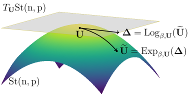
Figure 1: Conceptual illustration of the Stiefel manifold $\mathrm{St}(n,p)$, the tangent space $T_{U}\mathrm{St}(n,p)$, the exponential map $\mathrm{Exp}_{\beta,{U}}({\Delta})$ and the logarithmic map $\mathrm{Log}_{\beta,{U}}(\widetilde{U})$ (see Section 2.2).


Riemannian metrics act on tangent vectors, the Riemannian distance is for points on the manifold. Since $\mathrm{St}(n,p)$ is embedded in $\mathbb{R}^{n\times p}$, the distance between $U,\tilde{U}\in\mathrm{St}(n,p)$ can also be measured in the ambient space. An upper bound for this distance in the Frobenius norm is




$$\|U-\tilde{U}\|_{F}\leq\|U\|_{F}+\|\tilde{U}\|_{F}=2\sqrt{\text{trace}(I_{p})}=2\sqrt{p},$$



and is refererred to as the Frobenius diameter of the Stiefel manifold.




2.2 The exponential and logarithm maps


Consider $\mathrm{St}(n,p)$ endowed with $\langle\cdot,\cdot\rangle_{\beta}$, written $\left(\mathrm{St}(n,p),\langle\cdot,\cdot\rangle_{\beta}\right)$. Zimmermann and Hüper [35] showed that the exponential map $\mathrm{Exp}_{\beta,{U}}:T_{U}\mathrm{St}(n,p)\mapsto\mathrm{St}(n,p)$, i.e., the function that maps ${\Delta}\in T_{U}\mathrm{St}(n,p)$ to the point reached at unit time by the geodesic with starting point ${U}$ and initial velocity ${\Delta}$ (see, e.g., [29, Chap. II, Sec. 2]), can be expressed according to Theorem 2.1. The mode of operation of the exponential map is illustrated in Figure 1.



Theorem 2.1.


The exponential map [35, Equation 10].
For all ${U}\in\mathrm{St}(n,p)$ and ${\Delta}\in T_{U}\mathrm{St}(n,p)$,



(4)

$$\mathrm{Exp}_{\beta,{U}}({\Delta})=\begin{bmatrix}{U}&\ {Q}\end{bmatrix}\exp\left(\begin{bmatrix}2\beta{A}&-{B}^{T}\\
{B}&{0}\end{bmatrix}\right){I}_{n\times p}\exp\left((1-2\beta){A}\right),$$



where ${A}={U}^{T}{\Delta}\in\mathrm{Skew}(p)$ and ${Q}{B}=({I}-{U}{U}^{T}){\Delta}\in\mathbb{R}^{n\times p}$ is any matrix decomposition where ${Q}\in\mathrm{St}(n,n-p)$ with ${Q}^{T}{U}={0}$ and ${B}\in\mathbb{R}^{n-p\times p}$.




If $n>2p$, we can always reduce the decomposition of ${\Delta}$ such that ${Q}\in\mathrm{St}(n,p)$ and ${B}\in\mathbb{R}^{p\times p}$ [28, 35].
The first matrix exponential of (4) belongs then to $\mathbb{R}^{2p\times 2p}$ instead of $\mathbb{R}^{n\times n}$. Given $U,\widetilde{U}\in\mathrm{St}(n,p)$, the logarithmic map $\mathrm{Log}_{\beta,{U}}(\widetilde{{U}})$ is the function that returns the set of all minimal-norm tangent vectors $\Delta\in T_{U}\mathrm{St}(n,p)$ such that $\mathrm{Exp}_{\beta,{U}}({\Delta})=\widetilde{U}$. Locally, the logarithmic map is the inverse of the exponential map.



Problem 2.2.


The Logarithm problem.
Let ${U},{\widetilde{U}}\in\mathrm{St}(n,p)$ and $\beta>0$. The logarithmic map $\mathrm{Log}_{\beta,{U}}(\widetilde{{U}})$ returns all ${\Delta}\in T_{{U}}\mathrm{St}(n,p)$ such that




$$\mathrm{Exp}_{\beta,{U}}({\Delta})=\widetilde{{U}}\text{ and }\|{\Delta}\|_{\beta}=d_{\beta}({U},\widetilde{{U}}).$$



The curves $[0,1]\ni t\mapsto\mathrm{Exp}_{\beta,{U}}(t{\Delta})$ are then minimal geodesics.




Because the Stiefel manifold is complete, the Hopf-Rinow theorem [10, Chap. 7, Thm. 2.8] ensures the existence of a minimal geodesic between any two points on the Stiefel manifold. However, on compact Riemannian manifolds, every geodesic has a designated cut time $t^{*}$ [29]: the geodesic stays minimal as long as $t\leq t^{*}$, not beyond. The point $\mathrm{Exp}_{\beta,{U}}(t^{*}{\Delta})$ is termed the cut point. Consequently, when a geodesic between two points is established, the shooting direction is a logarithm if and only if the destination is reached before the cut point.
In [35, Thm. 3], it is emphasized that the logarithm problem on the Stiefel manifold boils down to solving a nonlinear matrix problem. Very recent works [2, 30] proposed a thin interval for the injectivity radius $\mathrm{inj}_{\mathrm{St}(n,p)}$, i.e., the distance to the nearest cut point. In particular for $\beta=\frac{1}{2}$, they showed that $0.894\pi<\mathrm{inj}_{\mathrm{St}(n,p)}<0.914\pi$. Within the injectivity radius, any solution to the geodesic endpoint problem gives the unique solution to Problem 2.2



3 State of the art


[28, 34] introduced an efficient method to obtain a geodesic between any two given points ${U},{\widetilde{U}}\in\mathrm{St}(n,p)$, but only in the case of the canonical metric ($\beta=\frac{1}{2}$) and $n\geq 2p$. The algorithm was enhanced in [35] to obtain a better convergence rate. Its pseudo-code is given by Algorithm 1. Previous experiments [35, Table 1] highlighted the better performance of Algorithm 1 compared to the shooting method, introduced first in [9]. For the $\beta$-metric, [25] also proposed a L-BFGS method inspired from the shooting method. The L-BFGS method was however shown to converge slower than the shooting method [25, Table 2]. This observation provides a strong incentive to generalize Algorithm 1 to the parameterized family of $\beta$-metrics.


Algorithm 1 finds a $\Delta$ satisfying $\widetilde{U}=\mathrm{Exp}_{\beta,U}(\Delta)$ when $\beta=\frac{1}{2}$. In this case, Problem 2.2 simplifies and consists of finding ${A}\in\mathrm{Skew}(p),{B}\in\mathbb{R}^{p\times p}$ such that



(5)

$$\begin{bmatrix}{M}\\
{N}\end{bmatrix}=\exp\begin{bmatrix}{A}&-{B}^{T}\\
{B}&{0}\end{bmatrix}{I}_{2p\times p},$$



where ${M}:={U}^{T}\widetilde{U}$, ${N}:={Q}^{T}\widetilde{U}$ with ${Q}\in\mathrm{St}(n,p)$ and ${Q}^{T}{U}={0}$. It is solved iteratively by computing a sequence $\{{A}_{k},{B}_{k},{C}_{k}\}_{k\in\mathbb{N}}$ by



(6)

$$\begin{bmatrix}{A}_{k}&-{B}_{k}^{T}\\
{B}_{k}&{C}_{k}\end{bmatrix}:=\log{V}_{k}\in\mathrm{Skew}(2p)\text{ with }{V}_{k}:=\begin{bmatrix}{M}&{O}_{k}\\
{N}&{P}_{k}\end{bmatrix}\in\mathrm{SO}(2p).$$



$O_{0},P_{0}$ are chosen such that $V_{0}\in\mathrm{SO}(2p)$ and ${V}_{k}$ is updated to have $\lim_{k\rightarrow\infty}\|{C}_{k}\|_{2}=0$. Theorem 3.2 below shows that taking ${V}_{k+1}={V}_{k}\begin{bmatrix}{I}_{p}&{0}\\
{0}&\exp({\Gamma}_{k})\end{bmatrix}$, where ${\Gamma}_{k}$ solves the Sylvester equation



(7)

$${S\Gamma}_{k}+{\Gamma}_{k}{S}={C}_{k}\text{ with }{S}:=\frac{1}{12}{B}_{k}{B}_{k}^{T}-\frac{{I}_{p}}{2},$$



yields local linear convergence, i.e., $\|{C}_{k+1}\|_{2}\leq a\|{C}_{k}\|_{2}+\mathcal{O}(\|{C}_{k}\|_{2}^{2})$ with $a<1$ (see Theorem 3.2). Ultimately, Algorithm 1 outputs a geodesic $\gamma:[0,1]\mapsto\operatorname{\mathrm{St}}(n,p)$ between ${U}$ and $\widetilde{U}$ defined by



(8)

$$\gamma(t):=\mathrm{Exp}_{\frac{1}{2},{U}}(t{\Delta})=\begin{bmatrix}{U}&{Q}\end{bmatrix}\exp\left(t\begin{bmatrix}{A}_{\infty}&-{B}^{T}_{\infty}\\
{B}_{\infty}&{0}\end{bmatrix}\right){I}_{2p\times p}.$$



Algorithm 1 possesses two strengths. First, $\{{A}_{k},{B}_{k},{C}_{k}\}$ provides a curve between ${U}$ and $\widetilde{U}$ at any iteration $k$, which becomes a (numerical) geodesic at convergence when $\|{C}_{k}\|_{2}<\epsilon$. Second, unlike the shooting method, no time-discretization of the geodesic is needed. This is a strong advantage since i) the discretization is computationally expensive: an exponential map and an approximate parallel transport have to be computed at every discretized point along the geodesic and ii) the level of discretization is a user-parameter that has to be tuned, or guessed.
On the other hand, the shooting method involves computing the matrix exponential of skew-symmetric matrices. At this day, it can be done more efficiently — such as in SkewLinearAlgebra.jl — than computing the matrix logarithm in (6). Nonetheless [35, Table 1] observed that Algorithm 1 runs faster due to its better convergence rate. It was thus a deficiency that the most efficient method among the considered ones could not be generalized to the $\beta$-metrics. We close this gap in the next sections.


Algorithm 1  [35, Algorithm 4] Improved algebraic Stiefel logarithm for the canonical metric ($\beta=\frac{1}{2}$).


1:  INPUT: Given ${U},\widetilde{U}\in\operatorname{\mathrm{St}}(n,p)$, $n\geq 2p$ and $\epsilon>0$, compute:



2:  ${M}={U}^{T}\widetilde{U}$



3:  $\widehat{Q}\widehat{N}=({I}-{U}{U}^{T})\widetilde{U}$                                    #where $\widehat{Q}\in\mathrm{St}(n,p)$ and $\widehat{Q}^{T}U=0$.



4:  ${V}_{0}=\begin{bmatrix}{M}&{O}_{0}\\
{N}&{P}_{0}\end{bmatrix}\in\mathrm{SO}(2p),\ Q\in\mathrm{St}(n,p)$   #see Appendix B to choose ${N,O_{0},P_{0},Q}$.



5:  for $k=0,1,...$ do





6:     $\begin{bmatrix}{A}_{k}&-{B}_{k}^{T}\\
{B}_{k}&{C}_{k}\end{bmatrix}=\log{V}_{k}$



7:     if $\|{C}_{k}\|\leq\epsilon$ then





8:        break



9:     end if


10:     Compute ${\Gamma}_{k}$ solving ${\Gamma}_{k}{S}+{S\Gamma}_{k}={C}_{k}$ where ${S}:=\frac{1}{12}{B}_{k}{B}_{k}^{T}-\frac{{I}_{p}}{2}$.



11:     ${V}_{k+1}={V}_{k}\begin{bmatrix}{I}_{p}&0\\
0&\exp({\Gamma}_{k})\end{bmatrix}$



12:  end for



13:  return  ${\Delta}={U}{A}+{QB}\in\operatorname{T_{U}\mathrm{St}(n,p)}$






Remark 3.1.


In line 3 of Algorithm 1, [34] proposed to compute a thin QR decomposition ${QN}=({I}-{U}{U}^{T})\widetilde{U}$. It is without ambiguity if $({I}-{U}{U}^{T})\widetilde{U}$ has full column rank. However, if $({I}-{U}{U}^{T})\widetilde{U}$ is not full column rank, it is important to ensure ${Q}\in\mathrm{St}(n,p)$ with ${Q}^{T}{U}={0}$. Otherwise, Algorithm 1 may fail to find any ${\Delta}\in\mathrm{Log}_{\beta,U}(\widetilde{U})$.
Indeed, there are provable cases where



(9)

$$\mathrm{rank}(({I}-{U}{U}^{T})\Delta)>\mathrm{rank}(({I}-{U}{U}^{T})\widetilde{U}).$$



We show in Appendix A that (9) can only happen if $\widetilde{U}$ belongs to the cut locus of $U$.




The linear convergence result for Algorithm 1 is given by Theorem 3.2. In Section 4.3,
we first generalize the algorithm to work with the parametric family of metrics in form of Algorithm 2.
The associated generalization of the convergence statement Theorem 3.2 is then Theorem 4.3, which reduces to the original result for $\beta=\frac{1}{2}$.



Theorem 3.2.


[35, Prop. 7]
Given ${U},\widetilde{U}\in\mathrm{St}(n,p)$ $({U}\neq\widetilde{U})$ such that Algorithm 1 converges. Assume further that there is $0<\delta<1$ such that for $\log({V}_{k})=\begin{bmatrix}{A}_{k}&-{B}_{k}^{T}\\
{B}_{k}&{C}_{k}\end{bmatrix}$, it holds $\|\log({V}_{k})\|_{2}<\delta$ throughout the algorithm’s iteration loop. Then, for $k$ large enough, it holds



(10)

$$\|{C}_{k+1}\|_{2}\leq\frac{6}{6-\delta^{2}}\frac{\delta^{4}}{1-\delta}\|{C}_{k}\|_{2}+\mathcal{O}(\|{C}_{k}\|_{2}^{2}).$$







Theorem 3.2 highlights that the closer ${U}$ and $\widetilde{U}$, the faster Algorithm 1 should converge. This property was numerically confirmed in [34, Sec. 5.3].



4 The generalization of Algorithm 1



We propose a new approach to generalize Algorithm 1 to all the $\beta$-metrics. Still, we assume $n\geq 2p$ which matches the ‘$n\gg p$’ setting of practical big-data applications.


When $\beta\neq\frac{1}{2}$, a generalization of Algorithm 1 consists of finding
a sequence $\{{A}_{k},{B}_{k},{C}_{k}\}_{k\in\mathbb{N}}$ with ${A}_{k},C_{k}\in\mathrm{Skew}(p),{B}_{k}\in\mathbb{R}^{p\times p}$ such that



(11)

$$\begin{bmatrix}{M}\\
{N}\end{bmatrix}=\exp\begin{bmatrix}2\beta{A}_{k}&-{B}_{k}^{T}\\
{B}_{k}&{C}_{k}\end{bmatrix}{I}_{2p\times p}\exp((1-2\beta){A}_{k}),$$



where ${M}:={U}^{T}\widetilde{U}$, ${N}:={Q}^{T}\widetilde{U}$ (${Q}\in\mathrm{St}(n,p)$, ${Q}^{T}{U}={0}$)
and $\lim_{k\rightarrow\infty}\|{C}_{k}\|_{2}=0$. Since $A_{k}$ appears twice in (11), it is a challenging non-linear equation to solve. Moreover, straightforward usage of Newton’s method is very expensive [35]. However, the equation can be tackled by constructing a sequence



(12)

$$\begin{bmatrix}2\beta{A}_{k}&-{B}_{k}^{T}\\
{B}_{k}&{C}_{k}\end{bmatrix}:=\log\left({V}_{k}\begin{bmatrix}\exp(-(1-2\beta)\widehat{{A}}_{k})&0\\
0&{I}_{p}\end{bmatrix}\right),$$



where $\widehat{{A}}_{k}$ is a consistent approximation, i.e., $\lim_{k\rightarrow\infty}\|\widehat{{A}}_{k}-{A}_{k}\|_{2}=0$. $V_{k}$ follows its definition from (6).
The matrix sequence $\{{V}_{k}\}_{k\in\mathbb{N}}$ is chosen such that $\lim_{k\rightarrow\infty}\|{C}_{k}\|_{2}=0$. If one knows $\widehat{{A}}_{k}={A}_{k}$, we term it a backward iteration. This is too expensive in practice and we rather perform a forward iteration by selecting $\widehat{{A}}_{k}$ as an approximation of ${A}_{k}$. Many different ideas can be exploited, we propose three of them. The easiest one is $\widehat{{A}}_{k}:={A}_{k-1}$. We term it a pure forward iteration. To improve this approximation, we can solve (11) approximately and at low computational cost, based on our knowledge of ${A}_{k-1}$. We term this a pseudo-backward iteration. Finally, we can improve the pure forward approximation by taking $\widehat{{A}}_{k}={A}_{k-1}+h_{k}{Q}_{k-1}({A}_{k-1}-\widehat{{A}}_{k-1})k{Q}_{k-1}^{T}$ for some $h_{k}\in\mathbb{R}$ and ${Q}_{k-1}\in\mathrm{O}(p)$. We term this an accelerated forward iteration. All these three possibilities are
investigated in Section 4.4 . Algorithm 2 is a pseudo-code of the generalization of Algorithm 1 to the $\beta$-metric.


Algorithm 2  Improved algebraic Stiefel logarithm for the $\beta$-metric family.


1:  INPUT: Given ${U},\widetilde{U}\in\mathrm{St}(n,p)$, $n\geq 2p$ and $\epsilon>0$, compute:



2:  ${M}={U}^{T}\widetilde{U}$



3:  $\widehat{Q}\widehat{N}=({I}-{U}{U}^{T})\widetilde{U}$                                    #where $\widehat{Q}\in\mathrm{St}(n,p)$ and $\widehat{Q}^{T}U=0$.



4:  ${V}_{0}=\begin{bmatrix}{M}&{O}_{0}\\
{N}&{P}_{0}\end{bmatrix}\in\mathrm{SO}(2p),\ Q\in\mathrm{St}(n,p)$   #see Appendix B to choose ${N,O_{0},P_{0},Q}$.



5:  for $k=0,1,...$ do





6:     Take an approximation $\widehat{{A}}_{k}\approx{A}_{k}$.                                     #see Section 4.4.



7:     $\begin{bmatrix}2\beta{A}_{k}&-{B}_{k}^{T}\\
{B}_{k}&{C}_{k}\end{bmatrix}=\log_{\mathrm{m}}\left({V}_{k}\begin{bmatrix}\exp(-(1-2\beta)\widehat{{A}}_{k})&0\\
0&{I}_{p}\end{bmatrix}\right)$



8:     if $\|{C}_{k}\|+\|\widehat{{A}}_{k}-{A}_{k}\|\leq\epsilon$ then





9:        break



10:     end if


11:     Compute ${\Gamma}_{k}$ solving ${\Gamma}_{k}{S}+{S\Gamma}_{k}={C}_{k}$ where ${S}:=\frac{1}{12}{B}_{k}{B}_{k}^{T}-\frac{{I}_{p}}{2}$.



12:     ${V}_{k+1}={V}_{k}\begin{bmatrix}{I}_{p}&0\\
0&\exp({\Gamma}_{k})\end{bmatrix}$



13:  end for



14:  return  ${\Delta}={U}{A}+{QB}\in\operatorname{T_{U}\mathrm{St}(n,p)}$






Remark 4.1.


At line 3 of Algorithm 2, Remark 3.1 still holds.





4.1 The fundamental equation of Algorithm 2



We write explicitly how an iteration of the algorithm relates to the previous one. This will facilitate our analysis of the algorithm.
Combining lines 7 and 12 of Algorithm 2, we write a fundamental equation for the analysis of the method:



(13)

$$\begin{bmatrix}2\beta{A}_{k+1}&-{B}_{k+1}^{T}\\
{B}_{k+1}&{C}_{k+1}\end{bmatrix}=\log\left(\exp\left(\begin{bmatrix}2\beta{A}_{k}&-{B}_{k}^{T}\\
{B}_{k}&{C}_{k}\end{bmatrix}\right)\exp\left(\begin{bmatrix}{\Theta}_{k}&0\\
0&{\Gamma}_{k}\end{bmatrix}\right)\right),$$



where ${\Theta}_{k}$ is defined by



(14)

$${\Theta}_{k}:=\log\left(\exp((1-2\beta)\widehat{{A}}_{k})\exp(-(1-2\beta)\widehat{{A}}_{k+1})\right).$$



The loop generated by (13) is driven by two unknowns: ${\Gamma}_{k}$ and $\widehat{{A}}_{k}$. The next sections are dedicated to the study of the possible choices for ${\Gamma}_{k}$ and $\widehat{{A}}_{k}$.




4.2 BCH formulas for ${\Gamma}_{k}$ and $\widehat{{A}}_{k}$



Algorithm 1 chose ${\Gamma}_{k}$ using the Baker-Campbell-Hausdorff (BCH) formula. For ${X,Y}$ in the Lie algebra (e.g., $\mathrm{Skew}(n)$) of a Lie group (e.g., $\mathrm{SO}(n)$), the BCH formula gives



(15)

$$\log(\exp({X})\exp({Y}))={X}+{Y}+\frac{1}{2}\left[{X},{Y}\right]+\frac{1}{12}\left[{X}-{Y},\left[{X},{Y}\right]\right]+\text{H.O.T(4)},$$



where $\left[{X},{Y}\right]:={XY}-{YX}$ is called the Lie bracket or commutator. H.O.T(4) stands for “Higher Order Terms of 4th order”.
The term ‘order’ has to be read with care. It refers to terms in $X,Y$ of combined order 4 or higher. For example, $X^{3}Y$ and $XYXY$ are such order-$4$ terms.


Letting ${Z}:=\log(\exp({X})\exp({Y}))$, [33, Thm. 1] showed that (15) was convergent for $\|{X}\|_{2},\|{Y}\|_{2}\leq\mu<1$.
In the upcoming Condition 4.4, we state locality assumptions that are always sufficient for the convergence of (15), namely conditions that yield $\|{X}\|_{2},\|{Y}\|_{2}\leq\mu<1$. In view of the fundamental equation (13), we define



(16)

$${X}_{k}=\begin{bmatrix}2\beta{A}_{k}&-{B}_{k}^{T}\\
{B}_{k}&{C}_{k}\end{bmatrix}\text{ and }{Y}_{k}=\begin{bmatrix}{\Theta}_{k}&0\\
0&{\Gamma}_{k}\end{bmatrix}.$$



The BCH series expansion of the $p\times p$ bottom-right block up to fifth order of (15) yields



(17)

$${C}_{k+1}
={C}_{k}+{\Gamma}_{k}-\frac{1}{12}\left({\Gamma}_{k}{B}_{k}{B}_{k}^{T}+{B}_{k}{B}_{k}^{T}{\Gamma}_{k}\right)$$




(18)


$$+\mathcal{O}(\|{\Gamma}_{k}\|_{2}^{i}\|{C}_{k}\|_{2}^{j})$$



(19)


$$+\frac{1}{6}{B}_{k}{\Theta}_{k}{B}_{k}^{T}$$



(20)


$$-\frac{1}{12}\left({B}_{k}{\Theta}_{k}{B}_{k}^{T}{\Gamma}_{k}-{\Gamma}_{k}{B}_{k}{\Theta}_{k}{B}_{k}^{T}\right)$$



(21)


$$+\text{H.O.T}_{{C}}(5),$$



with $i,j\geq 1$ in (18). The objective pursued in [35] to prove the linear convergence of Algorithm 1 was to show that $\|{C}_{k+1}\|_{2}\leq a\|{C}_{k}\|_{2}+\mathcal{O}(\|{C}_{k}\|_{2}^{2})$ with $0<a<1$. The terms (17) and (18) are the same as in [35]. The terms (17) can thus be cancelled similarly by taking ${\Gamma}_{k}$ as the solution to the Sylvester equation (7). Assuming $\|{B}_{k}\|_{2},\|{C}_{k}\|_{2}<\delta$ with $\delta<1$, ${\Gamma}_{k}$ satisfies then $\|{\Gamma}_{k}\|_{2}\leq\frac{6}{6-\delta^{2}}\|{C}_{k}\|_{2}$ [35]. Hence, (18) turns out to be $\mathcal{O}(\|{C}_{k}\|_{2}^{2})$, and is thus neglected. The commonalities with [35] end here since the other terms are new or different. We need a bound on (19), (20) and (21) in terms of $\|{C}_{k}\|_{2}$. From our experience, it would be a mistake to cancel (19) and/or (20) with ${\Gamma}_{k}$ because of the negative influence it would have on (21). Hence, the challenge is to choose $\widehat{{A}}_{k}$ where $\|{\Theta}_{k}\|_{2}$ converges linearly to $0$ by itself when $\|{C}_{k}\|_{2}$ does. Theorem 4.3 shows that the backward iteration, i.e., taking $\widehat{{A}}_{k}={A}_{k}$, verifies this property. We also propose convergent forward iterations in Section 4.4 based on Theorem 4.3.




4.3 Linear convergence of the backward iteration


In this section, we generalize the analysis that was done for Algorithm 1 in [35], but for Algorithm 2. That is, assuming convergence, we prove the local linear convergence of Algorithm 2 implemented with backward iterations.
In Section 4.4, we generalize the convergence result to forward iterations. Theorem 4.3 asks for a locality assumption as it was done in Theorem 3.2 with $\left\|\left[\begin{smallmatrix}{A}_{k}&-{B}_{k}^{T}\\
{B}_{k}&{C}_{k}\end{smallmatrix}\right]\right\|_{2}<\delta$. Given the fundamental equation (13), it would be natural for us to consider $\left\|\left[\begin{smallmatrix}2\beta{A}_{k}&-{B}_{k}^{T}\\
{B}_{k}&{C}_{k}\end{smallmatrix}\right]\right\|_{2}<\delta$. It turns out that we need to bound both aforementioned matrices. The first option yields an easier expression for Theorem 4.3 since it allows to write $\|{A}_{k}\|_{2}<\delta$ instead of $\|{A}_{k}\|_{2}<\frac{\delta}{2\beta}$. Lemma 1 shows that these two choices are equivalent up to a multiplicative factor. The initial choice is thus arbitrary in view of the asymptotic behavior.



Remark 4.2.


Important efforts have been engaged in [34] to obtain a sufficient condition on $\|\widetilde{U}-{U}\|_{\mathrm{F}}$ for the convergence of Algorithm 1. This lead to $\|\widetilde{U}-{U}\|_{\mathrm{F}}<0.091$ [34, Thm. 4.1]. This value is not satisfying because it is not representative of the condition observed in practice. We want a notion of radius of convergence that is probabilistic and scales with the size of $\mathrm{St}(n,p)$, e.g., $2\sqrt{p}$, the Frobenius diameter. We propose the following approach. We obtain a theoretical linear rate of convergence for Algorithm 2 in Theorem 4.3 at the cost of feasibility assumptions (Condition 4.4) and then we investigate the convergence radius numerically in Section 6.1.




Theorem 4.3 is a generalization of Theorem 3.2, borrowing voluntarily its format, and reducing to it when $\beta=\frac{1}{2}$ (canonical metric).



Theorem 4.3.


Given $\beta>\frac{1}{4}$, ${U},\widetilde{U}\in\mathrm{St}(n,p)$ $({U}\neq\widetilde{U})$ such that Algorithm 2 converges when selecting $\widehat{{A}}_{k}={A}_{k}$ in step 6. Assume further that there is $\delta>0$ satisfying Condition 4.4 and such that for ${L}_{k}:=\begin{bmatrix}{A}_{k}&-{B}_{k}^{T}\\
{B}_{k}&{C}_{k}\end{bmatrix}$ it holds $\|{L}_{k}\|_{2}<\delta$ throughout the algorithm’s iteration loop. Then for $k$ large enough, it holds



(22)

$$\|{C}_{k+1}\|_{2}\leq\underbrace{\left(\frac{\eta\delta^{4}}{6\xi(6-\delta^{2})}+\left(1+\frac{\eta}{\xi}\right)\frac{\kappa\alpha}{1-\frac{\eta\alpha}{\xi}}\right)}_{\mathcal{O}(\delta^{4})}\|{C}_{k}\|_{2}+\mathcal{O}(\|{C}_{k}\|_{2}^{2}),$$



where the constant factors are defined by




$$\tau
:=1-2\beta,\hskip 102.43008pt\eta:=|\tau|\left((1+\delta|\tau|-(|\tau|\delta)^{2}\log\left(1-2\delta|\tau|\right)\right),$$





$$\alpha
:=\frac{\delta^{4}(1+|\tau|)^{4}}{1-\delta(1+|\tau|)},\hskip 71.13188pt\kappa:=\max\Big{(}\frac{6}{6-\delta^{2}},\frac{\eta\delta^{2}}{\xi(6-\delta^{2})}\Big{)},$$





$$\xi
:=2\beta-\eta\left(1+2\beta\delta+\frac{4\beta^{2}}{3}\delta^{2}+\frac{\delta^{2}}{6}+\frac{\delta^{3}}{6-\delta^{2}}\right).$$








Proof.

The proof consists of bounding (19), (20) and (21) in terms of $\|{C}_{k}\|_{2}$. Although it is quite tedious, we demonstrate that it can be done. Recall that $\|{L}_{k}\|_{2}<\delta$ implies that $\|{A}_{k}\|_{2},\|{B}_{k}\|_{2},\|{C}_{k}\|_{2}<\delta$. A first milestone is to bound $\|{\Theta}_{k}\|_{2}$ in terms of $\|{C}_{k}\|_{2}$. The BCH series expansion of ${\Theta}_{k}$, based on (14), leads to



(23)

$${\Theta}_{k}=\tau({A}_{k}-{A}_{k+1})-\frac{\tau^{2}}{2}[{A}_{k},{A}_{k+1}]-\frac{\tau^{3}}{12}[{A}_{k}-{A}_{k+1},[{A}_{k},{A}_{k+1}]]+\text{H.O.T}_{{\Theta}}(4).$$



By Lemma 2, we have $\|\mathrm{H.O.T}_{{\Theta}}(4)\|_{2}\leq|\tau|(|\tau|\delta)^{2}\log\left(\frac{1}{1-2\delta|\tau|}\right)\|{A}_{k}-{A}_{k+1}\|_{2}=:|\tau|\zeta$.
If we take the norm on both sides and mind that $[{A}_{k},{A}_{k+1}]=[{A}_{k},{A}_{k+1}-{A}_{k}]$, we get a bound on $\|{\Theta}_{k}\|_{2}$ in terms of $\|{A}_{k}-{A}_{k+1}\|_{2}$:



(24)

$$\|{\Theta}_{k}\|_{2}
\leq|\tau|(1+\zeta)\|{A}_{k}-{A}_{k+1}\|_{2}+\frac{|\tau|^{2}}{2}\|[{A}_{k},{A}_{k+1}]\|_{2}+\frac{|\tau|^{3}}{6}\|{A}_{k}-{A}_{k+1}\|_{2}\|[{A}_{k},{A}_{k+1}]\|_{2}$$






$$\leq|\tau|(1+\zeta)\|{A}_{k}-{A}_{k+1}\|_{2}+|\tau|^{2}\|{A}_{k}\|_{2}\|{A}_{k}-{A}_{k+1}\|_{2}+\frac{|\tau|^{3}}{3}\|{A}_{k}\|_{2}\|{A}_{k}-{A}_{k+1}\|_{2}^{2}$$





$$\leq|\tau|(1+\delta|\tau|+\zeta)\|{A}_{k}-{A}_{k+1}\|_{2}+\frac{|\tau|^{3}\delta}{3}\|{A}_{k}-{A}_{k+1}\|_{2}^{2}$$





$$=:\eta\|{A}_{k}-{A}_{k+1}\|_{2}+\frac{|\tau|^{3}\delta}{3}\|{A}_{k}-{A}_{k+1}\|_{2}^{2},$$



where $\eta:=|\tau|(1+\delta|\tau|+\zeta)$. Now, we leverage the top-left $p\times p$ block of (15) to bound $\|{A}_{k}-{A}_{k+1}\|_{2}$ in terms of $\|{C}_{k}\|_{2}$. This is done in Lemma 3 and yields



(25)

$$2\beta\|{A}_{k}-{A}_{k+1}\|_{2}
\leq\eta\left(1+2\beta\delta+\frac{4\beta^{2}}{3}\delta^{2}+\frac{\delta^{2}}{6}+\frac{\delta^{3}}{6-\delta^{2}}\right)\|{A}_{k}-{A}_{k+1}\|_{2}$$






$$+\frac{\delta^{2}}{6-\delta^{2}}\|{C}_{k}\|_{2}+\|\text{H.O.T}_{{A}}(5)\|_{2}+\mathcal{O}(\|{A}_{k}-{A}_{k+1}\|_{2}^{2}).$$



By Condition 4.4, we have $\xi:=2\beta-\eta\left(1+2\beta\delta+\frac{4\beta^{2}}{3}\delta^{2}+\frac{\delta^{2}}{6}+\frac{\delta^{3}}{6-\delta^{2}}\right)>0$, which leads to



(26)

$$\|{A}_{k}-{A}_{k+1}\|_{2}
\leq\frac{\delta^{2}}{\xi(6-\delta^{2})}\|{C}_{k}\|_{2}+\frac{1}{\xi}\|\text{H.O.T}_{{A}}(5)\|_{2}+\mathcal{O}(\|{A}_{k}-{A}_{k+1}\|_{2}^{2})$$






$$\leq\frac{\delta^{2}}{\xi(6-\delta^{2})}\|{C}_{k}\|_{2}+\frac{1}{\xi}\|\text{H.O.T}_{{A}}(5)\|_{2}+{\Psi},$$



where ${\Psi}\in\mathcal{O}(\|{C}_{k}\|_{2}^{2},\|\text{H.O.T}_{{A}}(5)\|_{2}^{2},\|{C}_{k}\|_{2}\|\text{H.O.T}_{{A}}(5)\|_{2})$. This is obtained by inserting the right hand side of (26) in $\mathcal{O}(\|{A}_{k}-{A}_{k+1}\|_{2}^{2})$. We will obtain further that ${\Psi}\in\mathcal{O}(\|{C}_{k}\|_{2}^{2})$.
Inserting (26) into (24) finally yields



(27)

$$\|{\Theta}_{k}\|_{2}\leq\frac{\eta\delta^{2}}{\xi(6-\delta^{2})}\|{C}_{k}\|_{2}+\frac{\eta}{\xi}\|\text{H.O.T}_{{A}}(5)\|_{2}+{\Psi}.$$



Only the higher order terms are still to be eliminated. Notice that by the properties of $\|\cdot\|_{2}$, the block-expansions $\|\text{H.O.T}_{{A}}(5)\|_{2}$ from (27) and $\|\text{H.O.T}_{{C}}(5)\|_{2}$ from (21) are both bounded from above by $\|\text{H.O.T(5)}\|_{2}$, the higher order terms of the complete series expansion of $\log(\exp({X}_{k})\exp({Y}_{k}))$ from (16). By definition of the BCH series expansion of ${X}_{k}$ and ${Y}_{k}$, we have



(28)

$$\|\text{H.O.T(5)}\|_{2}\leq\sum_{l=5}^{\infty}\|z_{l}({X}_{k},{Y}_{k})\|_{2},$$



where $z_{l}({X}_{k},{Y}_{k})$ is the sum over all words of length $l$ in the alphabet $\{{X}_{k},{Y}_{k}\}$ multiplied by their respective Goldberg coefficient of order $l$ [16]. The goal is to obtain a relation between $\|{X}_{k}\|_{2},\|{Y}_{k}\|_{2}$ and $\|{C}_{k}\|_{2}$. It holds




$$\|{Y}_{k}\|_{2}
=\max(\|{\Gamma}_{k}\|_{2},\|{\Theta}_{k}\|_{2})$$






$$\leq\max\left(\frac{6}{6-\delta^{2}},\frac{\eta\delta^{2}}{\xi(6-\delta^{2})}\right)\|{C}_{k}\|_{2}+\frac{\eta}{\xi}\|\text{H.O.T}_{{A}}(5)\|_{2}+{\Psi}.$$



It is now convenient to leverage $\|{Y}_{k}\|_{2}\leq\|{X}_{k}\|_{2}$ for $k$ large enough because it allows to simplify (28) greatly. It was already used in [35] for the proof of Theorem 3.2. It is a valid hypothesis since ${U}\neq\widetilde{U}$ must lead to $0=\|{Y}_{\infty}\|_{2}<\|{X}_{\infty}\|_{2}$ upon convergence. By Lemma 1, we have $\|{X}_{k}\|_{2}\leq(1+|\tau|)\|{L}_{k}\|_{2}$. Defining $\kappa:=\max\Big{(}\frac{6}{6-\delta^{2}},\frac{\eta\delta^{2}}{\xi(6-\delta^{2})}\Big{)}$ and using the property that the sum over all Goldberg coefficients of order $l$ is less than $1$ ([33] and [34, Lem. A.1]), we have






$$\|\text{H.O.T(5)}\|_{2}
\leq\sum_{l=5}^{\infty}\|{X}_{k}\|_{2}^{l-1}\|{Y}_{k}\|_{2}$$






$$\leq\sum_{l=5}^{\infty}(1+|\tau|)^{l-1}\|{L}_{k}\|^{l-1}\left(\kappa\|{C}_{k}\|_{2}+\frac{\eta}{\xi}\|\text{H.O.T}_{{A}}(5)\|_{2}+{\Psi}\right)$$





$$\leq\left(\kappa\|{C}_{k}\|_{2}+\frac{\eta}{\xi}\|\text{H.O.T(5)}\|_{2}+{\Psi}\right)\sum_{l=5}^{\infty}(1+|\tau|)^{l-1}\delta^{l-1}$$





$$=\alpha\kappa\|{C}_{k}\|_{2}+\frac{\eta\alpha}{\xi}\|\text{H.O.T(5)}\|_{2}+{\Psi},$$



where $\alpha:=\frac{\delta^{4}(1+|\tau|)^{4}}{1-\delta(1+|\tau|)}$ and where the condition $\delta(1+|\tau|)<1$ for the convergence of the series was ensured by Condition 4.4. Also by Condition 4.4, we have $1-\frac{\eta\alpha}{\xi}>0$, leading to



(29)

$$\|\text{H.O.T(5)}\|_{2}\leq\frac{\kappa\alpha}{1-\frac{\eta\alpha}{\xi}}\|{C}_{k}\|_{2}+{\Psi}\leq\frac{\kappa\alpha}{1-\frac{\eta\alpha}{\xi}}\|{C}_{k}\|_{2}+\mathcal{O}(\|{C}_{k}\|_{2}^{2}).$$



Inserting (29) in ${\Psi}$ shows that ${\Psi}\in\mathcal{O}(\|{C}_{k}\|_{2}^{2})$. Finally, we have




$$\|{C}_{k+1}\|_{2}
\leq\left\|\frac{1}{6}{B}_{k}{\Theta}_{k}{B}_{k}^{T}\right\|_{2}+\|\text{H.O.T}_{{C}}(5)\|_{2}+\mathcal{O}(\|{C}_{k}\|_{2}^{2})$$






$$\leq\frac{\eta\delta^{4}}{6\xi(6-\delta^{2})}\|{C}_{k}\|_{2}+\left(1+\frac{\eta}{\xi}\right)\|\text{H.O.T(5)}\|_{2}+\mathcal{O}(\|{C}_{k}\|_{2}^{2})$$





$$\leq\left(\frac{\eta\delta^{4}}{6\xi(6-\delta^{2})}+\left(1+\frac{\eta}{\xi}\right)\frac{\kappa\alpha}{1-\frac{\eta\alpha}{\xi}}\right)\|{C}_{k}\|_{2}+\mathcal{O}(\|{C}_{k}\|_{2}^{2}).$$



This concludes the proof.




As seen above, the proof of Theorem 4.3 requires some technical conditions. These conditions are gathered in Condition 4.4 to be seen at a glance. Figure 2 illustrates the admissible set of pairs $(\beta,\delta)$ satisfying Condition 4.4. Since all inequalities are strict, the set is an open set. In particular, notice that the largest feasible $\delta$ occurs at $\beta=\frac{1}{2}$ ($\tau=\eta=\zeta=0,\ \xi=1,\ \alpha=\frac{\delta^{4}}{1-\delta},\ \kappa=\frac{6}{6-\delta^{2}}$), which corresponds to the canonical metric.



Condition 4.4.


Given $\beta,\delta>0$, $\delta$ is admissible for Theorem 4.3 if it satisfies




$$\delta(1+|\tau|)<1,\hskip 28.45274pt1-\frac{\eta\alpha}{\xi}>0,\hskip 28.45274pt2\delta|\tau|<1,$$




$$\xi:=2\beta-\eta\left(1+2\beta\delta+\frac{4\beta^{2}}{3}\delta^{2}+\frac{\delta^{2}}{6}+\frac{\delta^{3}}{6-\delta^{2}}\right)>0,$$




$$\left(\frac{\eta\delta^{4}}{6\xi(6-\delta^{2})}+\left(1+\frac{\eta}{\xi}\right)\frac{\kappa\alpha}{1-\frac{\eta\alpha}{\xi}}\right)<1,$$



where
$\tau:=1-2\beta,\ \zeta:=(|\tau|\delta)^{2}\log\left(\frac{1}{1-2|\tau|\delta}\right),\ \eta:=|\tau|(1+\delta|\tau|+\zeta),\ \alpha:=\frac{\delta^{4}(1+|\tau|)^{4}}{1-\delta(1+|\tau|)}$ and $\kappa:=\max\Big{(}\frac{6}{6-\delta^{2}},\frac{\eta\delta^{2}}{\xi(6-\delta^{2})}\Big{)}.$




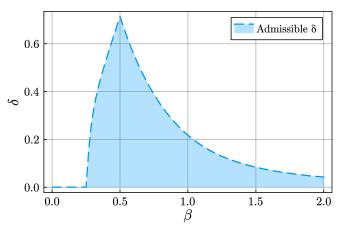
Figure 2: Open set of pairs $(\beta,\delta)$ satisfying Condition 4.4. Condition 4.4 gathers sufficient conditions to ensure Theorem 4.3 on the convergence of the backward Algorithm 2.





4.4 Local linear convergence of three different forward iterations


We address now the question of the linear convergence of Algorithm 2 when we use an approximation $\widehat{{A}}_{k}\approx{A}_{k}$. As before, we examine the convergence rate only for instances for which the algorithm converges. The difference between the forward and the backward case comes from (14), thus depending completely on ${\Theta}_{k}$. Selecting $\widehat{A}_{k}$ where $\|\widehat{{A}}_{k}\|_{2}<\delta$ and replacing $A_{k}$ by $\widehat{A}_{k}$ in (23) yields



(30)

$$\|{\Theta}_{k}\|_{2}\leq\eta\|\widehat{{A}}_{k}-\widehat{{A}}_{k+1}\|_{2}+\mathcal{O}(\|\widehat{{A}}_{k}-\widehat{{A}}_{k+1}\|_{2}^{2}).$$



If we can find $c>0$ (typically $c\geq 1$) such that



(31)

$$\|\widehat{{A}}_{k}-\widehat{{A}}_{k+1}\|_{2}\leq c\|{A}_{k}-{A}_{k+1}\|_{2},$$



the new forward convergence theorem follows directly by replacing $\eta$ by $\widehat{\eta}:=c\eta$ in Theorem 4.3 and Condition 4.4. In practice, (31) means that the approximation $\widehat{A}_{k}$ converges as fast as $A_{k}$ does.
Obtaining $c$ explicitly in (31) happens to be a burden for many approximations $\widehat{{A}}_{k}$. However, ensuring the existence of $c\in[0,+\infty)$ is easier. In the next subsections, we propose three linearly convergent ways of choosing $\widehat{{A}}_{k}$.



4.4.1 The Pure Forward Iteration


The computationally cheapest possible choice for the approximation is $\widehat{{A}}_{k}={A}_{k-1}$, which we term pure forward iteration. In this case, (31) becomes



(32)

$$\|{A}_{k-1}-{A}_{k}\|_{2}\leq c\|{A}_{k}-{A}_{k+1}\|_{2},$$



Equation (32) is reversed when compared to the definition of linear convergence. We will show that (32) holds for $k\in\mathbb{N}$ with the constant



(33)

$$\overline{c}:=\max\left(\sup_{k\in\mathbb{N}}\frac{\|{A}_{k-1}-{A}_{k}\|_{2}}{\|{A}_{k}-{A}_{k+1}\|_{2}},\frac{\|\widehat{{A}}_{0}-{A}_{0}\|_{2}}{\|{A}_{0}-{A}_{1}\|_{2}}\right)\in[0,+\infty).$$



The second argument of the $\max$ is only introduced for Section 4.4.3. Assume there is no static iteration before convergence, i.e., no $k$ such that ${A}_{k}={A}_{k+1}$. The property $\overline{c}\geq 0$ is a direct consequence of its definition. The fact $\overline{c}<+\infty$ holds if and only if there is no super-linear convergence of the sequence $\{\|{A}_{k}-{A}_{k+1}\|_{2}\}_{k\in\mathbb{N}}$ to $0$.
In case this sequence converges super-linearly to $0$, the sequence $\{\|{\Theta}_{k}\|_{2}\}_{k\in\mathbb{N}}$ does too, by (30). Then, ${\Theta}_{k}$ can simply be ignored from our analysis and, we are done. We can thus focus on the case of no super-linear convergence of $\{\|{A}_{k}-{A}_{k+1}\|_{2}\}_{k\in\mathbb{N}}$, which ensures the existence of $\overline{c}\in[0,+\infty)$. The caveat of the pure forward iteration is that we have no control on $\overline{c}$ — that is, on the convergence rate. It is fixed by the system and we can only observe its consequences. This motivates to look for alternative forward iterations.
In the next subsection, we introduce such an alternative, termed pseudo-backward.



Remark 4.5.


For all types of forward iterations, the first estimate $\widehat{{A}}_{0}$ must be chosen heuristically. We propose to compute it using a BCH series expansion in Section 4.5.






4.4.2 The Pseudo-Backward Iteration ($c=1+\nu+\nu\overline{c}_{\nu}$ in (31))


By a pseudo-backward iteration, we mean an iteration scheme where $\widehat{{A}}_{k}$ satifies $\|\widehat{{A}}_{k}-{A}_{k}\|_{2}\leq\nu\|{A}_{k}-{A}_{k-1}\|_{2}$ with $\nu\in[0,1]$. Said otherwise, $\widehat{{A}}_{k}$ ensures a sufficient improvement in each iteration compared to the pure forward approximation ${A}_{k-1}$. This intentionally general definition matches very well all cases where we approximately obtain the backward iterate using an iterative method, for instance Algorithm 3. This is an intermediate type of iteration, designed to converge faster than the forward case without requiring to compute exactly the backward iterate ${A}_{k}$. Notice that $\nu=1$ corresponds to a pure forward iteration while $\nu=0$ corresponds to a backward iteration. This new iteration leads to



(34)

$$\|\widehat{{A}}_{k}-\widehat{{A}}_{k+1}\|_{2}
=\|\widehat{{A}}_{k}-\widehat{{A}}_{k+1}+{A}_{k}-{A}_{k+1}-{A}_{k}+{A}_{k+1}\|_{2}$$






$$\leq\|\widehat{{A}}_{k}-{A}_{k}\|_{2}+\|\widehat{{A}}_{k+1}-{A}_{k+1}\|_{2}+\|{A}_{k+1}-{A}_{k}\|_{2}$$





$$\leq\nu\|{A}_{k}-{A}_{k-1}\|_{2}+\nu\|{A}_{k+1}-{A}_{k}\|_{2}+\|{A}_{k+1}-{A}_{k}\|_{2}$$





$$\leq(1+\nu+\nu\overline{c}_{\nu})\|{A}_{k+1}-{A}_{k}\|_{2},$$



where $\overline{c}_{\nu}$ is defined as in (33), but is affected by $\nu$. The goal here is to enhance the convergence rate by moderating the constant $\overline{c}_{\nu}$ by the adaptive factor $\nu$ such that $1+\nu+\nu\overline{c}_{\nu}\ll\overline{c}$. We design a pseudo-backward algorithm in Section 5.2.




4.4.3 The Accelerated Forward Iteration ($c=\frac{(1+|h|)\overline{c}_{h}}{1-\overline{c}_{h}|h|}$ in (31))


The goal of this third and last type of iteration is to build an improved approximation $\widehat{{A}}_{k}$ using the information encoded in the previous-stage gap ${A}_{k-1}-\widehat{{A}}_{k-1}$ in addition to the knowledge of ${A}_{k-1}$. We define the accelerated forward iteration by $\widehat{{A}}_{k}={A}_{k-1}+h{Q}_{k-1}({A}_{k-1}-\widehat{{A}}_{k-1}){Q}_{k-1}^{T}$ where $h\in\mathbb{R}$ and ${Q}_{k-1}\in\mathrm{O}(p)$.
This new approximant $\widehat{{A}}_{k}$ should be consistent, i.e., the sequence $\{\|\widehat{{A}}_{k}-{A}_{k}\|_{2}\}_{k\in\mathbb{N}}$ should converge linearly to $0$ when $\{\|{A}_{k}-{A}_{k-1}\|_{2}\}_{k\in\mathbb{N}}$ does. This was true by definition in the two previous cases. For the accelerated forward iteration, it follows from




$$\|\widehat{{A}}_{k}-{A}_{k}\|_{2}
\leq\|{A}_{k}-{A}_{k-1}\|_{2}+|h|\|{Q}_{k-1}(\widehat{{A}}_{k-1}-{A}_{k-1}){Q}_{k-1}^{T}\|_{2}$$






$$=\|{A}_{k}-{A}_{k-1}\|_{2}+|h|\|\widehat{{A}}_{k-1}-{A}_{k-1}\|_{2}$$





$$\leq\sum_{l=0}^{k-1}|h|^{l}\|{A}_{k-l}-{A}_{k-1-l}\|_{2}+|h|^{k}\|\widehat{A}_{0}-A_{0}\|_{2}\hskip 54.06006pt\text{(by recursion)}$$





$$\leq\|{A}_{k}-{A}_{k-1}\|_{2}\sum_{l=0}^{k}\overline{c}_{h}^{l}|h|^{l}\hskip 108.12054pt\text{(by \eqref{eq:reversedconvergence} and \eqref{eq:cbar})}$$





$$\leq\frac{1}{1-\overline{c}_{h}|h|}\|{A}_{k}-{A}_{k-1}\|_{2}\hskip 142.26378pt\text{(if $\overline{c}_{h}|h|<1$)}$$



Here, $\overline{c}_{h}$ is defined as in (33) but depends on $h$. Therefore, the accelerated forward iteration is consistent for $h$ small enough. In addition to consistency, $\{\widehat{A}_{k}\}_{k\in\mathbb{N}}$ should be convergent by satisfying (31). It holds since




$$\|\widehat{{A}}_{k+1}-\widehat{{A}}_{k}\|_{2}
=\|{A}_{k}-\widehat{{A}}_{k}+h{Q}_{k}(\widehat{{A}}_{k}-{A}_{k}){Q}_{k}^{T}\|_{2}$$






$$\leq(1+|h|)\|\widehat{{A}}_{k}-{A}_{k}\|_{2}$$





$$\leq\frac{1+|h|}{1-\overline{c}_{h}|h|}\|{A}_{k}-{A}_{k-1}\|_{2}$$





$$\leq\frac{(1+|h|)\overline{c}_{h}}{1-\overline{c}_{h}|h|}\|{A}_{k+1}-{A}_{k}\|_{2}\hskip 113.81102pt\text{(if $\overline{c}_{h}|h|<1$)}$$



Notice that for $h=0$, we retrieve $c=\overline{c}$, the pure forward iteration. Since $\overline{c}_{h}$ continuously depends on $h$ and since $\overline{c}_{h}h=0$ for $h=0$, there is an open neighbourhood of $h=0$ for which $\overline{c}_{h}|h|<1$. The constant $c=\frac{(1+|h|)\overline{c}_{h}}{1-\overline{c}_{h}|h|}$ is worse than $c=\overline{c}$, obtained for the pure forward iteration. This is because a bad step size $h$ can make Algorithm 2 converge slower.


Choosing ${Q}_{k}$ and $h$



We show numerically in Section 5.1 that for $\beta\in[\frac{1}{2},1]$, choosing $h=2\beta-1$ and $Q_{k}=\exp((2\beta-1){A}_{k})$ brings significant speed-up to Algorithm 2. Current attempts to demonstrate theoretically the effectiveness of this choice remained unfruitful due to the several layers of nonlinearity that are involved.







4.5 An efficient start point for the forward iteration


A good initial guess for $\widehat{{A}}_{0}$ is important for the fast convergence of Algorithm 2. Starting from (12) and defining $\log({V}_{0}):=\begin{bmatrix}{E}&-{F}^{T}\\
{F}&{G}\end{bmatrix}\in\mathrm{Skew}(2p)$, the BCH series expansion of the $p\times p$ top-left block of (12) implies that



(35)

$$2\beta({A}_{0}-\widehat{{A}}_{0})={E}-\widehat{{A}}_{0}-\frac{1-2\beta}{12}[{F}^{T}{F},\widehat{{A}}_{0}]-\frac{1-2\beta}{2}[{E},\widehat{{A}}_{0}]+\text{H.O.T.}$$



To obtain a good approximation $\widehat{{A}}_{0}\approx{A}_{0}$, we choose $\widehat{{A}}_{0}$ in such a way that the three first right terms of (35) cancel out. Hence, $\widehat{{A}}_{0}$ must be a solution of the Sylvester equation



(36)

$${S}\widehat{{A}}_{0}+\widehat{{A}}_{0}{S}={E}\text{ where }{S}:=\frac{{I}_{p}}{2}-\frac{1-2\beta}{12}{F}^{T}{F}.$$



If $\beta\geq\frac{1}{2}$, the smallest eigenvalue of $S$ is bounded from below by $\frac{1}{2}$. By [6, Thm. VII.2.12], we have $\|\widehat{A}_{0}\|_{2}\leq\|E\|_{2}\leq\delta$. If $0<\beta<\frac{1}{2}$, the smallest eigenvalue of $S$ is bounded from below by $\frac{1}{2}-\frac{1-2\beta}{12}\delta^{2}$, thus $\|\widehat{A}_{0}\|_{2}\leq\frac{6}{6-(1-2\beta)\delta^{2}}\|E\|_{2}\leq\frac{6\delta}{6-(1-2\beta)\delta^{2}}$.
In this paper, all the experiments are performed using this first initial guess $\widehat{{A}}_{0}$.




4.6 A quasi-geodesic sub-problem for the backward iteration


We have not yet addressed the question of how to perform a backward iteration. Equation (11) has to be solved. Following [3], it can be termed “finding a quasi-geodesic”, stated in Problem 4.6.



Problem 4.6.


Quasi-geodesic sub-problem
Given ${V}\in\mathrm{SO}(2p)$ and $\beta>0$, find ${D}$, ${C}\in\mathrm{Skew}(p),\ {B}\in\mathbb{R}^{p\times p}$ such that



(37)

$$\gamma_{{BCD}}(t):=\exp\left(t\begin{bmatrix}2\beta{D}&-{B}^{T}\\
{B}&{C}\end{bmatrix}\right)\begin{bmatrix}\exp(t(1-2\beta){D})&{0}\\
{0}&{I}_{p}\end{bmatrix}\text{ ends in }\gamma_{{BCD}}(1)={V}.$$







Algorithm 3 is a method to solve Problem 4.6. It is a simplified version of Algorithm 2 where ${C}_{k}$ is not constrained to converge to ${0}$ anymore. Starting from an initial guess $\widehat{D}_{0}$ ($A_{k-1}$ in practice), we successively obtain $D_{k}$ and update $\widehat{D}_{k+1}$ as the accelerated forward approximation of $D_{k+1}$ for $k=0,1,...$. Then, we set $\widehat{A}_{k}=D_{\infty}$ and perform the next backward iteration of Algorithm 2. Solving Problem 4.6 to $\epsilon$-precision using Algorithm 3 is however not competitive with the previously proposed methods [9, 31, 35]. This is why we investigate a pseudo-backward iteration in Section 5.2 — we only perform a few iterations of Algorithm 3 to improve the approximation $\widehat{A}_{k}$. An alternative method to solve Problem 4.6 based on shooting principle from [9] is proposed in Appendix D. In practice, we observed the better performance of Algorithm 3.


Algorithm 3  The sub-problem’s iterative algorithm


1:  INPUT: Given ${V}\in\mathrm{SO}(2p)$, $\widehat{D}_{0}\in\mathrm{Skew}(p)$, $\beta>0$ and $\epsilon>0$, compute:



2:  Define $\tau=1-2\beta$.



3:  for $k=0,1,...$ do





4:     Compute $\begin{bmatrix}2\beta{D}_{k}&-{B}_{k}^{T}\\
{B}_{k}&{C}_{k}\end{bmatrix}=\log\left({V}\begin{bmatrix}\exp(-\tau\widehat{{D}}_{k})&{0}\\
{0}&{I}_{p}\end{bmatrix}\right)$.



5:     if $\|{D}_{k}-\widehat{{D}}_{k}\|_{\mathrm{F}}<\epsilon$ then





6:        break



7:     end if


8:     $\widehat{{D}}_{k+1}={D}_{k}-\tau\exp(-\tau{D}_{k})({D}_{k}-\widehat{{D}}_{k})\exp(\tau{D}_{k})$.



9:  end for


10:  return  ${D}_{k}$








5 The performance of forward iterations


This section investigates the numerical convergence of the different forward iterations introduced in Section 4.4. These variants of Algorithm 2 are benchmarked in Section 6.2.



5.1 The accelerated forward iteration


Section 4.4.3 defined the accelerated forward iteration. Figure 3 quantifies how much this strategy speeds-up Algorithm 2 compared to using the pure forward iteration. First, notice on Figure 3 that the convergence rate of the pure forward iteration is very sensitive to $\beta$. In comparison, the accelerated forward method provides a convergence rate that is almost independent of $\beta$ when it converges. The improvement effect as a function of $\beta$ and $\|\widetilde{U}-U\|_{F}$ is summarized on the bottom right plot of Figure 3. The fast increase of the improvement factor for $\beta=1$ when the Frobenius distance gets larger is due to the increased convergence radius of the accelerated forward iteration, while the pure forward gets close to divergence.









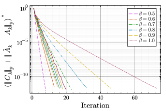
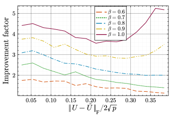
Figure 3: Convergence of Algorithm 2 with an accelerated forward iteration (${Q}_{k}=\exp((2\beta-1){A}_{k})$) from Section 5.1 (solid lines) and the pure forward iteration (stylized lines) on $\mathrm{St}(n=120,p=50)$. The matrices ${U},\widetilde{U}$ are randomly generated at Frobenius distance $\|{U}-\widetilde{U}\|_{\mathrm{F}}\in\{0.03,0.19,0.37\}\cdot 2\sqrt{p}$ for respectively the top left, top right and bottom left plots. The stars “ $*$” on the y-axes specify that the residuals are normalized by the residual of the first iteration. The bottom right figure shows how the improvement factor (i.e., the ratio between the number of iterations of the pure forward and the accelerated forward method) varies as the Frobenius distance increases in $\mathrm{St}(n=60,p=30)$.




5.2 The pseudo-backward iteration compared to the pure forward iteration


Pseudo-backward iterations only perform a few sub-iterations of Algorithm 3 with $\widehat{{D}}_{0}:={A}_{k-1}$ to improve the quality of the estimator $\widehat{A}_{k}$ such that $\|\widehat{A}_{k}-A_{k}\|_{F}\leq\nu\|A_{k-1}-A_{k}\|_{F}$ with $\nu<1$. The left plot of Figure 4 exemplifies that performing two sub-iterations can already provide $\nu\approx 0.1$. Combine this with a second observation: Algorithm 2 produces a new iterate ${A}_{k+1}$ anyway so that it is not worth the computational effort to obtain $\widehat{{A}}_{k}$ with $\|\widehat{{A}}_{k}-{A}_{k}\|_{\mathrm{F}}\ll\|{A}_{k+1}-{A}_{k}\|_{\mathrm{F}}$. Hence, the first iterations of Algorithm 3 speed-up Algorithm 2 but the last ones are a waste of resource. Figure 4 investigates the optimal number of sub-iterations to perform. The further $\beta$ is away from $\frac{1}{2}$, the more the sub-iterations are improving the performance. For $\beta\in\left[\frac{1}{2},1\right]$, the optimal number of sub-iterations settles at $2$.


Figure 5 illustrates that the more sub-iterations of Algorithm 3 are performed, the fewer iterations of Algorithm 2 are needed. For these experiments, 4 sub-iterations are enough to reach the performance of the backward iteration.






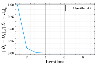
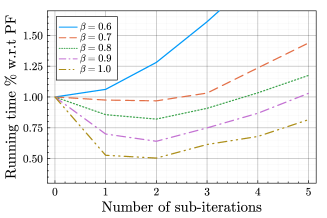
Figure 4: On the left, the evolution of the residual $\|{D}_{k}-\widehat{{D}}_{k}\|_{\mathrm{F}}$ of Algorithm 3 for a random matrix $V\in\mathrm{SO}(40)$ with $\|V-I_{40}\|_{F}=0.32\cdot 2\sqrt{40}$. On the right, the improvement in running time of the pseudo-backward iterations compared to the pure forward (PF) iterations when $\beta$ and the number of sub-iterations vary. The stopping criterion is set to $(\|C_{k}\|_{F}+\|\widehat{A}_{k}-A_{k}\|_{F})^{*}<10^{-12}$. The experiment is performed on $\mathrm{St}(n=40,p=20)$ at distance $\|{U}-\widetilde{U}\|_{\mathrm{F}}=(0.31\pm 0.01)\cdot 2\sqrt{p}$








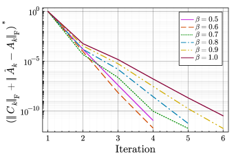
Figure 5: Evolution of the residuals $\|{C}_{k}\|_{\mathrm{F}}+\|{A}_{k}-\widehat{{A}}_{k}\|_{\mathrm{F}}$ for the pure forward iteration (top left) pseudo-backward iteration with 2 sub-iterations (top right) and 4 sub-iterations (bottom) for a random experiment on $\mathrm{St}(n=80,p=30)$ with $\|{U}-\widetilde{U}\|_{\mathrm{F}}=0.16\cdot 2\sqrt{p}\approx 1.75$. The star “ $*$” indicates that the residuals are normalized by the residual of the first iteration.
For all plots, the curve for $\beta=0.5$ (solid purple line) is the same.




6 Performance analysis


We investigate the performance of Algorithm 2 through two questions: how often and how fast does it converge? To answer the first one, we estimate a probabilistic convergence radius— that is, we find the distance $\|{U}-\widetilde{U}\|_{\mathrm{F}}$ such that Algorithm 2 converges with probability close to 1, say 0.99. For the second question, we compare the running times of known methods, carefully implemented to extract the best performance for each of them.



6.1 Probabilistic radius of convergence


From randomized numerical experiments, we fit a logistic model $m_{\theta}(x)\approx P(\text{Alg.~{}\ref{alg:generalizedStiefel} converged}\ |\ \|\widetilde{U}-{U}\|_{\mathrm{F}}=x)$ where $\theta$ is chosen as the maximum likelihood estimator. The details and motivation of this fitting are described in Appendix E. The left plot on Figure 6 displays the fitting models on $\mathrm{St}(32,16)$. This fit provides a probabilistic radius of convergence $r$ by taking $r:=\max\{x\in\mathbb{R}\ |\ m_{\theta}(x)\geq 0.99\}$, i.e., the probability of convergence is higher than $99\%$ if $\|{U}-\widetilde{U}\|_{\mathrm{F}}\leq r$. The right plot on Figure 6 shows that convergence is most challenging under the Euclidean metric ($\beta=1$). In this case, Algorithm 2 converges with high probability if the distance of the inputs is $\|U-\widetilde{U}\|_{F}<0.4\cdot 2\sqrt{p}$.






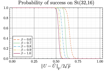
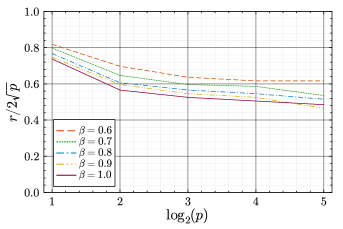
Figure 6: On the left, the logistic regression models on 1000 random samples on $\mathrm{St}(32,16)$. The models are trained until $\|\nabla f(\theta)\|_{F}<10^{-8}$ (see Appendix E). The logistic model estimates the probability of success of Algorithm 2 (implemented with 2 pseudo-backward sub-iterations). For $\beta$ from $0.6$ to $1$, the R2 factors of the fitting are $\{0.85,0.97,0.96,0.98,0.97\}$, confirming the goodness of fit. On the right, the evolution of the radius of convergence as $p$ varies.



Remark 6.1.


When ${U},\widetilde{U}$ are not in the convergence radius of Algorithm 2, it is still possible to use it as a subroutine for a globally convergent method, e.g., the leapfrog method of [26]. This method has already been considered on the Stiefel manifold [31, 32]. It was then combined with the shooting method. However, being a global method, the leapfrog method needs not to be used inside the convergence radius of Algorithm 2.






6.2 Benchmark


We benchmark the different versions of Algorithm 2 with the $p$-shooting method [35, Algorithm 2]. The benchmarking is performed on random matrices $\operatorname{\mathit{U}}_{i},\operatorname{\mathit{\widetilde{U}}}_{i}\in\mathrm{St}(n,p)$ for $i=1,...,N$ generated at fixed Frobenius distance. In view of the homogeneity of $\mathrm{St}(n,p)$, the $U_{i}$’s can be chosen arbitrarily w.l.o.g, here by applying a Gram-Schmidt process on a random matrix. The $\operatorname{\mathit{\widetilde{U}}}_{i}$’s are built within the convergence radius as follows. For ${A}_{i}\in\mathrm{Skew}(n)$ filled with i.i.d normally distributed entries $\sim\mathcal{N}(0,\delta)$, we build $\operatorname{\mathit{\widetilde{U}}}_{i}=[\operatorname{\mathit{U}}_{i}\ \operatorname{\mathit{U}}_{i,\perp}]\exp({A}_{i}){I}_{n\times p}$. Because of a “Central Limit Theorem effect”, if $\delta$ is fixed and $n,p$ are large, the value of $\frac{\|\operatorname{\mathit{U}}_{i}-\operatorname{\mathit{\widetilde{U}}}_{i}\|_{\mathrm{F}}^{2}}{4p}\in[0,1]$ converges to a mean. Our experiments compare


 

Algorithm 2 using pure forward iterations.



 

Algorithm 2 using pseudo-backward iterations with 1 and 2 sub-iterations of Algorithm 3.



 

Algorithm 2 using accelerated forward iterations.



 

The $p$-shooting method [35, Algorithm 2] with 3 and 5 discretization points, implemented as in RiemannStiefelLog.



We consider two sizes of Stiefel manifolds, $\mathrm{St}(80,20)$ (Tables 1 and 2) and $\mathrm{St}(100,50)$ (Table 3). We also consider two distances between the samples, expressed in percentage of the Frobenius diameter of $\mathrm{St}(n,p)$ ($=2\sqrt{p}$). We consider $15\%$ (Table 1) and $32\%$ (Tables 2 and 3). Given a method $M$ that ran $T$ times with CPU times $t_{M,j}(\operatorname{\mathit{U}}_{i},\operatorname{\mathit{\widetilde{U}}}_{i})$ for $j=1,\ldots,T$, the running time $t_{M}$ of the method $M$ is computed as follows.



(38)

$$t_{M}=\frac{1}{N}\sum_{i=1}^{N}\min_{j=1,...,T}t_{M,j}(\operatorname{\mathit{U}}_{i},\operatorname{\mathit{\widetilde{U}}}_{i}).$$



The “$\min$” in (38) is more standard than the average for benchmarking, as implemented for the @btime macro in Julia [5].
For Tables 1, 2 and 3, we take $N=T=10$. The experiments from Tables 1, 2 and 3 demonstrate the effectiveness of Algorithm 2 compared to the shooting method for $\beta\in[0.3,1]$. The shooting method is only competetive with Algorithm 2 when $\beta=1$, i.e., in the case of the Euclidean metric. In particular the accelerated forward iteration appears to be the best choice since it is very close in performance to the other types of iterations in case $\beta\leq\frac{1}{2}$ and outperforms them otherwise.



7 Conclusion


In this paper, we have proposed an alternative method to the shooting method to compute a geodesic between any two points on the Stiefel manifold. The method generalizes the approach of [34] to the complete family of metrics introduced in [18]. Our analysis included theoretical guarantees and numerical experiments. Future work may include the design of a more robust initialisation, increasing significantly the current restrictive radius of convergence. A more detailed understanding of the effectiveness of the accelerated forward iteration should also be carried out.





$\mathrm{St}(80,20),\quad\|{U}-\widetilde{U}\|_{\mathrm{F}}=(0.15\pm 0.01)\cdot 2\sqrt{p}$




$\beta$
0.3
0.4
0.5
0.6
0.7
0.8
0.9
1


Scale
$\cdot 10^{-2}s$


Pure Forward
2.8
1.0
0.31
0.84
1.1
1.35
1.6
1.8


Pseudo-Backward 1 it.
1.5
0.93
0.31
0.76
0.86
0.92
0.88
0.89


Pseudo-Backward 2 it.
1.35
0.85
0.31
0.85
0.84
0.85
0.86
0.93


Acc. Forward
1.30
0.87
0.31
0.79
0.81
0.85
0.81
0.80


p-shooting 3 pt.
2.3
2.1
1.8
1.8
1.5
1.3
15(x)
0.92


p-shooting 5pt
2.9
2.7
2.2
2.2
2.0
1.8
1.4
1.2



Table 1: Benchmark of Algorithm 2 in its different versions (pure forward, pseudo-backward with 1 or 2 sub-iterations and accelerated forward). It is compared to the $p$-shooting method [35, Algorithm 2] with $3$ and $5$ points (starting and ending point included). With only $3$ points, the apparition of failures (x) indicates that more points must be considered for robustness.





$\mathrm{St}(80,20),\quad\|{U}-\widetilde{U}\|_{\mathrm{F}}=(0.32\pm 0.01)\cdot 2\sqrt{p}$




$\beta$
0.3
0.4
0.5
0.6
0.7
0.8
0.9
1


Scale
$\cdot 10^{-2}s$


Pure Forward
3.3
1.2
0.44
0.95
1.2
1.6
1.9
2.2


Pseudo-Backward 1 it.
2.7
1.3
0.45
1.1
1.2
1.3
1.5
1.6


Pseudo-Backward 2 it.
2.6
1.4
0.42
1.4
1.4
1.3
1.5
1.6


Acc. Forward
2.7
1.3
0.45
1.1
1.3
1.3
1.3
1.3


p-shooting 3 pt.
4.3
3.8
2.8
2.8
2.4
17(x)
1.7
1.6


p-shooting 5pt
5.3
4.6
3.6
3.4
2.9
2.6
2.3
1.8



Table 2: Same as Table 1 with $\|\widetilde{U}-U\|_{F}=(0.32\pm 0.01)\cdot 2\sqrt{p}$.





$\mathrm{St}(100,50),\quad\|{U}-\widetilde{U}\|_{\mathrm{F}}=(0.32\pm 0.01)\cdot 2\sqrt{p}$




$\beta$
0.3
0.4
0.5
0.6
0.7
0.8
0.9
1


Scale
$\cdot 10^{-1}s$


Pure Forward
5.2
1.8
0.71
1.5
2.1
3.0
4.3
7.4


Pseudo-Backward 1 it.
5.6
1.6
0.72
1.4
1.7
1.9
2.0
2.1


Pseudo-Backward 2 it.
5.8
1.8
0.71
1.5
1.7
1.7
1.9
1.9


Acc. Forward
8.1
1.9
0.72
1.4
1.7
1.7
1.6
1.7


p-shooting 3 pt.
38(x)
5.1
12(x)
3.1
2.5
33(x)
1.6
22(x)


p-shooting 5pt
18(x)
5.5
3.5
3.3
2.6
2.1
1.9
1.6



Table 3: Same as Table 1 with $\|\widetilde{U}-U\|_{F}=(0.32\pm 0.01)\cdot 2\sqrt{p}$ on $\mathrm{St}(100,50)$. Here, $3$ points are clearly not enough for the shooting method given its numerous failures (x).




Appendix A Rank of logarithm


Given $U,\widetilde{U}\in\mathrm{St}(n,p)$, we investigate the cases where $\Delta\in\mathrm{Log}_{\beta,{U}}(\widetilde{U})$ and



(39)

$$\mathrm{rank}(({I}-{U}{U}^{T})\Delta)>\mathrm{rank}(({I}-{U}{U}^{T})\widetilde{U}).$$



An example where (39) holds is for antipodal points ($\widetilde{U}=-U$) on the hypersphere $\mathrm{St}(n,1)$. We show that (39) can only happen when $\widetilde{U}$ belongs to the cut locus of $U$, which is a zero-measure subset of $\mathrm{St}(n,p)$ [29, Lemma 4.4].



Proposition A.1.


Assume $U,\widetilde{U}\in\mathrm{St}(n,p)$ and (39) holds. Then $\widetilde{U}$ belongs to the cut locus of $U$.





Proof A.2.


Assume $\Delta\in\mathrm{Log}_{\beta,U}(\widetilde{U})$. By definition, we can always write $\Delta=UA+\begin{bmatrix}Q_{1}&Q_{2}\end{bmatrix}\begin{bmatrix}B_{1}\\
B_{2}\end{bmatrix}$ where $\mathrm{col}([U\ Q_{1}])=\mathrm{col}([U\ \widetilde{U}])$ and $Q_{2}^{T}U=Q_{2}^{T}\widetilde{U}=0$. By the assumption (39), we have $Q_{2},B_{2}\neq 0$. Let $Q_{2}\in\mathrm{St}(n,q)$ with $q\geq 1$. Then, we have




$$\widetilde{U}
=\mathrm{Exp}_{\beta,U}(\Delta)$$





$$\iff\begin{bmatrix}U^{T}\widetilde{U}\\
Q_{1}^{T}\widetilde{U}\\
0\end{bmatrix}
=\exp\begin{bmatrix}2\beta A&\begin{matrix}-{B}_{1}^{T}&-{B}_{2}^{T}\end{matrix}\\
\begin{matrix}{B}_{1}\\
{B}_{2}\end{matrix}&{0}_{n-p}\end{bmatrix}I_{n\times p}\exp((1-2\beta)A)$$





$$\iff\begin{bmatrix}U^{T}\widetilde{U}\\
Q_{1}^{T}\widetilde{U}\\
0\end{bmatrix}
=\exp\begin{bmatrix}2\beta A&\begin{matrix}-{B}_{1}^{T}&-(R{B}_{2})^{T}\end{matrix}\\
\begin{matrix}{B}_{1}\\
R{B}_{2}\end{matrix}&{0}_{n-p}\end{bmatrix}I_{n\times p}\exp((1-2\beta)A)\text{ for all }R\in\mathrm{O}(q).$$




Therefore, for all $R\in\mathrm{O}(q)$ and $\widetilde{\Delta}:=UA+\begin{bmatrix}Q_{1}&Q_{2}\end{bmatrix}\begin{bmatrix}B_{1}\\
RB_{2}\end{bmatrix}$, $\mathrm{Exp}_{\beta,U}(\widetilde{\Delta})=\widetilde{U}$ and $\|\widetilde{\Delta}\|_{\beta}=\|\Delta\|_{\beta}$ yield $\widetilde{\Delta}\in\mathrm{Log}_{\beta,U}(\widetilde{U})$. In conclusion, there is more than one minimal geodesic from $U$ to $\widetilde{U}$ and $\widetilde{U}$ is on the cut locus of $U$ by [29, Proposition 4.1].






Appendix B Initialization of $V_{0}$



Both Algorithms 1 and 2 ask for an initialization $V_{0}=\begin{bmatrix}M&O\\
N&P\end{bmatrix}\in\mathrm{SO}(2p)$. $M=U^{T}\widetilde{U}$ is fixed by the problem. However, $N$, $O$, $P$ and $Q$ have degrees of freedom to obtain the best performance. Let us recall their meaning. From Theorem 2.1, we know that for $n\leq 2p$, the geodesic can be considered as a curve evolving in $\mathrm{St}(n,2p)$, from which we only retain the $p$ first columns. In $\mathrm{St}(n,2p)$, the geodesic starts at $[U\ Q]$ and ends at $[\widetilde{U}\ \widetilde{Q}]$. The underlying goal of Algorithms 1 and 2 is to obtain $Q,\widetilde{Q}\in\mathrm{St}(n,p)$ minimizing the distance from $[U\ Q]$ to $[\widetilde{U}\ \widetilde{Q}]$. From this framework, $V_{0}$ can be interpreted as



(40)

$$V_{0}:=\begin{bmatrix}U^{T}\widetilde{U}&U^{T}\widetilde{Q}\\
Q^{T}\widetilde{U}&Q^{T}\widetilde{Q}\end{bmatrix}\in\mathrm{SO}(2p).$$



A heuristic initialization is finding $Q,\widetilde{Q}$ minimizing the geodesic distance $d(I,V_{0})$ in $\mathrm{SO}(2p)$. It is known that $d(I,V_{0})\propto\|\log(V_{0})\|_{F}$ (see, e.g., [13]). Since $U,\widetilde{U}$ are fixed, an easier problem is to solve $\min_{Q,\widetilde{Q}}\|I-Q^{T}\widetilde{Q}\|_{F}$. The column spaces of $Q,\widetilde{Q}$ are known. This second problem is thus an Orthogonal Procrustes problem, solved by the SVD. It admits an infinite set of solutions, given by all orthogonal similarity transformations of $Q^{T}\widetilde{Q}$. Let us build these solutions. If we take $\widehat{Q}\widehat{N}=(I-UU^{T})\widetilde{U}$ (with $\widehat{Q}\in\mathrm{St}(n,p)$ and $\widehat{Q}^{T}U=0$), we can start with any $\begin{bmatrix}M&\widehat{O}\\
\widehat{N}&\widehat{P}\end{bmatrix}\in\mathrm{SO}(2p)$. The idea from [34] is to compute $\widehat{P}=R\Sigma\widetilde{R}^{T}$, a singular value decomposition.


 

Method from [34]: take $Q:=\widehat{Q}$, $N:=\widehat{N}$, $O:=\widehat{O}\widetilde{R}R^{T}$, $P=R\Sigma R^{T}$.



 

Our method: take $Q:=\widehat{Q}R$, $N=R^{T}\widehat{N}$, $O=\widehat{O}\widetilde{R}$, $P=\Sigma$.



Our method corresponds to a similarity transformation of the method from [34] by $\begin{bmatrix}I&0\\
0&R\end{bmatrix}$. It offers a diagonal matrix $P$.




Appendix C Intermediate results for Section 4.3



This appendix gathers intermediate results in the proof of Theorem 4.3. It allows to keep a clear narration in Section 4.3.
First, Lemma 1 allows to relate the norm of two matrices appearing in Theorem 4.3.



Lemma 1.


Let ${L}_{k}:=\begin{bmatrix}{A}_{k}&-{B}_{k}^{T}\\
{B}_{k}&{C}_{k}\end{bmatrix}$ and ${X}_{k}:=\begin{bmatrix}2\beta{A}_{k}&-{B}_{k}^{T}\\
{B}_{k}&{C}_{k}\end{bmatrix}$
produced by Algorithm 2, then $\|{X}_{k}\|_{2}\leq(1+|2\beta-1|)\|{L}_{k}\|_{2}$ and $\|{L}_{k}\|_{2}\leq\left(1+\frac{|2\beta-1|}{2\beta}\right)\|{X}_{k}\|_{2}$.





Proof C.1.


Simply notice that




$$X_{k}=L_{k}+\begin{pmatrix}(2\beta-1)A_{k}&0\\
0&0\end{pmatrix}\Rightarrow\|X_{k}\|_{2}\leq\|L_{k}\|_{2}+|2\beta-1|\|L_{k}\|_{2},$$



and




$$L_{k}=X_{k}+\begin{pmatrix}(1-2\beta)A_{k}&0\\
0&0\end{pmatrix}\Rightarrow\|L_{k}\|_{2}\leq\|X_{k}\|_{2}+\frac{|2\beta-1|}{2\beta}\|X_{k}\|_{2}.$$



This concludes the proof.




Then, Lemma 2 allows to bound the higher order terms from (23) in terms of the norm of $\|A_{k}-A_{k+1}\|_{2}$.



Lemma 2.


In (23), we can bound the higher order terms by $\|\mathrm{H.O.T}_{\Theta}(4)\|_{2}\leq|\tau|(|\tau|\delta)^{2}\log\left(\frac{1}{1-2|\tau|\delta}\right)\|A_{k}-A_{k+1}\|_{2}$.





Proof C.2.


We know from the commutator version of the Goldberg series [23] (or BCH formula) that




$$\|\mathrm{H.O.T}_{\Theta}(4)\|_{2}\leq\sum_{\ l=4}^{\infty}\sum_{w_{l}}\frac{|g_{w_{l}}|}{l}\|[w_{l}(\tau A_{k},\tau A_{k+1})]\|_{2}$$



where $w_{l}(\tau A_{k},\tau A_{k+1})$ is a word of length $l$ in the alphabet $\{\tau A_{k},\tau A_{k+1}\}$ and $[w_{l}(\tau A_{k},\\
\tau A_{k+1})]$, $[w_{l}]$ for short, is the extended commutator defined on this word [23]. $g_{w_{l}}$ is the Goldberg coefficient associated to $w_{l}$ [16]. Since $\|[A,B]\|_{2}\leq 2\|A\|_{2}\|B\|_{2}$ and $\|[A,B]\|\leq 2\|A\|_{2}\|B-A\|_{2}$, it follows by recurrence that $\|[w_{l}]\|_{2}\leq 2^{l-1}\delta^{l-1}\tau^{l}\|A_{k}-A_{k+1}\|_{2}$. Moreover, for words of length $l$, we have $\sum_{w_{l}}\frac{|g_{w_{l}}|}{l}\leq\frac{2}{l}$ [33]. [34, Lem. A.1] even decreased this bound to $\frac{1}{l}$. It follows that




$$\|\mathrm{H.O.T}_{\Theta}(4)\|_{2}
\leq\sum_{l=4}^{\infty}\sum_{w_{l}}\frac{|g_{w_{l}}|}{l}2^{l-1}\delta^{l-1}\tau^{l}\|A_{k}-A_{k+1}\|_{2}$$






$$\leq|\tau|(|\tau|\delta)^{2}\|A_{k}-A_{k+1}\|_{2}\sum_{l=1}^{\infty}(2|\tau|\delta)^{l}\left(\sum_{w_{l+3}}\frac{|g_{w_{l+3}}|}{l+3}\right)$$





$$\leq|\tau|(|\tau|\delta)^{2}\|A_{k}-A_{k+1}\|_{2}\sum_{l=1}^{\infty}\frac{(2|\tau|\delta)^{l}}{l}$$





$$\leq|\tau|(|\tau|\delta)^{2}\log\left(\frac{1}{1-2|\tau|\delta}\right)\|A_{k}-A_{k+1}\|_{2},$$



where $2|\tau|\delta<1$ stands by Condition 4.4.




Lemma 3 shows that it is indeed valid to go
from (24) to (25) in the proof of Theorem 4.3.



Lemma 3.


Equation (25) follows from (24).





Proof C.3.


The top-left $p\times p$ block of the BCH series expansion of ${A}_{k+1}$ based on the fundamental equation (13) yields





(41)

$$2\beta({A}_{k+1}-{A}_{k})
={\Theta}_{k}+\beta[{A}_{k},{\Theta}_{k}]$$






$$+\frac{1}{12}\Big{(}4\beta^{2}[{A}_{k},[{A}_{k},{\Theta}_{k}]]-{B}_{k}^{T}{B}_{k}{\Theta}_{k}-{\Theta}_{k}{B}_{k}^{T}{B}_{k}+2{B}_{k}^{T}{\Gamma}_{k}{B}_{k}$$





$$-2\beta[{\Theta}_{k},[{A}_{k},{\Theta}_{k}]]\Big{)}-\frac{1}{24}\Big{(}2[{\Theta}_{k},{B}_{k}^{T}{\Gamma}_{k}{B}_{k}]\Big{)}+\mathcal{O}(\|{A}_{k}-{A}_{k+1}\|_{2}^{2})$$





$$+\text{H.O.T}_{{A}}(5).$$



Equation (41) features many terms that we tackle one by one. All the terms can be bounded by leveraging (24) and $\|\Gamma_{k}\|_{2}\leq\frac{6}{6-\delta^{2}}\|C_{k}\|_{2}\leq\frac{6\delta}{6-\delta^{2}}$ [35]:




$$\|[{A}_{k},{\Theta}_{k}]\|_{2}
\leq 2\|{A}_{k}\|_{2}\|{\Theta}_{k}\|_{2}$$






$$\leq 2\delta\eta\|{A}_{k}-{A}_{k+1}\|_{2}+\mathcal{O}(\|{A}_{k}-{A}_{k+1}\|_{2}^{2}),$$




$$\|[{A}_{k},[{A}_{k},{\Theta}_{k}]]\|_{2}
\leq 2\|{A}_{k}\|_{2}\|[{A}_{k},{\Theta}_{k}]\|_{2}$$






$$\leq 4\delta^{2}\eta\|{A}_{k}-{A}_{k+1}\|_{2}+\mathcal{O}(\|{A}_{k}-{A}_{k+1}\|_{2}^{2}),$$




$$\|{B}_{k}^{T}{B}_{k}{\Theta}_{k}\|_{2}
\leq\delta^{2}\eta\|{A}_{k}-{A}_{k+1}\|_{2}+\mathcal{O}(\|{A}_{k}-{A}_{k+1}\|_{2}^{2}),$$





$$\|{B}_{k}^{T}{\Gamma}_{k}{B}_{k}\|_{2}
\leq\frac{6\delta^{2}}{6-\delta^{2}}\|{C}_{k}\|_{2},$$





$$\|[{\Theta}_{k},[{A}_{k},{\Theta}_{k}]]\|
=\mathcal{O}(\|{A}_{k}-{A}_{k+1}\|_{2}^{2}),$$





$$\|[{\Theta}_{k},{B}_{k}^{T}{\Gamma}_{k}{B}_{k}]\|_{2}
\leq 2\delta^{2}\|{\Gamma}_{k}\|_{2}\|{\Theta}_{k}\|_{2}$$






$$\leq\frac{12\delta^{3}}{6-\delta^{2}}\eta\|{A}_{k}-{A}_{k+1}\|_{2}+\mathcal{O}(\|{A}_{k}-{A}_{k+1}\|_{2}^{2}).$$



Inserting all these terms in (41) yields (25).






Appendix D An alternative algorithm to solve Problem 4.6



Algorithm 4 proposes a shooting method on $\mathrm{SO}(2p)$ to solve Problem 4.6, inspired from [9, Algorithm 1]. Notice that the initial shooting direction is ${M}:=\dot{\gamma}_{{BCD}}(0)=\begin{bmatrix}{D}&-{B}^{T}\\
{B}&{C}\end{bmatrix}$. Starting from an initial guess for ${M}_{0}=\dot{\gamma}_{{B_{0}C_{0}D_{0}}}(0)$, ${M}_{k}$ is updated using an approximate parallel transport of the error vector $\operatorname{\Delta}_{k}:={V}-\gamma_{{B_{k}C_{k}D_{k}}}(1)$ along the curve $\gamma_{{B_{k}C_{k}D_{k}}}$. We follow the method of [9, Algorithm 1] to approximate this parallel transport of $\operatorname{\Delta}_{k}$ to the tangent space of $\gamma_{{B_{k}C_{k}D_{k}}}(0)={I}_{2p}$, written $T_{{{I}_{2p}}}\mathrm{SO}(2p)$: $\operatorname{\Delta}_{k}$ is sequentially projected on $T_{\gamma_{{B_{k}C_{k}D_{k}}}(t)}\mathrm{SO}(2p)$ for $t\in[t_{m},t_{m-1},...,t_{1}]$ with $t_{m}$=1 and $t_{1}=0$. The pseudo-code of the method is provided in Algorithm 4.


Algorithm 4  The subproblem’s shooting algorithm


1:  INPUT: Given ${V}\in\mathrm{SO}(2p)$, $\beta>0$, $\epsilon>0$ and $[t_{1},t_{2},...,t_{m}]$ with $t_{1}=0$ and $t_{m}=1$.



2:  Initialize ${M}_{0}:=\begin{bmatrix}{D}_{0}&-{B}_{0}^{T}\\
{B}_{0}&{C}_{0}\end{bmatrix}$ and $k=0$.



3:  while $\nu>\epsilon$ do





4:     for $j=m,m-1,...,1$ do





5:        ${V}^{s}\leftarrow\exp\left(t_{j}\begin{bmatrix}2\beta{D}_{k}&-{B}_{k}^{T}\\
{B}_{k}&{C}_{k}\end{bmatrix}\right)\exp\left(t_{j}\begin{bmatrix}(1-2\beta){D}_{k}&{0}\\
{0}&{0}\end{bmatrix}\right)$



6:        if $j==m$ then





7:           ${W}\leftarrow{V}-{V}^{s}$



8:           $\nu\leftarrow\|{\Delta}\|_{\mathrm{F}}$



9:        end if


10:        ${M}^{s}\leftarrow\mathrm{skew}(({V}^{s})^{T}{W})$                                   #Project ${W}$ on $T_{{V}^{s}}\mathrm{SO}(2p)$.



11:        ${W}\leftarrow{V}^{s}{M}^{s}\cdot\frac{\nu}{\|{M}^{s}\|_{\mathrm{F}}}$



12:     end for


13:     ${M}_{k}\leftarrow{M}_{k}+{M}^{s}$, $k=k+1$.



14:  end while


15:  return  ${D}_{k}$







Appendix E Logistic model fitting


We obtain a probabilistic radius of convergence of Algorithm 2 from numerical experiments. First, define a function $\mathcal{X}_{\beta}:\mathrm{St}(n,p)\times\mathrm{St}(n,p)\mapsto\{0,1\}$ where




$$\mathcal{X}_{\beta}({U},\widetilde{U})=\begin{cases}1\text{ if Algorithm~{}\ref{alg:generalizedStiefel} converged with $({U},\widetilde{U},\beta)$ as input.}\\
0\text{ otherwise.}\end{cases}$$



Given $\beta>0$ and $N$ samples $\{\operatorname{\mathit{U}}_{i},\operatorname{\mathit{\widetilde{U}}}_{i}\}_{i\in\{1...,N\}}$ drawn from a continuous distribution on $\mathrm{St}(n,p)$, we can then build a data set of pairs




$$\{x_{i},y_{i}\}_{i\in\{1...,N\}}:=\{\|\operatorname{\mathit{U}}_{i}-\operatorname{\mathit{\widetilde{U}}}_{i}\|_{\mathrm{F}},\ \mathcal{X}_{\beta}(\operatorname{\mathit{U}}_{i},\operatorname{\mathit{\widetilde{U}}}_{i})\}_{i\in\{1...,N\}}.$$



We expect Algorithm 2 to converge when $\|\operatorname{\mathit{U}}_{i}-\operatorname{\mathit{\widetilde{U}}}_{i}\|_{\mathrm{F}}$ is small and failures to appear when $\|\operatorname{\mathit{U}}_{i}-\operatorname{\mathit{\widetilde{U}}}_{i}\|_{\mathrm{F}}$ gets larger. This framework is natural to fit a logistic regression model $m_{\theta}:\mathbb{R}\mapsto(0,1):x\mapsto m_{\theta}(x)$, where $\theta:=(\theta_{0},\ \theta_{1})\in\mathbb{R}^{2}$ is the fitting parameter. The goodness of fit is confirmed by the high coefficients of determination $R^{2}$ provided in Figure 6. The model predicts the probability of convergence of Algorithm 2. It is given by




$$m_{\theta}(x)=\frac{1}{1+\exp(\theta_{0}+\theta_{1}x)}.$$



The estimator $\theta$ is chosen to maximize the likelihood of the data set, i.e.,




$$\theta:=\mathrm{argmax}_{\theta\in\mathbb{R}^{2}}\prod_{i=1}^{N}m_{\theta}(x_{i})^{y_{i}}(1-m_{\theta}(x_{i}))^{(1-{y_{i}})}.$$



It is well-known that it is easier and equivalent to obtain the log-likelihood estimator



(42)

$$\theta:=\mathrm{argmax}_{\theta\in\mathbb{R}^{2}}f(\theta):=\mathrm{argmax}_{\theta\in\mathbb{R}^{2}}\sum_{i=1}^{N}\log(m_{\theta}(x_{i}))y_{i}+\log(1-m_{\theta}(x_{i}))(1-{y_{i}}).$$



Equation (42) is a Lipschitz-smooth convex optimization problem and is solved using the accelerated gradient method [22] with stopping criterion $\|\nabla f(\theta)\|_{\mathrm{F}}<10^{-8}$. We considered $N=1000$ in our experiments.

References

[1]
Absil, P.-A., Mahony, R., Sepulchre, R.: Optimization Algorithms on
Matrix Manifolds. Princeton University Press, Princeton, NJ (2008)
[2]
Absil, P.-A.., Mataigne, S.: The ultimate upper bound on the
injectivity radius of the Stiefel manifold (2024)
[3]
Bendokat, T., Zimmermann, R.: Efficient quasi-geodesics on the Stiefel
manifold. Lecture Notes in Computer Science pp. 763–771 (2021)
[4]
Bergmann, R.: Manopt.jl: Optimization on manifolds in Julia. Journal of Open
Source Software 7(70), 3866 (2022). 10.21105/joss.03866
[5]
Bezanson, J., Edelman, A., Karpinski, S., Shah, V.B.: Julia: A fresh approach
to numerical computing. SIAM review 59(1), 65–98 (2017),
https://doi.org/10.1137/141000671
[6]
Bhatia, R.: Matrix Analysis, vol. 169. Springer (1997)
[7]
Boumal, N., Mishra, B., Absil, P.-A., Sepulchre, R.: Manopt, a
Matlab toolbox for optimization on manifolds. Journal of Machine Learning
Research 15(42), 1455–1459 (2014), https://www.manopt.org
[8]
Brigant, A.L., Puechmorel, S.: Quantization and clustering on Riemannian
manifolds with an application to air traffic analysis. Journal of
Multivariate Analysis 173, 685–703 (2019).
10.1016/j.jmva.2019.05.008
[9]
Bryner, D.: Endpoint Geodesics on the Stiefel Manifold Embedded in
Euclidean space. SIAM Journal on Matrix Analysis and Applications
38(4), 1139–1159 (2017). 10.1137/16M1103099,
https://doi.org/10.1137/16M1103099
[11]
Chakraborty, R., Vemuri, B.C.: Statistics on the Stiefel manifold: Theory and
applications. The Annals of Statistics 47(1), 415 – 438 (2019)
[12]
Cheeger, J.: Some examples of manifolds of nonnegative curvature. Journal of
Differential Geometry 8(4), 623–628 (Dec 1973).
10.4310/jdg/1214431964
[14]
Fréchet, M.R.: Les éléments aléatoires de nature quelconque dans un
espace distancié. Annales de l’institut Henri Poincaré 10(4),
215–310 (1948)
[15]
Gao, B., Vary, S., Ablin, P., Absil, P.-A.: Optimization flows landing
on the Stiefel manifold. IFAC-PapersOnLine 55(30), 25–30
(2022),
https://www.sciencedirect.com/science/article/pii/S2405896322026519,
25th IFAC Symposium on Mathematical Theory of Networks and Systems MTNS 2022
[17]
Huang, L., Liu, X., Lang, B., Yu, A., Wang, Y., Li, B.: Orthogonal weight
normalization: Solution to Optimization over multiple dependent Stiefel
Manifolds in Deep Neural Networks. Proceedings of the AAAI Conference
on Artificial Intelligence 32(1) (Apr 2018),
https://ojs.aaai.org/index.php/AAAI/article/view/11768
[19]
Jung, S., Dryden, I., Marron, J.S.: Analysis of principal nested spheres.
Biometrika 99(3), 551–568 (2012). 10.1093/biomet/ass022
[20]
Kent, J., Hamelryck, T.: Using the Fisher-Bingham distribution in stochastic
models for protein structure. Quantitative Biology, Shape Analysis, and
Wavelets 24(1), 57–60 (2005)
[21]
Miolane, N., Guigui, N., Brigant, A.L., Mathe, J., Hou, B., Thanwerdas, Y.,
Heyder, S., Peltre, O., Koep, N., Zaatiti, H., Hajri, H., Cabanes, Y.,
Gerald, T., Chauchat, P., Shewmake, C., Brooks, D., Kainz, B., Donnat, C.,
Holmes, S., Pennec, X.: Geomstats: A Python Package for Riemannian
Geometry in Machine Learning. Journal of Machine Learning Research
21(223), 1–9 (2020), http://jmlr.org/papers/v21/19-027.html
[22]
Nesterov, Y.: A method for solving the convex programming problem with
convergence rate O(1/(k*k)). Proceedings of the USSR Academy of
Sciences 269, 543–547 (1983)
[23]
Newman, M., Thompson, R.C.: Numerical values of Goldberg’s coefficients in
the series for . Mathematics of Computation 48(177),
265–s132 (1987), http://www.jstor.org/stable/2007889
[24]
Nguyen, D.: Curvatures of Stiefel manifolds with deformation metrics. Journal
of Lie Theory 32(2), 563–600 (2022)
[26]
Noakes, L.: A global algorithm for geodesics. Journal of the Australian
Mathematical Society. Series A. Pure Mathematics and Statistics
65(1), 37–50 (1998). 10.1017/S1446788700039380
[27]
Pennec, X., Fillard, P., Ayache, N.: A Riemannian Framework for Tensor
Computing. International Journal of Computer Vision 66(1), 41–66
(1 2006)
[30]
Stoye, J., Zimmermann, R.: On the injectivity radius of the Stiefel manifold:
Numerical investigations and an explicit construction of a cut point at short
distance (2024)
[31]
Sutti, M.: Shooting methods for computing geodesics on the stiefel manifold
(2023)
[32]
Sutti, M., Vandereycken, B.: The leapfrog algorithm as nonlinear
Gauss-Seidel (2023)
[34]
Zimmermann, R.: A Matrix-Algebraic Algorithm for the Riemannian
Logarithm on the Stiefel Manifold under the Canonical Metric. SIAM
Journal on Matrix Analysis and Applications 38(2), 322–342
(2017). 10.1137/16M1074485, https://doi.org/10.1137/16M1074485
[35]
Zimmermann, R., Hüper, K.: Computing the Riemannian Logarithm on the
Stiefel Manifold: Metrics, Methods, and Performance. SIAM Journal
on Matrix Analysis and Applications 43(2), 953–980 (2022).
10.1137/21M1425426, https://doi.org/10.1137/21M1425426