Controller to eliminate the first harmonic in delayed periodic signal with application to rotational scanning atomic force microscopy

Abstract

The plant (system to be controlled) produces a periodic signal containing broad spectrum of the Fourier harmonics. The first Fourier harmonic (sine-type signal) assumed to be undesirable and should be removed by an external force, while other harmonics should be preserved. Because the measured plant data has an unknown amount of time delay and a sensitivity of the plant to external force is unknown, thus the amplitude and the phase of an anti-sine control force are unknown as well. We developed an adaptive controller described as a linear time-invariant system which is able to remove the first harmonic from the plant’s output by constantly adjusting it’s parameters of control force even if time delay of the plant output signal and plant sensitivity to the external force have slow variations over time. That type of controller was requested to further extend capabilities of newly developed high-speed large-area rotational scanning atomic force microscopy technique where the sample is rotated and a tilt angle between the normal of the sample surface and the axis of rotation produces the parasitic first Fourier harmonic which significantly limits the scanning area.

1 Introduction

Control engineering is a widely applicable mathematical discipline dealing with systems for which some special unnatural behavior assumed to be desirable. Typical question is, based on the measured output, how to calculate the control force to achieve the desired state. Such algorithms known as closed-loop controllers. First well documented device working as a closed-loop controller is J. Watt’s centrifugal flyball governor used to regulate the speed of steam engine. After almost one hundred years J. C. Maxwell Maxwell1868 using linear differential equations described working principles and instabilities sometimes appeared in Watt’s regulator. Another step in the control engineering was done by O. Heaviside who used frequency domain instead of time domain to study the linear controllers. Nowadays the Laplace transform and transfer function formalism are standard tools for development of linear time-invariant controllers.

Standard task of control engineering is when a plant produce a process variable and the desired state is some particular fixed value of the process variable. For such a task most widely developed solution is PID controller (see for example Astrom2006 ). Another interesting task raised in Ref. ogy90 is stabilization of an unstable and a priori unknown periodic orbit. Because a profile of the periodic orbit is unknown the PID controller is not applicable for such a situation. In this paper we consider another problem which is also not suitable for the PID controller. Our problem is related to the stabilization of the periodic orbit. More specifically, we modify method of harmonic oscillators Olyaei2015 ; AzimiOlyaei2018 which was originally applied for the periodic orbit stabilization. Our problem is to eliminate the first harmonic in the process variable when the plant produce a periodic signal and such signal when measured contains an unknown amount of time delay. As it is known (see for example Ref. RisauGusman2016 ; Hu1998 ) the delay time in feedback loop highly burden controlling processes. We present the algorithm capable to work with unknown delay time in the feedback loop if the delay time is not large enough. The algorithm automatically adjust the parameters of the control force such that the process variable does not longer contain the first harmonic while other harmonics remain unchanged. Our controller is a linear time-invariant system, thus most stability questions can be derived analytically. The demand of our task appears naturally in experiments with rotational scanning atomic force microscopy Ulcinas2017 . In such experiment the tip works in so-called contact mode, when the tip is continuously in contact with the sample surface. Another working mode of the atomic force microscopy called tapping mode, when the tip oscillates. Sometimes such oscillations become unstable and various control method is used for stabilization Misra2008 ; Sadeghpour2013 ; Yagasaki2017 ; Kirrou2015 ; Tusset2020 ; Spaggiari2020 .

2 Problem formulation

Atomic force microscopy (AFM) is a type of scanning probe microscopy where data of the sample surface is gathered using mechanical probe. Usually this is achieved using raster scanning technique when the tip scans area of the sample line by line using rectangular pattern. The roughness of the surface disturbs the tip of the microscope probe by moving it up and down from its resting state. Such disturbances are measured in real time and together with positional data of the scanner serve as a very high resolution 3D topographic images of the surface. In contrast to a conventional raster scanning which is used in most commercially available instruments rotational scanning atomic force microscopy uses spindle to rotate the sample around the rotation axis at known angular frequency $\omega$. The tip is slowly mowed along the sample surface usually starting from the center of rotation thus producing spiral-type scanning path. Such scanning technique has resemblance to a phonograph where stylus follows a groove on a rotating vinyl disk. This method has a significant advantage over the raster scanning because the tip does not have to abruptly change the direction of its movement thus making it at least an order of magnitude faster compared to raster scanning and as a consequence allows scanning of much larger areas in the same amount of time.

Unfortunately, due to imperfections of mechanical machining, the normal of the sample surface is always tilted at some angle $\theta$ with respect to the axis of spindle rotation (see Fig. 1), therefore the topography signal always contains the first Fourier harmonic, which does not provide any relevant information about the sample surface features. Moreover, the amplitude of the first harmonic increases when the probe moves away from the center of rotation. This eventually completely saturates the topography signal and significantly limits the scanning area, as tip displacement detectors have limited linear range of operation. One of the possible solution to the tilt problem is to construct the feedback loop based on the real-time topography data which moves the sample up and down using additional actuator to eliminate the first Fourier harmonic in the output signal. Since the actuator is a electromechanical device hawing its own inertia and internal control loop there is a delay between the command and the action. Moreover this delay is unknown and may vary for different amplitudes of the sine-type signals. As a result we end up with a control problem where the feedback loop has unknown time delay.

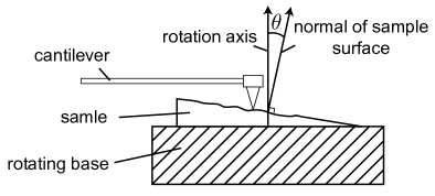
Figure 1: Schematic illustration of the tilt problem occurring in the rotational scanning.

Mathematically the control problem can be formulated as follows. Let us denote the height measured from the tip as $x(t)$. $x(t)$ is governed by a simple first order differential equation

$$\dot{x}(t)=-\gamma x(t)+f(\omega t)+u(t),$$ (1)

where $\gamma>0$ is a stiffness of the cantilever, $\omega$ is a rotation angular velocity, $f(\omega t+T)=f(\omega t)=\sum_{i=0}^{+\infty}f_{i}\sin(i\omega t+\varphi_{i})$ is a $T$-periodic force containing the information on the topography of the surface and the tilting angle, and $u(t)$ represents the control force appears due to the up-and-down lifting mechanism. The parameter $\gamma$ assumed to be much larger than $\omega$. In fact, in the experiment Ulcinas2017 $\omega$ is set to approximately 50 Hz while $\gamma$ is of the order of kHz, thus $\omega/\gamma<1$ is justifiable. Note that in Eq. (1) we omitted any factor next to the term $u(t)$ meaning that the external force comes with sensitivity factor equal to one. It motivated by the fact that the variable $x(t)$ can always be re-scaled in such a way that Eq. (1) is well justified.

For the control-free case ($u(t)=0$) solution of Eq. (1) can be written as a power series expansion of the ratio $\omega/\gamma$:

$$x(t)=x_{0}(t)+x_{1}(t)+\mathcal{O}\left((\omega/\gamma)^{2}\right).$$ (2)

Substitution of the last expression to Eq. (1) yields $x_{0}(t)=0$ and $x_{1}(t)=f(\omega t)/\gamma$ meaning that $x(t)\approx f(\omega t)/\gamma$ and thus resembles a shape of the roughness of the surface. Restriction to the zero and the first order terms in expansion (2) is equivalent to a simplification of Eq. (1) up to an equation

$$0=-\gamma x(t)+f(\omega t)+u(t).$$ (3)

Further in the paper in all analytical derivation we will always use simplified Eq. (3) instead of full Eq. (1), except in numerical calculations just to show that the controller developed for (3) in fact works well for the systems (1) if the condition $\omega/\gamma<1$ holds.

Our goal is to construct linear time-invariant controller accepting as an input the delayed signal $x(t-\tau)$ and producing the output $u(t)$ such that Eq. (3) yields the solution

$$x(t)=\frac{f_{0}}{\gamma}+\sum_{i=2}^{+\infty}\frac{f_{i}}{\gamma}\sin(i\omega t+\varphi_{i}),$$ (4)

i.e. $x(t)$ reproduces the roughness of the surface without the first Fourier harmonic. The time delay $\tau$ assumed to be unknown, jet not larger than the period $T=2\pi/\omega$, so that $\tau/T<1$.

3 Construction of the controller

As a main idea of our control algorithm we will use the controller developed in Ref. Olyaei2015 ; AzimiOlyaei2018 . The controller contains a system of harmonic oscillators coupled with the input signal and used to stabilize an unknown unstable periodic orbit in a dynamical system. Here our goal is different: instead of stabilization we want the elimination of the first Fourier harmonic. Thus we will modify the controller Olyaei2015 ; AzimiOlyaei2018 to fulfill out goal.

3.1 Restriction to the case of one harmonic in the force $f(\omega t)$

Firstly, one can solve a simplified task. In particular, let us say that the force $f(\omega t)$ contains only the first harmonic, i.e. we have $f(\omega t)=f_{1}\sin(\omega t)$. Here and further in text, without loss of generality, we set the initial phase $\varphi_{1}=0$. For such a case one can use only one harmonic oscillator coupled with the delayed system output $x(t-\tau)$:

$$\dot{a}_{1}(t) =-\omega b_{1}(t)+\alpha_{1}x(t-\tau),$$ (5a)

$$\dot{b}_{1}(t) =\omega a_{1}(t)+\beta_{1}x(t-\tau).$$ (5b)

Here $a_{1}(t)$ and $b_{1}(t)$ are the real-valued dynamical variables of the harmonic oscillator, $\alpha_{1}$ and $\beta_{1}$ are the coupling constants. The output of the controller

$$u(t)=Ka_{1}(t),$$ (6)

where $K$ stands for the control gain. The closed loop system (3), (5) and (6) possesses our desired solution

$$x(t) =0,$$ (7a)

$$a_{1}(t) =-\frac{f_{1}}{K}\sin(\omega t),$$ (7b)

$$b_{1}(t) =\frac{f_{1}}{K}\cos(\omega t).$$ (7c)

Small deviations $\delta x(t)$, $\delta a_{1}(t)$ and $\delta b_{1}(t)$ from the desired solution (7) satisfy following linear time-invariant system of equations

$$\delta x(t) =\frac{K}{\gamma}\delta a_{1}(t),$$ (8a)

$$\delta\dot{a}_{1}(t) =-\omega\delta b_{1}(t)+\alpha_{1}\delta x(t-\tau),$$ (8b)

$$\delta\dot{b}_{1}(t) =\omega\delta a_{1}(t)+\beta_{1}\delta x(t-\tau).$$ (8c)

By using the Laplace transform and the formalism of transfer function one can formulate the stability of the closed loop system (8). We will use standard uppercase letter notation for the Laplace transformed signals. In particular, if we have a signal $y(t)$ in the time domain, then the Laplace transformed signal in the frequency domain denoted as $Y(s)=\mathcal{L}(y)=\int_{0}^{+\infty}y(t)\exp(-st)\mathrm{d}t$.

Simple Eq. (8a) defines dynamics of a plant (system to be controlled). The plant as an input signal accepts $\delta u(t)=K\delta a_{1}(t)$ and produce an output signal $\delta x(t-\tau)$ which is delayed plant variable $\delta x(t)$. Thus the plant transfer function

$$P(s)=\frac{\delta X(s)\mathrm{e}^{-\tau s}}{\delta U(s)}=\frac{\delta X(s)\mathrm{e}^{-\tau s}}{K\delta A_{1}(s)}=\frac{\mathrm{e}^{-\tau s}}{\gamma}.$$ (9)

The controller described by Eqs. (8b), (8c) accepts $\delta x(t-\tau)$ as an input signal and produce $\delta u(t)=K\delta a_{1}(t)$ as an output signal. The transfer function of the controller is

$$C(s)=K\frac{\delta A_{1}(s)}{\delta X(s)\mathrm{e}^{-\tau s}}=K\frac{s\alpha_{1}-\omega\beta_{1}}{s^{2}+\omega^{2}}.$$ (10)

It is important to mention that the controller of full variables (5) and the controller for small deviations (8b), (8c) coincides: both systems are linear time-invariant thus has the same transfer function, meaning that the same Eq. (10) would be derived for the controller’s (5) transfer function $C(s)=KA_{1}(s)/[X(s)\mathrm{e}^{-\tau s}]$. In contrast, the plant of full variables (3) is not time-invariant due to the term $f(\omega t)$. Therefore we derived Eq. (8a) which is time-invariant.

By having the plant transfer function (9) and the controller transfer function (10) one can write the transfer function of the whole closed-loop system (8)

$$G(s)= \frac{C(s)P(s)}{1-C(s)P(s)}$$ (11)

$$= K\frac{s\alpha_{1}-\omega\beta_{1}}{\gamma\mathrm{e}^{\tau s}\left(s^{2}+\omega^{2}\right)-K\left(s\alpha_{1}-\omega\beta_{1}\right)}.$$

The stability of the system (11) is determined by the real parts of poles, namely the system is stable if and only if all poles have negative real parts. Let us analyze only positive $K$ values, since from Eq. (10) one can see that the negative $K$ reproduces the same $C(s)$ if we flip the signs for both parameters $\alpha_{1}$ and $\beta_{1}$. The equation for the poles is

$$\mathrm{e}^{\tau s}\left(s^{2}+\omega^{2}\right)-\frac{K}{\gamma}\left(s\alpha_{1}-\omega\beta_{1}\right)=0.$$ (12)

In the case $\tau=0$ one has only two poles. By using the Vieta’s formulas it is easy to derive necessary and sufficient stability conditions

$$\alpha_{1}<0\quad\mathrm{and}\quad\frac{K}{\gamma}\beta_{1}>-\omega.$$ (13)

For non-zero delay Eq. (12) provides an infinite number of poles whose are difficult to manage analytically. Therefore we analyze Eq. (12) numerically and depicted the stability region in Fig. 2 for several values of $\tau/T$. When the delay time is increased the horizontal stability border ($\beta_{1}=-\frac{\gamma}{K}\omega$) remains unchanged (thick horizontal line in Fig. 2). It can be seen from Eq. (12) when we substitute the root $s=0$ and obtain the stability border $\beta_{1}=-\frac{\gamma}{K}\omega$. In contrast, the vertical stability border ($\alpha_{1}=0$) depends on $\tau/T$ and it modifies to a parabola-type curve (see Fig. 2).

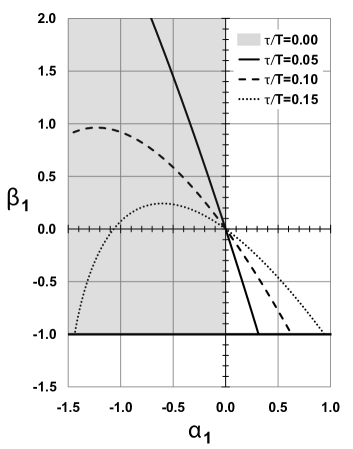
Figure 2: The closed-loop systems (11) stability region calculated numerically from Eq. (12) with different values of the ratio $\tau/T$. The parameters are set to $K/\gamma=1$ and $\omega=1$.

In order to demonstrate successful work of our controller, in Fig. 3 we depicted numerical simulation of the plant equation (1) with $f(\omega t)=f_{1}\sin(\omega t)$ and feedback loop defined by Eqs. (5) and (6). As one can see, the controller achieves stabilization for non-zero delay $\tau/T=0.15$. Yet further increase of the time delay leads to loose of the stability.

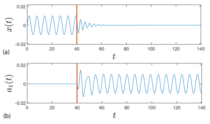
Figure 3: The results of the numerical simulation of closed-loop system (1), (5) and (6). Before time moment $t=40$ the system is in control-free regime ($K=0$). (a) – the dynamics of the plant variable, (b) – the same for the first controller variable $a_{1}(t)$. The parameters are following: $K/\gamma=1$, $\gamma=200$, $f_{1}=1$, $\omega=1$, $\alpha_{1}=-1$, $\beta_{1}=-0.5$ and the time delay $\tau/T=0.15$.

3.2 The case of full set of harmonics

This time we assume that the force $f(\omega t)$ contains a set of $N$ Fourier harmonics

$$f(\omega t)=\sum_{i=0}^{N}f_{i}\sin\left(i\omega t+\varphi_{i}\right).$$ (14)

In particular, $N$ can be equal to $+\infty$ meaning that all harmonics contribute to the force $f$. Similarly to Subsec. 3.1 without loss of generality we can assume that $\varphi_{1}=0$. Since we have $N$ Fourier harmonics, our controller should contain set of $N$ harmonic oscillators coupled to the input signal $x(t-\tau)$. For such a case, Eqs. (5) can be generalized as follows:

$$\dot{a}_{0}(t) =\alpha_{0}\left[x(t-\tau)-\sum_{i=0\atop i\neq 1}^{N}a_{i}(t)\right],$$ (15a)

$$\dot{a}_{j}(t) =-j\omega b_{j}(t)+\alpha_{j}\left[x(t-\tau)-\sum_{i=0\atop i\neq 1}^{N}a_{i}(t)\right],$$ (15b)

$$\dot{b}_{j}(t) =j\omega a_{j}(t)+\beta_{j}\left[x(t-\tau)-\sum_{i=0\atop i\neq 1}^{N}a_{i}(t)\right],$$ (15c)

where $j=1,2,\ldots,N$. Here $\alpha_{j}$ and $\beta_{j}$ are coupling constants to be determined below. The output of the controller has the same form (6) as in the one harmonic case.

The closed loop system (3), (15) and (6) possesses the solution of $x(t)$ without the first harmonic

$$x(t) =\frac{1}{\gamma}\sum_{i=0\atop i\neq 1}^{N}f_{i}\sin\left(i\omega t+\varphi_{i}\right),$$ (16a)

$$a_{0}(t) =\frac{f_{0}}{\gamma},$$ (16b)

$$a_{1}(t) =-\frac{f_{1}}{K}\sin(\omega t),$$ (16c)

$$b_{1}(t) =\frac{f_{1}}{K}\cos(\omega t),$$ (16d)

$$a_{j}(t) =\frac{f_{j}}{\gamma}\sin\left(j\omega(t-\tau)+\varphi_{j}\right),$$ (16e)

$$b_{j}(t) =-\frac{f_{j}}{\gamma}\cos\left(j\omega(t-\tau)+\varphi_{j}\right),$$ (16f)

with $j=2,3,\ldots,N$. While the controller equations (15) is the linear time-invariant system, the plant (3) is linear but not time-invariant system. In order to threat the system using transfer function formalism, one should have the linear time-invariant system. Therefore one can write the equations for the small deviation from the target solution (16):

$$\delta x(t) =\frac{K}{\gamma}\delta a_{1}(t),$$ (17a)

$$\delta\dot{a}_{0}(t) =\alpha_{0}\left[\delta x(t-\tau)-\sum_{i=0\atop i\neq 1}^{N}\delta a_{i}(t)\right],$$ (17b)

$$\delta\dot{a}_{j}(t) =-j\omega\delta b_{j}(t)+\alpha_{j}\left[\delta x(t-\tau)-\sum_{i=0\atop i\neq 1}^{N}\delta a_{i}(t)\right],$$ (17c)

$$\delta\dot{b}_{j}(t) =j\omega\delta a_{j}(t)+\beta_{j}\left[\delta x(t-\tau)-\sum_{i=0\atop i\neq 1}^{N}\delta a_{i}(t)\right],$$ (17d)

with $j=1,2,\ldots,N$. The transfer function of the plant system (17a) has the same simple form (9) as in the previous subsection 3.1. Yet the controller’s transfer function $C(s)=\delta U(s)/[\delta X(s)\mathrm{e}^{-\tau s}]$ is much more complicated. In Appendix A we provide derivation of the controller’s transfer function:

$$C(s)= K\left(\alpha_{1}s-\beta_{1}\omega\right)s\prod_{j=2}^{N}\left(s^{2}+j^{2}\omega^{2}\right)$$ (18)

$$\times\left\{(s+\alpha_{0})\prod_{j=1}^{N}\left(s^{2}+j^{2}\omega^{2}\right)\right.$$

$$\left.+s\sum_{k=2}^{N}\left(\alpha_{k}s-k\beta_{k}\omega\right)\prod_{j=1\atop j\neq k}^{N}\left(s^{2}+j^{2}\omega^{2}\right)\right\}^{-1}.$$

The zeros of the transfer function are $s=0$, $s=\beta_{1}\omega/\alpha_{1}$, $s=\pm\mathrm{i}k\omega$ for $k=2,3,\ldots,N$, while the poles are determined by the expression in the curly brackets. The closed-loop system transfer function $G(s)$ can be obtained by the same formula (11). The stability of the solution (16) is determined by the poles of the function $G(s)$ involving both the zeros and the poles of the controller’s transfer function $C(s)$. To be more precise, the poles of $G(s)$ are solutions for the equation

$$\gamma(s+\alpha_{0})\prod_{j=1}^{N}\left(s^{2}+j^{2}\omega^{2}\right)$$ (19)

$$+ \gamma s\sum_{k=2}^{N}\left(\alpha_{k}s-k\beta_{k}\omega\right)\prod_{j=1\atop j\neq k}^{N}\left(s^{2}+j^{2}\omega^{2}\right)$$

$$- K\mathrm{e}^{-\tau s}s\left(\alpha_{1}s-\beta_{1}\omega\right)\prod_{j=2}^{N}\left(s^{2}+j^{2}\omega^{2}\right)=0.$$

Such equation has many parameters. In order to simplify it, we set some particular form of the coupling constants $\alpha_{k}$ and $\beta_{k}$:

$$\alpha_{0}=\alpha,\;\alpha_{1}=-2\alpha\frac{\gamma}{K},\;\beta_{1}=2\beta\frac{\gamma}{K},$$ (20)

$$\alpha_{k}=2\alpha,\;\beta_{k}=-2\beta/k\quad\mathrm{for}\;k=2\ldots N.$$

Thus we have only two real index-less variables $\alpha$ and $\beta$. The motivation behind such form is that it significantly simplifies stability analysis. Now Eq. (19) reduces to

$$(s+\alpha)\prod_{j=1}^{N}\left(s^{2}+j^{2}\omega^{2}\right)$$ (21)

$$+ 2s\left(\alpha s+\beta\omega\right)\sum_{k=1}^{N}\mathrm{e}^{-\tau s\delta_{1,k}}\prod_{j=1\atop j\neq k}^{N}\left(s^{2}+j^{2}\omega^{2}\right)=0,$$

where $\delta_{1,k}$ is non-zero only for $k=1$. Similar to Eq. (12), in order to analytically find the poles of the closed-loop transfer function $G(s)$ we consider the simplest case $\tau=0$. Now Eq. (21) reads

$$(s+\alpha)q(s)+\left(\alpha s+\beta\omega\right)\frac{\mathrm{d}q(s)}{\mathrm{d}s}=0,$$ (22)

where the function $q(s)$ is defined as

$$q(s)=\prod_{j=1}^{N}\left(s^{2}+j^{2}\omega^{2}\right).$$ (23)

In Appendix B we showed that in the limit $N\rightarrow+\infty$ the necessary and sufficient condition for the roots of Eq. (22) to have negative real parts is

$$\alpha>0\quad\mathrm{and}\quad\frac{\beta}{\omega}>-\frac{1}{4}.$$ (24)

In contrast to the previous stability condition (13), here the stability border goes along $\beta/\omega=-1/4$ while in the one harmonic case (13) it goes along $\beta/\omega=-1/2$ (note that the relation of the index-less coupling constants $\alpha$ and $\beta$ with $\alpha_{1}$ and $\beta_{1}$ is defined by Eq. (20)).

For the non-zero time delay we numerically calculated the stability region. We analyzed Eq. (21) in the limit $N\rightarrow+\infty$ and calculated events when the pair (or several pairs) of complex conjugate roots crossed imaginary axis, denoting loose of the stability. In Fig. 4 we plot borders of the stability regions for several values of the ratio $\tau/T$. As one can see the stability region significantly shrinks once we increase the time-delay. Yet we point out that there are “universal” values $(\alpha/\omega,\beta/\omega)=(0.1,-0.1)$ where the system remains stable at least up to $\tau/T=0.15$ making them as a good starting point in a real experimental situation.

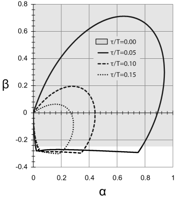
Figure 4: The stability regions for the roots of Eq. (21) calculated numerically in the limit $N\rightarrow+\infty$. The frequency $\omega$ set to be equal to 1.

In order to demonstrate successful application of the controller, we numerically integrate the plant (1) with the external force $f(\omega t)$ defined by Eq. (14) and the controller defined by Eqs. (15), (6). In Fig. 5 (a) we plotted the plant variable $x(t)$ and compared it with the external force without the first Fourier harmonic $[f(\omega t)-f_{1}\sin(\omega t)]/\gamma$. In the case of successful first harmonic elimination, according to Eq. (16a), the plant variable should settle to the filtered external force. This is exactly what we observe in Fig. 5 (a) after $t=40$ and transient time. The time delay is set to $\tau/T=0.15$. Further increase of the time delay will lead to destabilization of the closed-loop system.

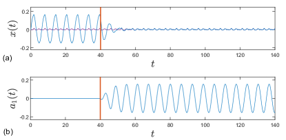
Figure 5: The results of the numerical simulation of closed-loop system (1), (14), (15) and (6) with the finite number of the harmonics, $N=10$. Before time moment $t=40$ the system is in control-free regime ($K=0$). (a) – the dynamics of the plant variable (blue curve) and the external force without the first harmonic $f_{0}/\gamma+\sum_{i=2}^{N}f_{i}/\gamma\sin(i\omega t+\varphi_{i})$ (purple line), (b) – the same for the first controller variable $a_{1}(t)$. The parameters are following: $K/\gamma=1$, $\gamma=100$, $\omega=1$, $\alpha=0.1$, $\beta=-0.1$, $\tau/T=0.15$, the amplitudes $f_{i}$ and the phases $\varphi_{i}$ generated randomly except $f_{1}$ which is artificially increased in order to better express successful work of the controller. The phases $\varphi_{i}$ generated from uniform distribution of the interval $[0,2\pi]$, while the amplitudes $f_{i}$ are generated from uniform distribution of the interval $[0,1]$ and additionally divided by the harmonic number $i$.

4 The block scheme of the controller

The controller described by Eqs. (15) is linear time-invariant controller with the transfer function (18). Taking in to account the form of coupling constants (20) we obtain the transfer function

$$C(s)= (-\gamma)2\left(\frac{\alpha s+\beta\omega}{s^{2}+\omega^{2}}\right)$$ (25)

$$\times\left\{1+\frac{\alpha}{s}+2\sum_{j=2}^{N}\frac{\alpha s+\beta\omega}{s^{2}+j^{2}\omega^{2}}\right\}^{-1}.$$

Such transfer function can be represented by the block scheme depicted in Fig. 6, where

$$H_{j}(s)=2\frac{\alpha s+\beta\omega}{s^{2}+j^{2}\omega^{2}}$$ (26)

for $j=1,2,\ldots,N$ and

$$H_{0}(s)=\frac{\alpha}{s}$$ (27)

are the transfer functions of the harmonic oscillators. The logical description of the block scheme can be following. On the first stage we remove from the input $x(t-\tau)$ all non-first harmonics, thus producing the signal $y(t)$ containing only the first harmonic. The signal $y(t)$ is exactly the term in square brackets of Eq. (15). Then $y(t)$ is coupled with all oscillators. The oscillators $H_{0}(s)$ and $H_{2,3,\ldots,N}(s)$ trying to adjust their amplitudes and phases in such a way that $y(t)$ should contain only the first harmonic. If so happens then $y(t)$ coupled with $H_{1}(s)$ produces the oscillator’s output $a_{1}(t)$ which is gained by the factor $-\gamma$ and fed to the plant. If $H_{1}(s)$ has well adjusted amplitude and phase such that $-\gamma a_{1}(t)$ eliminates the first harmonic from the plant’s output $x(t)$ then $y(t)=0$ and all oscillators are no longer disturbed by $y(t)$. In such a way $x(t)$ no longer possesses the first harmonic.

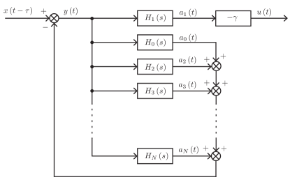
Figure 6: The block scheme representing the controller (25) containing the set of the harmonic oscillators $H_{j}(s)$.

5 Controller’s equation for the infinite number of the harmonics

The harmonic oscillator method Olyaei2015 with a particular choice of the coupling constants ($\alpha_{j}=\alpha$ and $\beta_{j}=0$) and in the limit $N\rightarrow+\infty$ is equivalent to a extended delayed feedback control scheme PyrHarmOsc2015 . Taking the limit when the number of harmonic oscillators goes to infinity one can simplify our transfer function (25) and using inverse Laplace transform obtain controller scheme in the time domain. Instead of having an infinite number of ordinary differential equations, as in Eqs. (15), such scheme can be written as a system of a neutral-type delay differential equations. Thus the number of the dynamical variables remains finite, yet the infinite dimension is encoded via delayed terms.

Using notation (23), the transfer function reads

$$C(s)= -2\gamma\left(\alpha s+\beta\omega\right)sq(s)$$ (28)

$$\times\left\{(s+\alpha)\left(s^{2}+\omega^{2}\right)q(s)-2\left(\alpha s+\beta\omega\right)sq(s)\right.$$

$$+\left.\left(s^{2}+\omega^{2}\right)\left(\alpha s+\beta\omega\right)\frac{\mathrm{d}q(s)}{\mathrm{d}s}\right\}^{-1}.$$

In the limit $N\rightarrow+\infty$ the function $q(s)$ can be written as a hyperbolic sine (44), therefore the last expression reads (we divided the numerator and the denominator by the factor $\sinh\left(\pi s/\omega\right)$)

$$C(s)=-2\gamma\left(\alpha s^{3}+\beta\omega s^{2}\right)$$ (29)

$$\times\left\{\left(s^{4}-\alpha s^{3}+\omega(\omega-2\beta)s^{2}+\alpha\omega^{2}s\right)\right.$$

$$+\left.\left(\alpha s^{3}+\beta\omega s^{2}+\alpha\omega^{2}s+\omega^{3}\beta\right)\left[\frac{\pi s}{\omega}\coth\left(\frac{\pi s}{\omega}\right)-1\right]\right\}^{-1}.$$

Since the hyperbolic cotangent can be written as

$$\coth\left(\frac{\pi s}{\omega}\right)=\frac{1+\mathrm{e}^{-Ts}}{1-\mathrm{e}^{-Ts}},$$ (30)

we end up with the following expression

$$C(s)=-2\gamma\left(\alpha s^{3}+\beta\omega s^{2}\right)\left[1-\mathrm{e}^{-Ts}\right]$$ (31)

$$\times\left\{s^{4}\left(1+\frac{\alpha\pi}{\omega}\right)\left[1-\frac{\omega-\alpha\pi}{\omega+\alpha\pi}\mathrm{e}^{-Ts}\right]\right.$$

$$+s^{3}(\beta\pi-2\alpha)\left[1-\frac{2\alpha+\beta\pi}{2\alpha-\beta\pi}\mathrm{e}^{-Ts}\right]$$

$$+s^{2}\omega(\omega-3\beta+\alpha\pi)\left[1-\frac{\omega-3\beta-\alpha\pi}{\omega-3\beta+\alpha\pi}\mathrm{e}^{-Ts}\right]$$

$$+\left.s\beta\pi\omega^{2}\left[1+\mathrm{e}^{-Ts}\right]-\beta\omega^{3}\left[1-\mathrm{e}^{-Ts}\right]\right\}^{-1}.$$

The inverse Laplace transformation of the last expression is rather tedious and technical work, thus we moved it to Appendix C. As a result we obtain neutral-type delay differential equations consisting of 4 first order differential equations

$$\dot{q}_{0}(t) =q_{1}(t)+f_{0}(t),$$ (32a)

$$\dot{q}_{1}(t) =q_{2}(t)+f_{1}(t),$$ (32b)

$$\dot{q}_{2}(t) =q_{3}(t)+f_{2}(t),$$ (32c)

$$\dot{q}_{3}(t) =q_{4}(t)+f_{3}(t),$$ (32d)

5 difference equations with delayed terms

$$f_{0}(t)= R_{4}f_{0}(t-T)$$

$$+N_{1}\left[x(t-\tau)-x(t-\tau-T)\right],$$ (33a)

$$f_{1}(t)= R_{4}f_{1}(t-T)$$

$$+N_{2}\left[x(t-\tau)-x(t-\tau-T)\right]$$

$$+M_{3}\left[f_{0}(t)-R_{3}f_{0}(t-T)\right],$$ (33b)

$$f_{2}(t)= R_{4}f_{2}(t-T)$$

$$+M_{3}\left[f_{1}(t)-R_{3}f_{1}(t-T)\right]$$

$$+M_{2}\left[f_{0}(t)-R_{2}f_{0}(t-T)\right],$$ (33c)

$$f_{3}(t)= R_{4}f_{3}(t-T)$$

$$+M_{3}\left[f_{2}(t)-R_{3}f_{2}(t-T)\right]$$

$$+M_{2}\left[f_{1}(t)-R_{2}f_{1}(t-T)\right]$$

$$-M_{1}\left[f_{0}(t)+f_{0}(t-T)\right],$$ (33d)

$$q_{4}(t)= R_{4}q_{4}(t-T)+M_{3}\left[q_{3}(t)-R_{3}q_{3}(t-T)\right]$$

$$+M_{2}\left[q_{2}(t)-R_{2}q_{2}(t-T)\right]$$

$$-M_{1}\left[q_{1}(t)+q_{1}(t-T)\right]$$

$$+M_{0}\left[q_{0}(t)-q_{0}(t-T)\right],$$ (33e)

and the set of parameters $R_{2}=\frac{\omega-3\beta-\alpha\pi}{\omega-3\beta+\alpha\pi}$, $R_{3}=\frac{2\alpha+\beta\pi}{2\alpha-\beta\pi}$, $R_{4}=\frac{\omega-\alpha\pi}{\omega+\alpha\pi}$, $N_{1}=\frac{2\alpha\omega}{\omega+\alpha\pi}$, $N_{2}=\frac{2\beta\omega^{2}}{\omega+\alpha\pi}$, $M_{0}=\frac{\beta\omega^{4}}{\omega+\alpha\pi}$, $M_{1}=\frac{\beta\pi\omega^{3}}{\omega+\alpha\pi}$, $M_{2}=\frac{\omega^{2}(3\beta-\alpha\pi-\omega)}{\omega+\alpha\pi}$ and $M_{3}=\frac{\omega(2\alpha-\beta\pi)}{\omega+\alpha\pi}$. The controller’s output is defined as $u(t)=-\gamma q_{0}(t)$. Since the controller as the input signal receives the delayed plant’s output $x(t-\tau)$, the term $x(t-\tau-T)$ is the same delayed plant’s output but additionally delayed by the period $T$. The controller (32), (33) produce absolutely the same output $u(t)$ as the controller (15) for $N\rightarrow+\infty$ if both initial conditions are matched. Typical initial conditions for Eqs. (15) is when all dynamical variables are set to zero: $a_{j}(0)=0$, $b_{j}(0)=0$. It corresponds a zero initial conditions for (32), (33) when all dynamical variables $q_{i}$ and $f_{i}$ and their delay lines are set to zero. Important thing is that the delay line for $x(t-\tau)$ is also should be set to zero, meaning that the term $x(t-\tau-T)$ actually should be calculated as $x(t-\tau-T)\sigma(t-T)$ where $\sigma(t)$ stands for a heaviside step function.

While it might looks like the controller (32), (33) is superior to the truncated version (15) since it deals with all harmonics, that is not exactly true. The involvement of all harmonics is an advantage and a disadvantage at the same time. In typical experiment the signal $x(t-\tau)$ is measured not continuously but at the discrete time moments with fixed time step. It means that Eqs. (32), (33) also should be integrated using a fixed time step integration scheme. Since the controller (32), (33) effectively contains all harmonics, the fixed time step integration scheme applied to (32), (33) should deal with extremely high harmonic numbers. But it means that we have a situation when the period of the harmonic oscillator (with extremely high harmonic number) is much lower than the integration step. Thus it leads to an inaccuracy of the integration scheme. However, such inaccuracy is not visible on a short time interval, and only on a long time interval the error accumulates and gives an unstable dynamics of the controller. In contrast, the truncated controller (15) does not have such an issue.

In order to compare the truncated controller with the controller described by the neutral-type delay differential equations we performed following computation: the plant equation (1) is integrated using high-precision adaptive time step method $\mathtt{ode45}$ (standard MatLab integrator) while the controller Eqs. (15) or Eqs. (32), (33) is integrated using the fixed time step Adams-Bashforth 3th order method. In Fig. 7 we depicted the successful work of both controllers on a different time scales. Fig. 7(a) shows transient dynamics when controllers are turned-on. Both dynamics almost coincide. Fig. 7(b) shows the dynamics after some time of working controllers. Again both dynamics almost coincide. In contrast, Fig. 7(c) depicts the dynamics after long time of working controllers. Here one can see that accumulated error gives increasing amplitude for the controller (32), (33) while the truncated controller remains stable.

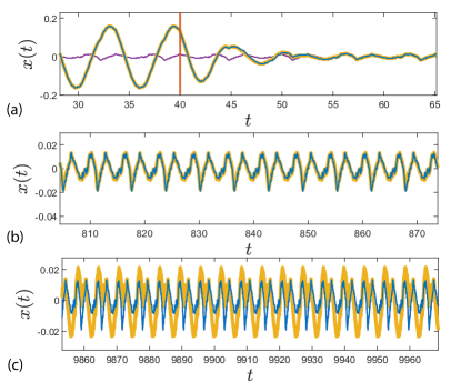
Figure 7: The comparison of both controllers: the controller (32), (33) and truncated controller (15). Similar to Fig. 5, blue line represents truncated controller and purple line is the external force without the first harmonic (desirable output). Yet, here we have thick yellow line representing the controller (32), (33). The parameters are the same as in Fig. 5 except now the external force has 80 harmonics and the truncated controller has only 5 harmonics. One can see that in (a) and (b) the blue line coincide with the thick yellow line, but after long time interval in (c) the yellow line alternates from the desirable output.

6 Discussion and conclusions

We study the situation where the plant produces periodic output signal and there is a delay line between the plant and the controller. The delay time assumed to be unknown. We developed control algorithm to eliminate the first harmonic in the plant’s output without disturbing all other harmonics in the periodic signal. The algorithm is based on a modified version of system of harmonic oscillators Olyaei2015 ; AzimiOlyaei2018 used to stabilize an unstable periodic orbit with an unknown profile. The demand of such algorithm naturally appears in the experiments of the rotational scanning atomic force microscopy Ulcinas2017 .

Our controller is a linear time invariant system described by the transfer function (25). Such transfer function has three undefined constants: coupling constants $\alpha$ and $\beta$, and the gain factor $\gamma$. We calculated the stability of the controller (see Fig. 4) for different time delays and observed that a good choice of the coupling constants is $\alpha=0.1$, $\beta=-0.1$. The factor $\gamma$ is not exactly controller’s gain $K$ appeared in the controller’s realization in time domain, Eqs. (15). Since we used particular choice of the coupling constants (20), an interchange of $K$ to $\gamma$ happened. It means that in the practical realization we should guess the value $\gamma$ and set $K=\gamma$. The parameter $\gamma$ has well defined physical interpretation: the relaxation time of the plant variable, or a stiffness of a cantilever in the case of atomic force microscopy. Thus some information on $\gamma$ can be known a priori. Yet not accurate guess of $\gamma$, in the worst case scenario, can only lead to instability. But it does not change the purpose of the controller: to eliminate the first harmonic.

The controller can be extended in different directions. For example one can ask whether it is possible to eliminate not only the first harmonic, but a some set of prescribed harmonics. Intuitively, the more harmonics we want to eliminate the more unstable controller becomes. Yet it is unexplored possibility requiring further work. Another potentially interesting question is how can we deal with higher delay time. Since the plant transfer function (9) is extremely simple, a classical Smith’s predictor Smith57 should fit well this task. Yet it requires additional researches which can be done in further works.

Appendix A Derivation of the controller transfer function

Here we will derive the transfer function for the controller (15) and (6) defined as a ratio of the form $C(s)=\allowbreak U(s)/[X(s)\mathrm{e}^{-\tau s}]\allowbreak=KA_{1}(s)/[X(s)\mathrm{e}^{-\tau s}]$. The same transfer function would be obtained if we will use Eqs (17b), (17c), (17d) and the definition of the transfer function $C(s)=K\delta A_{1}(s)/[\delta X(s)\mathrm{e}^{-\tau s}]$.

First let us introduce complex-valued dynamical variables $\tilde{a}_{j}(t)$ defined as $\tilde{a}_{j}(t)=[a_{j}(t)+\mathrm{i}b_{j}(t)]/2$ for $j=1,2,\ldots,N$, $\tilde{a}_{j}(t)=[a_{-j}(t)-\mathrm{i}b_{-j}(t)]/2$ for $j=-1,-2,\ldots,-N$ and $\tilde{a}_{0}(t)=a_{0}(t)$. The differential equations for them have more symmetry. In fact the original paper on method of the harmonic oscillators Olyaei2015 operates in this setup. Hence, Eqs. (15) read

$$\dot{\tilde{a}}_{j}(t)=\mathrm{i}j\omega\tilde{a}_{j}(t)+\kappa_{j}\left[x(t-\tau)-\sum_{i=-N\atop|i|\neq 1}^{N}\tilde{a}_{i}(t)\right],$$ (34)

where $j=-N,-N+1,\ldots,N$. Here we introduced new coupling constants $\kappa_{j}=[\alpha_{j}+\mathrm{i}\beta_{j}]/2$ for positive $j$, $\kappa_{j}=[\alpha_{-j}-\mathrm{i}\beta_{-j}]/2$ for negative $j$, and $\kappa_{0}=\alpha_{0}$. Therefore we have $\tilde{a}_{j}^{*}(t)=\tilde{a}_{-j}(t)$ and $\kappa_{j}^{*}=\kappa_{-j}$ meaning that the complex conjugation is equivalent to the sign flipping of the index.

Next step is to apply the Laplace transformation for the system of differential equations (34). By introducing the column vector $\tilde{\mathbf{A}}(s)=(\tilde{A}_{-N}(s),\tilde{A}_{-N+1}(s),\ldots,\tilde{A}_{N}(s))^{T}$ (here ^T denotes transposition) containing the Laplace transformations for all dynamical variables $\tilde{a}_{j}(t)$, one can write (34) as

$$\mathbf{M}\tilde{\mathbf{A}}(s)=\mathrm{e}^{-\tau s}X(s)\left(\begin{array}[]{c}\kappa_{-N}\\ \kappa_{-N+1}\\ \vdots\\ \kappa_{N}\end{array}\right).$$ (35)

The matrix $\mathbf{M}$ has following form

$$\mathbf{M}= \mathrm{diag}\left[s-\mathrm{i}(-N)\omega,s-\mathrm{i}(-N+1)\omega,\ldots,s-\mathrm{i}N\omega\right]$$ (36)

$$+\left(\begin{array}[]{c}\kappa_{-N}\\ \kappa_{-N+1}\\ \vdots\\ \kappa_{N}\end{array}\right)\left(\begin{array}[]{ccccccccc}1&\ldots&1&0&1&0&1&\ldots&1\end{array}\right),$$

where $\mathrm{diag}[c_{1},c_{2},\ldots]$ denotes a diagonal matrix with the elements $c_{1}$, $c_{2}$, $\ldots$ on the diagonal. The matrix $\mathbf{M}$ has special structure: it is written as a sum of diagonal matrix and the outer product matrix. Moreover, one of the vectors in the construction of the outer product matrix has only ones and zeros. Because of such special form one can easy find an inverse matrix. Using notation $p_{j}(s)=1/(s-\mathrm{i}j\omega)$ one can read

$$\mathbf{M}^{-1} =\mathrm{diag}\left[p_{-N},p_{-N+1},\ldots,p_{N}\right]-\left[1+\sum_{j=-N\atop|j|\neq 1}^{N}\kappa_{j}p_{j}\right]^{-1}$$ (37)

$$\times\left(\begin{array}[]{c}\kappa_{-N}p_{-N}\\ \kappa_{-N+1}p_{-N+1}\\ \vdots\\ \kappa_{N}p_{N}\end{array}\right)\left(\begin{array}[]{ccccccccc}p_{-N}&\ldots&p_{-2}&0&p_{0}&0&p_{2}&\ldots&p_{N}\end{array}\right).$$

By combining Eqs. (37) and (35) we finally obtain the Laplace transform of the output signal

$$U(s)= K\left(\tilde{A}_{-1}(s)+\tilde{A}_{1}(s)\right)$$ (38)

$$= K\mathrm{e}^{-\tau s}X(s)\left[1+\sum_{j=-N\atop|j|\neq 1}^{N}\frac{\kappa_{j}}{s-\mathrm{i}j\omega}\right]^{-1}\left(\frac{\kappa_{-1}}{s+\mathrm{i}\omega}+\frac{\kappa_{1}}{s-\mathrm{i}\omega}\right).$$

Subsequently the transfer function

$$C(s)=K\left[1+\frac{\alpha_{0}}{s}+\sum_{j=2}^{N}\frac{\alpha_{j}s-j\beta_{j}\omega}{s^{2}+j^{2}\omega^{2}}\right]^{-1}\left(\frac{\alpha_{1}s-\beta_{1}\omega}{s^{2}+\omega^{2}}\right).$$ (39)

Appendix B Stability condition for the closed-loop system

The polynomial (22) is the $(2N+1)$-order polynomial with real coefficients. The necessary condition for the stability is that all coefficients should be positive. The coefficient next to the term $s^{2N}$ is $\alpha(2N+1)$. Thus the necessary stability condition is

$$\alpha>0.$$ (40)

When $\alpha$ is positive, the only way to loose (or gain) the stability is the case when the pair (or several pairs) of complex conjugate roots cross the imaginary line $\Re(s)=0$, because $s=0$ can not be a solution of Eq. (22) for $\alpha\neq 0$.

Next, let us look for the coefficient next to the term $s^{1}$:

$$\omega^{2N}\left(N!\right)^{2}\left[1+2\frac{\beta}{\omega}\sum_{k=1}^{N}\frac{1}{k^{2}}\right].$$ (41)

From last we obtain second necessary stability condition (we take the limit $N\rightarrow+\infty$)

$$\frac{\beta}{\omega}>-\frac{3}{\pi^{2}}.$$ (42)

We emphasize that such condition only necessary but not sufficient, thus it does not give the border of the stability region.

Now we can analyze how the roots move when we change the parameters $(\alpha,\beta)$ from the point $(\alpha,\beta)=(0,0)$ to any other relevant point. Note that the point are relevant if it is in the region $\alpha>0$ and $\beta/\omega>-3/\pi^{2}$ since all other points are proved to be unstable, therefore the important consequence is that any relevant point can be achieved without crossing the line $\alpha=0$. At the point $(0,0)$ all roots are on the imaginary axis, $s_{k}=\mathrm{i}k\omega$ with $k=-N,-N+1,\ldots,N-1,N$. The roots $s_{k}(\alpha,\beta)$ are continuous functions on the parameters $(\alpha,\beta)$, and in order to find how the roots move by slightly changing $(\alpha,\beta)$ one should find an exact differential $\mathrm{d}s_{k}(\alpha,\beta)$ at the point $(0,0)$. In the limit $N\rightarrow+\infty$ the equation (22) simplifies to

$$p(s,\alpha,\beta)=(s+\alpha)\frac{\omega}{\pi s}\sinh\left(\frac{\pi s}{\omega}\right)$$ (43)

$$+\left(\alpha s+\beta\omega\right)\left[\frac{1}{s}\cosh\left(\frac{\pi s}{\omega}\right)-\frac{\omega}{\pi s^{2}}\sinh\left(\frac{\pi s}{\omega}\right)\right]=0,$$

where we have used the identity

$$\lim_{N\rightarrow+\infty}\frac{q(s)}{\omega^{2N}\left(N!\right)^{2}}=\frac{\omega}{\pi s}\sinh\left(\frac{\pi s}{\omega}\right).$$ (44)

Thus the exact differential become

$$\mathrm{d}s_{k}(0,0)= -\left.\frac{\frac{\partial p(s,\alpha,\beta)}{\partial\alpha}}{\frac{\partial p(s,\alpha,\beta)}{\partial s}}\right|_{(s_{k},0,0)}\mathrm{d}\alpha-\left.\frac{\frac{\partial p(s,\alpha,\beta)}{\partial\beta}}{\frac{\partial p(s,\alpha,\beta)}{\partial s}}\right|_{(s_{k},0,0)}\mathrm{d}\beta$$ (45)

$$= (-1)\cdot\mathrm{d}\alpha+\mathrm{d}\beta\cdot\begin{cases}\frac{\mathrm{i}}{k}&\mathrm{for}\;k\neq 0\\ 0&\mathrm{for}\;k=0\end{cases}.$$

Since the factor next to $\mathrm{d}\alpha$ is purely real (negative) and the factor next to $\mathrm{d}\beta$ is purely imaginary the small step from $(\alpha,\beta)=(0,0)$ to $(\alpha,\beta)=(\mathrm{d}\alpha,\mathrm{d}\beta)$ with positive $\mathrm{d}\alpha$ and any $\mathrm{d}\beta$ would move all roots to the left half-plane (stable region). If the system looses the stability and we do not need to cross the line $\alpha=0$, one should observe when the pair (or several pairs) of complex conjugate roots cross the imaginary axis. Such event can happen only when $p(\mathrm{i}\omega\eta,\alpha,\beta)=0$ for real $\eta\neq 0$ giving

$$\alpha\cos(\pi\eta) =0,$$ (46)

$$\frac{\omega}{\pi}\left[1+\frac{\beta}{\omega\eta^{2}}\right]\sin(\pi\eta)-\frac{\beta}{\eta}\cos(\pi\eta) =0.$$

From the first equation we obtain that $\eta\in\big{\{}\pm 1/2,\pm 3/2,\allowbreak\pm 5/2,\ldots\big{\}}$. According to that, the second equation gives $-\beta/\omega\allowbreak\in\big{\{}1/4,\allowbreak 9/4,25/4,\ldots\big{\}}$. Thus up to $\beta/\omega>-1/4$ the system remains stable and looses its stability at $\beta/\omega=-1/4$. It potentially can gain the stability at $\beta/\omega=-9/4$, but since Eq. (42) guarantee the instability for $\beta/\omega<-3/\pi^{2}$ we end up with the necessary and sufficient condition for the stability of the closed-loop system: $\alpha>0$ and $\beta/\omega>-1/4$.

Appendix C Inverse Laplace transform of the transfer function (31)

Here we will derive controller equations in the time domain, when the transfer function is defined by Eq. (31). In order to make notations shorter we will assume that the controller’s input signal is $x(t)$ instead of $x(t-\tau)$. Generalization to the case $\tau\neq 0$ is straightforward.

According to definition $C(s)=U(s)/X(s)$ and using notation $U(s)=-\gamma Q_{0}(s)$ we obtain

$$2\alpha s^{3}X(s)\left[1-\mathrm{e}^{-Ts}\right]+2\beta\omega s^{2}X(s)\left[1-\mathrm{e}^{-Ts}\right]=$$ (47)

$$\frac{\omega+\alpha\pi}{\omega}s^{4}Q_{0}(s)\left[1-R_{4}\mathrm{e}^{-Ts}\right]$$

$$+(\beta\pi-2\alpha)s^{3}Q_{0}(s)\left[1-R_{3}\mathrm{e}^{-Ts}\right]$$

$$+\omega(\omega-3\beta+\alpha\pi)s^{2}Q_{0}(s)\left[1-R_{2}\mathrm{e}^{-Ts}\right]$$

$$+\beta\pi\omega^{2}sQ_{0}(s)\left[1+\mathrm{e}^{-Ts}\right]-\beta\omega^{3}Q_{0}(s)\left[1-\mathrm{e}^{-Ts}\right],$$

where we used notation $R_{2}=\frac{\omega-3\beta-\alpha\pi}{\omega-3\beta+\alpha\pi}$, $R_{3}=\frac{2\alpha+\beta\pi}{2\alpha-\beta\pi}$ and $R_{4}=\frac{\omega-\alpha\pi}{\omega+\alpha\pi}$. Let us introduce new variables $Q_{1,2,3,4}(s)$ and $P_{0,1,2,3}(s)$ and relations for them

$$sQ_{0}(s) =Q_{1}(s)+P_{0}(s)X(s),$$ (48a)

$$sQ_{1}(s) =Q_{2}(s)+P_{1}(s)X(s),$$ (48b)

$$sQ_{2}(s) =Q_{3}(s)+P_{2}(s)X(s),$$ (48c)

$$sQ_{3}(s) =Q_{4}(s)+P_{3}(s)X(s).$$ (48d)

From last we obtain expressions for $s^{2}Q_{0}(s)$, $s^{3}Q_{0}(s)$ and $s^{4}Q_{0}(s)$:

$$s^{2}Q_{0}(s) =Q_{2}(s)+P_{1}(s)X(s)+P_{0}(s)sX(s),$$ (49a)

$$s^{3}Q_{0}(s) =Q_{3}(s)+P_{2}(s)X(s)+P_{1}(s)sX(s)$$

$$+P_{0}(s)s^{2}X(s),$$ (49b)

$$s^{4}Q_{0}(s) =Q_{4}(s)+P_{3}(s)X(s)+P_{2}(s)sX(s)$$

$$+P_{1}(s)s^{2}X(s)+P_{0}(s)s^{3}X(s).$$ (49c)

Substitution of the last expressions into Eq. (47) and collecting the terms next to $s^{3}X(s)$ gives

$$P_{0}(s)=\frac{2\alpha\omega}{\omega+\alpha\pi}\frac{1-\mathrm{e}^{-Ts}}{1-R_{4}\mathrm{e}^{-Ts}},$$ (50)

next to $s^{2}X(s)$ gives

$$P_{1}(s) =\frac{2\beta\omega^{2}}{\omega+\alpha\pi}\frac{1-\mathrm{e}^{-Ts}}{1-R_{4}\mathrm{e}^{-Ts}}$$ (51)

$$+\frac{\omega(2\alpha-\beta\pi)}{\omega+\alpha\pi}\frac{1-R_{3}\mathrm{e}^{-Ts}}{1-R_{4}\mathrm{e}^{-Ts}}P_{0}(s),$$

next to $sX(s)$ gives

$$P_{2}(s) =\frac{\omega(2\alpha-\beta\pi)}{\omega+\alpha\pi}\frac{1-R_{3}\mathrm{e}^{-Ts}}{1-R_{4}\mathrm{e}^{-Ts}}P_{1}(s)$$ (52)

$$+\frac{\omega^{2}(3\beta-\alpha\pi-\omega)}{\omega+\alpha\pi}\frac{1-R_{2}\mathrm{e}^{-Ts}}{1-R_{4}\mathrm{e}^{-Ts}}P_{0}(s),$$

and finally next to $X(s)$ gives

$$P_{3}(s) =\frac{\omega(2\alpha-\beta\pi)}{\omega+\alpha\pi}\frac{1-R_{3}\mathrm{e}^{-Ts}}{1-R_{4}\mathrm{e}^{-Ts}}P_{2}(s)$$ (53)

$$+\frac{\omega^{2}(3\beta-\alpha\pi-\omega)}{\omega+\alpha\pi}\frac{1-R_{2}\mathrm{e}^{-Ts}}{1-R_{4}\mathrm{e}^{-Ts}}P_{1}(s)$$

$$-\frac{\omega^{3}\beta\pi}{\omega+\alpha\pi}\frac{1+\mathrm{e}^{-Ts}}{1-R_{4}\mathrm{e}^{-Ts}}P_{0}(s).$$

Using the notification $P_{i}(s)X(s)=F_{i}(s)$ and multiplying both sides of (50), (51), (52), (53) by $X(s)$ we obtain 4 difference equations for the variables $f_{i}(t)=\mathcal{L}^{-1}\left(F_{i}(s)\right)$:

$$f_{0}(t)= R_{4}f_{0}(t-T)$$

$$+N_{1}\left[x(t)-x(t-T)\right],$$ (54a)

$$f_{1}(t)= R_{4}f_{1}(t-T)$$

$$+N_{2}\left[x(t)-x(t-T)\right]$$

$$+M_{3}\left[f_{0}(t)-R_{3}f_{0}(t-T)\right],$$ (54b)

$$f_{2}(t)= R_{4}f_{2}(t-T)$$

$$+M_{3}\left[f_{1}(t)-R_{3}f_{1}(t-T)\right]$$

$$+M_{2}\left[f_{0}(t)-R_{2}f_{0}(t-T)\right],$$ (54c)

$$f_{3}(t)= R_{4}f_{3}(t-T)$$

$$+M_{3}\left[f_{2}(t)-R_{3}f_{2}(t-T)\right]$$

$$+M_{2}\left[f_{1}(t)-R_{2}f_{1}(t-T)\right]$$

$$-M_{1}\left[f_{0}(t)+f_{0}(t-T)\right],$$ (54d)

where a set of new constants is introduced $N_{1}=\frac{2\alpha\omega}{\omega+\alpha\pi}$, $N_{2}=\frac{2\beta\omega^{2}}{\omega+\alpha\pi}$, $M_{0}=\frac{\beta\omega^{4}}{\omega+\alpha\pi}$, $M_{1}=\frac{\beta\pi\omega^{3}}{\omega+\alpha\pi}$, $M_{2}=\frac{\omega^{2}(3\beta-\alpha\pi-\omega)}{\omega+\alpha\pi}$ and $M_{3}=\frac{\omega(2\alpha-\beta\pi)}{\omega+\alpha\pi}$. The inverse Laplace transform of Eqs. (48) gives 4 first order differential equations

$$\dot{q}_{0}(t) =q_{1}(t)+f_{0}(t),$$ (55a)

$$\dot{q}_{1}(t) =q_{2}(t)+f_{1}(t),$$ (55b)

$$\dot{q}_{2}(t) =q_{3}(t)+f_{2}(t),$$ (55c)

$$\dot{q}_{3}(t) =q_{4}(t)+f_{3}(t).$$ (55d)

Finally the difference equation for $q_{4}(t)$ is obtained as a reminder of the substitution of (49) to (47):

$$q_{4}(t) =R_{4}q_{4}(t-T)+M_{3}\left[q_{3}(t)-R_{3}q_{3}(t-T)\right]$$ (56)

$$+M_{2}\left[q_{2}(t)-R_{2}q_{2}(t-T)\right]-M_{1}\left[q_{1}(t)+q_{1}(t-T)\right]$$

$$+M_{0}\left[q_{0}(t)-q_{0}(t-T)\right].$$

References

- (1) J.C. Maxwell, Proceedings of the Royal Society of London 16, 270 (1868). DOI 10.1098/rspl.1867.0055. URL https://royalsocietypublishing.org/doi/abs/10.1098/rspl.1867.0055
- (2) K.J. Astrom, T. Hagglund, Advanced PID control (ISA, Advanced PID control, 2006)
- (3) E. Ott, C. Grebogi, J.A. Yorke, Phys. Rev. Lett. 64, 1196 (1990)
- (4) A.A. Olyaei, C. Wu, Phys. Rev. E 91, 012920 (2015). DOI 10.1103/PhysRevE.91.012920. URL https://link.aps.org/doi/10.1103/PhysRevE.91.012920
- (5) A. Azimi Olyaei, C. Wu, Nonlinear Dynamics 93(3), 1439 (2018). DOI 10.1007/s11071-018-4270-6. URL https://doi.org/10.1007/s11071-018-4270-6
- (6) S. Risau-Gusman, Phys. Rev. E 94, 042212 (2016). DOI 10.1103/PhysRevE.94.042212. URL https://link.aps.org/doi/10.1103/PhysRevE.94.042212
- (7) H. Hu, E.H. Dowell, L.N. Virgin, Nonlinear Dynamics 15(4), 311 (1998). DOI 10.1023/A:1008278526811. URL https://doi.org/10.1023/A:1008278526811
- (8) A. Ulčinas, Š Vaitekonis, Nanotechnology 28(10), 10LT02 (2017). DOI 10.1088/1361-6528/aa5af7. URL https://dx.doi.org/10.1088/1361-6528/aa5af7
- (9) S. Misra, H. Dankowicz, M.R. Paul, Proceedings of the Royal Society A: Mathematical, Physical and Engineering Sciences 464(2096), 2113 (2008). DOI 10.1098/rspa.2007.0016. URL https://royalsocietypublishing.org/doi/abs/10.1098/rspa.2007.0016
- (10) M. Sadeghpour, H. Salarieh, A. Alasty, Applied Mathematical Modelling 37(3), 1599 (2013). DOI https://doi.org/10.1016/j.apm.2012.03.039. URL https://www.sciencedirect.com/science/article/pii/S0307904X12002028
- (11) K. Yagasaki, Nonlinear Dynamics 87(4), 2335 (2017). DOI 10.1007/s11071-016-3193-3. URL https://doi.org/10.1007/s11071-016-3193-3
- (12) I. Kirrou, M. Belhaq, Nonlinear Dynamics 81(1), 607 (2015). DOI 10.1007/s11071-015-2014-4. URL https://doi.org/10.1007/s11071-015-2014-4
- (13) A.M. Tusset, M.A. Ribeiro, W.B. Lenz, R.T. Rocha, J.M. Balthazar, Journal of Vibration Engineering & Technologies 8(2), 327 (2020). DOI 10.1007/s42417-019-00166-5. URL https://doi.org/10.1007/s42417-019-00166-5
- (14) A. Spaggiari, M.A. Ribeiro, J.M. Balthazar, W.B. Lenz, R.T. Rocha, A.M. Tusset, Shock and Vibration 2020, 4048307 (2020). DOI 10.1155/2020/4048307. URL https://doi.org/10.1155/2020/4048307
- (15) V. Pyragas, K. Pyragas, Phys. Rev. E 92, 022925 (2015). DOI 10.1103/PhysRevE.92.022925. URL https://link.aps.org/doi/10.1103/PhysRevE.92.022925
- (16) O.J. Smith, Chemical Engineering Progress 53, 217 (1957)