Coherent insulator at arbitrary frequency in a driven atomtronic transistor

Abstract

We use numerical approach to study non-equilibrium transport of atomic gas in a driven optical lattice atomtronic transistor. The shaken optical lattice transistor displays a property of insulator within some regions of shaking frequency and shaking strength. It is proved that appearance of the insulation is directly connected to coherence of the system. Coherence of the system is accompanied by coherent trapping of non-equilibrium atomic gas in one of the optical wells, which stops atomic currents. Comparing with the effective Hamiltonian approach in Floquet engineering, the time-dependent Hamiltonian approach could be used in any frequency regime of periodically driven quantum system.

Introduction$-$With the developments of quantum optics, the platforms of optical lattices now provide good opportunities to study and simulate quantum systems. Recently, periodically driven (or shaken) optical lattices attract growing attentions, which show fine qualities in coherent control of ultracold atomic gases systems, for examples, coherent destruction of tunneling (CDT) Grossmann ; Grifoni ; Kierig ; Lignier , transition between superfluid and Mott-insulator Eckardt ; Creffield6 ; Zenesini , fractional quantum Hall effect Sorensen ; Miao , topological non-trivial states Kitagawa ; Rudner ; Zheng ; Wintersperger ; Cheng ; JYZhang , topological charge pumping Mei ; Kang , topological superradiance Feng , discontinuous quantum phase transitions Song , artificial gauge fields Struck ; Hauke ; Creffield ; Price , and atomic gas solitons Blanco ; Wang and so on.

The Mott-insulator requires tunneling matrix elements much smaller than inter-particle repulsion energy, which could be satisfied by CDT due to coherently localized atomic gas in shaking optical potentials Grossmann ; Grifoni ; Lignier ; Kierig . The Mott-insulator and CDT also could be understood through the effective Hamiltonian approach in which periodic driving processes generate modulated tunneling matrix elements Eckardt ; Creffield6 ; Zenesini . The effective Hamiltonian approach is a general procedure in Floquet engineering to deal with periodic time dependent Hamiltonians Maricq ; Grozdanov ; Goldman ; Eckardt2017 ; Sun . In the effective Hamiltonian approach, driving frequency $\omega$ should be much larger than characteristic energy $E$ of corresponding systems, $\omega\gg E$, to reach good approximation Goldman ; Eckardt2017 ; Sun . For lower driving frequency, one may needs to consider higher order expansions in effective Hamiltonians Creffield6 , called multi-photon processes. When driving frequency is lower than the characteristic energy $\omega<E$, Bessel-function based effective Hamiltonian approach would deviate from experimental results Lignier . Effective Floquet Hamiltonian in low frequency regime $\omega\lesssim E$ has been proposed recently in Refs. Vogl ; Vogl2 in graphene driven by light with a cost of necessary weak driving limit.

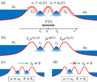
Figure 1: (a) In the reference frame of laboratory, two optical wells are located at $r_{1}$ and $r_{2}$, coupling to the left and right atomic baths, respectively. They are shaking under the driving force $F(t)$. (b) In the shaking frame, tunneling coefficients become time dependent. (c) Atom wave packet occupies both the two optical wells, which leads to stationary current. (d) Coherent trapping occurs with atom wave packet is localized in the first optical well and atomic current is stopped when shaking frequency and shaking strength take particular values, $\omega_{i}$ and $K_{i}$ ($i=1$, $2$, $3$,…).

In this letter, we study coherent control of non-equilibrium atomic transport in a driven atomtronic transistor. Atomtronics study cold atom analogs of electronic circuits and devices Seaman ; Pepino ; Caliga ; Wilsmann , which have been developed experimentally today Wright ; Caliga17 ; Krinner . Firstly, in the driven atomtronic transistor, we prove transition between normal conductor and insulator. The insulator effect is accompanied by coherence of atom occupation in which atom population is coherently trapped in one site of the optical lattice, preserving atoms transit to the other site and dissipated to environment. It is similar to coherent population trapping (CPT) in quantum optics Whitley ; Alzetta ; Arimondo ; Scully . Secondly, for the first time, the coherence induced insulator is analyzed in arbitrary frequency regime, both in $\omega\leq E$ and $\omega>E$. It is thanks to numerical solutions of quantum master equation for the open optical-lattice system. Thirdly, results calculated from the effective Hamiltonian approach and the present numerical approach are compared in the end of this work.

Driven atomtronic transisor$-$The system is schematically illustrated in Fig. 1. The shaken open system is described with the time dependent Hamiltonian $\mathcal{H}(t)=\mathcal{H}_{S}(t)+\mathcal{H}_{E}+\mathcal{H}_{C}$, where the system Hamiltonian which is composed of two shaken optical potential could be written as

$$\mathcal{H}_{S}(t) = \sum_{l=1}^{2}(\varepsilon_{l}+\omega_{l}(t))n_{l}-J(a_{1}^{{\dagger}}a_{2}+a_{2}^{{\dagger}}a_{1}),$$ (1)

where $a_{l}$, $a_{l}^{{\dagger}}$ and $n_{l}=a_{l}^{{\dagger}}a_{l}$ are annihilation, creation and number operators of atoms at lattice site $l$ ($l=1$, $2$), respectively. $\varepsilon_{l}$ denotes bare potential at lattice site $l$. When the potential oscillates periodically, in the reference frame of the potential, cold atoms should feel a oscillating force of inertia $F(t)$. The oscillating inertial force leads to shaken potential that has the form $\omega_{l}(t)=-r_{l}\cdot F(t)$, in which the force get the form $F(t)=F_{\omega}\cos(\omega t)e_{x}$. In the reference frame of a laboratory, positions of the center of optical wells are denoted by $r_{1}=-\frac{d}{2}e_{x}$ and $r_{2}=\frac{d}{2}e_{x}$. The two potentials are coupled with a tunneling strength $J$ of cold atoms. The atomic electrodes are regarded as free atomic gas with the bare energy,

$$\mathcal{H}_{E} = \sum_{\alpha,k}\mu_{\alpha k}n_{\alpha k},$$ (2)

where $a_{\alpha k}$, $a_{\alpha k}^{{\dagger}}$ and $n_{\alpha k}=a_{\alpha k}^{{\dagger}}a_{\alpha k}$ are annihilation, creation and atom number operators in the left ($\alpha=L$) and right ($\alpha=R$) electrodes, respectively. Here, $\mu_{k}$ represents energy of a single atom with momentum $k$. Coupling between the shaken system and atomic electrodes are described by the Hamiltonian,

$$\mathcal{H}_{C} = -\sum_{k}(t_{L}a_{1}^{{\dagger}}a_{Lk}+t_{R}a_{2}^{{\dagger}}a_{Rk}+H.c.),$$ (3)

where $t_{\alpha}$ indicates coupling amplitude between the system and any of the two electrodes.

Quantum master equation$-$Quantum state of the whole configuration is denoted by the total density matrix $\varrho_{tot}$ which consists of the states of the system and its environment. Time evolution of the density matrix $\varrho_{tot}$ satisfies the Liouville-von Neumann equation,

$$\frac{\partial}{\partial t}\varrho_{tot}(t) = -\frac{i}{\hbar}[\mathcal{H}(t),\varrho_{tot}(t)].$$ (4)

Under the transformation of a unitary operator $U(t)=\exp[i\sum_{l=1}^{2}\chi_{l}(t)n_{l}]$, where $\chi_{l}(t)=-\frac{1}{\hbar}\int_{0}^{t}dt^{\prime}\omega_{l}(t^{\prime})$ in which $\omega_{l}(t)$ is given in the Hamiltonian (1), Eq. (4) would be renewed to be

$$\frac{\partial}{\partial t}\rho_{tot}(t) = -\frac{i}{\hbar}[H(t),\rho_{tot}(t)],$$ (5)

where the density matrix is related to $\rho_{tot}(t)=U^{{\dagger}}(t)\varrho_{tot}(t)U(t)$ and the Hamiltonian becomes $H(t)=U^{{\dagger}}(t)\mathcal{H}(t)U(t)-i\hbar U^{{\dagger}}(t)\frac{\partial}{\partial t}U(t)$, which has the detail expression

$$H(t) = \sum_{l=1}^{2}\varepsilon_{l}n_{l}-J(e^{i\phi(t)}a_{1}^{{\dagger}}a_{2}+H.c.)+\sum_{\alpha,k}\mu_{\alpha k}n_{\alpha k}$$ (6)

$$-\sum_{k}(t_{L}(t)a_{1}^{{\dagger}}a_{Lk}+t_{R}(t)a_{2}^{{\dagger}}a_{Rk}+H.c.),$$

where the relative phase is $\phi(t)=\chi_{2}(t)-\chi_{1}(t)$, at the same time, additional phases appear beside the bare tunneling amplitudes as $t_{L}(t)=t_{L}e^{-i\chi_{1}(t)}$ and $t_{R}(t)=t_{R}e^{-i\chi_{2}(t)}$, respectively. From the above definition, one can deduce that $\chi_{2}(t)=-\chi_{1}(t)=\frac{K}{2\hbar\omega}\sin(\omega t)$ and $\phi(t)=\frac{K}{\hbar\omega}\sin(\omega t)$, in which $K$ is the shaking strength $K=F_{\omega}d$. Hamiltonian (6) is important in our work as the starting point of all the following investigations.

Using the gauge-transformed Hamiltonian (7), one can derive the quantum master equation of the system with time-varying coefficients,

$$\frac{\partial}{\partial t}\rho = -i[\sum_{l=1}^{2}\varepsilon_{l}n_{l}-J(e^{i\phi(t)}a_{1}^{{\dagger}}a_{2}+H.c.),\rho]$$ (7)

$$+\mathcal{L}_{L}\rho+\mathcal{L}_{R}\rho,$$

where the system density matrix is $\rho=e^{-\frac{it}{\hbar}H_{0}}\hat{\rho}e^{\frac{it}{\hbar}H_{0}}$. The Lindblad super operators reveals atom leakage between the system and atomic electrodes, they have the typical formulations as

$$\mathcal{L}_{L}\rho = \frac{\Gamma_{L}}{2}(1-f_{L}(\varepsilon_{1}))(2a_{1}\rho a_{1}^{{\dagger}}-\{a_{1}^{{\dagger}}a_{1},\rho\})$$ (8)

$$+\frac{\Gamma_{L}}{2}f_{L}(\varepsilon_{1})(2a_{1}^{{\dagger}}\rho a_{1}-\{a_{1}a_{1}^{{\dagger}},\rho\})$$

and

$$\mathcal{L}_{R}\rho = \frac{\Gamma_{R}}{2}(1-f_{R}(\varepsilon_{2}))(2a_{2}\rho a_{2}^{{\dagger}}-\{a_{2}^{{\dagger}}a_{2},\rho\})$$ (9)

$$+\frac{\Gamma_{R}}{2}f_{R}(\varepsilon_{2})(2a_{2}^{{\dagger}}\rho a_{2}-\{a_{2}a_{2}^{{\dagger}},\rho\}).$$

where the braces here represents anti commutations. The coupling rates read $\Gamma_{L}=2\pi D(\varepsilon_{1})|t_{L}|^{2}$ and $\Gamma_{R}=2\pi D(\varepsilon_{2})|t_{R}|^{2}$. In addition, $f_{L}(\varepsilon_{1})$ and $f_{R}(\varepsilon_{2})$ represent the Fermi-Dirac distribution functions $f_{L}(\varepsilon_{1})=\frac{1}{e^{(\varepsilon_{1}-\mu_{L})/k_{B}T}+1}$ and $f_{R}(\varepsilon_{2})=\frac{1}{e^{(\varepsilon_{2}-\mu_{R})/k_{B}T}+1}$ with Boltzmann constant $k_{B}$ and the temperature of the environment $T$.

Numerical solutions and discussions$-$We solve equation of motion of the system Eq.(7) numerically, since it is a differential equation system whose coefficient is time dependent. Formally, Eq.(7) can be written as $\frac{\partial}{\partial t}\rho=M(t)\rho$ and it has a solution $\rho=e^{N(t)}\rho(0)$, where $N(t)=\int_{0}^{t}M(t^{\prime})dt^{\prime}$ with the evolution matrix $M(t)$ extracted from Eq. (7), $\rho(0)$ represents initial state of the system. By decomposing the evolution matrix one can reach the solutions $\rho=V(t)e^{\Lambda(t)}V^{-1}(t)\rho(0)$, where $V(t)$ and $\Lambda(t)$ are eigenvector and eigenvalue matrices of $N(t)$ at any time, respectively. In this system, single atom occupation is considered in each optical well, therefore, the double well system is characterized by the series of basic states $|00\rangle$, $|01\rangle$, $|10\rangle$ and $|11\rangle$. It is convenient to represent Eq. (7) in the Hilbert space of these basic states.

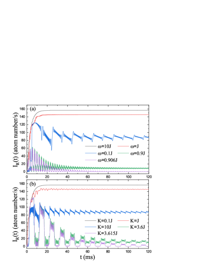
Figure 2: (Color on line) (a) Atomic current as a function of time with different shaking frequencies at $K=5J$. (b) Time dependence of the atomic current with different shaking strengths at $\omega=0.2J$. Parameters: $\theta=0$.

Outcome of the system is current of atomic gas. Atomic current could be derived from the continuity equation $I_{L}-I_{R}=\frac{\partial}{\partial t}Tr_{S}[\rho(t)\sum_{l=1}^{2}a_{l}^{{\dagger}}a_{l}]$, where $I_{L}$ and $I_{R}$ are currents detected in the left side and right side, respectively. $Tr_{S}$ indicates trace over the system states. From this approach, we have the right side current,

$$I_{R} = -\Gamma_{R}f_{R}(\varepsilon_{2})(\rho_{00,00}+\rho_{10,10})$$ (10)

$$+\Gamma_{R}(1-f_{R}(\varepsilon_{2}))(\rho_{01,01}+\rho_{11,11}),$$

which is supposed to be measured in the right electrode. The basic parameters throughout this article are $J=2\pi\times 500$ Hz, $\Gamma_{L}=\Gamma_{R}=0.1J$, $k_{B}T=0.1J$, $\varepsilon_{1}=\varepsilon_{2}=5J$, $\mu_{L}=10J$, $\mu_{R}=0$.

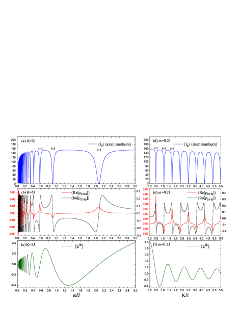
Figure 3: (Color on line) (a)-(c) Spectrum of the averaged current $\langle I_{R}\rangle$, the off-diagonal density matrix element $\langle$Re$[\rho_{0110}]\rangle$ and $\langle$Im$[\rho_{0110}]\rangle$ versus the shaking frequency $\omega$. (d)-(f) Spectrum of the averaged current $\langle I_{R}\rangle$, the off-diagonal density matrix element $\langle$Re$[\rho_{0110}]\rangle$ and $\langle$Im$[\rho_{0110}]\rangle$ as a function of the shaking amplitude $K$. Parameters: $\theta=0$.

Atomic current in the open system as a function of time is shown in Fig. 2. Under the large enough chemical potential bias $\mu_{R}>\varepsilon_{1}$, $\varepsilon_{2}>\mu_{L}$, as we set in the two atomic electrodes (see Fig. 1), stationary current should appear in the system without any external force. However, the system may changed under a shaking of the optical potential. Fig. 2 (a) and (b) show the open system still outcomes stationary current, suffering from shaking with much high frequency $\omega\gg J$ or much small shaking strength $K\ll J$. When the shaking frequency $\omega$ is comparable with the tunneling rate $J$ or even lower, ar the same time, when the shaking strength $K$ is comparable with the tunneling rate $J$ or even larger, current would fluctuate along with time. The current decrease under the shaking is consistent with the change of effective tunneling rate in shaking optical lattices reported previously Creffield6 ; Lignier ; Kierig ; Eckardt ; Zenesini . What we find in our system is that, in the range of low shaking frequency, when we take a particular frequency like $\omega=0.906J$ or a particular shaking strength like $K=3.615J$, system current fluctuates a short time and then tends to disappear as illustrated in Fig. 2.

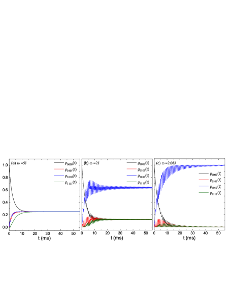
Figure 4: (Color on line) Time evolution of diagonal density matrix elements (probabilities of atom occupation) with different shaking frequencies at $K=5J$. Parameters: $\theta=0$.

To see the system behavior in large parameter range, atomic currents are averaged through real time with the expression

$$\langle I_{R}\rangle=\frac{1}{\tau}\int_{0}^{\tau}I_{R}(t)dt,$$ (11)

as we always do for AC current in electrical engineering. Here, the time range $\tau$ is taken to be $1$s in the numerical treatment throughout this article. The current spectrums in Fig. 3 (a) and (d) show there are many insulation points (the positions of rapid drop of current) under variations of the shaking frequency $\omega$ and the shaking strength $K$. The insulation pints are signed with serial number $i=1$, $2$, $3$, …, just for clear distinction in the figures. They corresponding to the parameter positions $(\omega_{i}$, $K_{i})$, $(\omega_{2}$, $K_{2})$, $(\omega_{3}$, $K_{3})$, …, and so on. Interestingly, insulation points are mapping with change of the off-diagonal density matrix $\rho_{0110}$ one by one, which can be seen comparing Fig. 3 (a) and (b), or (d) and (e). This is the reason we term this phenomenon as coherent insulation. In linear system of differential equations extracted from Eq.(7), the six density matrix elements $\rho_{0000}$, $\rho_{0101}$, $\rho_{1010}$, $\rho_{1111}$, $\rho_{0110}$ and $\rho_{1001}$ connect each other and form a closed space. Therefore, $\rho_{0110}$ (or its complex conjugate $\rho_{1001}$) is the only density matrix element which describes coherence of the system. The average quantities $\langle$Re$[\rho_{0110}]\rangle$ and $\langle$Im$[\rho_{0110}]\rangle$ are achieved in the same way as Eq.(11). Going back to the Hamiltonian, the time dependent phase $\phi(t)$ is at the heart of our time dependent Hamiltonian approach, which describes the shaking dynamics. Indeed, timely averaged phase term $\langle e^{i\phi}\rangle$ is plotted in Fig. 3 (c) and (f). Fluctuation of the phase factor $\langle e^{i\phi}\rangle$ is absolutely match with the behavior of current and off-diagonal density matrix. It means the coherent tunneling term in Eq.(7) is significant for the insulation points.

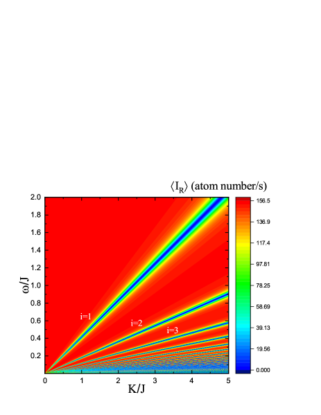
Figure 5: (Color on line) Current spectrum in the space of shaking frequency $\omega$ and shaking strength $K$. Blue lines are the area in which system would behaves as insulation. Parameters: $\theta=0$.

To ascertain what is happening correspondingly in the system, time evolution of diagonal density matrix elements are plotted in Fig. 4, which reflect occupation probabilities of atoms in the two optical wells. For driven frequency $\omega=5J$ in Fig. 4 (a), all probable states are occupied equally. It matches with the stationary current similar to the current line $\omega=10J$ in Fig. 2 (a). For the shaking frequency $\omega=2J$ in Fig. 4 (b), $\rho_{1010}>\rho_{0000}$, $\rho_{0101}$, $\rho_{1111}$, it means atoms are more likely to occupy the first (left) optical well of the system. In this case, current would decrease, its behavior is similar to the lines of $\omega=0.1J$ or $\omega=0.9J$ shown in Fig. 2 (a). Most interestingly, when the frequency is set to be $\omega=2.08$ in Fig. 4 (c), the matrix element $\rho_{1010}$ is increased and close to be $1$. At the same time, the other matrix elements $\rho_{0000}$, $\rho_{0101}$ and $\rho_{1111}$ are decreased to nearly $0$, due to the normalization condition of probabilities in quantum mechanics. In this situation, the current behavior is similar to the line of frequency $\omega=0.906$ in Fig. 2 (a). Current decay at the frequency $\omega=2.08$ is shown in Fig. 3 (a) with the number $i=1$ and current decay at the frequency $\omega=0.906$ is at the position of $i=2$ in Fig. 3 (a). Now it is clear that, insulation in the system is originated from the fact that atoms would be located in one optical well and the other well become empty after a short time evolution. Since this process is also related to coherence of the system, it should be the coherent population trapping. Coherent population trapping is widely studied in quantum optics, in which atom internal states are driven by laser fields Whitley ; Alzetta ; Arimondo ; Scully .

Average current as a function of both shaking frequency and shaking strength are shown in Fig. 5. In the red areas, system outcomes current normally. In contrast, the blue areas are current valleys where the open optical lattice transistor is characterized by the feature of insulation with nearly zero current. Due to the structure of the phase $\phi(t)$ being inverse proportional to shaking frequency $\omega$, the current valleys become very dense when the frequency tends to zero.

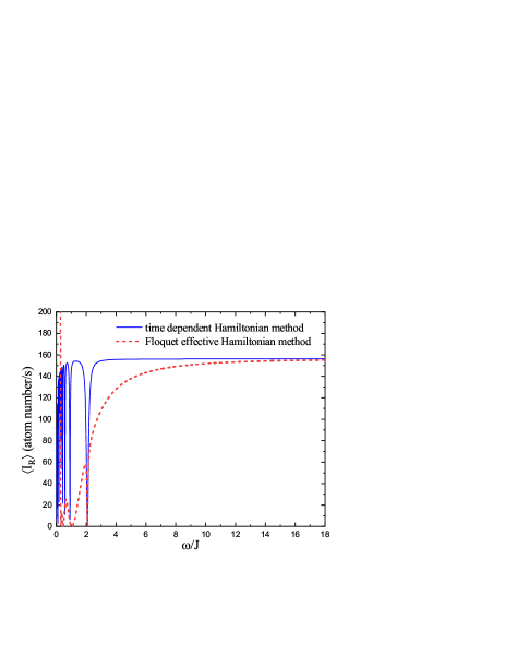
Figure 6: Comparison between the results from time-dependent Hamiltonian approach and Floquet effective Hamiltonian approach. Parameters: $K=5J$, $\theta=0$.

Floquet theory approach$-$ In the end of this work, we would like to compare our time dependent Hamiltonian method with Floquet effective Hamiltonian method. When shaken frequency $\omega$ is much larger than other energy scale, Floquet theory can be used to deal with the time dependent Hamiltonian. According to the Floquet theory, the equality $H_{eff}=\frac{1}{T}\int_{0}^{T}H(t^{\prime})dt^{\prime}$ is satisfied, where $T=\frac{2\pi}{\omega}$. This process gives us an effective Hamiltonian $H_{eff}$,

$$H_{eff} = \sum_{l=1}^{2}\varepsilon_{l}n_{l}-J_{eff}(a_{1}^{{\dagger}}a_{2}+a_{2}^{{\dagger}}a_{1})+\sum_{\alpha,k}\mu_{\alpha k}n_{\alpha k}$$ (12)

$$-\sum_{k}(t_{eff}^{L}a_{1}^{{\dagger}}a_{Lk}+t_{eff}^{R}a_{2}^{{\dagger}}a_{Rk}+H.c.),$$

where $J_{eff}=JJ_{0}(W_{2}-W_{1})$, $t_{eff}^{L}=t_{L}J_{0}(W_{1})$, $t_{eff}^{R}=t_{R}J_{0}(W_{2})$ and $W_{l}=\frac{F_{\omega}}{\hbar\omega}(x_{l}\cos(\alpha)+y_{l}\sin(\alpha))$ with $l=1$, $2$ correspondingly. Here, $J_{0}$ is the zero order Bessel function.

From the effective Hamiltonian (12), we could derive the following mater equation which is similar to the equation of motion (7) except the second term on the right side of the equation,

$$\frac{\partial}{\partial t}\varrho = -i[\sum_{l=1}^{2}\varepsilon_{l}n_{l}-J_{eff}(a_{1}^{{\dagger}}a_{2}+a_{2}^{{\dagger}}a_{1}),\varrho]$$ (13)

$$+\mathcal{L}_{eff}^{L}\varrho+\mathcal{L}_{eff}^{R}\varrho,$$

where $\varrho$ represents density matrix for atomic states evaluated from the effective Hamiltonian (12). The super operators are $\mathcal{L}_{eff}^{L}\varrho=\frac{\Gamma_{eff}^{L}}{2}(1-f_{L}(\varepsilon_{1}))(2a_{1}\varrho a_{1}^{{\dagger}}-\{a_{1}^{{\dagger}}a_{1},\varrho\})+\frac{\Gamma_{eff}^{L}}{2}f_{L}(\varepsilon_{1})(2a_{1}^{{\dagger}}\varrho a_{1}-\{a_{1}a_{1}^{{\dagger}},\varrho\})$ and $\mathcal{L}_{eff}^{R}\varrho=\frac{\Gamma_{eff}^{R}}{2}(1-f_{R}(\varepsilon_{2}))(2a_{2}\varrho a_{2}^{{\dagger}}-\{a_{2}^{{\dagger}}a_{2},\varrho\})+\frac{\Gamma_{eff}^{R}}{2}f_{R}(\varepsilon_{2})(2a_{2}^{{\dagger}}\varrho a_{2}-\{a_{2}a_{2}^{{\dagger}},\varrho\})$. Here, we have $\Gamma_{eff}^{L}=\Gamma_{L}J_{0}^{2}(W_{1})$ and $\Gamma_{eff}^{R}=\Gamma_{R}J_{0}^{2}(W_{2})$.

The Floquet effective Hamiltonian approach requires shaking (driving) frequency is large enough compared with other energy scales. Indeed, Fig. 6 shows that the Floquet effective Hamiltonian approach consists with time-dependent Hamiltonian approach in the high frequency regime, $\omega\gg J$. In the low frequency region, difference between the two methods become very large. Interestingly, in the low frequency region, the Floquet effective Hamiltonian approach weakly reflect a few insulation points. However, in the limit of shaking frequency tends to zero, the Floquet effective Hamiltonian approach gives rise to infinitely large current value. In contrast, the time-dependent Hamiltonian approach offers frequently changing current. The time-dependent Hamiltonian approach developed here should be more general protocol to deal with dynamics of the shaken quantum system.

Conclusions$-$Using the time-dependent Hamiltonian numerical method, we studied shaken optical lattice transistor within low shaking frequency regime. Abrupt drop of atomic current was predicted under external chemical potential bias and optical potential shaking. We find the current drop is originated from coherence of the atom states in optical wells. Time dependent phase term in the Hamiltonian plays important role for this coherent process. The present work offers supplemental research of the shaken optical lattice in low shaking frequency band.

References

- (1) F. Grossmann, T. Dittrich, P. Jung, and P. Hänggi, Phys. Rev. Lett. 67, 516 (1991).
- (2) M. Grifoni, P. Hänggi, Physics Reports 304, 229 (1998).
- (3) E. Kierig, U. Schnorrberger, A. Schietinger, J. Tomkovic, and M. K. Oberthaler, Phys. Rev. Lett. 100, 190405 (2008).
- (4) H. Lignier, C. Sias, D. Ciampini, Y. Singh, A. Zenesini, O. Morsch, and E. Arimondo, Phys. Rev. Lett. 99, 220403 (2007).
- (5) André Eckardt, Christoph Weiss, and Martin Holthaus, Phys. Rev. Lett. 95, 260404 (2005).
- (6) C. E. Creffield and T. S. Monteiro, Phys. Rev. Lett. 96, 210403 (2006).
- (7) Alessandro Zenesini, Hans Lignier, Donatella Ciampini, Oliver Morsch, and Ennio Arimondo, Phys. Rev. Lett. 102, 100403 (2009).
- (8) Anders S. Sørensen, Eugene Demler, and Mikhail D. Lukin, Phys. Rev. Lett. 94, 086803 (2005).
- (9) Shiwan Miao, Zhongchi Zhang, Yajuan Zhao, Zihan Zhao, Huaichuan Wang, and Jiazhong Hu, Phys. Rev. B 106, 054310 (2022).
- (10) Takuya Kitagawa, Erez Berg, Mark Rudner, and Eugene Demler, Phys. Rev. B 82, 235114 (2010).
- (11) Mark S. Rudner, Netanel H. Lindner, Erez Berg, and Michael Levin, Phys. Rev. A 3, 031005 (2013).
- (12) Wei Zheng and Hui Zhai, Phys. Rev. A 89, 061603(R) (2014).
- (13) Karen Wintersperger, Christoph Braun, F. Nur Ünal, André Eckardt, Marco Di Liberto, Nathan Goldman, Immanuel Bloch and Monika Aidelsburger, Nat. Phys. 16, 1058 (2020).
- (14) Shujie Cheng, Honghao Yin, Zhanpeng Lu, Chaocheng He, Pei Wang, and Gao Xianlong, Phys. Rev. A 101, 043620 (2020).
- (15) Jin-Yi Zhang, Chang-Rui Yi, Long Zhang, Rui-Heng Jiao, Kai-Ye Shi, Huan Yuan, Wei Zhang, Xiong-Jun Liu, Shuai Chen, and Jian-Wei Pan, Phys. Rev. Lett. 130, 04320 (2023).
- (16) Feng Mei, Jia-Bin You, Dan-Wei Zhang, X. C. Yang, R. Fazio, Shi-Liang Zhu, and L. C. Kwe, Phys. Rev. A 90, 063638 (2014).
- (17) Jin Hyoun Kang and Yong-il Shin, Phys. Rev. A 102, 063315 (2020).
- (18) Yanlin Feng, Jingtao Fan, Xiaofan Zhou, Gang Chen, and Suotang Ji, Phys. Rev. A 99, 043630 (2019).
- (19) Bo Song, Shovan Dutta, Shaurya Bhave, Jr-Chiun Yu, Edward Carter, Nigel Cooper, and Ulrich Schneider, Nat. Phys. 18, 259 (2022).
- (20) J. Struck, C. Ölschläger, M. Weinberg, P. Hauke, J. Simonet, A. Eckardt, M. Lewenstein, K. Sengstock, and P. Windpassinger, Phys. Rev. Lett. 108, 225304 (2012).
- (21) Philipp Hauke, Olivier Tieleman, Alessio Celi, Christoph Ölschläger, Juliette Simonet, Julian Struck, Malte Weinberg, Patrick Windpassinger, Klaus Sengstock, Maciej Lewenstein, and André Eckardt, Phys. Rev. Lett. 109, 145301 (2012).
- (22) C. E. Creffield, G. Pieplow, F. Sols and N. Goldman, New J. Phys. 18, 093013 (2016).
- (23) Hannah M. Price, Tomoki Ozawa, and Nathan Goldman, Phys. Rev. A 95, 023607 (2017).
- (24) P. Blanco-Mas and C. E. Creffield, Phys. Rev. A 107, 043310 (2023).
- (25) Kaiyue Wang, Feng Xiong, Yun Long, Yun Ma, and Colin V. Parker, Phys. Rev. A 108, L051302 (2023).
- (26) M. Matti Maricq, Phys. Rev. B 25, 6622 (1982).
- (27) T. P. Grozdanov and M. J. Raković, Phys. Rev. A 38, 1739 (1988).
- (28) N. Goldman, J. Dalibard, Phys. Rev. X 4, 0310275 (2014).
- (29) A. Eckardt, Rev. Mod. Phys. 89, 011004 (2017).
- (30) Gaoyong Sun and André Eckardt, Phys. Rev. Research 2, 013241 (2020).
- (31) Michael Vogl, Martin Rodriguez-Vega, and Gregory A. Fiete, Phys. Rev. B 101, 024303 (2020).
- (32) Michael Vogl, Martin Rodriguez-Vega, and Gregory A. Fiete, Phys. Rev. B 101, 235411 (2020).
- (33) B. T. Seaman, M. Krämer, D. Z. Anderson, and M. J. Holland, Entropy 75, 023615 (2007).
- (34) R. A. Pepino, J. Cooper, D. Z. Anderson, and M. J. Holland, Phys. Rev. Lett. 103, 140405 (2009).
- (35) Seth C. Caliga, Cameron J. E. Straatsma, Alex A. Zozulya and Dana Z. Anderson, New J. Phys. 18, 015012 (2016).
- (36) Karin Wittmann Wilsmann, Leandro H. Ymai, Arlei Prestes Tonel, Jon Links, and Angela Foerster, Commun. Phy. 1, 91 (2018).
- (37) K. C. Wright, R. B. Blakestad, C. J. Lobb, W. D. Phillips, and G. K. Campbell, Phys. Rev. Lett. 110, 025302 (2013).
- (38) Seth C. Caliga, Cameron J. E. Straatsma and Dana Z. Anderson, New J. Phys. 19, 013036 (2017).
- (39) Sebastian Krinner, Tilman Esslinger and Jean-Philippe Brantut, J. Phys.: Condens. Matter 29, 343003 (2017).
- (40) R. M. Whitley and C. R. Stroud, Phys. Rev. A 14, 1498 (1976).
- (41) G. Alzetta, A. Gozzini, L. Moi, and G. Orriols, Nuovo Cimento Soc. Ital. Fis., B 36, 5 (1976).
- (42) E. Arimondo, Prog. Opt. 35, 257 (1996).
- (43) M. O. Scully and M. S. Zubairy, Quantum Optics, Cambridge: Cambridge University Press, (1997).